Limiting spectral distribution of renormalized separable sample covariance matrices when $p/n\to 0$

Abstract

We are concerned with the behavior of the eigenvalues of renormalized sample covariance matrices of the form

$$C_{n}=\sqrt{\frac{n}{p}}\left(\frac{1}{n}A_{p}^{1/2}X_{n}B_{n}X_{n}^{*}A_{p}^{1/2}-\frac{1}{n}\mbox{tr}(B_{n})A_{p}\right)$$

as $p,n\to\infty$ and $p/n\to 0$, where $X_{n}$ is a $p\times n$ matrix with i.i.d. real or complex valued entries $X_{ij}$ satisfying $E(X_{ij})=0$, $E|X_{ij}|^{2}=1$ and having finite fourth moment. $A_{p}^{1/2}$ is a square-root of the nonnegative definite Hermitian matrix $A_{p}$, and $B_{n}$ is an $n\times n$ nonnegative definite Hermitian matrix. We show that the empirical spectral distribution (ESD) of $C_{n}$ converges a.s. to a nonrandom limiting distribution under the assumption that the ESD of $A_{p}$ converges to a distribution $F^{A}$ that is not degenerate at zero, and that the first and second spectral moments of $B_{n}$ converge. The probability density function of the LSD of $C_{n}$ is derived and it is shown that it depends on the LSD of $A_{p}$ and the limiting value of $n^{-1}\mbox{tr}(B_{n}^{2})$. We propose a computational algorithm for evaluating this limiting density when the LSD of $A_{p}$ is a mixture of point masses. In addition, when the entries of $X_{n}$ are sub-Gaussian, we derive the limiting empirical distribution of $\{\sqrt{n/p}(\lambda_{j}(S_{n})-n^{-1}\mbox{tr}(B_{n})\lambda_{j}(A_{p}))\}_{j=1}^{p}$ where $S_{n}:=n^{-1}A_{p}^{1/2}X_{n}B_{n}X_{n}^{*}A_{p}^{1/2}$ is the sample covariance matrix and $\lambda_{j}$ denotes the $j$-th largest eigenvalue, when $F^{A}$ is a finite mixture of point masses. These results are utilized to propose a test for the covariance structure of the data where the null hypothesis is that the joint covariance matrix is of the form $A_{p}\otimes B_{n}$ for $\otimes$ denoting the Kronecker product, as well as $A_{p}$ and the first two spectral moments of $B_{n}$ are specified. The performance of this test is illustrated through a simulation study.

Keywords. Separable covariance; limiting spectral distribution; Stieltjes transform; McDiarmid’s inequality; Lindeberg principle, Wielandt’s inequality.

AMS subject classification: 60B20, 62E20, 60F05, 60F15, 62H99

1 Introduction

In this paper, we obtain the limiting spectral distribution (LSD) and a system of equations describing the corresponding Stieltjes transforms of renormalized sample covariance matrices of the form

$$C_{n}=\sqrt{\frac{n}{p}}\left(\frac{1}{n}A_{p}^{1/2}X_{n}B_{n}X_{n}^{*}A_{p}^{1/2}-\frac{1}{n}\mbox{tr}(B_{n})A_{p}\right)$$ (1.1)

when $p,n\to\infty$ and $p/n\to 0$, where $X_{n}$ has i.i.d. real or complex entries with zero mean, unit variance and uniformly bounded fourth moment. Throughout this paper, for any matrix $M$, we use $M^{*}$ to denote the complex conjugate transpose of $M$ if $M$ is complex-valued and transpose of $M$ if $M$ is real-valued. When $p/n\to c\in(0,+\infty)$ as $n\to\infty$, the spectral properties of the separable sample covariance matrices, $S_{n}:=n^{-1}A_{p}^{1/2}X_{n}B_{n}X_{n}^{*}A_{p}^{1/2}$ have been widely investigated under different assumptions on entries (e.g., Zhang [31], Paul and Silverstein [23], EL Karoui [9]). The name “separable” refers to the fact that the covariance matrix of the vectorized data matrix $Y_{n}=A_{p}^{1/2}X_{n}B_{n}^{1/2}$ has the separable covariance $A_{p}\otimes B_{n}$, where $\otimes$ denotes the Kronecker product between matrices. Under those circumstances, it is known that the spectral norm of $S_{n}-\mathbb{E}S_{n}$ does not converge to zero. However, if $p/n\to 0$, $\parallel S_{n}-\mathbb{E}S_{n}\parallel\stackrel{{\scriptstyle a.s.}}{{\longrightarrow}}0$. When $A_{p}=I_{p},B_{n}=I_{n}$ and $p,n\to\infty$ such that $p/n\to 0$, the behavior of empirical spectral distribution (ESD) of $\sqrt{n/p}\left(S_{n}-\mathbb{E}S_{n}\right)=\sqrt{n/p}(n^{-1}X_{n}X_{n}^{*}-I_{p})$ is similar to that of a $p\times p$ Wigner matrix $W_{p}$, which has been verified by Bai and Yin [3]. Moreover, when $S_{n}=n^{-1}A_{p}^{1/2}X_{n}X_{n}^{*}A_{p}^{1/2}$, for i.i.d. real entries and under a finite fourth moment condition, Pan and Gao [20] and Bao [5] derived the LSD of $\sqrt{n/p}(n^{-1}A_{p}^{1/2}X_{n}X_{n}^{*}A_{p}^{1/2}-A_{p})$, which coincides with that of a generalized Wigner matrix $p^{-1/2}A_{p}^{1/2}W_{p}A_{p}^{1/2}$ studied by Bai and Zhang [4]. Our work here extends the former result to a more general setting, namely, when $B_{n}$ is an arbitrary $n\times n$ positive semi-definite matrix whose first two spectral moments converge to finite positive values as $n\to\infty$, and the entries of $X_{n}$ are either real or complex. The strategy of the proof of this result is divided into three parts. We first assume that the entries of $X_{n}$ are i.i.d. Gaussian and use a construction analogous to that in Pan and Gao [20] to obtain the form of the approximate deterministic equations describing the expected Stieltjes transforms, then use a result on concentration of smooth functions of independent random elements to show that the Stieltjes transform concentrates around its mean in the general setting (without the restriction of Gaussianity), and finally utilize the Lindeberg principle to show that the expected Stieltjes transforms in the Gaussian and in the general case are asymptotically the same. In the process, we also prove the existence and uniqueness of the system of equations describing the Stieltjes transform for an arbitrary $F^{A}$, non-degenerate at zero. Further, we state a result characterizing the LSD, including the existence and shape of its density function, by following the approach in Bai and Zhang [4]. We also study the question of fluctuation of the eigenvalues of the sample covariance matrix $S_{n}:=n^{-1}A_{p}^{1/2}X_{n}B_{n}X_{n}^{*}A_{p}^{1/2}$ itself when the ESD of $A_{p},$ say $F^{A_{p}}$ and its limit $F^{A}$ are finite mixtures of point masses. Specifically, we show that the empirical distribution of $\{\sqrt{n/p}(\lambda_{j}(S_{n})-n^{-1}\mbox{tr}(B_{n})\lambda_{j}(A_{p}))\}_{j=1}^{p}$, where $\lambda_{j}$ denotes the $j$-th largest eigenvalue, converges a.s. to a mixture of rescaled semi-circle laws with mixture weights being the same as the weights corresponding to the point masses of $F^{A}$ and the scaling factor depending on the limiting value of $n^{-1}\mbox{tr}(B_{n}^{2})$ and the atoms of $F^{A}$.

It should be noted that the data model of the form $Y_{n}=A_{p}^{1/2}X_{n}B_{n}^{1/2}$, where $X_{n}$ has i.i.d. entries with zero mean and unit variance, relates very closely to the separable covariance model widely used in spatio-temporal data modeling, especially for modeling environmental data (e.g., Kyriakidis and Journel [11], Mitchell and Gumpertz [13], Fuentes [10], Li et al. [17]). The separable covariance model refers to the fact that for any $p$ sampling locations in space, and any $n$ observation times, the covariance of the corresponding data matrix can be expressed in the form $\Sigma_{n,p}=A_{p}\otimes B_{n}$. In that context, the rows of $Y_{n}$ correspond to spatial locations while the columns represent the observation times. If furthermore, the process is Gaussian, which is often assumed in the literature, then the data matrix $Y_{n}$ is exactly of the form $A_{p}^{1/2}X_{n}B_{n}^{1/2}$ where $X_{ij}$’s are i.i.d. $N(0,1)$. Assuming a separable covariance structure, that the process is stationary in space, the sampling locations cover the entire spatial region under consideration fairly evenly, and the temporal variation has only short term dependence (not necessarily stationary), the covariance of the observed data can be expressed in the form $A_{p}\otimes B_{n}$ where $A_{p}$ and $B_{n}$ satisfy conditions 3, 4 and 5 of our main result in this paper (Theorem 2.1). Moreover, if the sampling locations are on a spatial grid, then the matrix of eigenvectors of $A_{p}$ is approximately the Fourier rotation matrix on $\mathbb{R}^{p}$ and the eigenvalues are approximately the Fourier transform of the spatial autocovariance kernel evaluated at certain discrete frequencies related to the grid spacings.

There is a body of literature on the statistical inference for a separable covariance model, in particular about the tests for separability of the joint covariance of the data. Notable examples include Dutilleul [7], Lu and Zimmerman [18], Mitchell et al. ([14], [15]), Fuentes [10], Roy and Khatree [24], Simpson [28] and Li et al. [17]. These tests typically assume joint Gaussianity of the data and often the derivation of the test statistic requires additional structural assumptions, e.g., stationarity of the spatial and temporal processes (Fuentes [10]). In addition, the estimation techniques often involve matrix inversions (Dutilleul [7], Mitchell et al. [15]) which become challenging if the dimensionality (either $p$ or $n$) is large. We study the problem of tests involving the separable covariance structure under the framework $p,n\to\infty$ and $p/n\to 0$. Under this setting, $\parallel n^{-1}Y_{n}Y_{n}^{*}-n^{-1}\mbox{tr}(B_{n})A_{p}\parallel\stackrel{{\scriptstyle a.s.}}{{\longrightarrow}}0$ and hence we can infer about the spectral properties of $A_{p}$ from that of the sample covariance matrix $n^{-1}Y_{n}Y_{n}^{*}$. In particular, we propose to use the results derived here to construct test statistic for testing whether the space-time data follows a specific separable covariance model, where the null hypothesis is in terms of specification of $A_{p}$ and the first two spectral moments of $B_{n}$. Let $A_{0}$, $\mbox{tr}(B_{0})$ and $\mbox{tr}(B_{0}^{2})$ be the specified values of $A_{p}$, $\mbox{tr}(B_{n})$ and $\mbox{tr}(B_{n}^{2})$ under the null hypothesis, Then this statistic measures the difference of the ESD of the matrix $\sqrt{n/p}(n^{-1}Y_{n}Y_{n}^{*}-n^{-1}\mbox{tr}(B_{0})A_{0})$, from the LSD of $C_{n}$ described in (1.1), where the matrix $X_{n}$ is assumed to have i.i.d. entries with zero mean and unit variance, $A_{p}=A_{0}$, $\mbox{tr}(B_{n})=\mbox{tr}(B_{0})$ and $\mbox{tr}(B_{n}^{2})=\mbox{tr}(B_{0}^{2})$. We also propose a Monte-Carlo method for determination of the cut-off values of the test for any given level of significance and analyze the behavior of the test through simulation. We also carry out a simulation study with different combinations of $(p,n)$ to empirically assess the rate of convergence of the ESD under to the LSD as measured by the $L^{2}$ distance between these distributions.

2 Main results

Under the framework presented in Section 1, our main result in this paper is about the existence and uniqueness of the LSD of $C_{n}$ defined through (1.1). The result will be described in terms of the Stieltjes transform of the matrices. The Stieltjes transform of the empirical spectral distribution $F^{C_{n}}$ is defined as

$$s_{n}(z)=\int\frac{1}{x-z}dF^{C_{n}}(x)$$

for any $z\in\mathbb{C}^{+}:=\{u+iv:u\in\mathbb{R},v>0\}$. It will be shown that the ESD of $C_{n}$ will converge almost surely to a distribution $F$ whose Stieltjes transform is determined by a system of equations.

Theorem 2.1.

Suppose that

1. for every $p$ and $n$, $\{X_{i,j}:1\leq i\leq p,1\leq j\leq n\}$ is an array of i.i.d real or complex valued random variables with $\mathbb{E}(X_{11})=0$, $\mathbb{E}|X_{11}|^{2}=1$ and $\mathbb{E}|X_{11}|^{4}<\infty$;

2. $p=p(n)\to\infty$ with $p(n)/n\to 0$ as $n\to\infty$;

3. $A_{p}$ is a $p\times p$ nonnegative definite Hermitian matrix and $B_{n}$ is a $n\times n$ nonnegative hermitian matrix;

4. the ESD $F^{A_{p}}\Longrightarrow F^{A}$ as $p\to\infty$ where $F^{A}$ is a nonrandom distribution function on $\mathbb{R}_{+}$ that is not degenerate at zero;

5. $\parallel B_{n}\parallel$ is bounded above, and $n^{-1}\mbox{tr}(B_{n}^{k})$ for $k=1,2$ converge to finite positive constants as $n\to\infty$.

Then $F^{C_{n}}$ almost surely converges weakly to a nonrandom distribution $F$ as $n\to\infty$, whose Stieltjes transform $s(z)$ is determined by the following system of equations:

$$\begin{cases}s(z)=-\int\frac{dF^{A}(a)}{z+\bar{b}_{2}a\beta(z)}\\ \beta(z)=-\int\frac{adF^{A}(a)}{z+\bar{b}_{2}a\beta(z)}\end{cases}$$ (2.1)

for any $z\in\mathbb{C}^{+}$, where $\bar{b}_{2}=\displaystyle\lim_{n\to\infty}n^{-1}tr(B_{n}^{2})$.

Remark 2.2.

In (2.1), the constant $\bar{b}_{2}$ determines the scale of the support of the LSD $F$. Specifically, the LSD $F$ is related to the LSD $F_{A,I}$ corresponding to the case $B_{n}=I_{n}$ (studied by Pan and Gao [20] and Bao [5]), by $F(x)=F_{A,I}(\bar{b}_{2}^{-1/2}x)$ for all $x\in\mathbb{R}$. Note also that, $F_{A,I}$ coincides with the LSD of the generalized Wigner matrix $p^{-1/2}A_{p}^{1/2}W_{p}A_{p}^{1/2}$ analyzed by Bai and Zhang [4].

Remark 2.3.

If $A_{p}=I_{p}$, the two equations (2.1) reduce to only one, namely, $s(z)(z+\bar{b}_{2}s(z))=-1$, which is the equation for a rescaled semi-circle law $F_{sc}(\cdot;\sqrt{\bar{b}_{2}})$ with scaling factor $\sqrt{\bar{b}_{2}}$, where, for any $\sigma>0$,

$$F_{sc}(x;\sigma):=F_{sc}(\sigma^{-1}x),\qquad\mbox{for all}~{}~{}x\in\mathbb{R},$$ (2.2)

where $F_{sc}$ denotes the semi-circle law. Notice that, in this case due to the rotational invariance, the statement of the Theorem 2.1 reduces to the statement that the empirical distribution of $\{\sqrt{n/p}(\lambda_{j}(S_{n})-n^{-1}\mbox{tr}(B_{n}))\}_{j=1}^{p}$, converges a.s. to the rescaled semi-circle law with scaling factor $\bar{b}_{2}$. We present an interesting generalization of this result in Section 2.2.

Remark 2.4.

In the statement of Theorem 2.1, the matrix $A_{p}^{1/2}$ needs not be the Hermitian square root of $A_{p}$. As long as $(A_{p}^{1/2})(A_{p}^{1/2})^{*}=A_{p}$, the result will continue to hold. In particular, $A_{p}^{1/2}$ can be of the form $A_{p}^{1/2}=U\Lambda^{1/2}V^{*}$, where $A_{p}=U\Lambda U^{*}$ is the spectral decomposition of $A_{p}$, so that $\Lambda$ is a diagonal matrix and $V^{*}V=U^{*}U=I_{p}$. Moreover, from this it also follows that if $\widetilde{V}$ is a $p\times q$ matrix with $q\leq p$ such that $\widetilde{V}^{*}\widetilde{V}=I_{q}$ where $q\to\infty$ such that $q/p\to\omega\in(0,1]$ and $\widetilde{Y}_{n}=\widetilde{V}^{*}X_{n}B_{n}^{1/2}$ then the ESD of $\sqrt{n/q}(n^{-1}\widetilde{Y}_{n}\widetilde{Y}_{n}^{*}-n^{-1}\mbox{tr}(B_{n})I_{q})$ converges a.s. to the distribution $F_{sc}(\cdot;\sqrt{\bar{b}_{2}})$ introduced in Remark 2.3.

Remark 2.5.

Proof of Theorem 2.1 can be divided into the following parts:

1. The spectrum of $A_{p}$ is truncated at a sufficiently large $a_{0}$. This is done in Section 3.1, following an approach in Bai and Yin [3]. It is shown that the ESD of the $C_{n}$ and the matrix corresponding to the truncated $A_{p}$ are almost surely equivalent.

2. For each $z\in\mathbb{C}^{+}$, and for $C_{n}$ corresponding to matrices with i.i.d. standard Gaussian entries, $\mathbb{E}(s_{n}(z))\to s(z)$ satisfying (2.1), which is shown in Section 3.2.

3. For each $z\in\mathbb{C}^{+}$, $s_{n}(z)-\mathbb{E}(s_{n}(z))$ converges almost surely to zero. This is derived in Section 3.3 through the use of McDiarmid’s inequality (McDiarmid [12]).

4. Existence and uniqueness of the solution of the system of equations (2.1) defining the limiting Stieltjes transform $s(z)$ is established in 3.4.

5. The entries of $X_{n}$ are truncated at $n^{1/4}\epsilon_{p}$ and centered, where $\epsilon_{p}\to 0$, $p^{1/4}\epsilon_{p}\to\infty$ which does not alter the LSD. The result is established in the general setting by establishing the asymptotic negligibility of the difference of $\mathbb{E}(s_{n}(z))$ corresponding to independent copies of $X_{n}$ with such truncated entries in Section 3.5.

2.1 Analysis of LSD

The following result characterizes the behavior of the LSD $F$ in Theorem 2.1.

Proposition 2.6.

Suppose that $F^{A}(a)\neq I_{[0,\infty)}(a)$ and let $F$ be the LSD of $F^{C_{n}}$ as in Theorem 2.1. Then, $F(\{0\})=F^{A}(\{0\})$, and for any real $x\neq 0$,

$$s(x)=\lim_{z\in\mathbb{C}^{+}\to x}s(z),\quad\beta(x)=\lim_{z\in\mathbb{C}^{+}\to x}\beta(z)$$

exist such that

$$s(x)=-\int\frac{dF^{A}(a)}{x+\bar{b}_{2}a\beta(x)},$$

where $\beta(x)$ uniquely solves

$$\beta(x)=-\int\frac{adF^{A}(a)}{x+\bar{b}_{2}a\beta(x)}$$ (2.3)

while satisfying $\Im\beta(x)\geq 0$, $x\Re\beta(x)<0$ and $\omega(x)\leq 1$, where

$$\omega(x):=\int\frac{\bar{b}_{2}a^{2}}{|x+\bar{b}_{2}a\beta(x)|^{2}}dF^{A}(a).$$ (2.4)

Moreover, we have

1. $s(x)$ and $\beta(x)$ are continuous on the real line except only at the origin.

2. $F(x)$ is symmetric and continuously differentiable on the real line except at the origin and its derivative is given by

   $$f(x)=-\frac{2\Re\beta(x)\Im\beta(x)}{\pi x}.$$ (2.5)

3. The support of $F$, say $\mathcal{S}$ is determined as follows: for any $x\neq 0$, $x\in\mathcal{S}^{c}$ (complement of $\mathcal{S}$) if and only if there exists some $\delta>0$ such that for all $y\in(x-\delta,x+\delta)$, $\omega(y)<1$.

The proof of this proposition follows along the line of the proof Theorem 1.2 of Bai and Zhang [4] with an additional scale factor $\bar{b}_{2}:=\displaystyle\lim_{n\to\infty}n^{-1}\mbox{tr}(B_{n}^{2})$. The following lemma, which is a consequence of property (3) of Proposition 2.6, provides a way of determining the support of the density function.

Lemma 2.7.

The support of $f(x)$ is the set of $x\in\mathbb{R}$ satisfying $x\Re\beta(x)<0$ and $\omega(x)=1$ (equivalently, $\Im\beta(x)>0$).

A more direct verification of Lemma 2.7 is given in Section 3.4.

2.2 Fluctuation of eigenvalues of $S_{n}$

In certain applications, not only the eigenvalues of $C_{n}$ but difference of the eigenvalues of $S_{n}$ from those of $\mathbb{E}(S_{n})$ may be of interest. Since $\parallel S_{n}-\mathbb{E}(S_{n})\parallel\to 0$, a.s., under the framework $p/n\to 0$, it is expected that the eigenvalues of $S_{n}$ will fluctuate around the “corresponding” eigenvalues of $\mathbb{E}(S_{n})=n^{-1}\mbox{tr}(B_{n})A_{p}$. To make this notion more precise, we consider the setting where there are finitely many distinct eigenvalues of $A_{p}$. Then for large enough $n$, the eigenvalues of $S_{n}$ will tend to cluster around these distinct eigenvalues of $n^{-1}\mbox{tr}(B_{n})A_{p}$. Moreover, if both $\parallel A_{p}\parallel$ and $\parallel B_{n}\parallel$ are bounded, the proportion of eigenvalues falling in each cluster will coincide with the proportion of the corresponding eigenvalue of $A_{p}$ in the ESD of $A_{p}$. This can be seen as an instance of the spectrum separation phenomenon studied by Bai and Silverstein [2] for sample covariance matrices in the setting $p/n\to c\in(0,\infty)$. Our goal in this subsection is to establish that, if $\parallel B_{n}\parallel$ is bounded, and if the probability distribution of the entries of $X_{n}$ has sufficiently fast decay in the tails (specifically, “sub-Gaussian tails”), then the fluctuations of the eigenvalues of $S_{n}$ around the eigenvalues of $n^{-1}\mbox{tr}(B_{n})A_{p}$ can be fully characterized, provided $A_{p}$ has finitely many distinct eigenvalues, the proportion of each of which converges to a nonzero fraction.

To state the result, we first define a sub-Gaussian random vector (cf. Vershynin [30]). A real-valued random vector $\mathbf{y}=(y_{1},\ldots,y_{n})^{T}$ is said to be sub-Gaussian with scale parameter $\sigma\geq 0$, if for all $\gamma\in\mathbb{R}^{n}$,

$$\mathbb{E}[\exp(\gamma^{T}\mathbf{y})]\leq\exp(\parallel\gamma\parallel^{2}\sigma^{2}/2).$$ (2.6)

Clearly, if $\mathbf{y}$ has independent coordinates each of which is sub-Gaussian with scale parameter $\sigma$, then $\mathbf{y}$ is sub-Gaussian. Moreover, it is easy to see that if $\mathbf{y}$ is sub-Gaussian with scale parameter $\sigma$, then for any $m\times n$ matrix $D$, the vector $D\mathbf{y}$ is also sub-Gaussian, with scale parameter $\parallel D\parallel\sigma$. A complex-valued random vector is sub-Gaussian if and only if both real and imaginary parts of the vector are sub-Gaussian.

Theorem 2.8.

Let $B_{n}$ be a $n\times n$ positive semi-definite matrix such that $\parallel B_{n}\parallel$ is bounded above, $n^{-1}\mbox{tr}(B_{n})\to\bar{b}$ and $n^{-1}\mbox{tr}(B_{n}^{2})\to\bar{b}_{2}$ as $n\to\infty$. Let $A_{p}$ be a $p\times p$ positive semidefinite matrix with $m$ distinct eigenvalues $\alpha_{1}>\ldots>\alpha_{m}\geq 0$ such that $\alpha_{1}$ is bounded above and $m$ is fixed, and if $p_{j}$ denotes the multiplicity of $\lambda_{j}$, then $p_{j}/p\to c_{j}>0$ for all $j$, as $p\to\infty$. Let $Y_{n}=A_{p}^{1/2}X_{n}B_{n}^{1/2}$ where $X_{n}$ is a $p\times n$ matrix with i.i.d. real or complex sub-Gaussian entries $X_{ij}$ satisfying $\mathbb{E}(X_{11})=0$ and $\mathbb{E}|X_{11}|^{2}=1$. In the complex case, we also suppose that the real and imaginary parts of $X_{ij}$ are independent with variance $1/2$ each. Let $S_{n}:=n^{-1}Y_{n}Y_{n}^{*}$, and let $\lambda_{j}(D)$ denote the $j$-th largest eigenvalue of a Hermitian matrix $D$. Then, as $p,n\to\infty$ such that $p/n\to 0$, the empirical distribution of $\{\sqrt{n/p}(\lambda_{j}(S_{n})-n^{-1}\mbox{tr}(B_{n})\lambda_{j}(A_{p}))\}_{j=1}^{p}$ converges a.s. to a nonrandom probability distribution $F$ on $\mathbb{R}$ which can be expressed as

$$F(x)=\sum_{j=1}^{m}c_{j}F_{sc}(x;\sqrt{\bar{b}_{2}c_{j}}\alpha_{j}),~{}~{}~{}\mbox{for}~{}x\in\mathbb{R},$$

where $F_{sc}(\cdot;\sigma)$, for any $\sigma>0$, is defined in (2.2).

Remark 2.9.

The assumption of sub-Gaussianity of the entries in Theorem 2.8 is not necessary if $p=o(n^{1/3})$. In that case, if we only assume the finiteness of $\mathbb{E}|X_{11}|^{4}$, it can be shown that the empirical distribution of $\{\sqrt{n/p}(\lambda_{j}(S_{n})-n^{-1}\mbox{tr}(B_{n})\lambda_{j}(A_{p}))\}_{j=1}^{p}$ converges in probability to the same limit law. This is because, as is seen from the proof given in Section 4, without loss of generality assuming $m=2$, the conclusion follows upon showing that $\sqrt{n/p}\parallel S_{12}\parallel^{2}=o_{P}(1)$, which can be majorized by $\sqrt{n/p}\parallel S_{12}\parallel_{F}^{2}$, where $\parallel\cdot\parallel_{F}$ denotes the Frobenius norm. The latter is $O_{P}(\sqrt{n/p}(p^{2}/n))=o_{P}(1)$ under the stated conditions. A stronger conclusion (in the form of a.s. convergence) can be made with appropriately higher moment conditions.

2.3 Application to hypothesis testing

The results in the previous subsections allow us to develop a test for the hypothesis that data matrix $Y_{n}$ has a specific separable covariance structure. Suppose that the vectorized $Y_{n}$ has joint covariance $\Sigma_{n}$. Then our null hypothesis is that

$$H_{0}:\Sigma_{n}=A_{p}\otimes B_{n}~{}\mbox{with}~{}A_{p}=A_{0},n^{-1}\mbox{tr}(B_{n})=\bar{b}^{0},n^{-1}\mbox{tr}(B_{n}^{2})=\bar{b}_{2}^{0},$$ (2.7)

where $A_{0}$, $\bar{b}^{0}>0$ and $\bar{b}_{2}^{0}\geq(\bar{b}^{0})^{2}$ are specified. Note that $\bar{b}^{0}$ and $\bar{b}_{2}^{0}$ can be seen as the (limiting) values of $n^{-1}\mbox{tr}(B_{0})$ and $n^{-1}\mbox{tr}(B_{0}^{2})$, respectively, where $A_{0}\otimes B_{0}$ is the covariance of the data $Y_{n}$ under $H_{0}$. Thus, $H_{0}$ is a composite hypothesis about $\Sigma_{n}$. Also note that, testing for $H_{0}$ is not the same as testing for separability of the data model since in our setting $A_{p}$ needs to be specified. Later in this subsection, we discuss potential extensions of the proposed test procedure for dealing with the null hypothesis of separability, under certain weaker restrictions on $A_{p}$.

We propose a test statistic that measures the closeness of the empirical spectrum to the theoretical spectral density under the null hypothesis. If the data matrix is endowed with the assumed covariance structure in $H_{0}$, Theorem 2.1 guarantees the convergence of ESD of $C_{n}$ to an LSD. In fact, Proposition 2.6 gives an explicit expression for the aforementioned LSD $F$. Equipped with this result, in this paper, we propose and study the following test statistics based on the $L^{2}$ metric:

$$L_{n}:=L_{n}\left(\hat{F}_{n}(x),F^{A_{0},B_{0}}(x)\right)=\int|\hat{F}_{n}(x)-F^{A_{0},B_{0}}(x)|^{2}dx,$$ (2.8)

where $\hat{F}_{n}$ is the ESD of $C_{n}$ defined by (1.1) when $(A_{p},B_{n})=(A_{0},B_{0})$. Another possible test statistic is a Crámer-von Mises-type statistic

$$V_{n}:=V_{n}\left(\hat{F}_{n}(x),F^{A_{0},B_{0}}(x)\right)=\int|\hat{F}_{n}(x)-F^{A_{0},B_{0}}(x)|^{2}dF^{A_{0},B_{0}}(x).$$ (2.9)

A somewhat similar test for the covariance matrix for cross-sectional data with real entries with i.i.d. column was proposed by Pan and Gao [20]. In order to carry out the tests based on the statistic $L_{n}$ or $V_{n}$, we need to obtain the distribution of the test statistics under $H_{0}$. At this point, we do not have any result on the asymptotic distribution of these test statistics. However, it can be seen that under $H_{0}$, both test statistics converge to zero as $n,p\to\infty$. In this paper, we propose a Monte-Carlo approximation of the null distribution of $L_{n}$. A similar strategy applies to $V_{n}$. Implementing these tests require computing the ESD $\hat{F}_{n}$ of the matrix $C_{n0}:=\sqrt{n/p}\left(n^{-1}A_{0}^{1/2}X_{n}B_{0}X_{n}^{*}A_{0}^{1/2}-\bar{b}^{0}A_{0}\right)$, which is obtained by setting $A_{p}=A_{0}$ and $B_{n}=B_{0}$ in the definition of $C_{n}$ in (1.1), and where $X_{n}$ is chosen to have i.i.d. $N(0,1)$ entries. Notice that, $H_{0}$ does not specify $B_{0}$ completely, but only specifies its first two spectral moments. Thus, while carrying out this simulation, we need to construct an appropriate $B_{0}$ whose first two spectral moments are $\bar{b}^{0}$ and $\bar{b}_{2}^{0}$ respectively. We construct $B_{0}$ of the form (assuming, for simplicity, $n$ to be even)

$$B_{0}=\begin{bmatrix}\beta_{1}I_{n/2}&\mathbf{0}\\ \mathbf{0}&\beta_{2}I_{n/2}\\ \end{bmatrix}$$

and solve the equations $\bar{b}^{0}=0.5\beta_{1}+0.5\beta_{2}$ and $\bar{b}_{2}^{0}=0.5\beta_{1}^{2}+0.5\beta_{2}^{2}$ to obtain $\beta_{1}$ and $\beta_{2}$. In Section 5 we conduct a simulation study which shows that the the histogram of the LSD of $C_{n0}$ is very close to the theoretical density function 2.5 of the LSD $F^{A_{0},B_{0}}(x)$ under $H_{0}$. In addition, the distribution of $L_{n}$ under $H_{0}$ and $H_{1}$ are well-separated as $p,n\to\infty$ and $p/n\to 0$. We do not present simulation results involving the statistic $V_{n}$ due to space constraints, even though the qualitative behavior is similar.

Even though the proposed procedure does not test the separability of the covariance matrix of the data, we comment on the possibility of extending this test procedure to deal with some special cases of the latter scenario. The implementation of these is beyond the scope of this paper. The corresponding null hypothesis for the test of separability would be: $H_{0}:\Sigma_{n}=A_{p}\otimes B_{n}$ where $A_{p}$ and $B_{n}$ are unknown positive semi-definite matrices satisfying that the ESD $F^{A_{p}}$ converges to a distribution non-degenerate at zero, and $n^{-1}\mbox{tr}(B_{n})\to 1$ and $n^{-1}\mbox{tr}(B_{n}^{2})\to\bar{b}_{2}$ for some $\bar{b}_{2}\geq 1$. The requirement $n^{-1}\mbox{tr}(B_{n})\to 1$ is to ensure identifiability. In this case, under certain special structural assumptions on $A_{p}$, it may still be possible to obtain fairly accurate estimates of $A_{p}$ and $\bar{b}_{2}$, which can then be used in the expression for $L_{n}$ or $V_{n}$ in place of $A_{0}$ and $\bar{b}_{2}^{0}$ to construct a test for separability. One typical assumption in spatio-temporal statistics is that the process is stationary either in space or time. In the current setting, if we assume that the process is row-stationary, then the eigenvectors of $A_{p}$ can be well-approximated in a discrete Fourier basis. If in addition, the corresponding spectrum of $A_{p}$ is piecewise constant, then we can estimate the spectrum of $A_{p}$ from the data as follows. First we can perform an orthogonal or unitary transformation of the data in the (approximate) eigen-basis of $A_{p}$. Then, we can apply a clustering procedure, and estimate the distinct eigenvalues as the means of the individual clusters, and assign the eigenvectors to these clusters according to the cluster membership of the coordinates of the rotated data matrix. Another way to broaden the class of models under the null hypothesis is to remove the specification of $\bar{b}_{2}$. If either the eigenvalues of $A_{p}$ are known or they can be estimated accurately from the data, subject to some knowledge about the fourth moment of the entries of the data matrix, $\bar{b}_{2}$ can be estimated by making use of the expression for $\mathbb{E}(\mbox{tr}(S_{n}^{2}))$ in terms of the first two spectral moments of $A_{p}$ and $B_{n}$.

If $A_{p}$ is unknown but has a relatively small number of distinct eigenvalues, those eigenvalues can be estimated as mean or median of the clusters of eigenvalues of $S_{n}$, without requiring any knowledge of the eigenvectors of $A_{p}$, by making use of Theorem 2.8.

2.4 Computation of the density function of the LSD

If $F^{A}$ is a finite mixture of point masses, then the density function of the LSD $F$ in Theorem 2.1 can be computed numerically by making use of Proposition 2.6 and Lemma 2.7. This computation is used to simulate the distribution of the test statistic $L_{n}$ in Section 5. According to 2.6, the main ingredient of the computation of $f$, the p.d.f. of $F$, is the determination of the function $\beta(x):=\lim_{z\in\mathbb{C}^{+}\to x}\beta(z)$ which solves the equation (2.3). When $F^{A}$ is a finite mixture of point masses, the latter reduces to a polynomial in $\beta(x)$. In order to determine $f(x)$, we need to isolate the roots that satisfy the constraints $\Im\beta(x)\geq 0$, $x\Re\beta(x)<0$ and $\omega(x)\leq 1$, where $\omega(x)$ is given by (2.4), as stated in Proposition 2.6. Indeed, the support of $\beta(x)$ can be determined by the condition $\omega(x)=1$, as stated in Lemma 2.7. In practice, we numerically solve for the appropriate root of $\beta(x)$ for a grid of points $x$ by searching through all possible solutions of the polynomial satisfied by $\beta(x)$ and checking the conditions, as well as making use of the continuity of $\beta(x)$ on each side of the origin. Then we can derive the density function $f(x)$ by utilizing (2.5).

3 Proof of Theorem 2.1

Our approach for proving Theorem 2.1 is to first restrict to Gaussian observations and utilize the rank-one perturbation method used in Bai and Yin [3] and Pan and Gao [20]. However, the decompositions under the separable case require a slightly different treatment from the aforementioned references. The extension of the result to non-Gausssian settings is handled in Section 3.5 through through a use of the Lindeberg principle (see Chatterjee [6]). Another potential route to prove this result is through the generalized Stein’s equations used in Pastur and Shcherbina [19] and Bao [5].

3.1 Truncation of the ESD of $A_{p}$

We begin with a truncation of the spectrum of $A_{p}$. Let $b_{0}$ be a positive number such that $\|B_{n}\|\leq b_{0}$. Define $\bar{b}_{n}=\mbox{tr}(B_{n})/n$ and suppose that $\bar{b}_{n}\to\bar{b}$ as $n\to\infty$. Let $a_{0}>0$ be such that $a_{0}$ is a continuity point of $F^{A}$, the LSD of $A_{p}$. Let

$$\Lambda_{a_{0}}=\mbox{diag}\left(\lambda_{1}I_{\{\lambda_{1}\leq a_{0}\}},\lambda_{2}I_{\{\lambda_{2}\leq a_{0}\}},\cdots,\lambda_{p}I_{\{\lambda_{p}\leq a_{0}\}}\right).$$

Since $A_{p}=U^{*}\Lambda U$ with $\Lambda=\mbox{diag}(\lambda_{1},\lambda_{2},\cdots,\lambda_{p})$, then defining $\widetilde{A}_{a_{0}}:=U^{*}\Lambda_{a_{0}}U$, $\widetilde{A}_{a_{0}}^{1/2}:=U^{*}\Lambda_{a_{0}}^{1/2}U$, and $\widetilde{C}_{n0}:=\sqrt{n/p}\left(n^{-1}A_{p}^{1/2}X_{n}B_{n}X_{n}^{*}A_{p}^{1/2}-n^{-1}\mbox{tr}(B_{n})\widetilde{A}_{a_{0}}\right)$, we have

$$\sup_{x}\left|F^{C_{n}}(x)-F^{\widetilde{C}_{n0}}(x)\right|$$

$$\leq\frac{\bar{b}_{n}}{p}\mbox{Rank}\left(A_{p}-\widetilde{A}_{a_{0}}\right)=\frac{\bar{b}_{n}}{p}\sum_{i=1}^{p}I_{\{\lambda_{i}>a_{0}\}}\rightarrow\bar{b}\left(1-F^{A}(a_{0})\right).$$

Further, defining $\widehat{C}_{n0}:=\sqrt{\frac{n}{p}}\left(\frac{1}{n}\widetilde{A}_{a_{0}}^{1/2}X_{n}B_{n}X_{n}^{*}\widetilde{A}_{a_{0}}^{1/2}-\frac{\mbox{tr}(B_{n})}{n}\widetilde{A}_{a_{0}}\right)$, we have

$$\sup_{x}\left|F^{\widetilde{C}_{n0}}(x)-F^{\widehat{C}_{n0}}(x)\right|$$

$$\leq\frac{2}{p}\mbox{Rank}(A_{p}^{1/2}-\widetilde{A}_{a_{0}}^{1/2})=\frac{2}{p}\sum_{i=1}^{p}I_{\{\lambda_{i}>a_{0}\}}\to 2(1-F^{A}(a_{0})).$$

By choosing $a_{0}$ to be large enough, $1-F^{A}(a_{0})$ can be made arbitrarily small. Thus, combining the above two inequalities, we can show that, for any given $\epsilon>0$, there exists a large enough $a_{0}$ such that

$$\lim\sup_{n\to\infty}\sup_{x}\left|F^{C_{n}}(x)-F^{\widehat{C}_{n0}}(x)\right|\leq\epsilon\qquad\mbox{a.s.}$$

Also, in Section 3.4, we show that the solution of (2.1) is unique and has a continuous dependence on $F^{A}$. Thus, since $F^{\widetilde{A}_{a_{0}}}$ converges to $F^{A}$ in distribution as $a_{0}\to\infty$, in order to prove Theorem 2.1, it is enough to show that $F^{\widehat{C}_{n0}}$ converges almost surely to $F$, and $F$ has the Stieltjes transform $s(z)$ determined by (2.1) with $F^{A}=F^{\widetilde{A}_{a_{0}}}$, for any fixed positive $a_{0}$ so that $F^{\widetilde{A}_{a_{0}}}$ is not degenerate at zero. For notational convenience, henceforth, we still use $A_{p}$ and $C_{n}$ instead of $\widetilde{A}_{a_{0}}$ and $\widehat{C}_{n0}$, respectively, and simply assume that of $\parallel A_{p}\parallel\leq a_{0}$ for an arbitrary positive constant $a_{0}$.

3.2 Expected Stieltjes transforms

In this subsection, we derive asymptotic expansion for $\mathbb{E}(s_{n}(z))$ when $X_{n}$ is assumed to have i.i.d. standard normal entries. Let $A_{p}=U^{*}\Lambda U$ with $\Lambda=\mbox{diag}(\lambda_{1},\lambda_{2},\cdots,\lambda_{p})$ denoting the spectral decomposition of $A_{p}$. Then we have

$$C_{n} = \sqrt{\frac{n}{p}}\left(\frac{1}{n}U^{*}\Lambda^{1/2}UX_{n}B_{n}X_{n}^{*}U^{*}\Lambda^{1/2}U-\frac{1}{n}\mbox{tr}(B_{n})U^{*}\Lambda U\right)$$

$$= \sqrt{\frac{n}{p}}U^{*}\left(\frac{1}{n}\Lambda^{1/2}UX_{n}B_{n}X_{n}^{*}U^{*}\Lambda^{1/2}-\frac{1}{n}\mbox{tr}(B_{n})\Lambda\right)U$$

$$= \sqrt{\frac{n}{p}}U^{*}\left(\frac{1}{n}\Lambda^{1/2}\widetilde{X}_{n}B_{n}\widetilde{X}_{n}^{*}\Lambda^{1/2}-\frac{1}{n}\mbox{tr}(B_{n})\Lambda\right)U$$

$$= \sqrt{\frac{n}{p}}U^{*}(VV^{*}-\bar{b}_{n}\Lambda)U$$

where $\widetilde{X}_{n}=UX_{n}$ and $V=n^{-1/2}\Lambda^{1/2}\widetilde{X}_{n}B_{n}^{1/2}$. Let $v_{k}=n^{-1/2}\sqrt{\lambda_{k}}B_{n}^{1/2}\widetilde{x}_{k}$ denote the $k$-th column of $V^{*}$, where $\widetilde{x}_{k}$ is the $k$-th column of $\widetilde{X}_{n}^{*}.$ Note that $\widetilde{X}_{n}$ has i.i.d Gaussian entries with mean zero and variance one. Moreover, denote by $\widetilde{X}_{(k)}$ the matrix obtained from $\widetilde{X}_{n}$ with the $k$-th row replaced by zero. Then

$$V_{(k)}=(v_{1}^{*},\cdots,v_{k-1}^{*},0,v_{k+1}^{*},\cdots,v_{p}^{*})^{*}.$$

We introduce the following quantities:

$$\omega_{k} = \sqrt{\frac{n}{p}}V_{(k)}v_{k}$$

$$\tau_{kk} = \sqrt{\frac{n}{p}}(v_{k}^{*}v_{k}-\bar{b}_{n}\lambda_{k}),$$

$$Y(z) = \sqrt{\frac{n}{p}}\left(VV^{*}-\bar{b}_{n}\Lambda\right)-zI,$$

$$Y_{k}(z) = \sqrt{\frac{n}{p}}\left(V_{(k)}V^{*}-\bar{b}_{n}\Lambda_{(k)}\right)-zI,$$

$$Y_{(k)}(z) = \sqrt{\frac{n}{p}}\left(V_{(k)}V_{(k)}^{*}-\bar{b}_{n}\Lambda_{(k)}\right)-zI,$$

$$h_{k} = \omega_{k}+\tau_{kk}e_{k}.$$

Where $e_{k}$ is supposed to be a canonical unit $p\times 1$ vector with the $k$-th element being $1$ and all others $0$. Then, notice that $Y(z)=\sum_{k=1}^{p}e_{k}h_{k}^{*}=Y_{k}(z)+e_{k}h_{k}^{*}$, for all $k$. Thus, $C_{n}=U^{*}Y(z)U=U^{*}\left(\sum_{k=1}^{p}e_{k}h_{k}^{*}\right)U$. Since, $(C_{n}-zI)^{-1}=-z^{-1}I+z^{-1}C_{n}(C_{n}-zI)^{-1}$, we have

$$s_{n}(z) = \frac{1}{p}\mbox{tr}(C_{n}-zI)^{-1}$$ (3.1)

$$= \frac{z^{-1}}{p}\mbox{tr}\left(C_{n}(C_{n}-zI)^{-1}\right)-z^{-1}$$

$$= \frac{z^{-1}}{p}\mbox{tr}\left(\sum_{k=1}^{p}e_{k}h_{k}^{*}\left(\sqrt{\frac{n}{p}}(VV^{*}-\bar{b}_{n}\Lambda)-zI\right)^{-1}\right)-z^{-1}$$

$$= \frac{z^{-1}}{p}\mbox{tr}\left(\sum_{k=1}^{p}e_{k}h_{k}^{*}\left(Y_{k}(z)+e_{k}h_{k}^{*}\right)^{-1}\right)-z^{-1}$$

$$= \frac{z^{-1}}{p}\mbox{tr}\left(\sum_{k=1}^{p}e_{k}h_{k}^{*}\left(Y_{k}^{-1}(z)-\frac{Y_{k}^{-1}(z)e_{k}h_{k}^{*}Y_{k}^{-1}(z)}{1+h_{k}^{*}Y_{k}^{-1}(z)e_{k}}\right)\right)-z^{-1}$$

$$= \frac{z^{-1}}{p}\sum_{k=1}^{p}\frac{h_{k}^{*}Y_{k}^{-1}(z)e_{k}}{1+h_{k}^{*}Y_{k}^{-1}(z)e_{k}}-z^{-1}$$

$$= -\frac{z^{-1}}{p}\sum_{k=1}^{p}\frac{1}{1+h_{k}^{*}Y_{k}^{-1}(z)e_{k}}$$

From the structure of $Y_{k}(z),Y_{{(k)}}(z)$ and $\omega_{k}$, we observe that

$$Y_{k}^{-1}(z)=\left(Y_{(k)}(z)+\omega_{k}e_{k}^{T}\right)^{-1},~{}~{}~{}Y_{(k)}^{-1}(z)e_{k}=-z^{-1}e_{k},~{}~{}~{}~{}\omega_{k}^{*}e_{k}=e_{k}^{T}\omega_{k}=\sqrt{\frac{n}{p}}e_{k}^{T}V_{(k)}v_{k}=0.$$ (3.2)

For any non-negative definite $p\times p$ Hermitian matrix $D$, define $\underline{D}=UDU^{*}=\{\underline{d}_{ij}\}$. Then it follows that

$$h_{k}^{*}Y_{k}^{-1}(z)\underline{D}e_{k} = h_{k}^{*}\left(Y_{(k)}^{-1}(z)-\frac{Y_{(k)}^{-1}(z)\omega_{k}e_{k}^{T}Y_{(k)}^{-1}(z)}{1+e_{k}^{T}Y_{(k)}^{-1}(z)\omega_{k}}\right)\underline{D}e_{k}$$ (3.3)

$$= h_{k}^{*}\left(Y_{(k)}^{-1}(z)+\frac{1}{z}Y_{(k)}^{-1}(z)\omega_{k}e_{k}^{T}\right)\underline{D}e_{k}$$

$$= h_{k}^{*}Y_{(k)}^{-1}(z)\underline{D}e_{k}+\frac{1}{z}h_{k}^{*}Y_{(k)}^{-1}(z)\omega_{k}e_{k}^{T}\underline{D}e_{k}$$

$$= \frac{1}{z}\left[\underline{d}_{kk}\omega_{k}^{*}Y_{(k)}^{-1}(z)\omega_{k}-\tau_{kk}\underline{d}_{kk}\right]+\omega_{k}^{*}Y_{(k)}^{-1}(z)\underline{D}e_{k}$$

$$:= \@slowromancap i@+\@slowromancap ii@.$$

When $D=I$, the term $\@slowromancap ii@$ in (3.3) equals zero since by (3.2), $\omega_{k}^{*}Y_{(k)}^{-1}(z)e_{k}=-z^{-1}\omega_{k}^{*}e_{k}=0$. Plugging this into (3.1), and using $\underline{d}_{kk}=1$, we get

$$s_{n}(z)=-\frac{1}{p}\sum_{k=1}^{p}\frac{1}{z-\tau_{kk}+\omega_{k}^{*}Y_{(k)}^{-1}(z)\omega_{k}}.$$ (3.4)

Moreover, with the expression given by (3.1) and (3.3), we similarly have

$$\frac{1}{p}\mbox{tr}\left((C_{n}-zI)^{-1}D\right) = \frac{z^{-1}}{p}\mbox{tr}\left(C_{n}(C_{n}-zI)^{-1}D\right)-\frac{z^{-1}}{p}\mbox{tr}(D)$$ (3.5)

$$= \frac{z^{-1}}{p}\sum_{k=1}^{p}\frac{h_{k}^{*}Y_{k}^{-1}(z)\underline{D}e_{k}}{1+h_{k}^{*}Y_{k}^{-1}(z)e_{k}}-\frac{z^{-1}}{p}\mbox{tr}(\underline{D})$$

$$= \frac{z^{-1}}{p}\sum_{k=1}^{p}\frac{\underline{d}_{kk}\omega_{k}^{*}Y_{(k)}^{-1}(z)\omega_{k}-\tau_{kk}\underline{d}_{kk}}{z-\tau_{kk}+\omega_{k}^{*}Y_{(k)}^{-1}(z)\omega_{k}}-\frac{z^{-1}}{p}\mbox{tr}(\underline{D}).$$

Define

$$\beta_{n}(z)=\frac{1}{p}\mbox{tr}\left((C_{n}-zI)^{-1}A_{p}\right),~{}~{}~{}z\in\mathbb{C}^{+}.$$ (3.6)

When $D=A_{p}$, so that $\underline{D}=\Lambda=diag(\lambda_{1},\lambda_{2},\cdots,\lambda_{p})$, from (3.5), we get

$$\beta_{n}(z) = \frac{z^{-1}}{p}\mbox{tr}\left(\sum_{k=1}^{p}\frac{h_{k}^{*}Y_{k}^{-1}(z)\Lambda e_{k}}{1+h_{k}^{*}Y_{k}^{-1}(z)e_{k}}\right)-\frac{z^{-1}}{p}\mbox{tr}(\Lambda)$$ (3.7)

$$= \frac{z^{-1}}{p}\sum_{k=1}^{p}\frac{\lambda_{k}\omega_{k}^{*}Y_{(k)}^{-1}(z)\omega_{k}-\tau_{kk}\lambda_{k}}{z-\tau_{kk}+\omega_{k}^{*}Y_{(k)}^{-1}(z)\omega_{k}}-\frac{z^{-1}}{p}\sum_{k=1}^{p}\lambda_{k}$$

$$= -\frac{1}{p}\sum_{k=1}^{p}\frac{\lambda_{k}}{z-\tau_{kk}+\omega_{k}^{*}Y_{(k)}^{-1}(z)\omega_{k}}~{}.$$

In order to derive explicit expressions for $s_{n}(z)$ and $\beta_{n}(z)$, we still need a further approximation of $\omega_{k}^{*}Y_{(k)}^{-1}(z)\omega_{k}$. Indeed,

$$\omega_{k}^{*}Y_{(k)}^{-1}(z)\omega_{k} = \frac{n}{p}v_{k}^{*}V_{(k)}^{*}Y_{(k)}^{-1}(z)V_{(k)}v_{k}$$ (3.8)

$$= \frac{\lambda_{k}}{p}\mbox{tr}\left(V_{(k)}B_{n}^{1/2}\widetilde{x}_{k}\widetilde{x}_{k}^{*}B_{n}^{1/2}V_{(k)}^{*}Y_{(k)}^{-1}(z)\right)$$

$$= \frac{\lambda_{k}}{p}\mbox{tr}\left(V_{(k)}B_{n}V_{(k)}^{*}Y_{(k)}^{-1}(z)\right)+d_{k}^{(1)}$$

$$= \frac{\lambda_{k}}{pn}\mbox{tr}\left(\Lambda^{1/2}\widetilde{X}_{(k)}B_{n}^{2}\widetilde{X}_{(k)}^{*}\Lambda^{1/2}Y_{(k)}^{-1}(z)\right)+d_{k}^{(1)}$$

$$= \frac{\lambda_{k}}{pn}\sum_{i,j\neq k}\left(\sqrt{\lambda_{i}\lambda_{j}}\widetilde{x}_{i}^{*}B_{n}^{2}\widetilde{x}_{j}\right)\left(Y_{(k)}^{-1}(z)\right)_{ji}+d_{k}^{(1)}$$

$$= \frac{\lambda_{k}\mbox{tr}(B_{n}^{2})}{pn}\sum_{i\neq k}\left(\lambda_{i}(Y_{(k)}^{-1}(z))_{ii}\right)+d_{k}^{(2)}$$

$$= \bar{b}_{2}(n)\frac{\lambda_{k}}{p}\mbox{tr}\left(Y_{(k)}^{-1}(z)\Lambda_{(k)}\right)+d_{k}^{(2)}$$

where $\mathbb{E}(d_{k}^{(1)})=0$ and $\mathbb{E}(d_{k}^{(2)})=0$. Note that

$$\frac{1}{p}\mbox{tr}\left(Y_{(k)}^{-1}(z)\Lambda_{(k)}\right)\approx\frac{1}{p}\mbox{tr}\left(Y^{-1}(z)\Lambda\right)=\frac{1}{p}\mbox{tr}\left((C_{n}-zI)^{-1}A_{p}\right)=\beta_{n}(z),$$

which shows that the term $\omega_{k}^{*}Y_{(k)}^{-1}(z)\omega_{k}$ in (3.7) can be approximated by $\bar{b}_{2}(n)\lambda_{k}\mathbb{E}(\beta_{n}(z))$. Hence we can derive convenient representations for $\mathbb{E}(s_{n}(z))$ and $\mathbb{E}(\beta_{n}(z))$ though this approximation and show that the remainder terms are negligible.

Let

$$\epsilon_{k}:=\bar{b}_{2}(n)\lambda_{k}\mathbb{E}(\beta_{n}(z))-\omega_{k}^{*}Y_{(k)}^{-1}(z)\omega_{k}+\tau_{kk}.$$

Then, from (3.7) we can write

$$\beta_{n}(z)=\frac{1}{p}\sum_{k=1}^{p}\frac{\lambda_{k}}{-z-\bar{b}_{2}(n)\lambda_{k}\mathbb{E}(\beta_{n}(z))+\epsilon_{k}}.$$

Taking expectation on both sides,

$$\mathbb{E}(\beta_{n}(z))=\frac{1}{p}\sum_{k=1}^{p}\frac{\lambda_{k}}{-z-\bar{b}_{2}(n)\lambda_{k}\mathbb{E}(\beta_{n}(z))}+\delta_{n}\\$$ (3.9)

where

$$\delta_{n}=-\frac{1}{p}\sum_{k=1}^{p}\mathbb{E}\left(\frac{\lambda_{k}\epsilon_{k}}{\left(-z-\bar{b}_{2}(n)\lambda_{k}\mathbb{E}(\beta_{n}(z))\right)\left(-z-\bar{b}_{2}(n)\lambda_{k}\mathbb{E}(\beta_{n}(z))+\epsilon_{k}\right)}\right).$$ (3.10)

By (3.9), to show the convergence of the expected Stieltjes transform to $\beta(z)$ satisfying (2.1), it suffices to show that $\delta_{n}\to 0$. Rewrite $\delta_{n}$ as

$$\delta_{n} = -\frac{1}{p}\sum_{k=1}^{p}\frac{\lambda_{k}\mathbb{E}(\epsilon_{k})}{\left(z+\bar{b}_{2}(n)\lambda_{k}\mathbb{E}(\beta_{n}(z))\right)^{2}}$$

$$~{}~{}+\frac{1}{p}\sum_{k=1}^{p}\mathbb{E}\left(\frac{\lambda_{k}\epsilon_{k}^{2}}{\left(z+\bar{b}_{2}(n)\lambda_{k}\mathbb{E}(\beta_{n}(z))\right)^{2}\left(-z-\bar{b}_{2}(n)\lambda_{k}\mathbb{E}(\beta_{n}(z))+\epsilon_{k}\right)}\right)$$

$$= d_{1}+d_{2}.$$

First, by (3.8), the fact that $\mathbb{E}(d_{k}^{(2)})=0$, and (3.2),

$$|\mathbb{E}(\epsilon_{k})| = \frac{\bar{b}_{2}(n)\lambda_{k}}{p}\left|\mathbb{E}\left(\mbox{tr}\left[(C_{n}-zI)^{-1}\Lambda\right]-\mathbb{E}\mbox{tr}\left[Y_{(k)}^{-1}(z)\Lambda_{(k)}\right]\right)\right|$$ (3.11)

$$= \frac{\bar{b}_{2}(n)\lambda_{k}}{p}\left|\mathbb{E}\left(\mbox{tr}\left[Y^{-1}(z)\Lambda\right]-\mbox{tr}\left[Y^{-1}_{(k)}(z)(\Lambda-\lambda_{k}e_{k}e_{k}^{T})\right]\right)\right|$$

$$= \frac{\bar{b}_{2}(n)\lambda_{k}}{p}\left|\mathbb{E}\mbox{tr}\left[\left((Y^{-1}(z)-Y_{(k)}^{-1}(z)\right)\Lambda\right]+\lambda_{k}\mathbb{E}\left(e_{k}^{T}Y_{(k)}^{-1}(z)e_{k}\right)\right|$$

$$\leq \frac{\bar{b}_{2}(n)\lambda_{k}}{p}\mathbb{E}\left|\mbox{tr}\left[\left((Y^{-1}(z)-Y_{(k)}^{-1}(z)\right)\Lambda\right]\right|+\frac{\bar{b}_{2}(n)\lambda_{k}^{2}}{p|z|}$$

$$\leq \frac{M}{p}~{},$$

which follows from the fact that

$$\frac{1}{p}\mathbb{E}\left|\mbox{tr}\left[\left((Y^{-1}(z)-Y_{(k)}^{-1}(z)\right)\Lambda\right]\right|\leq\frac{M}{p},$$ (3.12)

(see Appendix 6.2) and that $(\bar{b}_{2}(n)\lambda_{k}^{2})/(p|z|)\leq M/p$ since $\max_{k}|\lambda_{k}|\leq a_{0}$ and $\bar{b}_{2}(n)\to\bar{b}_{2}<\infty$. Note that

$$\left|z+\bar{b}_{2}(n)\lambda_{k}\mathbb{E}\beta_{n}(z)\right|\geq\Im(z+\bar{b}_{2}(n)\lambda_{k}\mathbb{E}\beta_{n}(z))\geq v+\lambda_{k}\bar{b}_{2}(n)\mathbb{E}(\Im\beta_{n}(z))\geq v.$$

Thus, combining with (3.11), we conclude that $|d_{1}|\to 0$ as $n\to\infty$.

On the other hand,

$$\left|-z-\bar{b}_{2}(n)\lambda_{k}\mathbb{E}\beta_{n}(z)+\epsilon_{k}\right|=\left|-z-\omega_{k}^{*}Y_{(k)}^{-1}(z)\omega+\tau_{kk}\right|\geq\Im(z+\omega_{k}^{*}Y_{(k)}^{-1}(z)\omega_{k})\geq v.$$

Hence, to derive $d_{2}\to 0,$ we only need to prove $\mathbb{E}|\epsilon_{k}|^{2}\to 0$. Let

$$d_{3} = \mathbb{E}|\epsilon_{k}-\mathbb{E}\epsilon_{k}|^{2}$$

$$= \mathbb{E}\left|-\omega_{k}^{*}Y_{(k)}^{-1}(z)\omega_{k}+\tau_{kk}-\mathbb{E}\omega_{k}^{*}Y_{(k)}^{-1}(z)\omega_{k}\right|^{2}$$

$$\leq \mathbb{E}\left|-\omega_{k}^{*}Y_{(k)}^{-1}(z)\omega_{k}+\tau_{kk}-\bar{b}_{2}(n)\frac{\lambda_{k}}{p}tr\left[Y^{-1}_{(k)}(z)\Lambda_{(k)}\right]\right|^{2}$$

$$+ \mathbb{E}\left|\bar{b}_{2}(n)\frac{\lambda_{k}}{p}tr\left[Y^{-1}_{(k)}(z)\Lambda_{(k)}\right]-\bar{b}_{2}(n)\frac{\lambda_{k}}{p}\mathbb{E}tr\left[Y^{-1}_{(k)}(z)\Lambda_{(k)}\right]\right|^{2}$$

$$:= d_{31}+d_{32}$$

where $d_{31}\leq M/p$ and $d_{32}\leq M/p^{3/2}$ (see Appendix 6.3 and 6.4 for details). Then, we can conclude that $\mathbb{E}|\epsilon_{k}|^{2}\to 0$ based on the fact that $\mathbb{E}|\epsilon_{k}|^{2}=\mathbb{E}|\epsilon_{k}-\mathbb{E}(\epsilon_{k})|^{2}+|\mathbb{E}(\epsilon_{k})|^{2}$.

Repeating the same arguments, we can derive the following equation for $\mathbb{E}(s_{n}(z))$ given by

$$\mathbb{E}(s_{n}(z))=\frac{1}{p}\sum_{k=1}^{p}\frac{1}{-z-\bar{b}_{2}\lambda_{k}\mathbb{E}(\beta_{n}(z))}+\delta_{n}^{{}^{\prime}}$$ (3.13)

where $\delta_{n}^{{}^{\prime}}\to 0$ as $n\to\infty$.

3.3 Convergence of $s_{n}(z)-\mathbb{E}(s_{n}(z))$

We proceed to the almost sure convergence of the random parts, i.e., for any $z\in\mathbb{C}^{+}$

$$\begin{cases}s_{n}(z)-\mathbb{E}(s_{n}(z))\stackrel{{\scriptstyle a.s.}}{{\longrightarrow}}0\\ \beta_{n}(z)-\mathbb{E}(\beta_{n}(z))\stackrel{{\scriptstyle a.s.}}{{\longrightarrow}}0.\end{cases}$$ (3.14)

when the entries of $X_{n}$ are i.i.d. standardized random variables with arbitrary distributions. To derive above almost sure convergence, we first get a concentration inequality by using the following lemma (known as McDiarmid’s inequality) and then finish the proof through Borel-Cantelli lemma.

Lemma 3.1.

(McDiarmid inequality [12] :) Let $X_{1},X_{2},\cdots,X_{m}$ be independent random vectors taking values in $\mathcal{X}$. Suppose that $f:\mathcal{X}^{k}\to\mathbb{R}$ is a function of $X_{1},X_{2},\cdots,X_{m}$ satisfying $\forall x_{1},\cdots,x_{m},x_{i}^{{}^{\prime}},$

$$|f(x_{1},\cdots,x_{i},\cdots,x_{m})-f(x_{1},\cdots,x_{i}^{{}^{\prime}},\cdots,x_{m})|\leq c_{i},$$

Then for all $\epsilon>0,$

$$\mathbb{P}\left(|f(x_{1},\cdots,x_{m})-\mathbb{E}f(x_{1},\cdots,x_{m})|>\epsilon\right)\leq 2\exp\left(-\frac{2\epsilon^{2}}{\sum_{i=1}^{m}c_{i}^{2}}\right).$$ (3.15)

Even though Lemma 3.1 is applicable to real-valued functions, we use it to obtain concentration bounds for $s_{n}(z)$ (respectively, $\beta_{n}(z)$) by applying this result separately to the functions $\Re(s_{n}(z))$ and $\Im(s_{n}(z))$. Thus, we treat $C_{n}$ a function of $X_{n}$. Let the independent rows of $X_{n}$ (written as column vectors) be denoted by $\mathbf{x}_{1}^{*},\cdots,\mathbf{x}_{p}^{*}$. Let

$$X_{(i)}=X_{n}-e_{i}e_{i}^{*}X_{n}=X_{n}-e_{i}\mathbf{x}_{i}^{*},~{}~{}~{}i=1,\ldots,p.$$

Thus, $X_{(i)}$ is the $p\times n$ matrix obtained by removing the $i$-th row from $X_{n}$ and replacing it by zeros. Define

$$C_{(i)}=\frac{1}{\sqrt{np}}A_{p}^{1/2}X_{(i)}B_{n}X_{(i)}^{*}A_{p}^{1/2}-\frac{1}{\sqrt{np}}\mbox{tr}(B_{n})A_{p}.$$

Then,

$$C_{n} = C_{(i)}+\frac{1}{\sqrt{np}}A_{p}^{1/2}e_{i}\mathbf{x}_{i}^{*}B_{n}X_{(i)}^{*}A_{p}^{1/2}+\frac{1}{\sqrt{np}}A_{p}^{1/2}X_{(i)}B_{n}\mathbf{x}_{i}e_{i}^{*}A_{p}^{1/2}+\frac{1}{\sqrt{np}}\mathbf{x}_{i}^{*}B_{n}\mathbf{x}_{i}A_{p}^{1/2}e_{i}e_{i}^{*}A_{p}^{1/2}$$ (3.16)

$$= C_{(i)}+\mathbf{a}_{i}\mathbf{y}_{i}^{*}+\mathbf{y}_{i}\mathbf{a}_{i}^{*}+w_{i}\mathbf{a}_{i}\mathbf{a}_{i}^{*},$$

where

$$\mathbf{a}_{i}=A_{p}^{1/2}e_{i},\qquad\mathbf{y}_{i}=\frac{1}{\sqrt{np}}A_{p}^{1/2}X_{(i)}B_{n}\mathbf{x}_{i},\qquad w_{i}=\frac{1}{\sqrt{np}}\mathbf{x}_{i}^{*}B_{n}\mathbf{x}_{i}.$$

We would like to use McDiarmid’s inequality (Lemma 3.1) to obtain bounds for $|s_{n}(z)-\mathbb{E}(s_{n}(z))|$ and $|\beta_{n}(z)-\mathbb{E}(\beta_{n}(z))|$. In this direction, we first obtain an appropriate bound for $|p^{-1}\mbox{tr}((C_{n}-zI)^{-1}H)-p^{-1}\mbox{tr}((C_{(i)}-zI)^{-1}H)|$ where $H$ is an arbitrary $p\times p$ Hermitian matrix of bounded norm. $H=I_{p}$ corresponds to $s_{n}(z)$ and $H=A_{p}$ corresponds to $\beta_{n}(z)$. As a first step, observe that we can write

$$\mathbf{a}_{i}\mathbf{y}_{i}^{*}+\mathbf{y}_{i}\mathbf{a}_{i}^{*}=\mathbf{u}_{i}\mathbf{u}_{i}^{*}-\mathbf{v}_{i}\mathbf{v}_{i}^{*},\qquad\mbox{where}~{}~{}\mathbf{u}_{i}=\frac{1}{\sqrt{2}}(\mathbf{a}_{i}+\mathbf{y}_{i})~{}~{}\mbox{and}~{}~{}\mathbf{v}_{i}=\frac{1}{\sqrt{2}}(\mathbf{a}_{i}-\mathbf{y}_{i}).$$ (3.17)

Next, define $D_{1i}=C_{(i)}+\mathbf{u}_{i}\mathbf{u}_{i}^{*}$ and $D_{2i}=D_{1i}-\mathbf{v}_{i}\mathbf{v}_{i}^{*}$ so that $D_{1i}=D_{2i}+\mathbf{v}_{i}\mathbf{v}_{i}^{*}$. Then, from (3.16), we have $C_{n}=D_{2i}+w_{i}\mathbf{a}_{i}\mathbf{a}_{i}^{*}$. Therefore,

$$\mbox{tr}((C_{n}-zI)^{-1}H)-\mbox{tr}((C_{(i)}-zI)^{-1}H)$$ (3.18)

$$= \left[\mbox{tr}((C_{n}-zI)^{-1}H)-\mbox{tr}((D_{2i}-zI)^{-1}H)\right]+\left[\mbox{tr}((D_{2i}-zI)^{-1}H)-\mbox{tr}((D_{1i}-zI)^{-1}H)\right]$$

$$~{}~{}~{}+\left[\mbox{tr}((D_{1i}-zI)^{-1}H)-\mbox{tr}((C_{(i)}-zI)^{-1}H)\right]$$

$$= \frac{w_{i}\mathbf{a}_{i}^{*}(D_{2i}-zI)^{-1}H(D_{2i}-zI)^{-1}\mathbf{a}_{i}}{1+w_{i}\mathbf{a}_{i}^{*}(D_{2i}-zI)^{-1}\mathbf{a}_{i}}-\frac{\mathbf{v}_{i}^{*}(D_{1i}-zI)^{-1}H(D_{1i}-zI)^{-1}\mathbf{v}_{i}}{1+\mathbf{v}_{i}^{*}(D_{1i}-zI)^{-1}\mathbf{v}_{i}}$$

$$~{}~{}~{}+\frac{\mathbf{u}_{i}^{*}(C_{(i)}-zI)^{-1}H(C_{(i)}-zI)^{-1}\mathbf{u}_{i}}{1+\mathbf{u}_{i}^{*}(C_{(i)}-zI)^{-1}\mathbf{u}_{i}}~{}.$$

Since $w_{i}\geq 0$ and $D_{2i}$ and $C_{(i)}$ are Hermitian matrices, by Lemma 6.1, each of the terms in the last expression is bounded by $\parallel H\parallel/v$ where $v=\Im(z)$. Thus, taking $H=I_{p}$ and $H=A_{p}$, respectively, we have the bounds

$$\left|\frac{1}{p}\mbox{tr}((C_{n}-zI)^{-1})-\frac{1}{p}\mbox{tr}((C_{n}^{\prime}-zI)^{-1})\right|\leq\frac{6}{pv}=:c_{0,p}$$

and

$$\left|\frac{1}{p}\mbox{tr}((C_{n}-zI)^{-1}A_{p})-\frac{1}{p}\mbox{tr}((C_{n}^{\prime}-zI)^{-1}A_{p})\right|\leq\frac{6a_{0}}{pv}=:c_{1,p},$$

where $C_{n}^{\prime}$ is obtained from $C_{n}$ by replacing $\mathbf{x}^{*}_{i}$, the $i$-th row of $X$ by an independent copy, $\mathbf{x}_{i}^{\prime}$, say, for any $i=1,\ldots,p$. Hence by Lemma 3.1, we have for any $\epsilon>0,$

$$\mathbb{P}(|s_{n}(z)-\mathbb{E}(s_{n}(z))|>\epsilon)\leq 4\exp\left(-\frac{2\epsilon^{2}}{pc_{0,p}^{2}}\right)=4\exp\left(-\frac{pv^{2}\epsilon^{2}}{18}\right),$$ (3.19)

and

$$\mathbb{P}(|\beta_{n}(z)-\mathbb{E}(\beta_{n}(z))|>\epsilon)\leq 4\exp\left(-\frac{2\epsilon^{2}}{pc_{1,p}^{2}}\right)=4\exp\left(-\frac{pv^{2}\epsilon^{2}}{18a_{0}^{2}}\right).$$ (3.20)

Thus, by Borel-Cantelli lemma, $s_{n}(z)-\mathbb{E}(s_{n}(z))\stackrel{{\scriptstyle a.s.}}{{\longrightarrow}}0$ and $\beta_{n}(z)-\mathbb{E}(\beta_{n}(z))\stackrel{{\scriptstyle a.s.}}{{\longrightarrow}}0$ as $p\to\infty$.

3.4 Existence and uniqueness

In this subsection, we prove the existence and uniqueness of a solution to (2.1) and its continuous dependence on $F^{A}$. Assuming first that this is established, we show that $\beta_{n}(z)\stackrel{{\scriptstyle a.s.}}{{\longrightarrow}}\beta(z)$ and $s_{n}(z)\stackrel{{\scriptstyle a.s.}}{{\longrightarrow}}s(z)$ for all $z\in\mathbb{C}^{+}$. Since $\mathbb{E}(\beta_{n}(z))$ is bounded for $z\in\mathbb{C}^{+}$, by considering any subsequence such that $\mathbb{E}(\beta_{n}(z))$ converges, from (3.9), using the Dominated Convergence Theorem, we obtain that $\mathbb{E}(\beta_{n}(z))$ converges to $\beta(z)$ satisfying (2.1). Then by the fact that $\beta_{n}(z)-\mathbb{E}(\beta_{n}(z))\stackrel{{\scriptstyle a.s.}}{{\longrightarrow}}0$, we establish the first assertion. Again, since $\mathbb{E}(s_{n}(z))$ is bounded and $\mathbb{E}(\beta_{n}(z))\to\beta(z)$, by the Dominated Convergence Theorem and using (3.13), $\mathbb{E}(s_{n}(z))\to s(z)$, which results in the second assertion by invoking the fact that $s_{n}(z)-\mathbb{E}(s_{n}(z))\stackrel{{\scriptstyle a.s.}}{{\longrightarrow}}0$. Note that this completes the proof of Theorem 2.1 when the entries of $X_{n}$ are i.i.d. standard Gaussian.

In order to establish the existence and uniqueness of a solution of (2.1), first use the equation for $\beta(z)$ to write

$$s(z)=-\int\frac{dF^{A}(a)}{z+\bar{b}_{2}a\beta(z)}=\int\frac{dF^{A}(a)}{-z+\bar{b}_{2}a\int\frac{tdF^{A}(t)}{z+\bar{b}_{2}t\beta(z)}}.$$ (3.21)

The two sides of the last equality gives the following equivalent representation of (2.1):

$$\left(\beta(z)+\int\frac{adF^{A}(a)}{z+\bar{b}_{2}a\beta(z)}\right)\left(\int\frac{\bar{b}_{2}t}{(z+\bar{b}_{2}t\beta(z))(\bar{b}_{2}t\int\frac{adF^{A}(a)}{z+\bar{b}_{2}a\beta(z)}-z)}dF^{A}(t)\right)=0$$ (3.22)

We will show that if $F^{A}$ is not the degenerate distribution at zero, we have

$$\int\frac{\bar{b}_{2}t}{(z+\bar{b}_{2}t\beta(z))(\bar{b}_{2}t\int\frac{adF^{A}(a)}{z+\bar{b}_{2}a\beta(z)}-z)}dF^{A}(t)\neq 0,$$ (3.23)

so that there is a solution, and that there is a unique $\beta(z)$ satisfying (3.22). Let $\beta(z)=\beta_{1}+i\beta_{2}$. In view of establishing the continuous dependence of $\beta(z)$, and hence $s(z)$, on $F^{A}$, suppose that there is another distribution $F^{A^{0}}$, also non-degenerate at zero. And let, $\beta^{0}(z)=\beta^{0}_{1}+i\beta^{0}_{2}\in\mathbb{C}^{+}$ satisfies

$$\beta^{0}(z)=-\int\frac{adF^{A^{0}}(a)}{z+\bar{b}_{2}a\beta^{0}(z)}.$$

Then we have

$$\beta(z)-\beta^{0}(z) = -\int\frac{adF^{A}(a)}{z+\bar{b}_{2}a\beta(z)}+\int\frac{adF^{A^{0}}(a)}{z+\bar{b}_{2}a\beta^{0}(z)}$$ (3.24)

$$= \left(\beta(z)-\beta^{0}(z)\right)\gamma(z)+\int\frac{a}{z-\bar{b}_{2}a\beta^{0}(z)}d(F^{A}(a)-F^{A^{0}}(a))$$

where

$$\gamma(z):=\int\frac{\bar{b}_{2}a^{2}dF^{A}(a)}{(z+\bar{b}_{2}a\beta(z))(z+\bar{b}_{2}a\beta^{0}(z))}.$$

Let

$$\omega(z)=\int\frac{\bar{b}_{2}a^{2}}{\left|z+\bar{b}_{2}a\beta(z)\right|^{2}}dF^{A}(a),\quad\omega^{0}(z)=\int\frac{\bar{b}_{2}a^{2}}{\left|z+\bar{b}_{2}a\beta^{0}(z)\right|^{2}}dF^{A}(a),$$

$$\tau(z)=\int\frac{a}{\left|z+\bar{b}_{2}a\beta(z)\right|^{2}}dF^{A}(a),\quad\tau^{0}(z)=\int\frac{a}{\left|z+\bar{b}_{2}a\beta^{0}(z)\right|^{2}}dF^{A}(a).$$

We have

$$\beta_{2}=-\Im\int\frac{a(\overline{z}+\overline{a\beta(z)})}{\left|z+\bar{b}_{2}a\beta(z)\right|^{2}}dF^{A}(a)=\int\frac{av+\bar{b}_{2}a^{2}\beta_{2}}{\left|z+\bar{b}_{2}a\beta(z)\right|^{2}}dF^{A}(a):=\beta_{2}\omega(z)+v\tau(z)$$ (3.25)

and

$$\beta_{2}^{0}=\int\frac{av+\bar{b}_{2}a^{2}\beta^{0}_{2}}{\left|z+\bar{b}_{2}a\beta^{0}(z)\right|^{2}}dF^{A^{0}}(a):=\beta^{0}_{2}\omega^{0}(z)+v\tau^{0}(z),$$ (3.26)

By Cauchy-Schwarz inequality,

$$|\gamma(z)| = \left|\int\frac{\bar{b}_{2}a^{2}dF^{A}(a)}{(z+a\beta(z))(z+a\beta^{0}(z))}\right|$$

$$\leq \int\left|\frac{\bar{b}_{2}a^{2}}{(z+a\beta(z))^{2}}\right|^{1/2}\left|\frac{\bar{b}_{2}a^{2}}{(z+a\beta^{0}(z))^{2}}\right|^{1/2}dF^{A}(a)$$

$$\leq \left[\int\frac{\bar{b}_{2}a^{2}dF^{A}(a)}{|z+\bar{b}_{2}a\beta(z)|^{2}}\right]^{1/2}\left[\int\frac{\bar{b}_{2}a^{2}dF^{A}(a)}{|z+\bar{b}_{2}a\beta^{0}(z)|^{2}}\right]^{1/2}$$

$$= \left(\frac{\beta_{2}\omega(z)}{\beta_{2}\omega(z)+v\tau(z)}\right)^{1/2}\left(\frac{\beta^{0}_{2}\omega^{0}(z)}{\beta^{0}_{2}\omega_{0}(z)+v\tau^{0}(z)}\right)^{1/2}$$

$$< 1.$$

The last inequality holds is due to the fact that for $v>0$,

$$\beta_{2}=\beta_{2}\omega(z)+v\tau(z)>\beta_{2}\omega(z)$$

which implies

$$\omega(z)=\int\frac{\bar{b}_{2}a^{2}}{\left|z+\bar{b}_{2}a\beta(z)\right|^{2}}dF^{A}(a)<1,$$

and it also holds that

$$\omega^{0}(z)=\int\frac{\bar{b}_{2}a^{2}}{\left|z+\bar{b}_{2}a\beta^{0}(z)\right|^{2}}dF^{A}(a)<1.$$ (3.27)

From (3.24) we have

$$\left|\beta(z)-\beta^{0}(z)\right| = \frac{1}{1-\gamma(z)}\left|\int\frac{a}{z+\bar{b}_{2}a\beta^{0}(z)}d(F^{A}(a)-F^{A^{0}}(a))\right|$$ (3.28)

from which the uniqueness of the solution $\beta(z)$ follows. If $F^{A^{0}}$ is not degenerate at zero, then the integrand (3.28) is a bounded (and continuous) function of $a$, which establishes the continuous dependence of $\beta(z)$ on $F^{A}$ through the characterization of distributional convergence. To see this, note that $|\beta^{0}(z)|>0$ implies that for all $a>M$,

$$\left|\frac{a}{z+\bar{b}_{2}a\beta^{0}(z)}\right|=\frac{1}{|z/a+\bar{b}_{2}\beta^{0}(z)|}\leq\frac{1}{\bar{b}_{2}|\beta^{0}(z)|-|z|/M}$$

where $M$ is large enough that the denominator in the last expression is positive. On the other hand, for $0\leq a\leq M$,

$$\left|\frac{a}{z+\bar{b}_{2}a\beta^{0}(z)}\right|\leq\frac{M}{v}$$

since $\Im(\beta^{0}(z))=\beta_{2}^{0}>0$ by (3.26) and (3.27).

Now, to prove (3.23), we write

$$\left(\int\frac{\bar{b}_{2}t}{(z+\bar{b}_{2}t\beta(z))(\bar{b}_{2}t\int\frac{adF^{A}(a)}{z+\bar{b}_{2}a\beta(z)}-z)}dF^{A}(t)\right)=\int\frac{\bar{b}_{2}tg(z)}{|z+\bar{b}_{2}t\beta(z)|^{2}|\bar{b}_{2}t\int\frac{adF^{A}(a)}{z+\bar{b}_{2}a\beta(z)}-z|^{2}}dF^{A}(t)$$

where

$$g(z)$$

$$:= (\overline{z}+\bar{b}_{2}\overline{t\beta(z)})(\bar{b}_{2}\overline{t\int\frac{adF^{A}(a)}{z+\bar{b}_{2}a\beta(z)}}-\overline{z})$$

$$= [u+\bar{b}_{2}t\beta_{1}-i(v+\bar{b}_{2}t\beta_{2})]\left[\bar{b}_{2}t\int\frac{a(u+\bar{b}_{2}a\beta_{1})dF^{A}(a)}{|z+\bar{b}_{2}a\beta(z)|^{2}}-u+i\left(\bar{b}_{2}t\int\frac{a(v+\bar{b}_{2}a\beta_{2})dF^{A}(a)}{|z+\bar{b}_{2}a\beta(z)|^{2}}+v\right)\right]$$

$$= \left[(u+\bar{b}_{2}t\beta_{1})\left(\bar{b}_{2}t\int\frac{a(u+\bar{b}_{2}a\beta_{1})dF^{A}(a)}{|z+\bar{b}_{2}a\beta(z)|^{2}}-u\right)+(v+\bar{b}_{2}t\beta_{2})\left(\bar{b}_{2}t\int\frac{a(v+\bar{b}_{2}a\beta_{2})dF^{A}(a)}{|z+\bar{b}_{2}a\beta(z)|^{2}}+v\right)\right]$$

$$-i\left[(u+\bar{b}_{2}t\beta_{1})\left(\bar{b}_{2}t\int\frac{a(v+\bar{b}_{2}a\beta_{2})dF^{A}(a)}{|z+\bar{b}_{2}a\beta(z)|^{2}}+v\right)-(v+\bar{b}_{2}t\beta_{2})\left(\bar{b}_{2}t\int\frac{a(u+\bar{b}_{2}a\beta_{1})dF^{A}(a)}{|z+\bar{b}_{2}a\beta(z)|^{2}}-u\right)\right]$$

From the fact that $\Im(\mbox{tr}((C_{n}-zI)^{-1}A_{p}))\geq 0$, we have $\beta_{2}\geq 0$. Then, if $(u+\bar{b}_{2}t\beta_{1})$ and

$$\left(\bar{b}_{2}t\int\frac{a(u+\bar{b}_{2}a\beta_{1})dF^{A}(a)}{|z+\bar{b}_{2}a\beta(z)|^{2}}-u\right)$$

are either both nonpositive or both nonnegative, then $\Re g(z)$ is positive. Else, if these two terms have opposite signs, the imaginary part of $g(z)$ is non-zero. Therefore (3.23) is established.

Finally, we give the proof of Lemma 2.7 based on the facts given in this subsection.

Proof.

By (3.25), taking $v=\Im(z)=0$ (since $z=x$), we have $\Im\beta(x)=\omega(x)\Im\beta(x)$, which shows that, $\Im\beta(x)>0$ if and only if $\omega(x)=1$. This, together with (2.5), shows that $f(x)\neq 0$ if and only if $x\Re\beta(x)<0$ and $\omega(x)=1$, i.e., if $\Im\beta(x)>0$. ∎

3.5 Extension to non-Gaussian settings

In this section, we will prove the Theorem 2.1 for non-Gaussian observations through the Lindeberg’s replacement strategy (see Chatterjee [6]). As a first step, we perform a truncation, centering and rescaling of the entries of $X_{n}$. Let $\breve{X}_{ij}=X_{ij}I_{\{|X_{ij}|\leq n^{1/4}\epsilon_{p}\}}$ and $\hat{X}_{ij}=(\breve{X}_{ij}-\mathbb{E}(\breve{X}_{ij}))/\sqrt{\mbox{Var}(\breve{X}_{ij})}$, where $\epsilon_{p}$ is chosen to satisfy $\epsilon_{p}\to 0,\epsilon_{p}p^{1/4}\to\infty$ and $\mathbb{P}(|X_{11}|\geq\epsilon_{p}p^{1/4})\leq\epsilon_{p}/n$. Define

$$\hat{C_{n}}:=\sqrt{\frac{n}{p}}\left(\frac{1}{n}A_{p}^{1/2}\hat{X}_{n}B_{n}\hat{X}_{n}^{*}A_{p}^{1/2}-\frac{1}{n}\mbox{tr}(B_{n})A_{p}\right),$$

then according to Bai and Yin [3], by applying a rank inequality and the Bernstein’s inequality, we get

$$\sup_{x}\left|F^{C_{n}}(x)-F^{\hat{C}_{n}}(x)\right|\stackrel{{\scriptstyle a.s.}}{{\longrightarrow}}0.$$

For notational simplicity, the truncated, centered and rescaled variables are henceforth still denoted by $X_{ij}$ and we henceforth assume that $X_{ij}$’s are i.i.d. with $|X_{ij}|\leq n^{1/4}\epsilon_{p}$, $\mathbb{E}(X_{ij})=0$, $\mathbb{E}|X_{ij}|^{2}=1$ and $\mathbb{E}|X_{ij}|^{4}\leq C$ for some $C<\infty$.

Define

$$\widetilde{C}_{n}=\sqrt{\frac{n}{p}}\left(\frac{1}{n}A_{p}^{1/2}W_{n}B_{n}W_{n}^{*}A_{p}^{1/2}-\frac{\mbox{tr}(B_{n})}{n}A_{p}\right),$$

where the entries of $W=(W_{ij})_{p\times n}$ are i.i.d Gaussian random variables with $\mathbb{E}(W_{11})=0$ and $\mathbb{E}(|W_{11}|^{2})=1$. Suppose $W_{ij}$ are independent of $X_{ij}$ defined in Theorem 2.1. The key step is to estimate the difference of

$$\mathbb{E}\left(\frac{1}{p}\mbox{tr}(C_{n}-zI)^{-1}\right)-\mathbb{E}\left(\frac{1}{p}\mbox{tr}(\widetilde{C}_{n}-zI)^{-1}\right)$$ (3.29)

and to show that it converges to 0 as $n,p\to\infty$. In fact, the Gaussianity of $W_{ij}$ is not used in the proof, only moment conditions on $W_{ij}$ are required. To apply the Lindeberg principle, we denote

$$X_{11},\cdots,X_{1n},X_{2n},\cdots,X_{pn}\quad by\quad Y_{1},\cdots,Y_{pn},$$

and

$$W_{11},\cdots,W_{1n},W_{2n},\cdots,W_{pn}\quad by\quad\widetilde{Y}_{1},\cdots,\widetilde{Y}_{pn}.$$

Let $m=m(n)=pn$, for each $1\leq i\leq m,$ define

$$Z_{i}=(Y_{1},\cdots,Y_{i-1},Y_{i},\widetilde{Y}_{i+1},\cdots,\widetilde{Y}_{m})$$

and

$$Z_{i}^{0}=(Y_{1},\cdots,Y_{i-1},0,\widetilde{Y}_{i+1},\cdots,\widetilde{Y}_{m}).$$

Suppose that $f:\mathbb{R}^{m}\to\mathbb{C}^{+}$ is defined as $f(\mathbf{y})=p^{-1}\mbox{tr}(C(\mathbf{y})-zI)^{-1}$ where $C(\mathbf{y})=n^{-1}A_{p}^{1/2}\mathbf{Y}B_{n}\mathbf{Y}^{*}A_{p}^{1/2}$, where the $p\times n$ matrix $\mathbf{Y}$ is obtained by converting the $m\times 1$ vector $\mathbf{y}$. Then $f(Z_{m})=p^{-1}\mbox{tr}(C_{n}-zI)^{-1}$ and $f(Z_{0})=p^{-1}\mbox{tr}(\widetilde{C}_{n}-zI)^{-1}$. So we rewrite the difference as

$$\mathbb{E}\left[\frac{1}{p}\mbox{tr}(C_{n}-zI)^{-1}\right]-\mathbb{E}\left[\frac{1}{p}\mbox{tr}(\widetilde{C}_{n}-zI)^{-1}\right]=\sum_{i=1}^{m}\mathbb{E}\left[f(Z_{i})-f(Z_{i-1})\right].$$ (3.30)

Since $f$ is thrice continuously differentiable, a third order Taylor expansion yields:

$$f(Z_{i})=f(Z_{i}^{0})+Y_{i}\partial_{i}f(Z_{i}^{0})+\frac{1}{2}Y_{i}^{2}\partial_{i}^{2}f(Z_{i}^{0})+\frac{1}{2}Y_{i}^{3}\int_{0}^{1}(1-t)^{2}\partial_{i}^{3}f(Z_{i}^{(1)}(t))dt$$ (3.31)

and

$$f(Z_{i-1})=f(Z_{i}^{0})+\widetilde{Y}_{i}\partial_{i}f(Z_{i}^{0})+\frac{1}{2}\widetilde{Y}_{i}^{2}\partial_{i}^{2}f(Z_{i}^{0})+\frac{1}{2}\widetilde{Y}_{i}^{3}\int_{0}^{1}(1-t)^{2}\partial_{i}^{3}f(Z_{i-1}^{(2)}(t))dt$$ (3.32)

where $\partial_{i}^{r}$ denotes the $r$-fold partial derivative ($r=1,2,3$) with respect to the $i$-th coordinate and

$$Z_{i}^{(1)}(t)=(Y_{1},\cdots,Y_{i-1},tY_{i},\widetilde{Y}_{i+1},\cdots,\widetilde{Y}_{m}),$$

and

$$Z_{i-1}^{(2)}(t)=(Y_{1},\cdots,Y_{i-1},t\widetilde{Y}_{i},\widetilde{Y}_{i+1},\cdots,\widetilde{Y}_{m}).$$

Since both $Y_{i}$ and $\widetilde{Y}_{i}$ have zero mean and unit variance and are independent of $Z_{i}^{0}$, the expectation of first order and second order terms in (3.31) and (3.32) are zero. Thus (3.30) becomes

$$\sum_{i=1}^{m}\mathbb{E}\left[f(Z_{i})-f(Z_{i-1})\right]=\frac{1}{2}\sum_{i=1}^{m}\mathbb{E}\left[Y_{i}^{3}\int_{0}^{1}(1-t)^{2}\partial_{i}^{3}f\left(Z_{i}^{(1)}(t)\right)dt-\widetilde{Y}_{i}^{3}\int_{0}^{1}(1-t)^{2}\partial_{i}^{3}f\left(Z_{i-1}^{(2)}(t)\right)dt\right].$$

In the following, to avoid complicated notations, unless otherwise specified, we will use the notation $X_{ij}$ to mean either $X_{ij}$ or $W_{ij}$ since their role will be only in terms of providing bounds for the expected values of the remainder terms in the expansion above. $X_{n}$ will be used to denote a matrix containing the corresponding mixed terms. The properties of these random variables that we will use are that they are independent, have zero mean and unit variance, and are sub-Gaussian (bounded in case of $X_{ij}$’s). Accordingly, let $G_{n}=G_{n}(z):=(C_{n}-zI)^{-1}$. To derive a bound for the terms involving $\partial_{i}^{3}f\left(Z_{i}^{(k)}(t)\right)$, $k=1,2$, we need a bound on $p^{-1}\mbox{tr}\left[\frac{\partial^{3}G_{n}}{\partial X_{ij}^{3}}\right]$. Since $\frac{\partial G_{n}}{\partial X_{ij}}=-\frac{\partial C_{n}}{\partial X_{ij}}G_{n}^{2}$, we get

$$\frac{1}{p}\mbox{tr}\left[\frac{\partial^{3}G_{n}}{\partial X^{3}_{ij}}\right]=\frac{6}{p}\mbox{tr}\left[\frac{\partial C_{n}}{\partial X_{ij}}G_{n}\frac{\partial^{2}C_{n}}{\partial X_{ij}^{2}}G_{n}^{2}\right]-\frac{6}{p}\mbox{tr}\left[\frac{\partial C_{n}}{\partial X_{ij}}G_{n}\frac{\partial C_{n}}{\partial X_{ij}}G_{n}\frac{\partial C_{n}}{\partial X_{ij}}G_{n}^{2}\right].$$ (3.33)

where

$$\frac{\partial C_{n}}{\partial X_{ij}}=\frac{1}{\sqrt{np}}\left(A_{p}^{1/2}X_{n}B_{n}\widetilde{e}_{j}e_{i}^{T}A_{p}^{1/2}+A_{p}^{1/2}e_{i}\widetilde{e}_{j}^{T}B_{n}X_{n}^{*}A_{p}^{1/2}\right)$$

and

$$\frac{\partial^{2}C_{n}}{\partial X_{ij}^{2}}=\frac{2}{\sqrt{np}}b_{jj}A_{p}^{1/2}e_{i}e_{i}^{T}A_{p}^{1/2},\quad\frac{\partial^{3}C_{n}}{\partial X_{ij}^{3}}=0,$$

in which $e_{i}$ is a $p\times 1$ unit vector and $\widetilde{e}_{i}$ is a $n\times 1$ unit vector.

Let $r_{j}:=A_{p}^{1/2}X_{n}B_{n}\widetilde{e}_{j}$ and $\xi_{i}:=A_{p}^{1/2}e_{i}$. The first term in (3.33) becomes

$$\frac{6}{p}\mbox{tr}\left[\frac{\partial C_{n}}{\partial X_{ij}}G_{n}\frac{\partial^{2}C_{n}}{\partial X_{ij}^{2}}G_{n}^{2}\right] = \frac{12b_{jj}}{np^{2}}\left[\xi_{i}^{*}G_{n}^{2}\xi_{i}\xi_{i}^{*}G_{n}r_{j}\right]+\frac{12b_{jj}}{np^{2}}\left[r_{j}^{*}G_{n}\xi_{i}\xi_{i}^{*}G_{n}^{2}\xi_{i}\right]$$ (3.34)

$$:= \eta_{1}(n)+\eta_{2}(n)$$

and the second term in (3.33) becomes

$$\frac{1}{p}\mbox{tr}\left[\frac{\partial C_{n}}{\partial X_{ij}}G_{n}\frac{\partial C_{n}}{\partial X_{ij}}G_{n}\frac{\partial C_{n}}{\partial X_{ij}}G^{2}_{n}\right] = \frac{1}{n^{3/2}p^{5/2}}\mbox{tr}\left[(r_{j}\xi_{i}^{*}+\xi_{i}r_{j}^{*})G_{n}(r_{j}\xi_{i}^{*}+\xi_{i}r_{j}^{*})G_{n}(r_{j}\xi_{i}^{*}+\xi_{i}r_{j}^{*})G_{n}^{2}\right]$$

$$:= 2\eta_{3}(n)+2\eta_{4}(n)+2\eta_{5}(n)+2\eta_{6}(n)$$

where

$$\eta_{3}(n) = \frac{1}{n^{3/2}p^{5/2}}\left[(r_{j}^{*}G_{n}\xi_{i})^{2}r_{j}^{*}G_{n}^{2}\xi_{i}\right]$$ (3.35)

$$\eta_{4}(n) = \frac{1}{n^{3/2}p^{5/2}}\left[r_{j}^{*}G_{n}\xi_{i}r_{j}^{*}G_{n}r_{j}\xi_{i}^{*}G_{n}^{2}\xi_{i}\right]$$ (3.36)

$$\eta_{5}(n) = \frac{1}{n^{3/2}p^{5/2}}\left[r_{j}^{*}G_{n}r_{j}\xi_{i}^{*}G_{n}\xi_{i}r_{j}^{*}G^{2}_{n}\xi_{i}\right]$$ (3.37)

$$\eta_{6}(n) = \frac{1}{n^{3/2}p^{5/2}}\left[\xi_{i}^{*}G_{n}\xi_{i}r_{j}^{*}G_{n}\xi_{i}r_{j}^{*}G^{2}_{n}r_{j}\right].$$ (3.38)

To complete the proof, we need the following lemma whose proof is given in the Appendix.

Lemma 3.2.

For any positive number $k\geq 1$,

$$\mathbb{E}\|r_{j}\|^{2k}\leq C_{k}p^{k}$$ (3.39)

for some positive constant $C_{k}$.

To estimate (3.30), we need to find appropriate bounds for $\mathbb{E}\left|Y_{i}^{3}\partial_{i}^{3}f\left(Z_{i}^{(1)}(t)\right)\right|$ and $\mathbb{E}\left|\tilde{Y}_{i}^{3}\partial_{i}^{3}f\left(Z_{i}^{(2)}(t)\right)\right|$. Note that for $k=1,2$,

$$|\eta_{k}(n)|\leq\frac{12b_{0}}{np^{2}}\left(\frac{a_{0}}{v}\right)^{3}\|r_{j}\|.$$ (3.40)

Applying Hölder’s inequality and (3.40) Lemma 3.2 gives, for $k=1,2$,

$$\mathbb{E}\left[\left|X_{ij}^{3}\eta_{k}(n)\right|\right]\leq\frac{M}{np^{2}}\left[\mathbb{E}|X_{ij}|^{4}\right]^{3/4}\left[\mathbb{E}\|r_{j}\|^{4}\right]^{1/4}\leq\frac{M}{np^{3/2}}.$$

For $k=3,4,5,6$ we have

$$\left|\eta_{k}(n)\right|\leq\frac{1}{n^{3/2}p^{5/2}}\left(\frac{a_{0}}{v}\right)^{3}\|r_{j}\|^{3}.$$ (3.41)

Since $|X_{ij}|\leq n^{1/4}\epsilon_{p}$ and (3.41), by using Cauchy-Schwarz inequality and Lemma 3.2 we have

$$\mathbb{E}\left[|X_{ij}^{3}\eta_{3}(n)|\right] \leq \frac{M}{n^{3/2}p^{5/2}}\mathbb{E}\left[|X_{ij}|^{3}\|r_{j}\|^{3}\right]$$

$$\leq \frac{M}{n^{3/2}p^{5/2}}\left[\left(\mathbb{E}|X_{ij}|^{6}\right)^{1/2}\left(\mathbb{E}\|r_{j}\|^{6}\right)^{1/2}\right]$$

$$\leq \frac{M}{n^{3/2}p}\left[\mathbb{E}|X_{ij}|^{4}\right]^{1/2}n^{1/4}\epsilon_{p}$$

$$\leq \frac{M\epsilon_{p}}{n^{5/4}p}.$$

Therefore, by applying (3.41) and Lemma 3.2, it also holds for $k=4,5,6$ that $\mathbb{E}\left[|X_{ij}^{3}\eta_{k}(n)|\right]=O(\epsilon_{p}n^{-5/4}p^{-1})$. If instead of $X_{ij}$ the terms involved were $W_{ij}$, we could simply use the fact that all moments of $W_{ij}$ are finite to reach the same conclusion. Thus, combining the bounds, (3.30) can be bounded by

$$\sum_{i=1}^{m}\int_{0}^{1}(1-t)^{2}\left[\mathbb{E}\left|Y_{i}^{3}\partial_{i}^{3}f\left(Z_{i}^{(1)}(t)\right)\right|+\mathbb{E}\left|\widetilde{Y}_{i}^{3}\partial_{i}^{3}f\left(Z_{i-1}^{(2)}(t)\right)\right|\right]dt\leq M\max\{n^{-1/4}\epsilon_{p},p^{-1/2}\}\to 0.$$

This completes the proof of Theorem 2.1.

4 Proof of Theorem 2.8

Without loss of generality, we can take

$$A_{p}^{1/2}=\begin{pmatrix}\sqrt{\alpha_{1}}I_{p_{1}}&\mathbf{0}&\cdots&\mathbf{0}\\ \mathbf{0}&\sqrt{\alpha_{2}}I_{p_{2}}&\cdots&\mathbf{0}\\ \cdot&\cdot&\cdots&\cdot\\ \mathbf{0}&\mathbf{0}&\cdots&\sqrt{\alpha_{m}}I_{p_{m}}\\ \end{pmatrix}V^{*}=\begin{pmatrix}\sqrt{\alpha_{1}}V_{1}^{*}\\ \sqrt{\alpha_{2}}V_{2}^{*}\\ \cdots\\ \sqrt{\alpha_{m}}V_{m}^{*}\\ \end{pmatrix},$$ (4.1)

for $\alpha_{1}\geq\alpha_{2}\cdots\geq\alpha_{m}$, where $V=[V_{1}:\cdots:V_{m}]$ is a $p\times p$ unitary matrix where $V_{j}$ is a $p\times p_{j}$ matrix, so that $V_{j}^{*}V_{j}=I_{p_{j}}$ for $j=1,\ldots,m$ and $V_{j}^{*}V_{k}=\mathbf{0}_{p_{j}\times p_{k}}$ for $1\leq j\neq k\leq m$. Thus, the data matrix $Y_{n}$ can be expressed as

$$Y_{n}=A_{p}^{1/2}X_{n}B_{n}^{1/2}=\begin{pmatrix}\sqrt{\alpha_{1}}V_{1}^{*}X_{n}B_{n}^{1/2}\\ \cdots\\ \sqrt{\alpha_{m}}V_{m}^{*}X_{n}B_{n}^{1/2}\\ \end{pmatrix}=\begin{pmatrix}Y_{1}\\ \cdot\\ Y_{m}\\ \end{pmatrix}.$$ (4.2)

Assume that $B_{n}$ is a $n\times n$ matrix such that $\bar{b}_{n}:=n^{-1}\mbox{tr}(B_{n})\to 1$. Then the sample covariance matrix $S_{n}=n^{-1}Y_{n}Y_{n}^{*}$ with mean $\bar{b}_{n}A_{p}$ can be expressed as

$$S_{n}=\begin{pmatrix}S_{11}&\cdots&S_{1m}\\ \vdots&\ddots&\vdots\\ S_{m1}&\cdots&S_{mm}\\ \end{pmatrix}$$ (4.3)

As a first step, we define the following renormalized matrix

$$D_{n}:=\sqrt{\frac{n}{p}}(\mathbf{D}(S_{n})-\bar{b}_{n}A_{p})\quad\text{where}\quad\mathbf{D}(S_{n})=\begin{pmatrix}S_{11}&\cdots&\mathbf{0}\\ \vdots&\ddots&\vdots\\ \mathbf{0}&\cdots&S_{mm}\\ \end{pmatrix};$$ (4.4)

and

$$E_{n}:=\sqrt{\frac{n}{p}}(\boldsymbol{\lambda}(S_{n})-\bar{b}_{n}A_{p});\quad\boldsymbol{\lambda}(S_{n})=diag(\lambda_{1}(S_{n}),\cdots,\lambda_{p}(S_{n})),$$ (4.5)

where $\lambda_{j}(C)$ denotes the $j$-th largest eigenvalue of the Hermitian matrix $C$. The ESD of $D_{n}$ converges weakly almost surely to a nonrandom distribution $F$, where $F(x)=\sum_{j=1}^{m}c_{j}F_{sc}(x;\sqrt{\bar{b}_{2}c_{j}}\alpha_{j})$, where $c_{j}=p_{j}/p$. This is established by observing that the Stieltjes transform of $D_{n}$ can be expressed as

$$\frac{1}{p}\mbox{tr}((\sqrt{\frac{n}{p}}(\mathbf{D}(S_{n})-\bar{b}_{n}A_{p})-zI_{p})^{-1})=\sum_{j=1}^{m}c_{j}\frac{1}{p_{j}}\mbox{tr}((\sqrt{c_{j}}\alpha_{j}\sqrt{\frac{n}{p_{j}}}(S_{jj}/\alpha_{j}-\bar{b}_{n}I_{p_{j}})-zI_{p})^{-1}),$$

and then applying the result in Remark 2.4 to the terms on the RHS. Thus, in order to complete the proof, we only need to show that the ESD of $D_{n}$ and $E_{n}$ are almost surely equivalent. To this end, we need the following proposition.

Proposition 4.1.

Suppose that the data matrix $Y_{n}=A_{p}^{1/2}X_{n}B_{n}^{1/2}$, where $A_{p}$ is defined in (4.1), $B_{n}$ is a $n\times n$ matrix satisfying $\lim_{n\to\infty}n^{-1}\mbox{tr}(B_{n})=1$. Let $D_{n}=\sqrt{n/p}(\boldsymbol{D}(S_{n})-\bar{b}_{n}A_{p})$ and $E_{n}=\sqrt{n/p}(\boldsymbol{\lambda}(S)-\bar{b}_{n}A_{p})$. Then,

$$L(F^{D_{n}},F^{E_{n}})\stackrel{{\scriptstyle a.s.}}{{\longrightarrow}}0,$$ (4.6)

where $L(F^{D_{n}},F^{E_{n}})$ denotes the Lévy distance between the ESDs of $D_{n}$ and $E_{n}$.

Proof.

The first step towards proving Proposition 4.1 is to obtain a bound on $L(F^{D_{n}},F^{E_{n}})$ in terms of the differences between eigenvalues of $D_{n}$ and $E_{n}$. Observe first that the eigenvalues of $E_{n}$ (not necessarily ordered) are given by $\nu_{i}=\sqrt{n/p}(\lambda_{i}(S_{n})-\gamma_{i})$, where $\gamma_{i}$ denotes the $i$-th largest eigenvalue of $\bar{b}_{n}A_{p}$. This means in particular that

$$\gamma_{\sum_{k=1}^{j-1}p_{k}+l}=\bar{b}_{n}\alpha_{j},~{}~{}l=1,\ldots,p_{j},~{}~{}j=1,\ldots,m.$$

Next, since $D_{n}$ is a block diagonal matrix with diagonal blocks $S_{jj}-\bar{b}_{n}\alpha_{j}I_{p_{j}}$, whose eigenvalues are given by $\lambda_{k}(S_{jj})-\bar{b}_{n}\alpha_{j}$, and since $p/n\to 0$ implies that $\max_{1\leq k\leq p_{j}}|\lambda_{k}(S_{jj})-\bar{b}_{n}\alpha_{j}|\to 0$ a.s., it follows that for large enough $n$, almost surely, the eigenvalues of $D_{n}$ are given by $\mu_{i}=\sqrt{n/p}(\lambda_{i}(\mathbf{D}(S_{n}))-\gamma_{i})$, where $\gamma_{i}$’s are as defined above. Thus, applying Lemma 6.4, we obtain that, for large enough $n$, almost surely,

$$L^{2}(F^{D_{n}},F^{E_{n}}) \leq \frac{1}{p}\sum_{i=1}^{p}|\mu_{i}-\nu_{i}|$$ (4.7)

$$= \frac{1}{p}\sum_{i=1}^{p}\sqrt{n/p}|\lambda_{i}(\mathbf{D}(S_{n}))-\lambda_{i}(S_{n})|.$$

From (4.7), it is clear that in order to establish (4.6) it suffices to show that

$$\max_{1\leq i\leq p}\sqrt{\frac{n}{p}}|\lambda_{i}(\mathbf{D}(S_{n}))-\lambda_{i}(S_{n})|\stackrel{{\scriptstyle a.s.}}{{\longrightarrow}}0.$$ (4.8)

We prove (4.8) for $m=2$. The result for general $m$ follows by a slight modification of the argument and using a finite induction. In the following, we use the notation $\xi_{n}=O_{a.s.}(c_{n})$ to mean that $\xi_{n}/c_{n}$ is almost surely bounded for large enough $n$. We need the following well-known result.

Lemma 4.2.

(Wielandt’s Inequality in Eaton and Tyler [8]) Consider a Hermitian matrix

$$A=\begin{pmatrix}B&C\\ C^{*}&D\end{pmatrix},$$

where $A$ is $p\times p$ and $B$ is $q\times q$ and $D$ is $r\times r$. Let $\rho^{2}(C)$ denote the largest eigenvalue of $CC^{*}$ and let $\alpha_{1}\geq\cdots\geq\alpha_{p}$; $\beta_{1}\geq\cdots\geq\beta_{q}$ and $\delta_{1}\geq\cdots\geq\delta_{r}$ denote the ordered eigenvalues of $A$, $B$ and $D$ respectively. If $\beta_{q}>\delta_{1}$, then

$$0\leq\alpha_{j}-\beta_{j}\leq\rho^{2}(C)/(\beta_{j}-\delta_{1})\qquad j=1,\cdots,q$$ (4.9)

and

$$0\leq\delta_{r-i}-\alpha_{p-i}\leq\rho^{2}(C)/(\beta_{q}-\delta_{r-i})\qquad i=1,\cdots,r-1.$$ (4.10)

When $m=2$, we have

$$S_{n}=\begin{pmatrix}S_{11}&S_{12}\\ S_{21}&S_{22}\end{pmatrix}\qquad and\qquad\boldsymbol{D}(S_{n})=\begin{pmatrix}S_{11}&\mathbf{0}\\ \mathbf{0}&S_{22}\\ \end{pmatrix}.$$

Note that since $\alpha_{1}>\alpha_{2}$ and $\parallel S_{jj}-\bar{b}_{n}\alpha_{j}I_{p_{j}}\parallel\to 0$ a.s., for $j=1,2$, for large enough $n$ we have, $\lambda_{p_{1}}(S_{11})>\lambda_{1}(S_{22})$, almost surely. Thus, applying Lemma 4.2 to $\lambda_{i}(S_{n})-\lambda_{i}(\boldsymbol{D}(S_{n}))$ for $i=1,2\cdots p_{1}$, we have

$$\lambda_{i}(S_{n})-\lambda_{i}(\boldsymbol{D}(S_{n}))=\lambda_{i}(S_{n})-\lambda_{i}(S_{11})\leq\frac{\|S_{12}\|^{2}}{\lambda_{p_{1}}(S_{11})-\lambda_{1}(S_{22})}.$$ (4.11)

On the other hand, for $i=1,\cdots p_{2}-1$, we have

$$\lambda_{p-i}(\boldsymbol{D}(S_{n}))-\lambda_{p-i}(S_{n})=\lambda_{p_{2}-i}(S_{22})-\lambda_{p-i}(S_{n})\leq\frac{\|S_{12}\|^{2}}{\lambda_{p_{1}}(S_{11})-\lambda_{1}(S_{22})}.$$ (4.12)

Since $\lambda_{p_{1}}(S_{11})\stackrel{{\scriptstyle a.s.}}{{\longrightarrow}}\alpha_{1}$ and $\lambda_{1}(S_{22})\stackrel{{\scriptstyle a.s.}}{{\longrightarrow}}\alpha_{2}$, we have for $j=1,\cdots p,$

$$\left|\lambda_{j}(S_{n})-\lambda_{j}(\boldsymbol{D}(S_{n}))\right|\leq\left(\frac{1}{\alpha_{1}-\alpha_{2}}+O_{a.s}(1)\right)\|S_{12}\|^{2}$$ (4.13)

We will show that

$$\|S_{12}\|^{2}=O_{a.s.}(p/n),$$ (4.14)

which implies (4.8).

Showing (4.14) is equivalent to showing that $\|S_{21}\|=O_{a.s.}(\sqrt{p/n})$. Observe that, we can write $X_{n}^{*}=[X_{1}^{*}:X_{2}^{*}]$ where $X_{j}$ is $p_{j}\times n$. Also $V_{j}^{*}=[V_{j1}^{*}:V_{j2}^{*}]$, for $j=1,2$, where $V_{11}$ is $p_{1}\times p_{1}$, $V_{12}$ is $p_{2}\times p_{1}$, $V_{21}$ is $p_{1}\times p_{2}$ and $V_{22}$ is $p_{2}\times p_{2}$ matrix. Then,

$$S_{21}:=\frac{1}{n}Y_{2}Y_{1}^{*} = \sqrt{\alpha_{1}\alpha_{2}}\frac{1}{n}V_{2}^{*}X_{n}B_{n}X_{n}^{*}V_{1}$$ (4.15)

$$= \sqrt{\alpha_{1}\alpha_{2}}\frac{1}{n}(V_{21}^{*}X_{1}+V_{22}^{*}X_{2})B_{n}(X_{1}^{*}V_{11}+X_{2}^{*}V_{12})$$

$$= \sqrt{\alpha_{1}\alpha_{2}}\left(\frac{1}{n}V_{22}^{*}X_{2}B_{n}X_{1}^{*}V_{11}+\frac{1}{n}V_{21}^{*}X_{1}B_{n}X_{2}^{*}V_{12}\right)$$

$$+\sqrt{\alpha_{1}\alpha_{2}}\left(\frac{1}{n}V_{21}^{*}X_{1}B_{n}X_{1}^{*}V_{11}+\frac{1}{n}V_{22}^{*}X_{2}B_{n}X_{2}^{*}V_{12}\right)$$

$$= \sqrt{\alpha_{1}\alpha_{2}}\left(\frac{1}{n}V_{22}^{*}X_{2}B_{n}X_{1}^{*}V_{11}+\frac{1}{n}V_{21}^{*}X_{1}B_{n}X_{2}^{*}V_{12}\right)$$

$$+\sqrt{\alpha_{1}\alpha_{2}}V_{21}^{*}\left(\frac{1}{n}X_{1}B_{n}X_{1}^{*}-\frac{\mbox{tr}(B_{n})}{n}I_{p_{1}}\right)V_{11}$$

$$+\sqrt{\alpha_{1}\alpha_{2}}V_{22}^{*}\left(\frac{1}{n}X_{2}B_{n}X_{2}^{*}-\frac{\mbox{tr}(B_{n})}{n}I_{p_{2}}\right)V_{12},$$

$$= (I+II)+III+IV$$ (4.16)

where the last step follows from the fact that $\mathbf{0}=V_{2}^{*}V_{1}=V_{21}^{*}V_{11}+V_{22}^{*}V_{12}$.

We first show that $\|III\|=O_{a.s.}(\sqrt{p/n})$. Note that by Lemma 5.3 in Vershynin [30],

$$\|III\| = \sqrt{\alpha_{1}\alpha_{2}}\|V_{21}^{*}\left(\frac{1}{n}X_{1}B_{n}X_{1}^{*}-\frac{\mbox{tr}(B_{n})}{n}I_{p_{1}}\right)V_{11}\|$$ (4.17)

$$\leq \sqrt{\alpha_{1}\alpha_{2}}\|\frac{1}{n}X_{1}B_{n}X_{1}^{*}-\frac{\mbox{tr}(B_{n})}{n}I_{p_{1}}\|$$

$$= \sup_{\mathbf{a}\in\mathcal{S}^{p_{1}-1}}\left|\mathbf{a}^{*}\left(\frac{1}{n}X_{1}B_{n}X_{1}^{*}-\frac{\mbox{tr}(B_{n})}{n}I_{p_{1}}\right)\mathbf{a}\right|$$

$$\leq (1-\epsilon)^{-1}\max_{\mathbf{a}\in\mathcal{N}_{\epsilon}(\mathcal{S}^{p_{1}-1})}\left|\frac{1}{n}\mathbf{a}^{*}X_{1}B_{n}X_{1}^{*}\mathbf{a}-\frac{\mbox{tr}(B_{n})}{n}\right|,$$

where $\mathcal{N}_{\epsilon}(\mathcal{S}^{p_{1}-1})$ is an $\epsilon$-net covering the sphere $\mathcal{S}^{p_{1}-1}$ with the cardinality $|\mathcal{N}_{\epsilon}|\leq(1+2/\epsilon)^{p_{1}}$. We need to show that, for any $\eta>0,~{}\exists C_{\eta}>0$ such that

$$\mathbb{P}\left(\max_{\mathbf{a}\in\mathcal{N}_{\epsilon}(\mathcal{S}^{p_{1}-1})}\left|\frac{1}{n}\mathbf{a}^{*}X_{1}B_{n}X_{1}^{*}\mathbf{a}-\frac{\mbox{tr}(B_{n})}{n}\right|>C_{\eta}\sqrt{\frac{p}{n}}\right)\leq\exp\{-\eta p\}.$$ (4.18)

To this end, we need the following lemma on the concentration of quadratic forms of sub-Gaussian random variables.

Lemma 4.3.

(Hanson-Wright Inequality Theorem 1.1 in Rudelson and Vershynin[25]) Let $X=(X_{1},X_{2},\cdots,X_{n})\in\mathbb{R}^{n}$ be a random vector with independent components $X_{i}$ which satisfy $\mathbb{E}X_{i}=0$ and $\|X_{i}\|_{\psi_{2}}\leq K$, where $\parallel\cdot\parallel_{\psi_{2}}$ denotes the sub-Gaussian norm defined by $\parallel X_{i}\parallel_{\psi_{2}}=\sup_{q\geq 1}q^{-1/2}(\mathbb{E}|X_{i}|^{q})^{1/q}$. Let $A$ be an $n\times n$ matrix, then for every $t\geq 0$

$$\mathbb{P}\left(|X^{T}AX-\mathbb{E}X^{T}AX|>t\right)\leq 2\exp\left\{-c\mbox{min}\left(\frac{t^{2}}{K^{4}\|A\|^{2}_{HS}},\frac{t}{K^{2}\|A\|}\right)\right\}$$ (4.19)

This lemma applies to both real and complex-valued entries. In order to apply this result to our setting, we need the vector $X$ to be $y_{a}=X_{1}^{*}\mathbf{a}$ for any $\mathbf{a}=(a_{1},\cdots,a_{n})\in S^{n-1}$ and ensure that there is a uniform finite bound on $\parallel y_{a,i}\parallel_{\psi_{2}}$ that does not depend on either $\mathbf{a}$ or $i$. For simplicity, we only provide the details for the case when $X_{n}$ is real. Thus, let $y_{a}:=X_{1}^{T}\mathbf{a}$ where $\mathbf{a}=(a_{1},\cdots,a_{n})\in S^{n-1}$. Then $y_{a}$ has has i.i.d. sub-Gaussian entries with zero mean, unit variance and scale parameter $\sigma$. By Lemma 5.5 of Vershynin [30], a random variable is sub-Gaussian if and only if its sub-Gaussian norm is finite and the sub-Gaussian norm is a constant multiple of the scale parameter $\sigma$. The sub-Gaussian norm for each entry $y_{a,i}=u_{i}^{T}\mathbf{a}$, where $u_{i}$ is $i$-th column of $X_{1}$, is given by

$$\|y_{a,i}\|_{\psi_{2}}=\sup_{q\geq 1}q^{-1/2}\left(\mathbb{E}|y_{a,i}|^{q}\right)^{1/q}.$$

By definition of sub-gaussian random vector and Lemma 5.24 in Vershynin [30], we have for an absolute constant $C$,

$$\|u_{i}\|_{\psi_{2}}=\sup_{\mathbf{a}\in S^{n-1}}\|u_{i}^{T}\mathbf{a}\|_{\psi_{2}}\leq C\max_{1\leq j\leq n}\|u_{ij}\|_{\psi_{2}}=C\|u_{11}\|_{\psi_{2}}:=K.$$

Thus,

$$\|y_{a,i}\|_{\psi_{2}}=\|u_{i}^{T}\mathbf{a}\|\leq\|u_{i}\|_{\psi_{2}}\leq K,$$

and the latter bound does not depend on $\mathbf{a}$ or $i$. Thus, applying Lemma 4.3, we can derive that for any $\eta:=\eta(K,\bar{b}_{2})$, there exists $C_{\eta}>0$ and $N_{\epsilon,\eta}>0$ such that for $n>N_{\epsilon,\eta}$

$$\mathbb{P}\left(\left|\frac{1}{n}y_{a}^{*}B_{n}y_{a}-\frac{1}{n}\mbox{tr}(B_{n})\right|>C_{\eta(K)}\sqrt{\frac{p}{n}}\right)\leq 2\exp\left\{-\frac{cp}{K^{4}\mbox{tr}(B^{2}_{n})/n}\right\}\leq 2\exp\left\{-\eta p\right\}.$$

This proves (4.18). Thus, by Borel-Cantelli lemma and (4.17), we have $\|III\|=O_{a.s.}(\sqrt{p/n})$. Similarly, $\|IV\|=O_{a.s.}(\sqrt{p/n})$.

Next, we show that $\|I\|=O_{a.s.}(\sqrt{p/n})$. Note that, since $V_{j}^{*}V_{j}=I_{p_{j}}$ for $j=1,2$, we have $\parallel V_{jk}\parallel\leq 1$ for $1\leq j,k\leq 2$, and hence

$$\|I\|=\sqrt{\alpha_{1}\alpha_{2}}\|V_{22}^{*}X_{2}B_{n}X_{1}^{*}V_{11}\|\leq\sqrt{\alpha_{1}\alpha_{2}}\|\frac{1}{n}X_{1}B_{n}X_{2}^{*}\|.$$

Let $U_{12}=\frac{1}{n}X_{1}B_{n}X_{2}^{*}$. We will prove that $\|U_{12}U_{12}^{*}\|=\|\frac{1}{n}X_{1}B_{n}\frac{1}{n}(X_{2}^{*}X_{2})B_{n}X_{1}^{*}\|=O_{a.s.}(p/n)$. Accordingly, define $\widetilde{D}=n^{-1}B_{n}X_{2}^{*}X_{2}B_{n}$, and note that $\widetilde{D}$ has the same $p_{2}$ non-zero eigenvalues as $n^{-1}X_{2}B_{n}^{2}X_{2}^{*}$ as well as $(n-p_{2})$ zero eigenvalues. Let $\widetilde{D}:=Q\widetilde{\Lambda}Q^{*}$ denote the spectral decomposition of $\widetilde{D}$ where $Q$ is $n\times p_{2}$ and $\widetilde{\Lambda}$ is a $p_{2}\times p_{2}$ diagonal matrix. Define $\widetilde{X}_{1}=X_{1}Q$ and observe that the rows of $\widetilde{X}_{1}$ are i.i.d. and sub-Gaussian conditionally on $X_{2}$. Also note that if $x_{j}^{*}$ and $\widetilde{x}_{j}^{*}$ denote the $j$-th row of $X_{1}$ and $\widetilde{X}_{1}$, respectively, then $\widetilde{x}_{j}=Q^{*}x_{j}$, so that $\mathbb{E}(\widetilde{x}_{j}\widetilde{x}_{j}^{*}|X_{2})=Q^{*}\mathbb{E}(x_{j}x_{j}^{*})Q=I_{p_{2}}$, which shows that rows of $\widetilde{X}_{1}$ are isotropic random vectors conditionally on $X_{2}$. In addition,

$$\parallel U_{12}U_{12}^{*}\parallel=\parallel\frac{1}{n}\widetilde{X}_{1}\widetilde{\Lambda}\widetilde{X}_{1}^{*}\parallel\leq\frac{p_{2}}{n}\parallel\frac{1}{p_{2}}\widetilde{X}_{1}\widetilde{X}_{1}^{*}\parallel\parallel\widetilde{\Lambda}\parallel.$$

Then by Lemma 5.9 and Theorem 5.39 in Vershynin [30], applied to the matrix $p_{2}^{-1/2}\widetilde{X}_{1}$, and the fact that the entries of the diagonal matrix $\widetilde{\Lambda}$ are bounded by $\parallel B_{n}\parallel^{2}\parallel n^{-1}X_{2}X_{2}\parallel$ which is a.s. finite (again, by Theorem 5.39 in Vershynin [30]), from the above display we conclude that $\parallel U_{12}U_{12}^{*}\parallel=O_{a.s.}(p/n)$. Hence, $\|I\|=O_{a.s.}(\sqrt{p/n})$ and similarly, $\|II\|=O_{a.s.}(\sqrt{p/n})$. So we finish the proof of Proposition 4.1 for $m=2$ case.

We now give a brief outline of the induction argument. Suppose that $\alpha_{1}>\cdots>\alpha_{m}\geq 0$ and (4.8) holds for $m=M-1$. We want to establish that the same holds when $m=M$. Accordingly, we write $S_{n}$ as

$$S_{n}=\begin{pmatrix}\widetilde{S}_{M-1,M-1}&\widetilde{S}_{M-1,M}\\ \widetilde{S}_{M-1,M}^{*}&S_{MM}\\ \end{pmatrix}~{}~{}\mbox{and define}~{}~{}\widetilde{\mathbf{D}}(S_{n})=\begin{pmatrix}\widetilde{S}_{M-1,M-1}&\mathbf{0}\\ \mathbf{0}&S_{MM}\\ \end{pmatrix},$$

where $\widetilde{S}_{M-1,M-1}$ is the $(p-p_{M})\times(p-p_{M})$ principal submatrix of $S_{n}$, $\widetilde{S}_{M-1,M}$ is $(p-p_{M})\times p_{M}$ and $S_{MM}$ is $p_{M}\times p_{M}$. The proof follows by first showing that

$$\max_{1\leq i\leq p}\sqrt{\frac{n}{p}}|\lambda_{i}(\widetilde{\mathbf{D}}(S_{n}))-\lambda_{i}(S_{n})|\stackrel{{\scriptstyle a.s.}}{{\longrightarrow}}0,$$

through proving that $\parallel\widetilde{S}_{M-1,M}\parallel^{2}=O_{a.s.}(p/n)$, which requires a minor modification of the argument for showing (4.14), and then applying the induction hypothesis. The details are omitted. ∎

5 Simulation

In this section we carry out a simulation study to:

• demonstrate the convergence of the ESD of $C_{n}$ to the limiting distribution by considering different combinations of $(p,n)$;

• to illustrate the performance of the test based on the statistic $L_{n}$ proposed in Section 2.3 by considering a specific null $H_{0}:A=A_{0};B=B_{0}$ versus a specific simple alternative $H_{1}:A=A_{1};B=B_{1}$.

We numerically investigate the convergence of the ESD of $C_{n}=\sqrt{n/p}(n^{-1}Y_{n}Y_{n}^{*}-n^{-1}\mbox{tr}(B_{0})A_{0})$ to the LSD under $H_{0}$, viz. $F^{A_{0},B_{0}}$. Note that, under $H_{0}$, $Y_{n}=A_{0}^{1/2}X_{n}B_{0}^{1/2}$, while under $H_{1}$, $Y_{n}=A_{1}^{1/2}X_{n}B_{1}^{1/2}$. We specifically assume that

$$A_{0}=\mbox{diag}(\underbrace{1\cdots 1}_{p/3},\underbrace{2\cdots 2}_{p/3},\underbrace{3\cdots 3}_{p/3}),~{}~{}B_{0}=I_{n},$$ (5.1)

and

$$A_{1}=\mbox{diag}(\underbrace{1.5\cdots 1.5}_{p/3},\underbrace{2\cdots 2}_{p/3},\underbrace{2.5\cdots 2.5}_{p/3});~{}B_{1}=I_{n}.$$ (5.2)

Since $B_{n}$ only influences the scale of the spectrum through the factor $n^{-1}\mbox{tr}(B_{n}^{2})$, for ease of comparison we take $B_{0}=B_{1}=I_{n}$.

First, to empirically investigate the rate of convergence of the ESD to the LSD, we simulate data under $H_{0}$ and plot the relative frequency histogram of eigenvalues of $C_{n}$ together with the density of the LSD $F^{A_{0},B_{0}}$, denoted by $f_{0}$. As indicated in Section 2.4, this involves solving the following equation for $\beta(x)$:

$$18\beta(x)^{4}+33x\beta(x)^{3}+(18x^{2}+18)\beta(x)^{2}+(3x^{3}+22x)\beta(x)+6x+2=0.$$ (5.3)

The histograms for five different combinations of $(p,n)$ are shown in Figure 2. As we can see, with increasing values of $p$ and $n$ such that $p/n$ becomes smaller, the histograms closely match the smooth curve representing the density $f_{0}$ of the LSD.

In addition to the graphical comparison, we also compute the value of the statistic $L_{n}$ defined in (2.8), which measures the discrepancy between the ESD of $C_{n}$ (when the data follow $H_{0}$) and the LSD $F^{A_{0},B_{0}}$. We make a three-way comparison, namely, (i) fixing $p$ and letting $n$ increase; (ii) fixing $p$ and letting $n$ increase; and (iii) allowing both $p$ and $n$ increase such that $p/n\to 0$. The third scenario connects directly to the theory developed in this paper. The values of the means and standard deviations of the statistic $L_{n}$ based on 100 replicates for each of the $(p,n)$ combinations are reported in Table 1.

• Fix $p$, increase $n$: Along the rows of Table 1, i.e., for a fixed $p$, as $n\to\infty$, the matrix $C_{n}$ converges in distribution to a matrix of the form $G_{p}=p^{-1/2}\sqrt{\bar{b}_{2}}A_{p}^{1/2}W_{p}A_{p}^{1/2}$ where $W_{p}$ is a $p\times p$ (real or complex) Wigner matrix, and so the ESD of $C_{n}$ converges to that of $G_{p}$ which is different from $F^{A_{0},B_{0}}$. As can be seen from Table 1, that along the rows, with increasing $n$, the mean value of $L_{n}$ stabilizes to a nonzero value due to the fact that the LSD of $F^{C_{n}}$ is a limit distribution that is different from $F^{A_{0},B_{0}}$.

• Fix $n$, increase $p$: This comparison relates to the columns of Table 1. The limiting behavior of $F^{C_{n}}$ under this setting is unclear and is beyond the scope of this paper. However, for any given $n$, for large enough $p$, the ESD of $C_{n}$ will be quite different from $F^{A_{0},B_{0}}$.

• $p$, $n$ both increase such that $p/n\to 0$: This is the setting studied in this paper. For this comparison, we focus on the main diagonal of Table 1 Under this setting, $F^{C_{n}}$ converges to $F^{A_{0},B_{0}}$ almost surely. The mean and $\pm 2$ standard deviation bars are depicted in Figure 1, with $p/n$ taking values $33/1000$, $66/3300$, $99/10000$, $201/40000$ and $600/240000$, respectively. We observe that both the mean and standard deviation of $L_{n}$ decrease to zero as $p/n$ decreases to zero. This observation is consistent with the comparison of the histograms of eigenvalues of $C_{n}$ for the same combinations of $(p,n)$ as depicted in Figure 2.

Table 1: Mean and standard deviations (within parentheses) of $L_{n}$ under $H_{0}$.

$n$	1000	3300	10000	40000	240000
$p$
33	0.0050	0.0044	0.0042	0.0037	0.0041
	(0.0021)	(0.0020)	(0.0018)	(0.0015)	(0.0017)
66	0.0033	0.0018	0.0013	0.0011	0.0011
	(8.9903e-4)	(6.1469e-4)	(4.5269e-4)	(3.4770e-4)	(3.7956e-4)
99	0.0037	0.0015	8.3441e-4	6.5708e-4	5.6750e-4
	(8.0365e-4)	(4.2526e-4)	(2.2154e-4)	(2.6689e-4)	(2.0820e-4)
201	0.0065	0.0020	8.1588e-4	3.0589e-4	1.7812e-4
	(5.0315e-4)	(2.7464e-4)	(1.7132e-4)	(8.0617e-5)	(6.2289e-5)
600	0.0193	0.0058	0.0019	4.9400e-4	1.0062e-4
	(2.7617e-4)	(1.4565e-4)	(8.4915e-5)	(3.9138e-5)	(1.7237e-5)

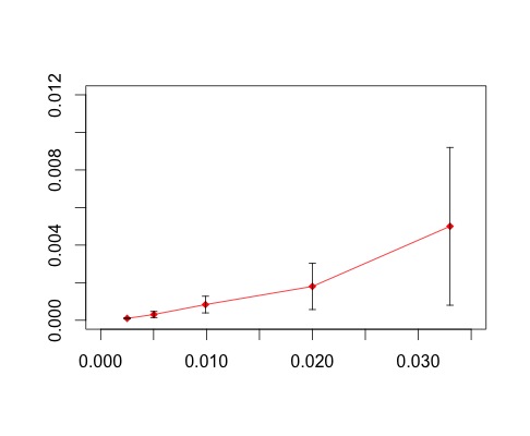
Figure 1: Mean $\pm$ 2 $\times$ standard deviation of $L_{n}$ under different $p/n$ ratios.

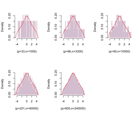
Figure 2: Histogram of the eigenvalues under five different combinations of $(p,n)$.

Next, we show the performance of the test for $H_{0}:A=A_{0};B=B_{0}$ versus $H_{1}:A=A_{1};B=B_{1}$ based on the test statistic of $L_{n}$, where $A_{j}$ and $B_{j}$, $j=0,1$ are defined in (5.1) and (5.2). Rather than performing the test at a specific level of significance, we compute the quantiles of the distribution of $L_{n}$ under $H_{0}$ and $H_{1}$ corresponding to a given set of probabilities. In order to evaluate the quantiles empirically, we simulate 500 replicates for each setting. The quantiles of the test statistics $L_{n}$ under $H_{1}$ are plotted against those under $H_{0}$ in Figure 3. Since the points lie well above the $45^{o}$ line, it shows that the test is able to reject the null hypothesis at any reasonable level of significance when the data are generated under the alternative.

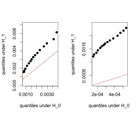
Figure 3: QQ plot of the test statistic $L_{n}$ under $H_{0}$ versus under $H_{1}$. Left panel: $p=66,n=3300$; right panel : $p=201,n=40000$.

The numerical values of the quantiles of the distribution of $L_{n}$ under $H_{0}$ and $H_{1}$ are given in Table 2. It shows that especially for $p=201$; $n=40000$ setting, the effective supports of the distributions of the test statistic are essentially separated under $H_{0}$ and $H_{1}$, indicating that the test is able to clearly discriminate between the two hypotheses.

Table 2: Quantiles of $L_{n}$ under $H_{0}$ and $H_{1}$ for $(p,n)=(66,3300)$ and $(201,40000)$.

	(66,3300)		(201,40000)
Probability	$H_{0}$	$H_{1}$	$H_{0}$	$H_{1}$
0.01	0.0008	0.0015	1.506e-4	0.0012
0.02	0.0009	0.0017	1.601e-4	0.0013
0.05	0.0010	0.0019	1.871e-4	0.0014
0.1	0.0011	0.0023	2.040e-4	0.0014
0.2	0.0013	0.0026	2.309e-4	0.0015
0.3	0.0014	0.0028	2.491e-4	0.0016
0.4	0.0015	0.0030	2.716e-4	0.0016
0.5	0.0017	0.0033	2.872e-4	0.0017
0.6	0.0019	0.0035	3.151e-4	0.0018
0.7	0.0021	0.0037	3.438e-4	0.0018
0.8	0.0023	0.0041	3.835e-4	0.0019
0.9	0.0027	0.0045	4.345e-4	0.0020
0.95	0.0030	0.0049	4.664e-4	0.0021
0.98	0.0036	0.0053	5.033e-4	0.0022
0.99	0.0039	0.0061	5.343e-4	0.0023

6 Appendix

6.1 Auxiliary lemmas

Lemma 6.1.

(Lemma 2.6 of Silverstein and Bai [26]): Let $z\in\mathbb{C}^{+}$ with $v=\Im(z)$. Let $D$ and $F$ be $n\times n$ matrices with $D$ Hermitian, and let $\mathbf{r}\in\mathbb{C}^{n}$. Then,

$$\left|\mbox{tr}\left(((D-zI)^{-1}-(D+\mathbf{r}\mathbf{r}^{*}-zI)^{-1})F\right)\right|=\left|\frac{\mathbf{r}^{*}(D-zI)^{-1}F(D-zI)^{-1}\mathbf{r}}{1+\mathbf{r}^{*}(D-zI)^{-1}\mathbf{r}}\right|\leq\frac{\parallel F\parallel}{v}~{}.$$

Lemma 6.2.

(Burkhölder’s Inequality): Let $\{X_{k}\}$ be a complex martingale difference sequence with respect to the increasing $\sigma$-field $\{\mathcal{F}_{k}\}$. Then for $p>1,$

$$\mathbb{E}\left|\sum X_{k}\right|^{p}\leq K_{p}\mathbb{E}\left(\sum|X_{k}|^{2}\right)^{p/2}.$$

Lemma 6.3.

(Lemma 8.10 of Silverstein and Bai [26]): Let $A=(a_{ij})$ be an $n\times n$ non-random matrix and $X=(x_{1},\cdots,x_{n})^{{}^{\prime}}$ be random vector of independent entries. Assume that $\mathbb{E}x_{i}=0,$ $\mathbb{E}|x_{i}|^{2}=1$ and $\mathbb{E}|x_{j}|^{l}\leq\nu_{l}$. Then for any $q\geq 2$,

$$\mathbb{E}|X^{*}AX-\mbox{tr}(A)|^{q}\leq C_{q/2}\left(\nu_{2q}\mbox{tr}(AA^{*})^{q/2}+(\nu_{4}tr(AA^{*})^{q/2})\right)$$

where $C_{q}$ is a constant depending on $p$ only.

The following lemma is a consequence of Theorem A.38 and Remark A.39 in Bai and Silverstein [1].

Lemma 6.4.

Let $\{\lambda_{k}\}_{k=1}^{n}$ and $\{\delta_{k}\}_{k=1}^{n}$ be two sets of real and let their empirical distributions be denoted by $F$ and $G$, respectively. Then, for any $\alpha>0$,

$$L^{\alpha+1}(F,G)\leq\min_{\pi}\frac{1}{n}\sum_{k=1}^{n}|\lambda_{k}-\delta_{\pi(k)}|^{\alpha},$$ (6.1)

where the minimum is taken over all permutation $\pi$ of the indices $\{1,\ldots,n\}$, and $L(F,G)$ denotes the Lévy distance between the distributions $F$ and $G$.

Lemma 6.5.

(Bernstein’s inequality): Let $X_{1},\cdots,X_{N}$ be independent centered sub-exponential random variables, and $K=\max_{i}\|X_{i}\|_{\psi_{1}}$ where $\|X\|_{\psi_{1}}=\sup_{p\geq 1}p^{-1}\left(\mathbb{E}|X|^{p}\right)^{1/p}.$ Then for every $a=(a_{1},\cdots,a_{N})\in\mathbb{R}^{N}$ and every $t\geq 0,$ we have

$$\mathbb{P}\left(\left|\sum_{i=1}^{N}a_{i}X_{i}\right|>t\right)\leq 2\exp\left\{-c\min\left(\frac{t^{2}}{K^{2}\|a\|_{2}^{2}},\frac{t}{K\|a\|_{\infty}}\right)\right\}$$

Lemma 6.6.

(Corollary 5.17 in Vershynin [30]): Let $X_{1},\cdots,X_{N}$ be independent centered sub-exponential random variables, and let $K=\max_{i}\|X_{i}\|_{\psi_{1}}$ where $\|X\|_{\psi_{1}}=\sup_{p\geq 1}p^{-1}\left(\mathbb{E}|X|^{p}\right)^{1/p}.$ Then for every $\epsilon\geq 0,$ we have

$$\mathbb{P}\left(\left|\sum_{i=1}^{N}X_{i}\right|\geq\epsilon N\right)\leq 2\exp\left\{-c\min\left(\frac{\epsilon^{2}}{K^{2}},\frac{\epsilon}{K}\right)N\right\}$$

where $c>0$ is an absolute constant.

Lemma 6.7.

(Hoeffding’s inequality : Proposition 5.10 in Vershynin [30]): Let $X_{1},\cdots,X_{N}$ be independent centered sub-gaussian random variables, and let $K=\max_{i}\|X_{i}\|_{\psi_{2}}$ where $\|X\|_{\psi_{2}}=\sup_{p\geq 1}p^{-1/2}\left(\mathbb{E}|X|^{p}\right)^{1/p}.$ THen for every $a=(a_{1},\cdots,a_{N})\in\mathbb{R}^{N}$ and every $t\geq 0,$ we have

$$\mathbb{P}\left(\left|\sum_{i=1}^{N}a_{i}X_{i}\right|\geq t\right)\leq e\cdot\exp\left\{-\frac{ct^{2}}{K^{2}\|a\|_{2}^{2}}\right\}$$

where $c>0$ is an absolute constant.

6.2 Bound on $d_{1}$ : proof of (3.12)

This is a direct application of the strategy shown in Section 3.3. We will show that $d_{1}=\frac{1}{p}\mathbb{E}\left|tr\left[\left(Y^{-1}(z)-Y_{(k)}^{-1}(z)\right)\Lambda\right]\right|\leq M/p$. To this end, we repeat the computation in (3.18). Since

$$Y(z)=\sqrt{\frac{n}{p}}(VV^{*}-\bar{b}_{n}\Lambda)=Y_{(k)}(z)+\omega_{k}e_{k}^{*}+e_{k}\omega_{k}+\tau_{kk}e_{k}e_{k}^{*}.$$ (6.2)

Let $\omega_{k}e_{k}^{*}+e_{k}\omega_{k}=\mathbf{u}_{k}\mathbf{u}_{k}^{*}-\mathbf{v}_{k}\mathbf{v}_{k}^{*}$, where $\mathbf{u}_{k}=2^{-1/2}(e_{k}+\omega_{k})$ and $\mathbf{v}_{k}=2^{-1/2}(e_{k}-\omega_{k})$. Also, define $D_{1k}=Y_{(k)}+\mathbf{u}_{k}\mathbf{u}_{k}^{*}$ and $D_{2k}=D_{1k}-\mathbf{v}_{k}\mathbf{v}_{k}^{*}$ so that $D_{1k}=D_{2k}+\mathbf{v}_{k}\mathbf{v}_{k}^{*}$. Then from (6.2) we have $Y(z)=D_{2k}+\tau_{kk}e_{k}e_{k}^{*}$. Therefore,

$$\mbox{tr}\left[\left(Y^{-1}(z)-Y_{(k)}^{-1}(z)\right)\Lambda\right]$$

$$= \mbox{tr}\left[\left(Y^{-1}(z)-(D_{2k}-zI)^{-1}\right)\Lambda\right]+\mbox{tr}\left[\left((D_{2k}-zI)^{-1}-(D_{1k}-zI)^{-1}\right)\Lambda\right]$$

$$~{}~{}~{}~{}+\mbox{tr}\left[\left((D_{1k}-zI)^{-1}-Y_{(k)}^{-1}(z)\right)\Lambda\right]$$

$$= \frac{\tau_{kk}e_{k}^{*}(D_{2k}-zI)^{-1}\Lambda(D_{2k}-zI)^{-1}e_{k}}{1+\tau_{kk}e_{k}^{*}(D_{2k}-zI)^{-1}e_{k}}+\frac{\mathbf{v}_{k}^{*}(D_{1k}-zI)^{-1}\Lambda(D_{2k}-zI)^{-1}\mathbf{v}_{k}}{1+\mathbf{v}_{k}^{*}(D_{1k}-zI)^{-1}\mathbf{v}_{k}}+\frac{\mathbf{u}_{k}^{*}Y_{(k)}^{-1}\Lambda Y_{(k)}^{-1}\mathbf{u}_{k}}{1+\mathbf{v}_{k}^{*}Y_{(k)}^{-1}(z)\mathbf{u}_{k}}.$$

According to (3.16) and Lemma 6.1, each term above is bounded by $a_{0}/v$. Thus

$$\frac{1}{p}\mathbb{E}\left|\mbox{tr}\left[\left(Y^{-1}(z)-Y^{-1}_{(k)}(z)\right)\Lambda\right]\right|\leq\frac{3a_{0}}{pv}\leq\frac{M}{p}.$$ (6.3)

So we have $d_{1}\leq M/p$.

6.3 Bound on $d_{31}$

Since

$$d_{31} = \mathbb{E}\left|-\omega_{k}^{*}Y_{(k)}^{-1}(z)\omega_{k}+\tau_{kk}+\bar{b}_{2}(n)\frac{\lambda_{k}}{p}\mbox{tr}(Y^{-1}_{(k)}(z)\Lambda_{(k)})\right|^{2}$$

$$\leq 2\mathbb{E}\left|\tau_{kk}\right|^{2}+2\mathbb{E}\left|\omega_{k}^{*}Y_{(k)}^{-1}(z)\omega_{k}-\bar{b}_{2}(n)\frac{\lambda_{k}}{p}\mbox{tr}\left[Y_{(k)}^{-1}(z)\Lambda_{(k)}\right]\right|^{2},$$

and we already have

$$\mathbb{E}|\tau_{kk}|^{2}\leq\frac{n}{p}\mathbb{E}\left|\frac{\lambda_{k}}{n}\widetilde{x}_{k}^{*}B_{n}\widetilde{x}_{k}-\bar{b}(n)\lambda_{k}\right|^{2}\leq\frac{M}{p},$$ (6.4)

to prove the claim that $d_{31}\leq M/p$, we need a bound on the expected value of the term

$$\omega_{k}^{*}Y_{(k)}^{-1}(z)\omega_{k}-\bar{b}_{2}(n)\frac{\lambda_{k}}{p}\mbox{tr}\left[Y_{(k)}^{-1}(z)\Lambda_{(k)}\right]:=d_{k}^{(2)}$$

defined in (3.8). Note that

$$d_{k}^{(2)} = \frac{n}{p}v_{k}^{*}V_{(k)}^{*}Y_{(k)}^{-1}(z)V_{(k)}v_{k}-\bar{b}_{2}(n)\frac{\lambda_{k}}{p}\mbox{tr}\left[Y_{(k)}^{-1}(z)\Lambda_{(k)}\right]$$

$$= \frac{\lambda_{k}}{p}tr\left[V_{(k)}B_{n}V_{(k)}^{*}Y_{(k)}^{-1}(z)\right]-\bar{b}_{2}(n)\frac{\lambda_{k}}{p}\mbox{tr}\left[Y_{(k)}^{-1}(z)\Lambda_{(k)}\right]+d_{k}^{(1)}$$

$$= \frac{\lambda_{k}}{pn}\sum_{i,j\neq k}(\sqrt{\lambda_{i}\lambda_{j}}\widetilde{x}_{i}^{*}B_{n}^{2}\widetilde{x}_{j})(Y_{(k)}^{-1}(z))_{ji}-\bar{b}_{2}(n)\frac{\lambda_{k}}{p}\mbox{tr}\left[Y_{(k)}^{-1}(z)\Lambda_{(k)}\right]+d_{k}^{(1)}$$

$$= \frac{\lambda_{k}}{p}\sum_{i\neq k}\lambda_{i}\left(\frac{1}{n}\widetilde{x}_{i}^{*}B_{n}^{2}\widetilde{x}_{i}-\bar{b}_{2}(n)\right)(Y_{(k)}^{-1}(z))_{ii}+\frac{\lambda_{k}}{p}\sum_{i\neq j\neq k}\sqrt{\lambda_{i}\lambda_{j}}\frac{1}{n}\widetilde{x}_{i}^{*}B_{n}^{2}\widetilde{x}_{j}(Y_{(k)}^{-1}(z))_{ji}+d_{k}^{(1)}$$

$$:= d_{k}^{(3)}+d_{k}^{(4)}+d_{k}^{(1)}.$$

In order to show $\mathbb{E}|d_{k}^{(2)}|^{2}\leq M/p$, we need to derive corresponding bounds on $\mathbb{E}|d_{k}^{(3)}+d_{k}^{(4)}|^{2}$ and $\mathbb{E}|d_{k}^{(1)}|^{2}$. Using Lemma 6.3, we have that for any $q\geq 2$

$$\mathbb{E}\left|\frac{1}{n}\widetilde{x}_{i}^{*}B_{n}^{2}\widetilde{x}_{i}-\bar{b}_{2}(n)\right|^{q} \leq C_{q}\left(3^{q/2}(n^{-2}\mbox{tr}(B_{n}^{4}))^{q/2}+\nu_{2q}n^{-q}\sum_{i=1}^{n}\lambda_{i}(B_{n})^{2q}\right)$$ (6.5)

$$\leq \frac{C_{q}^{{}^{\prime}}}{n^{q}}\left((tr(B_{n}^{4}))^{q/2}+\mbox{tr}(B_{n}^{2q})\right)$$

$$\leq \frac{C_{q}^{{}^{\prime}}}{n^{q}}\left(b_{0}^{q}(n\bar{b}_{2}(n))^{q/2}+b_{0}^{2q-2}(n\bar{b}_{2}(n))\right)$$

$$\leq C_{q}^{{}^{\prime}}\left(\frac{b_{0}^{q}(\bar{b}_{2}(n))^{q/2}}{n^{q/2}}+\frac{b_{0}^{2q-2}\bar{b}_{2}(n)}{n^{q-1}}\right)\leq\frac{M}{n^{q/2}}.$$

Thus, taking $q=2$ in (6.5) and using Cauchy-Schwarz inequality, we have

$$\mathbb{E}\left|d_{k}^{(3)}+d_{k}^{(4)}\right|^{2} = \mathbb{E}\left|\frac{\lambda_{k}}{p}\mbox{tr}\left[\left(V_{(k)}B_{n}V_{(k)}^{*}-\bar{b}_{2}(n)\Lambda_{(k)}\right)Y_{(k)}^{-1}(z)\right]\right|^{2}$$ (6.6)

$$= \frac{\lambda_{k}^{2}}{p^{2}}\mathbb{E}\left|\mbox{tr}\left[\left(\frac{1}{n}\widetilde{X}_{(k)}B_{n}^{2}\widetilde{X}_{(k)}^{*}-\bar{b}_{2}(n)I_{(k)}\right)\left(\Lambda_{(k)}^{1/2}Y_{(k)}^{-1}(z)\Lambda_{(k)}^{1/2}\right)\right]\right|^{2}$$

$$\leq \frac{a_{0}^{2}}{p^{2}}\mathbb{E}\left[\mbox{tr}\left(\frac{1}{n}\widetilde{X}_{(k)}B_{n}^{2}\widetilde{X}_{(k)}^{*}-\bar{b}_{2}(n)I_{(k)}\right)^{2}\mbox{tr}\left(\Lambda_{(k)}^{1/2}Y_{(k)}^{-1}\Lambda_{(k)}Y_{(k)}^{-1}(\bar{z})\Lambda_{(k)}^{1/2}\right)\right]$$

$$\leq \frac{a_{0}^{4}}{pv^{2}}\mathbb{E}\mbox{tr}\left(\frac{1}{n}\widetilde{X}_{(k)}B_{n}^{2}\widetilde{X}_{(k)}^{*}-\bar{b}_{2}(n)\Lambda_{(k)}\right)^{2},$$

where $I_{(k)}=I-e_{k}e_{k}^{*}$. Indeed,

$$\mathbb{E}\mbox{tr}\left(\frac{1}{n}\widetilde{X}_{(k)}B_{n}^{2}\widetilde{X}_{(k)}^{*}-\bar{b}_{2}(n)\Lambda_{(k)}\right)^{2} = \sum_{i\neq k}\mathbb{E}\left(\frac{1}{n}\widetilde{x}_{i}^{*}B_{n}\widetilde{x}_{i}-\bar{b}_{2}(n)\right)^{2}+\sum_{i\neq j\neq k}\mathbb{E}\left(\frac{1}{n}\widetilde{x}_{i}^{*}B_{n}\widetilde{x}_{j}\right)^{2}$$ (6.7)

$$\leq (p-1)\frac{M_{1}}{n}+(p-1)(p-2)\frac{M_{2}}{n}.$$

Then we have

$$\mathbb{E}\left|d_{k}^{(3)}+d_{k}^{(4)}\right|^{2}\leq\frac{a_{0}^{2}}{pv^{2}}\left((p-1)\frac{M_{1}}{n}+(p-1)(p-2)\frac{M_{2}}{n}\right)\leq\frac{pM}{n}$$ (6.8)

which goes to zero as $n\to\infty$. Next, we show that $\mathbb{E}|d_{k}^{(1)}|^{2}\leq M/p$. Since

$$d_{k}^{(1)} = \frac{n}{p}v_{k}^{*}V_{(k)}^{*}Y_{(k)}^{-1}(z)V_{(k)}v_{k}-\frac{\lambda_{k}}{p}tr\left[V_{(k)}B_{n}V_{(k)}^{*}Y_{(k)}^{-1}(z)\right]$$ (6.9)

$$= \frac{\lambda_{k}}{n}\widetilde{x}_{k}^{*}Q_{n}(z)\widetilde{x}_{k}-\mbox{tr}(Q_{n}(z))$$

where $Q_{n}(z):=B_{n}^{1/2}V_{(k)}^{*}Y_{(k)}^{-1}(z)V_{(k)}B_{n}^{1/2}$, we get

$$\mathbb{E}|d_{k}^{(1)}|^{2} = \frac{\lambda_{k}^{2}}{p^{2}}\mathbb{E}\left[\mathbb{E}\left(\left|(\widetilde{x}_{k}^{*}Q_{n}(z)\widetilde{x}_{k}-\mbox{tr}(Q_{n}(z)\right|^{2}\big{|}\widetilde{X}_{(k)}\right)\right]$$ (6.10)

$$\leq C\frac{a_{0}^{2}}{p^{2}}\mathbb{E}\mbox{tr}\left(Q_{n}(z)Q_{n}(z)^{*}\right)$$

$$\leq \frac{C^{{}^{\prime}}}{p}\mathbb{E}\|Q_{n}(z)\|^{2}$$

$$\leq \frac{M}{p}.$$

The last inequality holds due to the fact that under Gaussianity, we have

$$\|Q_{n}(z)\|^{2}\leq\|B_{n}\|^{2}\|n^{-1}\widetilde{X}_{(k)}\Lambda\widetilde{X}_{(k)}\|\|Y_{(k)}^{-1}(z)\|\leq\frac{b_{0}^{2}a_{0}}{v}\|n^{-1}\widetilde{X}_{(k)}\widetilde{X}_{(k)}^{*}\|\leq\frac{b_{0}^{2}a_{0}}{v}\|n^{-1}\widetilde{X}\widetilde{X}^{*}\|$$

so that

$$\mathbb{E}\|Q_{n}(z)\|^{2}\leq\frac{b_{0}^{2}a_{0}}{v}\mathbb{E}\|n^{-1}\widetilde{X}\widetilde{X}^{*}\|\leq\frac{b_{0}^{2}a_{0}}{v}(1+c\sqrt{p/n})\leq M.$$

Therefore, combining (6.8) and (6.10) we derive that $\mathbb{E}|d_{k}^{(2)}|\leq M/p$. This, together with (6.4), implies that $d_{31}\leq M/p$.

6.4 Bound on $d_{32}$

Denote by $\mathbb{E}_{j}(\cdot)=\mathbb{E}(\cdot|\mathcal{F}_{j})$ the conditional expectation with respect to the $\sigma$-field generated by the first $j$ rows of $X_{n}=(\mathbf{x}_{1}^{*},\cdots,\mathbf{x}_{p}^{*})^{*}$ except for $\mathbf{x}_{k}^{*}$, say, $\mathcal{F}_{j}=\sigma(\{\mathbf{x}_{l}:1\leq l\leq j,l\neq k\})$. Let $X_{(k,j)}=X_{(k)}-e_{j}\mathbf{x}_{j}^{*}$, where $e_{j}$ denotes the vector in $\mathbb{R}^{p}$ with 1 in $j$-th coordinate and zero elsewhere. Then,

$$\mbox{tr}\left[Y^{-1}_{(k)}(z)\Lambda_{(k)}\right]-\mathbb{E}\mbox{tr}\left[Y^{-1}_{(k)}(z)\Lambda_{(k)}\right]=\sum_{j\neq k}^{p}\left[\mathbb{E}_{j}\mbox{tr}\left(Y_{(k)}^{-1}(z)\Lambda_{(k)}\right)-\mathbb{E}_{j-1}\mbox{tr}\left(Y_{(k)}^{-1}(z)\Lambda_{(k)}\right)\right]:=\sum_{j\neq k}^{p}\gamma_{j}$$

where $\{\gamma_{j}\}$ forms a martingale difference sequence and can be written as

$$\gamma_{j} = \mathbb{E}_{j}\mbox{tr}\left(Y_{(k)}^{-1}(z)\Lambda_{(k)}\right)-\mathbb{E}_{j-1}\mbox{tr}\left(Y_{(k)}^{-1}(z)\Lambda_{(k)}\right)$$ (6.11)

$$= \mathbb{E}_{j}\mbox{tr}\left(Y_{(k)}^{-1}(z)\Lambda_{(k)}\right)-\mathbb{E}_{j}\mbox{tr}\left(Y_{(k,j)}^{-1}(z)\Lambda_{(k)}\right)$$

$$+ \mathbb{E}_{j-1}\mbox{tr}\left(Y_{(k,j)}^{-1}(z)\Lambda_{(k)}\right)-\mathbb{E}_{j-1}\mbox{tr}\left(Y_{(k)}^{-1}(z)\Lambda_{(k)}\right)$$

$$= (\mathbb{E}_{j}-\mathbb{E}_{j-1})\left[\mbox{tr}\left(Y_{(k)}^{-1}(z)\Lambda_{(k)}\right)-\mbox{tr}\left(Y_{(k,j)}^{-1}(z)\Lambda_{(k)}\right)\right].$$

The second equality above holds because of the fact that

$$\mathbb{E}_{j}\mbox{tr}\left(Y_{(k,j)}^{-1}(z)\Lambda_{(k)}\right)=\mathbb{E}_{j-1}\mbox{tr}\left(Y_{(k,j)}^{-1}(z)\Lambda_{(k)}\right).$$

Thus, by Lemma 6.1 we get

$$\left|\mbox{tr}\left(Y_{(k)}^{-1}(z)\Lambda_{(k)}\right)-\mbox{tr}\left(Y_{(k,j)}^{-1}(z)\Lambda_{(k)}\right)\right|\leq\frac{3a_{0}}{v}$$

and hence $|\gamma_{j}|\leq 6a_{0}/v$ by (6.11). Applying Burkhölder inequality (Lemma 6.2), we have

$$d_{32} = \mathbb{E}\left|\bar{b}_{2}(n)\frac{\lambda_{k}}{p}\mbox{tr}\left[Y^{-1}_{(k)}(z)\Lambda_{(k)}\right]-\bar{b}_{2}(n)\frac{\lambda_{k}}{p}\mathbb{E}\mbox{tr}\left[Y^{-1}_{(k)}(z)\Lambda_{(k)}\right]\right|^{2}$$

$$= \frac{(\bar{b}_{2}(n)\lambda_{k})^{2}}{p^{2}}\mathbb{E}\left|\sum_{j\neq k}\gamma_{j}\right|^{2}$$

$$\leq \frac{K}{p^{2}}\mathbb{E}\left(\sum_{j\neq k}|\gamma_{j}|^{2}\right)^{1/2}$$

$$\leq \frac{K}{p^{2}v^{2}}\left[\frac{36(p-1)a_{p}^{2}}{v^{2}}\right]^{1/2}\leq\frac{M}{p^{3/2}}.$$

6.5 Calculation on extension to non-Gaussian case

Since

$$\frac{\partial C_{n}}{\partial X_{ij}} = \frac{1}{\sqrt{np}}\lim_{\epsilon\to 0}\frac{\left(A_{p}^{1/2}(X_{n}+\epsilon\bigtriangleup_{ij})B_{n}(X_{n}+\epsilon\bigtriangleup_{ij})^{*}A_{p}^{1/2}-tr(B_{n})A_{p}\right)-\left(A_{p}^{1/2}X_{n}B_{n}X_{n}^{*}A_{p}^{1/2}-tr(B_{n})A_{p}\right)}{\epsilon}$$

$$= \frac{1}{\sqrt{np}}\left(A_{p}^{1/2}X_{n}B_{n}\bigtriangleup_{ji}A_{p}^{1/2}+A_{p}^{1/2}\bigtriangleup_{ij}B_{n}X_{n}^{*}A_{p}^{1/2}\right)$$

$$= \frac{1}{\sqrt{np}}\left(A_{p}^{1/2}X_{n}B_{n}\widetilde{e}_{j}e_{i}^{T}A_{p}^{1/2}+A_{p}^{1/2}e_{i}\widetilde{e}_{j}^{T}B_{n}X_{n}^{*}A_{p}^{1/2}\right),$$

in which $e_{i}$ is a $p\times 1$ unit vector with 1 in $i$-th coordinate and $\widetilde{e}_{i}$ is a $n\times 1$ unit vector with 1 in $i$-th coordinate. Let $r_{j}=A_{p}^{1/2}X_{n}B_{n}\widetilde{e}_{j}$ and $\xi_{i}=A_{p}^{1/2}e_{i}$. Then

$$\frac{\partial C_{n}}{\partial X_{ij}}=\frac{1}{\sqrt{np}}\left(r_{j}e_{i}^{T}A_{p}^{1/2}+A_{p}^{1/2}e_{i}r_{j}^{*}\right)=\frac{1}{\sqrt{np}}\left(r_{j}\xi_{i}^{*}+\xi_{i}r_{j}^{*}\right),$$

$$\frac{\partial^{2}C_{n}}{\partial X_{ij}^{2}}=\frac{2}{\sqrt{np}}b_{jj}A_{p}^{1/2}e_{i}e_{i}^{T}A_{p}^{1/2}=\frac{2}{\sqrt{np}}b_{jj}\xi_{i}\xi_{i}^{*},\qquad\frac{\partial^{3}C_{n}}{\partial X_{ij}^{3}}=0,$$

$$\frac{\partial^{2}G_{n}}{\partial X_{ij}^{2}}=-\frac{\partial^{2}C_{n}}{\partial X_{ij}^{2}}G^{2}_{n}+2\frac{\partial C_{n}}{\partial X_{ij}}G_{n}\frac{\partial C_{n}}{\partial X_{ij}}G^{2}_{n}=\frac{2}{\sqrt{np}}b_{jj}\xi_{i}\xi_{i}^{*}G_{n}^{2},$$

$$\frac{\partial^{3}G_{n}}{\partial X_{ij}^{3}} = -\frac{\partial^{3}C_{n}}{\partial X^{3}_{ij}}G_{n}^{2}(z)+2\frac{\partial^{2}C_{n}}{\partial X_{ij}^{2}}G_{n}\frac{\partial C_{n}}{\partial X_{ij}}G_{n}^{2}+2\frac{\partial^{2}C_{n}}{\partial X^{2}_{ij}}G_{n}\frac{\partial C_{n}}{\partial X_{ij}}G^{2}_{n}$$

$$- 2\frac{\partial C_{n}}{\partial X_{ij}}\frac{\partial C_{n}}{\partial X_{ij}}G^{2}_{n}\frac{\partial C_{n}}{\partial X_{ij}}G^{2}_{n}+2\frac{\partial C_{n}}{\partial X_{ij}}G_{n}\frac{\partial^{2}C_{n}}{\partial X_{ij}^{2}}G^{2}_{n}-4\frac{\partial C_{n}}{\partial X_{ij}}G_{n}\frac{\partial C_{n}}{\partial X_{ij}}G_{n}\frac{\partial C_{n}}{\partial X_{ij}}G^{2}_{n}$$

$$= 4\frac{\partial^{2}C_{n}}{\partial X^{2}_{ij}}G_{n}\frac{\partial C_{n}}{\partial X_{ij}}G^{2}_{n}-2\frac{\partial C_{n}}{\partial X_{ij}}\frac{\partial C_{n}}{\partial X_{ij}}G^{2}_{n}\frac{\partial C_{n}}{\partial X_{ij}}G^{2}_{n}$$

$$+2\frac{\partial C_{n}}{\partial X_{ij}}G_{n}\frac{\partial^{2}C_{n}}{\partial X_{ij}^{2}}G^{2}_{n}-4\frac{\partial C_{n}}{\partial X_{ij}}G_{n}\frac{\partial C_{n}}{\partial X_{ij}}G_{n}\frac{\partial C_{n}}{\partial X_{ij}}G^{2}_{n}.$$

So we get

$$\frac{1}{p}\mbox{tr}\left[\frac{\partial^{3}G_{n}}{\partial X_{ij}^{3}}\right]=\frac{6}{p}\mbox{tr}\left[\frac{\partial C_{n}}{\partial X_{ij}}G_{n}\frac{\partial^{2}C_{n}}{\partial X_{ij}^{2}}G_{n}^{2}\right]-\frac{6}{p}\mbox{tr}\left[\frac{\partial C_{n}}{\partial X_{ij}}G_{n}\frac{\partial C_{n}}{\partial X_{ij}}G_{n}\frac{\partial C_{n}}{\partial X_{ij}}G_{n}^{2}\right]$$

where

$$\frac{1}{p}\mbox{tr}\left[\frac{\partial C_{n}}{\partial X_{ij}}G_{n}\frac{\partial^{2}C_{n}}{\partial X_{ij}^{2}}G_{n}^{2}\right]=\frac{12b_{jj}}{np^{2}}\mbox{tr}\left[\xi_{i}^{*}G^{2}_{n}(z)(r_{j}\xi_{i}^{*}+\xi_{i}r_{j}^{*})G_{n}\xi_{i}\right]$$

and

$$\frac{1}{p}\mbox{tr}\left[\frac{\partial C_{n}}{\partial X_{ij}}G_{n}\frac{\partial C_{n}}{\partial X_{ij}}G_{n}\frac{\partial C_{n}}{\partial X_{ij}}G^{2}_{n}\right] = \frac{1}{n^{3/2}p^{5/2}}\mbox{tr}\left[(r_{j}\xi_{i}^{*}+\xi_{i}r_{j}^{*})G_{n}(r_{j}\xi_{i}^{*}+\xi_{i}r_{j}^{*})G_{n}(r_{j}\xi_{i}^{*}+\xi_{i}r_{j}^{*})G_{n}^{2}\right]$$

$$:= 2\eta_{3}(n)+2\eta_{4}(n)+2\eta_{5}(n)+2\eta_{6}(n)$$

where

$$\eta_{3}(n) = \frac{1}{n^{3/2}p^{5/2}}\left[(r_{j}^{*}G_{n}\xi_{i})^{2}r_{j}^{*}G_{n}^{2}\xi_{i}\right]$$

$$\eta_{4}(n) = \frac{1}{n^{3/2}p^{5/2}}\left[r_{j}^{*}G_{n}\xi_{i}r_{j}^{*}G_{n}r_{j}\xi_{i}^{*}G_{n}^{2}\xi_{i}\right]$$

$$\eta_{5}(n) = \frac{1}{n^{3/2}p^{5/2}}\left[r_{j}^{*}G_{n}r_{j}\xi_{i}^{*}G_{n}\xi_{i}r_{j}^{*}G^{2}_{n}\xi_{i}\right]$$

$$\eta_{6}(n) = \frac{1}{n^{3/2}p^{5/2}}\left[\xi_{i}^{*}G_{n}\xi_{i}r_{j}^{*}G_{n}\xi_{i}r_{j}^{*}G^{2}_{n}r_{j}\right].$$

6.6 Proof of Lemma 3.2

Let $B_{\cdot j}=B_{n}\widetilde{e}_{j}=(b_{1},\cdots,b_{n})^{T}$ (for brevity, dropping index $j$ on the right) and $M_{n}=A_{p}^{1/2}X_{n}$. Since $r_{j}=M_{n}B_{\cdot j}$, where $\mathbb{E}M_{ij}=0$ and $\mathbb{E}|M_{ij}|^{2}=(A_{p})_{ii}$, we have

$$\mathbb{E}\left(\|r_{j}\|^{2}\right)^{k}=\mathbb{E}\left(B_{\cdot j}^{*}M_{n}^{*}M_{n}B_{\cdot j}\right)^{k}=\mathbb{E}\left(\sum_{i=1}^{p}\left[\sum_{k=1}^{n}M_{ik}b_{k}\right]^{2}\right)^{k}=\mathbb{E}\left(\sum_{i=1}^{p}N_{i}^{2}\right)^{k},$$

where $N_{i}$, $i=1,\cdots p$, are independent, sub-Gaussian random variables with $\mathbb{E}N_{i}=0$ and $\mathbb{E}N_{i}^{2}=(A_{p})_{ii}\|B_{\cdot j}\|^{2}$. Then we have

$$\mathbb{E}\left(\sum_{i=1}^{p}N_{i}^{2}\right)^{k}=\mathbb{E}\left(\sum_{i=1}^{p}(N_{i}^{2}-\mathbb{E}N_{i}^{2})+\|B_{\cdot j}\|^{2}\mbox{tr}(A_{p})\right)^{k},$$

where $N^{2}_{i}-\mathbb{E}N^{2}_{i}$ is a mean zero sub-exponential random variable. Thus,

$$\frac{1}{p^{k}}\mathbb{E}\left(\sum_{i=1}^{p}N_{i}^{2}\right)^{k}=\mathbb{E}\left(\frac{1}{p}\sum_{i=1}^{p}(N_{i}^{2}-\mathbb{E}N_{i}^{2})+\|B_{\cdot j}\|^{2}\frac{\mbox{tr}(A_{p})}{p}\right)^{k}=O(1).$$

The term $\|B_{\cdot j}\|^{2}\mbox{tr}(A_{p})/p\leq a_{0}b^{2}_{0}=O(1)$. On the other hand, $\frac{1}{p}\sum_{i=1}^{p}(N_{i}^{2}-\mathbb{E}N^{2}_{i})$ is the average independent sub-exponential random variables with mean zero and uniformly bounded sub-exponential norm (can be verified). So by Bernstein’s inequality (Lemma 6.5), the tail probability can be controlled adequately so that $\mathbb{E}(\frac{1}{p}\sum_{i=1}^{p}(N_{i}^{2}-\mathbb{E}N^{2}_{i}))^{k}=O(1)$ for any $k\geq 1$. Hence (3.39) holds.

References

• [1] Bai, Z. D. and Silverstein, J. W. (2009). Spectral Analysis of Large Dimensional Random Matrices. Springer.
• [2] Bai, Z. D. and Silverstein, J. W. (1999). Exact separation of eigenvalues of large dimensional sample covariance matrices. Annals of Probability, 27, 1536–1555.
• [3] Bai, Z. D. and Yin, Y. Q. (1988). Convergence to the semicircle law. Annals of Probility, 16, 863–875.
• [4] Bai, Z. D. and Zhang, L. X. (2010). The limiting spectral distribution of the product of the Wigner matrix and a nonnegative definite matrix. Journal of Multivariate Analysis, 101, 1927–1949.
• [5] Bao, Z. G. (2012). Strong convergence of ESD for the generalized sample covariance matrices when $p/n\to 0$. Statistical and Probability letters, 82, 894–901.
• [6] Chatterjee, S. (2006). A generalization of Lindeberg principle. Annals of Probability, 6, 2061–2076.
• [7] Dutilleul, P. (1999). The MLE algorithm for the matrix normal distribution. Journal of Statistical Computation and Simulation, 64, 105–123.
• [8] Eaton, M. L. and Tyler, D. E. (1991). On Weilandt’s inequality and its application to the asymptotic distribution of the eigenvalues of a random symmetric matrix. Annals of Statistics, 19, 260–271.
• [9] El Karoui, N. (2009). Concentration of measure and spectra of random matrices : Applications to correlation matrices, elliptical distributions and beyond. Annals of Applied Probability, 19, 2362–2405.
• [10] Fuentes, M. (2006). Testing separability of spatio-temporal covariance functions. Journal of Statistical Planning and Inference, 136, 447–466.
• [11] Kyriakidis, P. and Journel, A. G. (1999). Geostatistical space-time models : a review. Mathematical Geology, 31, 651–684.
• [12] McDiarmid, C. (1989). On the method of bounded differeces. Surveys in Combinatorics 141, 148–188.
• [13] Mitchell, M. W. and Gumpertz, M. L. (2003). Spatial variability inside a free-air CO2 enrichment system. Journal of Agricultural, Biological, and Environmental Statistics,
• [14] Mitchell, M. W., Genton, M. G. and Gumpertz, M. L. (2005). Testing for separability of space-time covariances. Environmetrics, 16, 819–831.
• [15] Mitchell, M. W., Genton, M. G. and Gumpertz, M. L. (2006). A likelihood ratio test for separability of covariances. Journal of Multivariate Analysis 97, 1025–1043.
• [16] Ledoux, M. (2003). The Concentration of Measure Phenomenon. American Mathematical Society.
• [17] Li, B., Genton, M. G. and Sherman, M. (2008). Testing the covariance structure of multivariate random fields. Biometrika, 95, 813–829.
• [18] Lu, N. and Zimmerman, D. L. (2005). The likelihood ratio test for a separable covariance matrix. Statistics and Probability letters, 73, 449–457.
• [19] Pastur, L. and Shcherbina, M. (2011). Eigenvalue Distribution of Large Random Matrices. American Mathematical Society.
• [20] Pan, G. M. and Gao, J. T. (2009). Asymptotic theory for sample covariance matrix under cross-sectional dependence. Manuscript.
• [21] Paul, D. (2007). Asymptotics for sample eigenstructure for a large dimensional spiked covariance model. Statistica Sinica, 17, 1617–1642.
• [22] Paul, D. and Aue, A. (2013). Random matrix theory in statistics : a review. Manuscript.
• [23] Paul, D. and Silverstein, J. W. (2009). No eigenvalues outside the support of a separable covariance matrix. Journal of Multivariate Analysis, 100, 37–57.
• [24] Roy, A. and Khatree, R. (2005) On implementation of a test for kronecker product covariance structure for multivariate repeated measures data. Statistical Methodology, 2, 297–306.
• [25] Rudelson, M. and Vershynin, R. (2013). Hanson-Wright inequality and sub-Gaussian concentration. arXiv:1306.2872.
• [26] Silverstein, J. W. and Bai, Z. D. (1995), On the empirical distribution of eigenvalues of a class of large dimensional random matrices. Journal of Multivariate Analysis, 54, 175–192.
• [27] Silverstein, J. W. and Choi, S. I. (1995). Analysis of the limiting spectral distribution of large dimensional random matrices. Journal of Multivariate Analysis, 54, 175–192.
• [28] Simpson, S. L. (2010). An adjusted likelihood ratio test for separability in unbalanced multivariate repeated measures data. Statistical Methodology, 7, 511–519.
• [29] Stewart, G. W. (1980). The efficient generation of random orthogonal matrices with an application to condition estimators. SIAM Journal of Numerical Analysis, 71, 403–409.
• [30] Vershynin, R. (2010). Introduction to the non-asymptotic analysis of random matrices. arXiv preprint:1011.3027
• [31] Zhang, L. X. (2006). Spectral Analysis of Large Dimensional Random Matrices. Ph.D. thesis. National University of Singapore.