Explicit Formula of Energy-Conserving Fokker-Planck Type Collision Term for Single Species Point Vortex Systems with Weak Mean Flow

Abstract

This paper derives a kinetic equation for a two-dimensional single species point vortex system. We consider a situation (different from the ones considered previously) of weak mean flow where the time scale of the macroscopic motion is longer than the decorrelation time so that the trajectory of the point vortices can be approximated by a straight line on the decorrelation time scale. This may be the case when the number $N$ of point vortices is not too large. Using a kinetic theory based on the Klimontovich formalism, we derive a collision term consisting of a diffusion term and a drift term, whose structure is similar to the Fokker-Planck equation. The collision term exhibits several important properties: (a) it includes a nonlocal effect; (b) it conserves the mean field energy; (c) it satisfies the $H$ theorem; (d) its effect vanishes in each local equilibrium region with the same temperature. When the system reaches a global equilibrium state, the collision term completely converges to zero all over the system. The theoretical prediction of the relaxation time of the system from the obtained kinetic equation is confirmed by direct numerical simulations of point vortices.

I Introduction

The two-dimensional (2D) microscopic point vortex system Newton (2001) is a formal solution of the 2D inviscid microscopic Euler equation,

$$\frac{\partial}{\partial t}\hat{\omega}(\bm{r},t)+\nabla\cdot(\hat{\bm{u}}(\bm{r},t)\hat{\omega}(\bm{r},t))=0,$$ (1)

where $\hat{\omega}(\bm{r},t)$ and $\hat{\bm{u}}(\bm{r},t)$ are the microscopic vorticity and the microscopic velocity, respectively. Equation (1) is formally identical to the macroscopic Euler equation

$$\frac{\partial}{\partial t}\omega(\bm{r},t)+\nabla\cdot(\bm{u}(\bm{r},t)\omega(\bm{r},t))=0,$$ (2)

where $\omega(\bm{r},t)$ and $\bm{u}(\bm{r},t)$ are the macroscopic vorticity and the macroscopic velocity, respectively. The point vortex system has been successfully applied to the study of 2D turbulence Kraichnan and Montgomery (1980); Tabeling (2002). In the landmark paper published in 1949, Onsager proposed an application of statistical mechanics to the 2D point vortex system, in which he sketched a possible explanation for the formation of large-scale, long-lived, vortex structures in turbulent flows Onsager (1949); Eyink and Sreenivasan (2006). Negative temperature equilibrium states described by the Boltzmann distribution (leading to the sinh-Poisson equation when considering the two-species point vortex system) are found by Joyce and Montgomery Joyce and Montgomery (1973). Since then, a large research effort has been devoted to understand the negative temperature states, both theoretically and numerically Montgomery and Joyce (1974); Kida (1975); Kraichnan (1975); Seyler, Jr. (1976); Pointin and Lundgren (1976); Lundgren and Pointin (1977); Ting et al. (1987); Robert and Sommeria (1991); Eyink and Spohn (1993); Bühler (2002); Yatsuyanagi et al. (2005); Chavanis (2002). On the other hand, it has been pointed out that a decaying 2D Navier-Stokes turbulence reaches an equilibrium state described by the sinh-Poisson equation Matthaeus et al. (1991); Montgomery et al. (1992); Li and Montgomery (1996).

Here, a question arises. A distribution of the point vortices $\hat{\omega}(\bm{r},0)$ is given at $t=0$. A time-evolved distribution $\hat{\omega}(\bm{r},T)$ at a certain time $T$ is obtained by solving the microscopic Euler equation (1). On the other hand, a macroscopic vorticity field $\omega(\bm{r},0)$ at $t=0$ is obtained by a space average of $\hat{\omega}(\bm{r},0)$, namely $\omega(\bm{r},0)=\langle\hat{\omega}(\bm{r},0)\rangle$. Of course, a time-evolved macroscopic vorticity field $\omega(\bm{r},T)$ is obtained by solving the macroscopic Euler equation (2). Is the space-averaged point vortex solution $\langle\hat{\omega}(\bm{r},T)\rangle$ the same as the macroscopic vorticity field $\omega(\bm{r},T)$? If the number of point vortices $N\rightarrow+\infty$, the answer is “yes” because there is no fluctuation about the mean field Note01 . By contrast, for finite $N$ systems, the answer is “no” because there are fluctuations implying a deviation to the macroscopic Euler equation. In that case, the evolving equation for $\omega(\bm{r},{t})$ which is exactly equal to $\langle\hat{\omega}(\bm{r},{t})\rangle$ should be written as

$$\frac{\partial\omega(\bm{r},t)}{\partial t}+\nabla\cdot(\bm{u}(\bm{r},t)\omega(\bm{r},t))=C,$$ (3)

where $C$ is a collision term. In the following, we restrict our discussion to determining an explicit formula of $C$, i.e., we develop a kinetic theory of point vortices.

The kinetic theory of point vortices has attracted a lot of attention. Let us briefly review earlier works on the subject. A general kinetic equation for point vortices, valid for arbitrary flows (axisymmetric or not), has been obtained by Chavanis Chavanis (2001, 2008) with several equivalent methods (projection operator technics, the BBGKY hierarchy, and the Klimontovich approach). It writes Note02

$$\frac{\partial\omega(\bm{r},t)}{\partial t}+\nabla\cdot(\bm{u}(\bm{r},t)\omega(\bm{r},t))=\frac{\partial}{\partial{r}^{\mu}}\int_{0}^{+\infty}d\tau\int d\bm{r}_{1}{V}^{\mu}(1\rightarrow 0)G(t,t-\tau)$$

$$\times\left[{{\tilde{V}}}^{\nu}(1\rightarrow 0){\partial\over\partial{r}^{\nu}}+{{\tilde{V}}}^{\nu}(0\rightarrow 1){\partial\over\partial{r}_{1}^{\nu}}\right]{\omega}(\bm{r},t)\frac{\omega}{\Omega}(\bm{r}_{1},t),$$ (4)

where $G(t,t-\tau)$ is a Green function constructed with the mean velocity, $\bm{V}(i\rightarrow j)$ is the velocity created by point vortex $i$ on point vortex $j$, $\tilde{\bm{V}}(i\rightarrow j)$ is the fluctuating velocity, and $\Omega$ is the circulation of a point vortex. This equation is valid at the order $O(1/N)$ when $N\rightarrow+\infty$, so it describes the evolution of the system of point vortices, due to two-body distant encounters, on a time scale of the order $Nt_{D}$ where $t_{D}$ is the dynamical time. For axisymmetric flows, the point vortices have a circular motion with angular velocity $\Omega(r,t)$. In that case, the collision term can be simplified and the kinetic equation (4) takes the form Chavanis (2001, 2008):

$$\frac{\partial\omega(r,t)}{\partial t}=-\frac{\Omega}{4}\frac{1}{r}\frac{\partial}{\partial r}\int_{0}^{+\infty}r^{\prime}\,dr^{\prime}\ln\left[1-\left(\frac{r_{<}}{r_{>}}\right)^{2}\right]\delta(\Omega(r,t)-\Omega(r^{\prime},t))$$

$$\times\left(\frac{1}{r}\frac{\partial}{\partial r}-\frac{1}{r^{\prime}}\frac{\partial}{\partial r^{\prime}}\right)\omega(r,t)\omega(r^{\prime},t).$$ (5)

This equation conserves circulation, energy, angular momentum, and it increases monotonically the Boltzmann entropy ($H$ theorem). The collisional evolution of the point vortices is due to a condition of resonance encapsulated in the $\delta$-function. We note that when the profile of angular velocity is, or becomes, monotonic, the condition of resonance cannot be satisfied anymore and the collision term vanishes. As a result, the evolution described by the kinetic equation (I) stops even if the attained distribution differs from the Boltzmann distribution (this is because the kinetic equation (I) admits an infinity of steady states in addition to the Boltzmann distribution, namely any distribution with a monotonic profile of angular velocity). Therefore, the kinetic equation (I) usually does not converge towards the Boltzmann distribution Chavanis and Lemou (2007). This is not a problem. It simply tells us that, for axisymmetric flows, the relaxation towards the Boltzmann distribution is governed by another kinetic equation, valid at the order $1/N^{2}$ (or at a higher order), taking into account more complicated correlations between point vortices than simply two-body collisions. As a result, the relaxation time towards the Boltzmann distribution is of order $N^{2}t_{D}$ or longer Chavanis (2012a, b); Chavanis and Lemou (2007); Chavanis (2010). It is also possible that the point vortex gas (in the axisymmetric situation) never achieves the Boltzmann distribution. This is still an open problem. For non-axisymmetric flows, a natural strategy would be to introduce angle-action variables to obtain a generalization of the kinetic equation (I) similarly to what has been done in the context of the Landau and Lenard-Balescu equations in stellar dynamics Chavanis (2010); Heyvaerts (2010); Chavanis (2012c, 2013). Alternatively, Chavanis Chavanis (2001, 2008) has proposed a heuristic simplification of the kinetic equation (4) in the form

$$\frac{\partial{\omega}}{\partial t}+{\bm{u}}\cdot\nabla{\omega}=\frac{\Omega}{8}\nabla\cdot\int d\bm{r}^{\prime}\,\frac{\bm{x}_{\perp}\otimes\bm{x}_{\perp}}{x^{2}}\delta({\bm{x}}\cdot{\bm{w}})\left({\omega}^{\prime}\nabla{\omega}-{\omega}\nabla^{\prime}{\omega}^{\prime}\right),$$ (6)

where $\omega=\omega(\bm{r},t)$, $\omega^{\prime}=\omega(\bm{r}^{\prime},t)$, $\bm{x}=\bm{r}-\bm{r}^{\prime}$, and $\bm{w}=\bm{u}(\bm{r},t)-\bm{u}(\bm{r}^{\prime},t)$. This equation conserves circulation, energy, angular momentum, and it increases monotonically the Boltzmann entropy ($H$ theorem). Furthermore, for axisymmetric flows, it reduces to a form very close to the exact Eq. (I) up to logarithmic corrections. As in Eq. (I), the collisional evolution of the point vortices according to Eq. (6) is due to a condition of resonance encapsulated in the $\delta$-function. However, this condition of resonance is more complicated (hence more easily satisfied) than in Eq. (I) so we may expect that the solution of this equation reaches, or approaches, the Boltzmann distribution on the time scale $Nt_{D}$ over which this equation is valid. Indeed, there are numerical observations that, for non-axisymmetric flows, the relaxation time is of order $Nt_{D}$ Kawahara and Nakanishi (2007). Therefore, if there are enough resonances, the kinetic equation (6) will drive the system towards the Boltzmann distribution on a time scale $Nt_{D}$ while if the resonances cannot be satisfied the kinetic equation (6) is not sufficient to describe the dynamics (we have to take terms of order $1/N^{2}$, or higher, into account) and the relaxation time will be of order $N^{2}t_{D}$, or longer Chavanis (2012a, b); Chavanis and Lemou (2007); Chavanis (2010). As discussed in Refs. Chavanis (2001, 2008), the kinetic equations (4)-(6) have the form of Fokker-Planck equations

$$\frac{\partial{\omega}}{\partial t}+\bm{u}\cdot\nabla{\omega}=\nabla\cdot({\sf D}\cdot\nabla\omega-\omega\bm{V}),$$ (7)

including a diffusion term and a drift term (they exactly reduce to Fokker-Planck equations in the test particle approach). The drift term was first evidenced in Ref. Chavanis (1998) and it plays a fundamental role in the kinetic theory of point vortices in relation to the process of self-organization. Finally, these kinetic equations can be easily generalized to the multi-species point vortex gas as discussed in Refs. Dubin (2003); Chavanis and Lemou (2007).

In the previous kinetic theories Chavanis (2001, 2008); Dubin and O’Neil (1988); Dubin (2003); Chavanis (2010, 2012a, 2012b); Chavanis and Lemou (2007); Chavanis (1998), the mean field is assumed to be “strong” and the fluctuations “weak” so that the point vortices are advected by the mean velocity for a long time. For example, in an axisymmetric flow, the point vortices follow circular trajectories in a first approximation slightly perturbed by the effect of the long-range collisions (whose strength is of order $|\delta{\bm{u}}|\sim 1/\sqrt{N}$) on a very long time scale. In that case, the dynamics of the point vortices is “resonant” (see the $\delta$-function in Eqs. (I) and (6)). The opposite situation is when there is no mean flow. This is the situation investigated by Taylor and McNamara Taylor and McNamara (1971) and Dawson and collaborators Dawson et al. (1971); Okuda and Dawson (1973). They consider a neutral system of point vortices at equilibrium where the vortices are uniformly distributed in average. In that case, there is no kinetic equation for $\omega(\bm{r},t)$ since $\omega(\bm{r},t)=0$ at each time $t$ (however, there can be large-scale fluctuations giving rise to Dawson vortices). Taylor and McNamara Taylor and McNamara (1971) consider the diffusion of a test vortex in a uniform vorticity background where the field vortices can be correlated (having a thermal distribution) or uncorrelated (having a random distribution) and derive the corresponding diffusion coefficient. In that case, there is no drift since the vorticity is uniform. In the present paper, we consider a situation intermediate between the works of Refs. Chavanis (2001, 2008); Dubin and O’Neil (1988); Dubin (2003); Chavanis (2010, 2012a, 2012b); Chavanis and Lemou (2007); Chavanis (1998) and the works of Refs. Taylor and McNamara (1971); Dawson et al. (1971); Okuda and Dawson (1973). We assume that the mean field is weak, but non-zero, so the time scale of the macroscopic motion is long as compared to the decorrelation time. In this case, we can make a linear trajectory approximation with the local velocity field ${\bm{u}}({\bm{r}},t)$ to compute the correlation function. In our problem, the distribution of the point vortices is spatially inhomogeneous and out of equilibrium, so our aim is to determine a kinetic equation that describes the relaxation of $\omega(\bm{r},t)$ towards the Boltzmann distribution. Since the mean flow is weak, the kinetic evolution will not be “resonant” so it should be described by a kinetic equation different from Eqs. (I) and (6). This approach is not in contradiction with previous works. It just explores a completely different regime, so it should be considered as being complementary to previous works Note03 . In Appendix A, we try to justify the domain of validity of this approach by estimating the decorrelation time and the time scale of the macroscopic motion. It is shown that there is a critical value of $N_{c}$. The case of $1\ll N\ll N_{c}$ corresponds to the situation of the current paper and the case of $N\gg N_{c}$ corresponds to the previous studies. However, we make clear since the start that the present approach is not firmly justified mathematically (in a well-defined asymptotic limit) and this is the reason of the problems encountered, and discussed, at the end of the paper. Despite these limitations, the linear trajectory approximation is interesting in itself because it makes the kinetic theory very similar to that developed in plasma physics and stellar dynamics where the particles have linear trajectories due to their inertia. Therefore, it is interesting to see what a similar approximation implies in the case of point vortices. Furthermore, it leads to explicit kinetic equations that could be confronted to direct numerical simulations. Actually, this linear trajectory approximation was introduced in Appendix B of Ref. Chavanis (2008) where the kinetic equation (57) was derived directly from Eq. (4). For self-consistency, this equation is re-derived here from the start by using the Klimontovich formalism. Then, we introduce a space average of the diffusion flux and derive the kinetic equation (68). The obtained collision term has the following good properties. (i) It conserves the mean field energy. (ii) During the relaxation process towards the global equilibrium, the system first reaches a local equilibrium state. In the local equilibrium state, the relation $\omega_{\rm leq}=\omega_{\rm leq}[\psi]$ is satisfied in each small region inside which the inverse temperature $\beta$ is constant (notation $\omega[\psi]$ is a functional of the stream function $\psi$). In the small regions, the second term $\nabla\cdot(\bm{u}\omega)$ of the Euler equation (3) vanishes. Then the time evolution of the system is dominated by the collision term. However, the magnitude of the collision term is small compared to that of $\nabla\cdot(\bm{u}\omega)$, and the speed of the relaxation slows down. When the system reaches a global equilibrium state described by the Boltzmann distribution $\omega_{\rm eq}=\omega_{0}\exp(-\beta\Omega\psi_{\rm eq})$, the collision term completely converges to zero all over the system and the Einstein relation is obtained Chavanis (2001). (iii) The obtained collision term satisfies the $H$ theorem which guarantees that the system relaxes to a global equilibrium state. As the order of the collision term is $O(1/N)$, the relaxation time scales as $N$.

In order to illustrate our theoretical study, we have performed direct numerical simulations of point vortices to confirm the scaling of the relaxation time. The results elucidate a new scaling according to which the relaxation time $t_{R}$ is proportional to $1/\Omega$. The previously obtained scaling $t_{R}\propto Nt_{D}$ by Kawahara and Nakanishi Kawahara and Nakanishi (2007) where $t_{D}$ is the dynamical time of the system is also reexamined and confirmed.

The organization of this paper is as follows. In Sec. II, the point vortex system and the Klimontovich formalism are briefly introduced. In Sec. III, we demonstrate explicit formulae for the diffusion and the drift terms as intermediate results. In Sec. IV, a detailed calculation of the diffusion term is shown. Since similar calculations can be applied to the drift term, the details for the drift term are omitted. In Sec. V, three good properties of the collision term are demonstrated. In Sec. VI, we mention the limitation of our approach. Finally, in Sec. VII, we compare our results with direct numerical simulations of point vortices. We find a good qualitative agreement.

II Point Vortex System

Consider a 2D system consisting of $N$ positive point vortices Newton (2001). The circulation of each point vortex is given by a positive constant $\Omega$. Therefore,

$$\hat{\omega}=\sum_{i}^{N}\Omega\delta(\bm{r}-\bm{r}_{i}),$$ (8)

where $\hat{\omega}=\hat{\omega}(\bm{r},t)$ is the $z$-component of the microscopic vorticity on the $x-y$ plane, and $\delta(\bm{r})$ is the Dirac delta function in two dimensions. The microscopic variables in the microscopic equation are identified by $\hat{\cdot}$. For brevity, we shall omit the $t$ and $\bm{r}$ dependences if there is no ambiguity. Vector $\bm{r}_{i}=\bm{r}_{i}(t)$ is the position vector of the $i$-th point vortex. The discretized vorticity (8) is a formal solution of the microscopic Euler equation (1). Other microscopic variables are defined by

$$\hat{\bm{u}}=\hat{\bm{u}}(\bm{r},t)=-\hat{\bm{z}}\times\nabla\hat{\psi},$$ (9)

$$\hat{\psi}=\hat{\psi}(\bm{r},t)=\sum_{i}\Omega_{i}G(\bm{r}-\bm{r}_{i}),$$ (10)

$$G(\bm{r})=-\frac{1}{2\pi}\ln|\bm{r}|,$$ (11)

where $\hat{\bm{u}}$ and $\hat{\psi}$ are the velocity field and the stream function in the 2D plane, $\hat{\bm{z}}$ is the unit vector in the $z$-direction, and $G(\bm{r})$ is the 2D Green function for the Laplacian operator in an infinite domain. Since the solution of a macroscopic fluid equation should be given by a smooth function, the singular solution (8) should be regarded not as a solution of the macroscopic equation but as one of the microscopic equation. Thus we call the equation that has the microscopic point vortex solution (8), the “microscopic” Euler equation.

There exist many analogies between point vortices, plasmas, and stellar systems (despite, of course, some important differences), and similar methods can be developed to study these systems Chavanis (2002). In plasma physics and stellar dynamics, the evolution of the macroscopic phase space density $f({\bm{r}},{\bm{v}},t)$ is governed by the Vlasov-Landau kinetic equation

$$\frac{\partial f}{\partial t}+\bm{v}\cdot\nabla_{\bm{r}}f+\bm{F}\cdot\nabla_{\bm{v}}f=A\frac{\partial}{\partial v_{i}}\int d\bm{v}^{\prime}\frac{w^{2}\delta_{ij}-w_{i}w_{j}}{w^{3}}\left(f^{\prime}\frac{\partial f}{\partial v_{j}}-f\frac{\partial f^{\prime}}{\partial v^{\prime}_{j}}\right),$$ (12)

where $f=f(\bm{r},\bm{v},t)$, $f^{\prime}=f(\bm{r},\bm{v}^{\prime},t)$, $\bm{w}=\bm{v}-\bm{v}^{\prime}$, $\bm{F}(\bm{r},t)$ is the mean force by unit of mass acting on a particle, and $A$ is a constant ($A=2\pi mG^{2}\ln\Lambda$ for stellar systems and $A=(2\pi e^{4}/m^{3})\ln\Lambda$ for plasmas where $\ln\Lambda$ is the Coulombian logarithm). This equation can be derived from the Klimontovich equation for the microscopic phase space density $\hat{f}$ that is

$$\frac{\partial\hat{f}}{\partial t}+\bm{v}\cdot\nabla_{\bm{r}}\hat{f}+\hat{\bm{F}}\cdot\nabla_{\bm{v}}\hat{f}=0$$ (13)

by using a quasilinear approximation Klimontovich (1967). The Vlasov-Landau equation has the form of a Fokker-Planck equation

$$\frac{\partial f}{\partial t}+\bm{v}\cdot\nabla_{\bm{r}}f+\bm{F}\cdot\nabla_{\bm{v}}f=\nabla_{\bm{v}}\cdot({\sf D}\cdot\nabla_{\bm{v}}f-f\bm{A}),$$ (14)

including a diffusion term and a friction (it exactly reduces to a Fokker-Planck equation in the test particle approach). As the dynamics of plasmas and stellar systems is usually dominated not by collisions but by a collective behavior due to long-range interactions, the collision term can often be neglected (on a collisionless time scale or for $N\rightarrow+\infty$) and it yields the simplest form of the kinetic equation called the Vlasov equation:

$$\frac{\partial f}{\partial t}+\bm{v}\cdot\nabla_{\bm{r}}f+\bm{F}\cdot\nabla_{\bm{v}}f=0.$$ (15)

The same hierarchy exists in the 2D fluid equations Chavanis (2002). The most microscopic equation is the microscopic Euler equation (1), which has the discrete particle solution (8). This is the counterpart of the Klimontovich equation (13) in plasma physics and stellar dynamics. Dividing the microscopic variables into a macroscopic and a fluctuation part, and taking ensemble average yields a macroscopic fluid equation with a collisional effect like the kinetic equations (4)-(6) derived in the past or like the kinetic equation (68) derived in this paper. These kinetic equations are analogous to the Vlasov-Landau equation (12). They have a Fokker-Planck form in which the drift of the point vortices is the counterpart of the dynamical friction [compare Eqs. (7) and (14)], as noted in Ref. Chavanis (1998). Ignoring the collision term in the above macroscopic equations, we obtain the inviscid fluid equation, namely the macroscopic Euler equation (2). This is the counterpart of the Vlasov equation (15). These analogies were first pointed out in Ref. Chavanis (2002).

The starting equation is the microscopic Euler equation (1). Inserting the following expressions into Eq. (1),

$$\hat{\omega} = \omega+\delta\omega,$$ (16)

$$\hat{\bm{u}} = \bm{u}+\delta\bm{u},$$ (17)

and taking the ensemble average, we obtain the following macroscopic equation with the collision term $C=C(\bm{r},t)$

$$\frac{\partial\omega}{\partial t}+\nabla\cdot(\bm{u}\omega)=C,$$ (18)

where

$$C\equiv-\nabla\cdot\bm{\Gamma}(\bm{r},t),$$ (19)

$$\bm{\Gamma}=\langle\delta\bm{u}\delta\omega\rangle=-\int d\bm{r}^{\prime}\bm{F}(\bm{r}-\bm{r}^{\prime})\langle\delta\omega^{\prime}\delta\omega\rangle,$$ (20)

$$\bm{F}(\bm{r})=\hat{\bm{z}}\times\nabla G(\bm{r}),$$ (21)

where $\bm{\Gamma}$ denotes a diffusion flux. We note $\delta\omega^{\prime}$ for $\delta\omega(\bm{r}^{\prime},t)$. Similarly, we shall note $\omega^{\prime}$ for $\omega(\bm{r}^{\prime},t)$. To obtain Eq. (20), the following relation has been utilized

$$\delta\bm{u}=-\int d\bm{r}^{\prime}\bm{F}(\bm{r}-\bm{r}^{\prime})\delta\omega^{\prime}.$$ (22)

In the next section, we will analytically assess the collision term $C$ in the case where a linear trajectory approximation can be implemented.

III Evaluation of Collision Term

We consider a point vortex system with large $N$ keeping the total circulation $N\Omega$ constant. Therefore, $\Omega\sim 1/N$. We expect that the collision term $C$ appearing in Eq. (18) for the point vortex system has two terms, a diffusion term proportional to $\nabla\omega$ and a drift term proportional to $\omega$, namely

$$\bm{\Gamma}\equiv-{\sf D}\cdot\nabla\omega+\bm{V}\omega,$$ (23)

where ${\sf D}={\sf D}(\bm{r},t)$ is a diffusion tensor and $\bm{V}=\bm{V}(\bm{r},t)$ is a drift velocity. To evaluate $\sf D$ and $\bm{V}$ explicitly, we assume there exist a small parameter $\epsilon$ such that:

$$\omega\approx\nabla^{2}\psi\approx O(\epsilon^{0}),\quad\bm{u}\approx\nabla\psi\approx O(\epsilon^{0}),\quad\nabla\bm{u}\approx\nabla^{2}\psi\approx O(\epsilon^{0}),$$

$$\nabla\omega\approx O(\epsilon^{1/2}),\quad\delta\omega\approx O(\epsilon^{1/2}),\quad\delta\bm{u}\approx O(\epsilon^{1/2}),$$

$$\frac{\partial\bm{u}}{\partial t}\approx O(\epsilon^{1/2}),\quad\frac{\partial\omega}{\partial t}\approx O(\epsilon^{1/2}),\quad\nabla\nabla\bm{u}\approx O(\epsilon^{1/2}),$$

$$\bm{\Gamma}\approx O(\epsilon).$$ (24)

The expansion parameter $\epsilon$ is similar to the one introduced by Chavanis in Refs. Chavanis (2001, 2008, 2012a) and the references therein. However, we assume here that the gradient of the vorticity profile is weak. This is necessary for the validity of the linear trajectory approximation. With this scaling, the left hand side of Eq. (18) is $O(\epsilon^{1/2})$, while the right hand side is $O(\epsilon^{3/2})$. Expressing $\sf D$ and $\bm{V}$ in the form of a perturbation expansion and gathering the terms of the appropriate order, an analytical formula for the collision term $C$ will be obtained.

To rewrite the collision term in Eq. (18) according to the above prospect, we introduce a linearized equation obtained by inserting Eqs. (16) and (17) into Eq. (1) and assembling the first-order fluctuation terms:

$$\frac{\partial}{\partial t}\delta\omega+\nabla\cdot(\bm{u}\delta\omega)=-\delta\bm{u}\cdot\nabla\omega.$$ (25)

This is the counterpart of the quasilinear approximation in plasma physics Klimontovich (1967). As the macroscopic quantities $\bm{u}$ appearing in the second term in the left-hand side and $\nabla\omega$ in the right-hand side are supposed to be constant in the time scale of the microscopic fluctuation, Eq. (25) can be integrated:

$$\delta\omega = -\int_{t_{0}}^{t}d\tau\delta\bm{u}(\bm{r}-\bm{u}(t-\tau),\tau)\cdot\nabla\omega$$ (26)

$$+\delta\omega(\bm{r}-\bm{u}(t-t_{0}),t_{0}),$$

$$\delta\omega^{\prime} = -\int_{t_{0}}^{t}d\tau\delta\bm{u}(\bm{r}^{\prime}-\bm{u}^{\prime}(t-\tau),\tau)\cdot\nabla^{\prime}\omega^{\prime}$$ (27)

$$+\delta\omega(\bm{r}^{\prime}-\bm{u}^{\prime}(t-t_{0}),t_{0}),$$

where $\nabla^{\prime}\omega^{\prime}=\nabla_{\bm{r}^{\prime}}\omega(\bm{r}^{\prime})$. This is called the linear trajectory approximation where the trajectory of the point vortex is straight. The validity of this approximation is discussed in Appendix A. The value of $t_{0}$ is chosen to satisfy $t-t_{0}\gg t_{c}$ where $t_{c}$ is a correlation time of the fluctuations. Substituting Eqs. (26) and (27) into the correlation term in Eq. (20), we obtain

$$\left\langle\delta\omega^{\prime}\delta\omega\right\rangle$$ (30)

$$= \left\langle\left(-\int_{t_{0}}^{t}d\tau\delta\bm{u}(\bm{r}^{\prime}-\bm{u}^{\prime}(t-\tau),\tau)\cdot\nabla^{\prime}\omega^{\prime}\right)\right.$$

$$\times\left.\left(-\int_{t_{0}}^{t}d\tau\delta\bm{u}(\bm{r}-\bm{u}(t-\tau),\tau)\cdot\nabla\omega\right)\right\rangle$$

$$+\left\langle\left(-\int_{t_{0}}^{t}d\tau\delta\bm{u}(\bm{r}^{\prime}-\bm{u}^{\prime}(t-\tau),\tau)\cdot\nabla^{\prime}\omega^{\prime}\right)\delta\omega(\bm{r}-\bm{u}(t-t_{0}),t_{0})\right\rangle$$

$$+\left\langle\delta\omega(\bm{r}^{\prime}-\bm{u}^{\prime}(t-t_{0}),t_{0})\left(-\int_{t_{0}}^{t}d\tau\delta\bm{u}(\bm{r}-\bm{u}(t-\tau),\tau)\cdot\nabla\omega\right)\right\rangle$$

$$+\left\langle\delta\omega(\bm{r}^{\prime}-\bm{u}^{\prime}(t-t_{0}),t_{0})\delta\omega(\bm{r}-\bm{u}(t-t_{0}),t_{0})\right\rangle$$

$${\approx} -\int_{t_{0}}^{t}d\tau\left\langle\delta\bm{u}(\bm{r}-\bm{u}(t-\tau),\tau)\delta\omega^{\prime}\right\rangle\cdot\nabla\omega$$

$$-\int_{t_{0}}^{t}d\tau\left\langle\delta\bm{u}(\bm{r}^{\prime}-\bm{u}^{\prime}(t-\tau),\tau)\delta\omega\right\rangle\cdot\nabla^{\prime}\omega^{\prime}$$

$$\approx \int_{t_{0}}^{t}d\tau\int d\bm{r}^{\prime\prime}\bm{F}(\bm{r}-\bm{u}(t-\tau)-\bm{r}^{\prime\prime})\cdot\nabla\omega\left\langle\delta\omega(\bm{r}^{\prime\prime},\tau)\delta\omega^{\prime}\right\rangle$$

$$+\int_{t_{0}}^{t}d\tau\int d\bm{r}^{\prime\prime}\bm{F}(\bm{r}^{\prime}-\bm{u}^{\prime}(t-\tau)-\bm{r}^{\prime\prime})\cdot\nabla^{\prime}\omega^{\prime}\left\langle\delta\omega(\bm{r}^{\prime\prime},\tau)\delta\omega\right\rangle.$$

When obtaining formula (30), we assume that the first term in formula (30) is negligible as it has two nablas. We drop the last term as it should have a factor of $1/(t-t_{0})$ and we focus on the $t-t_{0}\gg t_{c}$ case. The time is shifted from $t_{0}$ to $t$ using the linear trajectory approximation. When rewriting formula (30) as (30), Eq. (22) is used.

Inserting Eq. (30) into Eq. (20), the following intermediate results are obtained:

$${\sf D}\cdot\nabla\omega$$ (32)

$$= \int_{t_{0}}^{t}d\tau\int d\bm{r}^{\prime}\int d\bm{r}^{\prime\prime}\bm{F}(\bm{r}-\bm{r}^{\prime})\bm{F}(\bm{r}-\bm{u}(t-\tau)-\bm{r}^{\prime\prime})\cdot\nabla\omega$$

$$\times\left\langle\delta\omega(\bm{r}^{\prime\prime},\tau)\delta\omega^{\prime}\right\rangle,$$

$$\bm{V}\omega$$

$$= -\int_{t_{0}}^{t}d\tau\int d\bm{r}^{\prime}\int d\bm{r}^{\prime\prime}\bm{F}(\bm{r}-\bm{r}^{\prime})\bm{F}(\bm{r}^{\prime}-\bm{u}^{\prime}(t-\tau)-\bm{r}^{\prime\prime})\cdot\nabla^{\prime}\omega^{\prime}$$

$$\times\left\langle\delta\omega(\bm{r}^{\prime\prime},\tau)\delta\omega\right\rangle.$$

It should be noted that the diffusion term can be expressed in the following modified Kubo formula:

$${\sf D}=\int_{t_{0}}^{t}d\tau\langle\delta\bm{u}(\bm{r},t)\delta\bm{u}(\bm{r}-\bm{u}(t-\tau),\tau)\rangle.$$ (33)

IV Evaluation of Diffusion and Drift Terms

As the expression of the diffusion term (32) is very similar to that of the drift term (32), the detailed derivation for diffusion term only is shown. We start with

$$\left\langle\delta\omega(\bm{r}^{\prime\prime},\tau)\delta\omega^{\prime}\right\rangle$$ (34)

$$= \left\langle\left[\hat{\omega}(\bm{r}^{\prime\prime},\tau)-\omega(\bm{r}^{\prime\prime},\tau)\right]\left[\hat{\omega}^{\prime}-\omega^{\prime}\right]\right\rangle$$

$$= \left\langle\hat{\omega}(\bm{r}^{\prime\prime},\tau)\hat{\omega}^{\prime}\right\rangle-\omega(\bm{r}^{\prime\prime},\tau)\omega^{\prime}$$

$$= \left\langle\sum_{i=1}^{N}\Omega^{2}\delta(\bm{r}^{\prime\prime}-\bm{r}_{i}(\tau))\delta(\bm{r}^{\prime}-\bm{r}_{i}(t))\right\rangle$$

$$+\left\langle\sum_{i=1}^{N}\sum_{j\neq i}^{N}\Omega^{2}\delta(\bm{r}^{\prime\prime}-\bm{r}_{i}(\tau))\delta(\bm{r}^{\prime}-\bm{r}_{j}(t))\right\rangle$$

$$-\omega(\bm{r}^{\prime\prime},\tau)\omega^{\prime}.$$

The first term in the last result in Eq. (34) corresponds to the case of $i=j$, and the second term corresponds to the case of $i\neq j$.

For the $i=j$ case, the formula is rewritten as

$$\left\langle\sum_{i=1}^{N}\Omega^{2}\delta(\bm{r}^{\prime\prime}-\bm{r}_{i}(\tau))\delta(\bm{r}^{\prime}-\bm{r}_{i}(t))\right\rangle$$ (35)

$$= \left\langle\sum_{i=1}^{N}\Omega^{2}\delta(\bm{r}^{\prime\prime}-\bm{r}_{i}(\tau)-\bm{r}^{\prime}+\bm{r}_{i}(t))\delta(\bm{r}^{\prime}-\bm{r}_{i}(t))\right\rangle$$

$$= \sum_{i=1}^{N}\Omega^{2}\left\langle\delta(\bm{r}^{\prime\prime}-\bm{r}_{i}(\tau)-\bm{r}^{\prime}+\bm{r}_{i}(t))\delta(\bm{r}^{\prime}-\bm{r}_{i}(t))\right\rangle.$$

Here we introduce a stochastic process to evaluate $\bm{r}_{i}(t)-\bm{r}_{i}(\tau)$:

$$\bm{r}_{i}(t)-\bm{r}_{i}(\tau) = \int_{\tau}^{t}\bm{u}(\bm{r}_{i}(\tau^{\prime}),\tau^{\prime})d\tau^{\prime}+\bm{\xi}_{i}$$ (36)

$$\approx \bm{u}_{i}(t-\tau)+\bm{\xi}_{i}.$$

The first term in Eq. (36) represents the linear trajectory approximation and the second term represents a Brownian motion. The stochastic process represented by $\langle\cdot\rangle_{\xi}$ includes all the possible motion to reach position $\bm{r}_{i}$ at time $t$. Then, Eq. (35) can be rewritten as

$$\sum_{i=1}^{N}\Omega^{2}\left\langle\delta(\bm{r}^{\prime\prime}-\bm{r}_{i}(\tau)-\bm{r}^{\prime}+\bm{r}_{i}(t))\delta(\bm{r}^{\prime}-\bm{r}_{i}(t))\right\rangle$$ (37)

$$= \sum_{i=1}^{N}\Omega^{2}\left\langle\delta(\bm{r}^{\prime\prime}-\bm{r}^{\prime}+{\bm{u}_{i}}(t-\tau)+\bm{\xi}_{i})\right\rangle_{\xi}\left\langle\delta(\bm{r}^{\prime}-\bm{r}_{i}(t))\right\rangle$$

$$= \left\langle\delta(\bm{r}^{\prime\prime}-\bm{r}^{\prime}+\bm{u}^{\prime}(t-\tau)+\bm{\xi})\right\rangle_{\xi}\Omega\omega^{\prime}.$$

For the $i\neq j$ case, we introduce an approximation valid for large $N$ that correlations between point vortices can be neglected

$$\sum_{i}^{N}\sum_{j\neq i}^{N}\Omega^{2}\left\langle\delta(\bm{r}^{\prime\prime}-\bm{r}_{i}(\tau))\delta(\bm{r}^{\prime}-\bm{r}_{j}(t))\right\rangle$$ (38)

$$\approx \sum_{i}^{N}\sum_{j\neq i}^{N}\Omega^{2}\left\langle\delta(\bm{r}^{\prime\prime}-\bm{r}_{i}(\tau))\right\rangle\left\langle\delta(\bm{r}^{\prime}-\bm{r}_{j}(t))\right\rangle.$$

We also use the following relation:

$$\sum_{i}^{N}\Omega\left\langle\delta(\bm{r}^{\prime\prime}-\bm{r}_{i}(\tau))\right\rangle=\omega(\bm{r}^{\prime\prime},\tau).$$ (39)

Inserting Eq. (39) into Eq. (38), we obtain

$$\sum_{i}^{N}\sum_{j\neq i}^{N}\Omega^{2}\left\langle\delta(\bm{r}^{\prime\prime}-\bm{r}_{i}(\tau))\right\rangle\left\langle\delta(\bm{r}^{\prime}-\bm{r}_{j}(t))\right\rangle$$ (40)

$$= \left(\sum_{i=1}^{N}\Omega\left\langle\delta(\bm{r}^{\prime\prime}-\bm{r}_{i}(\tau))\right\rangle\right)\times\left(\sum_{j\neq i}^{N}\Omega\left\langle\delta(\bm{r}^{\prime}-\bm{r}_{j}(t))\right\rangle\right)$$

$$= N\Omega\frac{\omega(\bm{r}^{\prime\prime},\tau)}{N\Omega}(N-1)\Omega\frac{\omega^{\prime}}{N\Omega}$$

$$= \omega(\bm{r}^{\prime\prime},\tau)\omega^{\prime}-\frac{1}{N}\omega(\bm{r}^{\prime\prime},\tau)\omega^{\prime}.$$

Combining the results of $i=j$ and $i\neq j$ cases, we rewrite Eq. (34) as

$$\left\langle\delta\omega(\bm{r}^{\prime\prime},\tau)\delta\omega(\bm{r}^{\prime},t)\right\rangle$$ (41)

$$= \Omega\left\langle\delta(\bm{r}^{\prime\prime}-\bm{r}^{\prime}+\bm{u}^{\prime}(t-\tau)+\bm{\xi})\right\rangle_{\xi}\omega^{\prime}$$

$$-\frac{1}{N}\omega(\bm{r}^{\prime\prime},\tau)\omega^{\prime}.$$

The two terms in the right hand side of Eq. (41) are of the same order since we request the total circulation $N\Omega$ to be constant. To proceed with the evaluation of these terms, a conservation law is introduced

$$\int d\bm{r}^{\prime}\left\langle\delta\omega(\bm{r}^{\prime\prime},\tau)\delta\omega^{\prime}\right\rangle=0.$$ (42)

Inserting Eq. (41) into Eq. (42), we obtain

$$\int d\bm{r}^{\prime}\left[\Omega\left\langle\delta(\bm{r}^{\prime\prime}-\bm{r}^{\prime}+\bm{u}^{\prime}(t-\tau)+\bm{\xi})\right\rangle_{\xi}\omega^{\prime}\right.$$ (43)

$$-\left.\frac{1}{N}\omega(\bm{r}^{\prime\prime},\tau)\omega^{\prime}\right]$$

$$= \Omega\int d\bm{r}^{\prime}\left\langle\delta(\bm{r}^{\prime\prime}-\bm{r}^{\prime}+\bm{u}^{\prime}(t-\tau)+\bm{\xi})\right\rangle_{\xi}\omega^{\prime}$$

$$-\frac{1}{N}\omega(\bm{r}^{\prime\prime},\tau)\int d\bm{r}^{\prime}\omega^{\prime}$$

$$= \Omega\int d\bm{r}^{\prime}\left\langle\delta(\bm{r}^{\prime\prime}-\bm{r}^{\prime}+\bm{u}^{\prime}(t-\tau)+\bm{\xi})\right\rangle_{\xi}\omega^{\prime}$$

$$-\frac{1}{N}\omega(\bm{r}^{\prime\prime},\tau)N\Omega$$

$$= 0.$$

This equation yields

$$\omega(\bm{r}^{\prime\prime},\tau)=\int d\bm{q}^{\prime}\left\langle\delta(\bm{r}^{\prime\prime}-\bm{q}^{\prime}+\bm{u}(\bm{q}^{\prime})(t-\tau)+\bm{\xi})\right\rangle_{\xi}\omega(\bm{q}^{\prime},t),\\$$ (44)

where $d\bm{r}^{\prime}$ is replaced by $d\bm{q}^{\prime}$ to avoid ambiguity. This equation enables that all the quantities at $\tau$ are converted by ones at $t$. Inserting Eqs. (41) and (44) into Eq. (32), we obtain

$${\sf D}\cdot\nabla\omega$$ (45)

$$= \Omega\int_{t_{0}}^{t}d\tau\int d\bm{r}^{\prime}\int d\bm{r}^{\prime\prime}\bm{F}(\bm{r}-\bm{r}^{\prime})\bm{F}(\bm{r}-\bm{u}(t-\tau)-\bm{r}^{\prime\prime})\cdot\nabla\omega$$

$$\times\left\langle\delta(\bm{r}^{\prime\prime}-\bm{r}^{\prime}+\bm{u}^{\prime}(t-\tau)+\bm{\xi})\right\rangle_{\xi}\omega^{\prime}$$

$$-\frac{1}{N}\int_{t_{0}}^{t}d\tau\int d\bm{r}^{\prime}\int d\bm{r}^{\prime\prime}\bm{F}(\bm{r}-\bm{r}^{\prime})\bm{F}(\bm{r}-\bm{u}(t-\tau)-\bm{r}^{\prime\prime})\cdot\nabla\omega$$

$$\times\omega^{\prime}\int d\bm{q}^{\prime}\left\langle\delta(\bm{r}^{\prime\prime}-\bm{q}^{\prime}+\bm{u}(\bm{q}^{\prime})(t-\tau)+\bm{\xi})\right\rangle_{\xi}\omega(\bm{q}^{\prime},t).$$

We proceed with the evaluation of the second term in Eq. (45):

$$-\frac{1}{N}\int_{t_{0}}^{t}d\tau\int d\bm{r}^{\prime}\int d\bm{r}^{\prime\prime}\bm{F}(\bm{r}-\bm{r}^{\prime})\bm{F}(\bm{r}-\bm{u}(t-\tau)-\bm{r}^{\prime\prime})\cdot\nabla\omega$$ (47)

$$\times\omega^{\prime}\int d\bm{q}^{\prime}\left\langle\delta(\bm{r}^{\prime\prime}-\bm{q}^{\prime}+\bm{u}(\bm{q}^{\prime})(t-\tau)+\bm{\xi})\right\rangle_{\xi}\omega(\bm{q}^{\prime},t)$$

$$= -\frac{1}{N}\int d\bm{r}^{\prime}\bm{F}(\bm{r}-\bm{r}^{\prime})\int_{t_{0}}^{t}d\tau\int d\bm{q}^{\prime}\left\langle\bm{F}(\bm{r}-\bm{q}^{\prime}-(\bm{u}-\bm{u}(\bm{q}^{\prime}))(t-\tau)+\bm{\xi})\right\rangle_{\xi}\cdot\nabla\omega$$

$$\qquad\times\omega^{\prime}\omega(\bm{q}^{\prime},t)$$

$$= -\frac{1}{N}\int d\bm{r}^{\prime}\bm{F}(\bm{r}-\bm{r}^{\prime})\int_{t_{0}}^{t}d\tau\int\frac{d\bm{k}}{(2\pi)^{2}}\frac{\hat{\bm{z}}\times i\bm{k}}{|\bm{k}|^{2}}\cdot\nabla\omega$$

$$\times\int d\bm{q}^{\prime}\exp\left[i\bm{k}\cdot(\bm{r}-\bm{q}^{\prime}-(\bm{u}-\bm{u}(\bm{q}^{\prime}))(t-\tau))\right]\left\langle\exp(i\bm{k}\cdot\bm{\xi})\right\rangle_{\xi}$$

$$\quad\times\omega^{\prime}\omega(\bm{q}^{\prime},t).$$

To rewrite formula (47) as (47), we have used the Fourier transformation:

$$\bm{F}(\bm{r}-\bm{q}^{\prime}-(\bm{u}-\bm{u}(\bm{q}^{\prime}))(t-\tau))$$ (48)

$$= \frac{1}{(2\pi)^{2}}\int d\bm{k}\frac{\hat{\bm{z}}\times i\bm{k}}{|\bm{k}|^{2}}\exp(i\bm{k}\cdot(\bm{r}-\bm{q}^{\prime}-(\bm{u}-\bm{u}(\bm{q}^{\prime}))(t-\tau))).$$

The term $\left\langle\exp(i\bm{k}\cdot\bm{\xi})\right\rangle_{\xi}$ represents a Brownian motion of the point vortices with diffusion tensor ${\sf D}$ and is evaluated by the cumulant expansion:

$$\left\langle\exp(i\bm{k}\cdot\bm{\xi})\right\rangle_{\xi} = \exp\left(-\frac{\bm{k}\cdot{\sf D}\cdot\bm{k}}{2}(t-\tau)\right)$$ (49)

$$\equiv \exp(-\nu(t-\tau)),$$

where $\nu$ is a small positive parameter. Inserting the following formula into Eq. (47)

$$\int_{t_{0}}^{t}d\tau\exp\{[-i\bm{k}\cdot(\bm{u}-\bm{u}(\bm{q}^{\prime}))-\nu](t-\tau)\}$$ (50)

$$\approx \pi\delta(\bm{k}\cdot(\bm{u}-\bm{u}(\bm{q}^{\prime})))-\frac{i\bm{k}\cdot(\bm{u}-\bm{u}(\bm{q}^{\prime}))}{|\bm{k}\cdot(\bm{u}-\bm{u}(\bm{q}^{\prime}))|^{2}+\nu^{2}},$$

we obtain

$$-\frac{1}{N}\int d\bm{r}^{\prime}\bm{F}(\bm{r}-\bm{r}^{\prime})\int_{t_{0}}^{t}d\tau\int\frac{d\bm{k}}{(2\pi)^{2}}\frac{\hat{\bm{z}}\times i\bm{k}}{|\bm{k}|^{2}}\cdot\nabla\omega$$ (51)

$$\times\int d\bm{q}^{\prime}\exp\left[i\bm{k}\cdot(\bm{r}-\bm{q}^{\prime}-(\bm{u}-\bm{u}(\bm{q}^{\prime}))(t-\tau))\right]\left\langle\exp(i\bm{k}\cdot\bm{\xi})\right\rangle_{\xi}$$

$$\quad\times\omega^{\prime}\omega(\bm{q}^{\prime},t)$$

$$= -\frac{1}{N}\int d\bm{r}^{\prime}\bm{F}(\bm{r}-\bm{r}^{\prime})\int\frac{d\bm{k}}{(2\pi)^{2}}\frac{\hat{\bm{z}}\times i\bm{k}}{|\bm{k}|^{2}}\cdot\nabla\omega$$

$$\times\int d\bm{q}^{\prime}\left[\pi\delta(\bm{k}\cdot(\bm{u}-\bm{u}(\bm{q}^{\prime}))-\frac{i\bm{k}\cdot(\bm{u}-\bm{u}(\bm{q}^{\prime}))}{|\bm{k}\cdot(\bm{u}-\bm{u}(\bm{q}^{\prime}))|^{2}+\nu^{2}}\right]\exp(i\bm{k}\cdot(\bm{r}-\bm{q}^{\prime}))$$

$$\quad\times\omega^{\prime}\omega(\bm{q}^{\prime},t).$$

We substitute $\bm{r}+\bm{q}^{\prime\prime}$ for $\bm{q}^{\prime}$ and expand $\bm{u}(\bm{q}^{\prime})$ and $\omega(\bm{q}^{\prime})$ in the form of Taylor series and retain the zero-th order terms only:

$$\bm{u}(\bm{q}^{\prime}) {\approx} \bm{u}(\bm{r})+\bm{q}^{\prime\prime}\cdot\nabla\bm{u}(\bm{r}),$$ (52)

$$\omega(\bm{q}^{\prime}) = \omega(\bm{r}+\bm{q}^{\prime\prime})\approx\omega(\bm{r}).$$ (53)

Inserting Eqs. (52) and (53) into Eq. (51), we finally obtain

$$-\frac{1}{N}\int d\bm{r}^{\prime}\bm{F}(\bm{r}-\bm{r}^{\prime})\int\frac{d\bm{k}}{(2\pi)^{2}}\frac{\hat{\bm{z}}\times i\bm{k}}{|\bm{k}|^{2}}\cdot\nabla\omega$$ (54)

$$\times\int d\bm{q}^{\prime}\left[\pi\delta(\bm{k}\cdot(\bm{u}-\bm{u}(\bm{q}^{\prime}))-\frac{i\bm{k}\cdot(\bm{u}-\bm{u}(\bm{q}^{\prime}))}{|\bm{k}\cdot(\bm{u}-\bm{u}(\bm{q}^{\prime}))|^{2}+\nu^{2}}\right]\exp(i\bm{k}\cdot(\bm{r}-\bm{q}^{\prime}))$$

$$\quad\times\omega^{\prime}\omega(\bm{q}^{\prime},t)$$

$$= -\frac{1}{N}\int d\bm{r}^{\prime}\bm{F}(\bm{r}-\bm{r}^{\prime})\int\frac{d\bm{k}}{(2\pi)^{2}}\frac{\hat{\bm{z}}\times i\bm{k}}{|\bm{k}|^{2}}\cdot\nabla\omega$$

$$\times\int d\bm{q}^{\prime\prime}\left[\pi\delta(-\bm{k}\cdot(\bm{q}^{\prime\prime}\cdot\nabla)\bm{u})-\frac{i\bm{k}\cdot(\bm{q}^{\prime\prime}\cdot\nabla)\bm{u}}{|\bm{k}\cdot(\bm{q}^{\prime\prime}\cdot\nabla)\bm{u}|^{2}+\nu^{2}}\right]\exp(-i\bm{k}\cdot\bm{q}^{\prime\prime})$$

$$\quad\times\omega^{\prime}\omega.$$

It is found that Eq. (54) changes its sign under the transformation $\bm{k}\rightarrow-\bm{k}$ and $\bm{q}^{\prime\prime}\rightarrow-\bm{q}^{\prime\prime}$. Thus it is concluded that the integral equals zero, i.e. the second term in Eq. (45) has zero contribution and only the first term remains. Repeating the above procedure, the obtained formula for the diffusion term is as follows:

$${\sf D}\cdot\nabla\omega$$ (55)

$$= \Omega\int d\bm{r}^{\prime}\bm{F}(\bm{r}-\bm{r}^{\prime})\int\frac{d\bm{k}}{(2\pi)^{2}}\exp(i\bm{k}\cdot(\bm{r}-\bm{r}^{\prime}))\frac{\hat{\bm{z}}\times i\bm{k}}{|\bm{k}|^{2}}\cdot\omega^{\prime}\nabla\omega$$

$$\times\left[\pi\delta(\bm{k}\cdot(\bm{u}-\bm{u}^{\prime}))-\frac{i\bm{k}\cdot(\bm{u}-\bm{u}^{\prime})}{|\bm{k}\cdot(\bm{u}-\bm{u}^{\prime})|^{2}+\nu^{2}}\right].$$

A similar calculation can be adapted for the drift term. For this case, the following conservation law is used:

$$\int d\bm{r}\left\langle\delta\omega(\bm{r}^{\prime\prime},\tau)\delta\omega(\bm{r},t)\right\rangle=0.$$ (56)

The whole result including both diffusion and drift terms is given by

$$\bm{\Gamma} = -{\sf D}\cdot\nabla\omega+\bm{V}\omega$$ (57)

$$= -\Omega\int d\bm{r}^{\prime}\int\frac{d\bm{k}}{(2\pi)^{2}}\int\frac{d\bm{k}^{\prime}}{(2\pi)^{2}}\exp(i(\bm{k}+\bm{k}^{\prime})\cdot(\bm{r}-\bm{r}^{\prime}))$$

$$\times\left[\pi\delta(\bm{k}\cdot(\bm{u}-\bm{u}^{\prime}))-\frac{i\bm{k}\cdot(\bm{u}-\bm{u}^{\prime})}{|\bm{k}\cdot(\bm{u}-\bm{u}^{\prime})|^{2}+\nu^{2}}\right]$$

$$\times\frac{\hat{\bm{z}}\times i\bm{k}^{\prime}}{|\bm{k}^{\prime}|^{2}}\frac{\hat{\bm{z}}\times i\bm{k}}{|\bm{k}|^{2}}\cdot\left(\omega^{\prime}\nabla\omega-\omega\nabla^{\prime}\omega^{\prime}\right),$$

where we have used Eq. (48). This equation can also be derived directly from the general kinetic equation (4) as shown in Appendix B of Ref. Chavanis (2008) [see Eq. (171) of that paper].

V Space-Averaged Collision Term

Equation (57) includes the oscillatory term $\exp(i(\bm{k}+\bm{k}^{\prime})\cdot(\bm{r}-\bm{r}^{\prime}))$. To reveal characteristics of the obtained collision term, we need to calculate the space average of the collision term to drop the high-frequency component. Space average is calculated over the small rectangular area $\Lambda$ with sides both $2L$ located at $\bm{r}$. The space average of the diffusion flux $\bm{\Gamma}$ given by Eq. (57) is defined by

$$\langle\bm{\Gamma}\rangle_{s}\equiv\bm{\Gamma}_{s}(\bm{r})=\frac{1}{|\Lambda(\bm{r})|}\int_{\Lambda(\bm{r})}d\bm{r}^{\prime\prime}\bm{\Gamma}(\bm{r}^{\prime\prime}).$$ (58)

We assume that the macroscopic variables such as $\bm{u}$ and $\omega$ are constant inside $\Lambda(\bm{r})$ so that only the term $\exp(i(\bm{k}+\bm{k}^{\prime})\cdot(\bm{r}-\bm{r}^{\prime}))$ should be space-averaged:

$$\langle\exp(i(\bm{k}+\bm{k}^{\prime})\cdot(\bm{r}-\bm{r}^{\prime}))\rangle_{s}$$ (59)

$$= \frac{1}{(2L)^{2}}\int_{-L}^{L}dx^{\prime\prime}\int_{-L}^{L}dy^{\prime\prime}\exp(i(\bm{k}+\bm{k}^{\prime})\cdot\bm{r}^{\prime\prime})\exp(-i(\bm{k}+\bm{k}^{\prime})\cdot(\bm{r}-\bm{r}^{\prime}))$$

$$\approx \left(\frac{\pi}{L}\right)^{2}\delta(\bm{k}+\bm{k}^{\prime})\exp(-i(\bm{k}+\bm{k}^{\prime})\cdot(\bm{r}-\bm{r}^{\prime}))$$

$$= \left(\frac{\pi}{L}\right)^{2}\delta(\bm{k}+\bm{k}^{\prime}),$$

where $\bm{r}^{\prime\prime}=(x^{\prime\prime},y^{\prime\prime})$. Therefore, the space-averaged diffusion flux is given by

$$\bm{\Gamma}_{s}(\bm{r})$$ (60)

$$= -\Omega\left(\frac{\pi}{L}\right)^{2}\int d\bm{r}^{\prime}\int\frac{d\bm{k}}{(2\pi)^{4}}\pi\delta(\bm{k}\cdot(\bm{u}-\bm{u}^{\prime}))$$

$$\times\frac{\hat{\bm{z}}\times\bm{k}}{|\bm{k}|^{2}}\frac{\hat{\bm{z}}\times\bm{k}}{|\bm{k}|^{2}}\cdot\left(\omega^{\prime}\nabla\omega-\omega\nabla^{\prime}\omega^{\prime}\right).$$

In Eq. (60), we omit the imaginary part as the collision term consists of only the real part. Further integration over $\bm{k}$ in Eq. (60) can be performed. The integral concerning $\bm{k}$ is as follows:

$$\int d\bm{k}\delta(\bm{k}\cdot(\bm{u}-\bm{u}^{\prime}))\frac{(\hat{\bm{z}}\times\bm{k})(\hat{\bm{z}}\times\bm{k})}{|\bm{k}|^{4}}.$$ (61)

Dividing $\bm{k}$ into the parallel and the perpendicular components and inserting them into Eq. (61),

$$\bm{k} = k_{\|}\hat{\bm{n}}_{\|}+k_{\perp}\hat{\bm{n}}_{\perp},$$

$$\hat{\bm{n}}_{\|} = \frac{\bm{u}-\bm{u}^{\prime}}{|\bm{u}-\bm{u}^{\prime}|},$$

$$\hat{\bm{n}}_{\perp} = \hat{\bm{z}}\times\hat{\bm{n}}_{\|},$$ (62)

we obtain

$$\int d\bm{k}\delta(\bm{k}\cdot(\bm{u}-\bm{u}^{\prime}))\frac{(\hat{\bm{z}}\times\bm{k})(\hat{\bm{z}}\times\bm{k})}{|\bm{k}|^{4}}$$ (63)

$$= \int dk_{\|}\int dk_{\perp}\delta(k_{\|}|\bm{u}-\bm{u}^{\prime}|)$$

$$\qquad\times\frac{[\hat{\bm{z}}\times(k_{\|}\hat{\bm{n}}_{\|}+k_{\perp}\hat{\bm{n}}_{\perp})][\hat{\bm{z}}\times(k_{\|}\hat{\bm{n}}_{\|}+k_{\perp}\hat{\bm{n}}_{\perp})]}{|k_{\|}^{2}+k_{\perp}^{2}|^{2}}$$

$$= \int dk_{\perp}\frac{1}{|\bm{u}-\bm{u}^{\prime}|}\frac{1}{k_{\perp}^{4}}(\hat{\bm{z}}\times k_{\perp}\hat{\bm{n}}_{\perp})(\hat{\bm{z}}\times k_{\perp}\hat{\bm{n}}_{\perp})$$

$$= \int dk_{\perp}\frac{1}{|\bm{u}-\bm{u}^{\prime}|}\frac{1}{k_{\perp}^{2}}\frac{\bm{u}-\bm{u}^{\prime}}{|\bm{u}-\bm{u}^{\prime}|}\frac{\bm{u}-\bm{u}^{\prime}}{|\bm{u}-\bm{u}^{\prime}|}$$

$$= \frac{(\bm{u}-\bm{u}^{\prime})(\bm{u}-\bm{u}^{\prime})}{|\bm{u}-\bm{u}^{\prime}|^{3}}2\left[-\frac{1}{k_{\perp}}\right]_{k_{\rm min}}^{\infty}$$

$$= \frac{(\bm{u}-\bm{u}^{\prime})(\bm{u}-\bm{u}^{\prime})}{|\bm{u}-\bm{u}^{\prime}|^{3}}\frac{2}{k_{\rm min}},$$

where the parameter $k_{\rm min}$ is introduced to regularize a singularity. It is determined by the largest wave length that does not exceed the system size, namely $k_{\rm min}=2\pi/R$ where $R$ is a characteristic system size determined by an initial distribution of the vortices.

Finally, we obtain the following formulae for the diffusion and drift:

$$\bm{\Gamma}_{s}(\bm{r}) \equiv -{\sf D}_{s}(\bm{r})\cdot\nabla\omega+\bm{V}_{s}(\bm{r})\omega$$ (64)

$$= -K\int d\bm{r}^{\prime}\frac{(\bm{u}-\bm{u}^{\prime})(\bm{u}-\bm{u}^{\prime})}{|\bm{u}-\bm{u}^{\prime}|^{3}}$$

$$\cdot(\omega^{\prime}\nabla\omega-\omega\nabla^{\prime}\omega^{\prime}),$$

$${\sf D}_{s} = K\int d\bm{r}^{\prime}\frac{(\bm{u}-\bm{u}^{\prime})(\bm{u}-\bm{u}^{\prime})\omega^{\prime}}{|\bm{u}-\bm{u}^{\prime}|^{3}},$$ (65)

$$\bm{V}_{s} = K\int d\bm{r}^{\prime}\frac{(\bm{u}-\bm{u}^{\prime})(\bm{u}-\bm{u}^{\prime})\cdot\nabla^{\prime}\omega^{\prime}}{|\bm{u}-\bm{u}^{\prime}|^{3}},$$ (66)

$$K \equiv \frac{\Omega}{(2\pi)^{3}}\left(\frac{\pi}{L}\right)^{2}\frac{1}{k_{\rm min}}=\frac{\Omega}{R}\left(\frac{R}{4\pi L}\right)^{2}$$ (67)

In conclusion, the kinetic equation writes

$$\frac{\partial{\omega}}{\partial t}+{\bm{u}}\cdot\nabla{\omega}=K\nabla\cdot\int d{\bm{r}}^{\prime}\,\frac{(\bm{u}-\bm{u}^{\prime})(\bm{u}-\bm{u}^{\prime})}{|\bm{u}-\bm{u}^{\prime}|^{3}}\cdot\left({\omega}^{\prime}\nabla{\omega}-{\omega}\nabla^{\prime}{\omega}^{\prime}\right),$$ (68)

and it can be put in the Fokker-Planck form (7). In the following, we show three good properties of the obtained collision term (64).

V.1 Collision term in local and global equilibrium states

At first, let us examine if the collisional effect (64) locally disappears in a local equilibrium state. We rewrite Eq. (64) into a symbolic form:

$$\bm{\Gamma}_{s}(\bm{r})=-K\int d\bm{r}^{\prime}\bm{\gamma}[\omega,\psi;\omega^{\prime},\psi^{\prime}],$$ (69)

where $\bm{\gamma}$ is a functional of $\omega$, $\psi$, $\omega^{\prime}$, and $\psi^{\prime}$. Consider a state where the temperature is locally uniform in each small region in the system. Namely, the whole system consists of subsystems with different $\beta$. We call this state the local equilibrium state in which the local equilibrium condition is satisfied:

$$\omega_{\rm leq}=\omega_{0}\exp(-\beta_{\rm leq}\Omega\psi_{\rm leq}).$$ (70)

Inserting Eq. (70) into $\bm{\gamma}$ in Eq. (69), and assuming that ${\bm{r}}$ and ${\bm{r}}^{\prime}$ belong to the same subsystem, we find that

$$\bm{\gamma}[\omega_{\rm leq},\psi_{\rm leq};\omega^{\prime}_{\rm leq},\psi^{\prime}_{\rm leq}]$$ (71)

$$= \frac{(\bm{u}_{\rm leq}-\bm{u}^{\prime}_{\rm leq})}{|\bm{u}_{\rm leq}-\bm{u}^{\prime}_{\rm leq}|^{3}}(\bm{u}_{\rm leq}-\bm{u}^{\prime}_{\rm leq})\cdot(\omega^{\prime}_{\rm leq}\nabla\omega_{\rm leq}-\omega_{\rm leq}\nabla^{\prime}\omega^{\prime}_{\rm leq})$$

$$= -\beta_{\rm leq}\Omega\omega_{\rm leq}\omega^{\prime}_{\rm leq}\frac{(\bm{u}_{\rm leq}-\bm{u}^{\prime}_{\rm leq})}{|\bm{u}_{\rm leq}-\bm{u}^{\prime}_{\rm leq}|^{3}}(\bm{u}_{\rm leq}-\bm{u}^{\prime}_{\rm leq})\cdot(\nabla\psi_{\rm leq}-\nabla^{\prime}\psi^{\prime}_{\rm leq})$$

$$= 0,$$

where $\bm{u}_{\rm leq}=-\hat{\bm{z}}\times\nabla\psi_{\rm leq}$ is used. As $\bm{u}_{\rm leq}-\bm{u}^{\prime}_{\rm leq}$ is perpendicular to $\nabla\psi_{\rm leq}-\nabla^{\prime}\psi^{\prime}_{\rm leq}$, $\bm{\gamma}$ is equal to zero and this result indicates that a detailed balance is achieved. In this state, the diffusional effect locally disappears but overall $\bm{\Gamma}_{s}(\bm{r})$ remains nonzero. On a longer time scale the system finally relaxes to the thermal equilibrium state but the relaxation speed is slow.

When the system reaches a global thermal equilibrium state with uniform $\beta$ Joyce and Montgomery (1973):

$$\omega_{\rm eq}=\omega_{0}\exp(-\beta\Omega\psi_{\rm eq}),$$ (72)

we obtain

$$\nabla^{\prime}\omega^{\prime}_{\rm eq} = \omega^{\prime}_{\rm eq}\frac{\nabla^{\prime}\omega^{\prime}_{\rm eq}}{\omega^{\prime}_{\rm eq}}$$ (73)

$$= -\beta\Omega\omega^{\prime}_{\rm eq}(\nabla^{\prime}\psi^{\prime}_{\rm eq}-\nabla\psi_{\rm eq}+\nabla\psi_{\rm eq}).$$

As $(\bm{u}_{\rm eq}-\bm{u}^{\prime}_{\rm eq})\cdot(\nabla^{\prime}\psi^{\prime}_{\rm eq}-\nabla\psi_{\rm eq})=0$, the drift term in Eq. (64) is rewritten as

$$\bm{V}_{s,{\rm eq}}=-\beta\Omega{\sf D}_{s,{\rm eq}}\cdot\nabla\psi_{\rm eq}$$ (74)

which is the counterpart of the Einstein relation Chavanis (1998, 2001). On the other hand, the diffusion term writes

$${{\sf D}_{s,{\rm eq}}}\cdot\nabla\omega_{\rm eq}=-\beta\Omega\omega_{\rm eq}{\sf D}_{s,{\rm eq}}\cdot\nabla\psi_{\rm eq},$$ (75)

so that the total diffusion flux vanishes: $\bm{\Gamma}_{s,{\rm eq}}(\bm{r})\equiv-{\sf D}_{s,{\rm eq}}\cdot\nabla\omega_{\rm eq}+\bm{V}_{s,{\rm eq}}\omega_{\rm eq}=0$.

V.2 Energy-conservative property of collision term

It is shown that the obtained kinetic equation (68) conserves the total mean field energy

$$E \equiv \frac{1}{2}\int d\bm{r}\psi\omega$$ (76)

$$= \frac{1}{2}\int d\bm{r}\int d\bm{r}^{\prime}G(\bm{r}-\bm{r}^{\prime})\omega^{\prime}\omega.$$

Note that the mean field energy $E$ is different from the energy $\mathscr{H}$ of the point vortex system

$$\mathscr{H}=-\frac{1}{4\pi}\sum_{i}\sum_{j\neq i}\Omega_{i}\Omega_{j}\ln|\bm{r}_{i}-\bm{r}_{j}|.$$ (77)

Time derivative of the total mean field energy $E$ is given by

$$\frac{dE}{dt} = \frac{1}{2}\int d\bm{r}\int d\bm{r}^{\prime}G(\bm{r}-\bm{r}^{\prime})\left(\frac{\partial\omega^{\prime}}{\partial t}\omega+\omega^{\prime}\frac{\partial\omega}{\partial t}\right)$$ (78)

$$= \int d\bm{r}\psi\frac{\partial\omega}{\partial t}.$$

Inserting the space-averaged equation of motion

$$\frac{\partial\omega}{\partial t}+\nabla\cdot(\bm{u}\omega)=-\nabla\cdot\bm{\Gamma}_{s}$$ (79)

into Eq. (78), we obtain

$$\frac{dE}{dt} = \int d\bm{r}\psi\left(-\nabla\cdot(\bm{u}\omega)-\nabla\cdot\bm{\Gamma}_{s}\right)$$ (80)

$$= \int d\bm{r}\nabla\psi\cdot\bm{u}\omega+\int d\bm{r}\nabla\psi\cdot\bm{\Gamma}_{s}$$

$$= \int d\bm{r}\nabla\psi\cdot\bm{\Gamma}_{s}$$

$$= -K\int d\bm{r}\int d\bm{r}^{\prime}\nabla\psi\cdot\frac{(\bm{u}-\bm{u}^{\prime})(\bm{u}-\bm{u}^{\prime})}{|\bm{u}-\bm{u}^{\prime}|^{3}}\cdot(\omega^{\prime}\nabla\omega-\omega\nabla^{\prime}\omega^{\prime}).$$

By permuting the dummy variables $\bm{r}$ and $\bm{r}^{\prime}$ in Eq. (80) and taking the half-sum of the resulting expressions, we obtain

$$\frac{dE}{dt} = -\frac{K}{2}\int d\bm{r}\int d\bm{r}^{\prime}(\nabla\psi-\nabla^{\prime}\psi^{\prime})\cdot\frac{\bm{u}-\bm{u}^{\prime}}{|\bm{u}-\bm{u}^{\prime}|^{3}}$$ (81)

$$\times(\bm{u}-\bm{u}^{\prime})\cdot(\omega^{\prime}\nabla\omega-\omega\nabla^{\prime}\omega^{\prime})$$

$$= 0.$$

We conclude that the obtained collision term conserves the total mean field energy.

V.3 $H$ theorem

It is shown that the obtained kinetic equation (68) satisfies an $H$ theorem. The entropy function $S$ is defined by using the H function:

$$S = -k_{B}H,$$ (82)

$$H = \int d\bm{r}\frac{\omega}{\Omega}\ln\frac{\omega}{\Omega}+{\rm const.}$$ (83)

$$= \frac{1}{\Omega}\int d\bm{r}\omega\ln\omega-N\ln\Omega+{\rm const.}$$

The time derivative of the $H$ function is given by

$$\frac{dH}{dt} = \frac{1}{\Omega}\int d\bm{r}\frac{\partial\omega}{\partial t}(\ln\omega+1)$$ (84)

$$= \frac{1}{\Omega}\int d\bm{r}(-\nabla\cdot(\bm{u}\omega)-\nabla\cdot\bm{\Gamma}_{s})(\ln\omega+1)$$

$$= \frac{1}{\Omega}\int d\bm{r}\bm{u}\omega\cdot\nabla\ln\omega+\frac{1}{\Omega}\int d\bm{r}\bm{\Gamma}_{s}\cdot\nabla\ln\omega$$

$$= -\frac{1}{\Omega}\int d\bm{r}(\nabla\cdot\bm{u})\omega+\frac{1}{\Omega}\int d\bm{r}\bm{\Gamma}_{s}\cdot\nabla\ln\omega$$

$$= \frac{1}{\Omega}\int d\bm{r}\bm{\Gamma}_{s}\cdot\nabla\ln\omega.$$

Inserting Eq. (64) into Eq. (84), we obtain

$$\frac{dH}{dt} = -\frac{K}{\Omega}\int d\bm{r}\int d\bm{r}^{\prime}\frac{\nabla\omega}{\omega}\cdot\frac{(\bm{u}-\bm{u}^{\prime})(\bm{u}-\bm{u}^{\prime})}{|\bm{u}-\bm{u}^{\prime}|^{3}}$$ (85)

$$\cdot(\omega^{\prime}\nabla\omega-\omega\nabla^{\prime}\omega^{\prime}).$$

By permuting the dummy variables $\bm{r}$ and $\bm{r}^{\prime}$ in Eq. (85) and taking the half-sum of the resulting expressions, we obtain

$$\frac{dH}{dt} = -\frac{K}{2\Omega}\int d\bm{r}\int d\bm{r}^{\prime}\frac{1}{\omega\omega^{\prime}}(\omega^{\prime}\nabla\omega-\omega\nabla^{\prime}\omega^{\prime})\cdot\frac{\bm{u}-\bm{u}^{\prime}}{|\bm{u}-\bm{u}^{\prime}|^{3}}$$ (86)

$$\times(\bm{u}-\bm{u}^{\prime})\cdot(\omega^{\prime}\nabla\omega-\omega\nabla^{\prime}\omega^{\prime})$$

$$= -\frac{K}{2\Omega}\int d\bm{r}\int d\bm{r}^{\prime}\frac{1}{\omega\omega^{\prime}}\frac{|(\bm{u}-\bm{u}^{\prime})\cdot(\omega^{\prime}\nabla\omega-\omega\nabla^{\prime}\omega^{\prime})|^{2}}{|\bm{u}-\bm{u}^{\prime}|^{3}}$$

$$\leq 0.$$

The integrand of Eq. (86) is positive or equal to zero, and $dH/dt$ is negative or equal to zero. It is concluded that the entropy function $S$ defined by Eq. (82) is a monotonically increasing function. This ensures that the system reaches the Boltzmann equilibrium state (72) in the macroscopic fluid scale.

VI Discussion

We have derived a kinetic equation of the Fokker-Planck type for point vortices [see Eq. (68)]. The collision term exhibits several important properties: (a) it includes the nonlocal, long-range, interaction; (b) it conserves the mean field energy; (c) it satisfies the $H$ theorem; (d) its effect vanishes in each local equilibrium region with the same temperature. When the system reaches a global equilibrium state, the collision term completely converges to zero all over the system.

The order of the obtained diffusion flux (64) is $O(\epsilon)$. On the other hand, simple calculation shows that the term is proportional to $1/N$. Thus, it is found that the expansion parameter $\epsilon$ is of the order $1/{N}$.

The kinetic equation (68) structurally differs from the previously obtained kinetic equation (6) because in Eq. (68) the conservation of energy is ensured by the tensor ${(\bm{u}-\bm{u}^{\prime})(\bm{u}-\bm{u}^{\prime})}/{|\bm{u}-\bm{u}^{\prime}|^{3}}$ while in Eq. (6) the conservation of energy is ensured by the delta function $\delta({\bm{x}}\cdot{\bm{w}})$ accounting for a condition of resonance (the tensor ${{\bm{x}}_{\perp}\otimes{\bm{x}}_{\perp}}/{x^{2}}$ in Eq. (6) ensures the conservation of angular momentum). Therefore, these kinetic equations cannot be reconciled and they have, at best, a different domain of validity. Equation (6) is expected to be valid when the mean flow is strong (for axisymmetric flows, Eq. (I) can be derived rigoroulsy at the order $1/N$ when $N\rightarrow+\infty$) while Eq. (68) is expected to be valid when the mean flow is weak. This may be the case when $N$ is “not too large” so that the fluctuations are important (see Appendix A). However, since this equation cannot be derived in a well-defined mathematical limit, some problems arise that we briefly discuss.

(i) The final formulae (65) and (66) include unknown parameters $k_{\rm min}$ and $L$. These cut-offs arise because the assumptions made to derive the kinetic equation do not correspond to a well-defined asymptotic limit (e.g. $N$ must be large but not too much). Therefore, our approach must be considered as being heuristic and some cut-offs must be introduced by hand (or adapted to the situation).

(ii) The integrals in Eqs. (65) for ${\sf D}$ and (66) for $\bm{V}$ diverge individually. This is a problem if we consider a test particle approach. However, this is not a problem to describe the evolution of the system as a whole since the combined term $\bm{\Gamma}_{s}=-{\sf D}_{s}(\bm{r})\cdot\nabla\omega+\bm{V}_{s}(\bm{r})\omega$ converges [see also point (iv)].

(iii) The kinetic equation (68) does not conserve the angular momentum even in an infinite domain or in a circular domain (contrary to the kinetic equation (6)). This may be related to our assumption that the mean field is weak so that the system does not “see” the symmetries of the system. Actually, the same kinetic equation would be obtained in a bounded domain with only a change in the parameters $k_{\rm min}$ and $L$ that are unknown anyway.

(iv) The diffusion flux takes large values when ${\bm{u}}({\bm{r}}^{\prime})\rightarrow{\bm{u}}({\bm{r}})$ with ${\bm{r}}^{\prime}\neq{\bm{r}}$. This feature is problematic on a physical point of view because it implies that the interaction between two point vortices that are far away but that have, coincidentally, the same velocity contributes importantly to the diffusion flux. One would expect, on the contrary, that the contribution of far away vortices decreases with the distance. Indeed, point vortices do not “see” each other if they are far away. This bad feature adds to the other divergences mentioned in points (i) and (ii) above. However, the precise form of the collision kernel ${(\bm{u}-\bm{u}^{\prime})(\bm{u}-\bm{u}^{\prime})}/{|\bm{u}-\bm{u}^{\prime}|^{3}}$ is not of main importance. What really matters is that it is proportional to the tensor ${(\bm{u}-\bm{u}^{\prime})(\bm{u}-\bm{u}^{\prime})}$ in order to satisfy the conservation of the energy Note04 and the other nice properties discussed in Sec. V. The function $\chi=1/{|\bm{u}-\bm{u}^{\prime}|^{3}}$ in factor of this tensor could be changed in order to avoid un-physical divergences or undesirable features, while keeping the main properties of the kinetic equation.

Despite all these limitations, we think that the present approach has some interest since it leads to an explicit kinetic equation (68) that could be solved numerically and confronted to direct numerical simulations. Surely, the next step would be to test numerically the relevance of this kinetic equation and determine the parameters $L$, $k_{\rm min}$ and $\chi$ that are ill-defined or pose problem.

VII Comparison with Numerical Simulations

Finally, we would like to compare the predictions of statistical mechanics and kinetic theory of 2D point vortices with numerical simulations.

VII.1 Previous simulations

A very interesting numerical work has been performed by Kawahara and Nakanishi Kawahara and Nakanishi (2007). Using different types of initial conditions, they observe that the system settles down to a final state via a slow collisional relaxation after relaxing into a quasi stationary state via an initial violent collisionless relaxation. Their numerical results show that (i) the Boltzmann entropy increases monotonically, (ii) the system relaxes towards the maximum entropy state (statistical equilibrium state), (iii) the relaxation time increases linearly with the number $N$ of point vortices.

The two-stages relaxation process consisting of the violent and slow relaxations confirms the theoretical predictions made earlier by Chavanis Chavanis (2002, 2001) using an analogy with the dynamics of stellar systems. Although the initial condition in Ref. Kawahara and Nakanishi (2007) is axisymmetric, the slow collisional evolution is non-axisymmetric (see their Fig. 7). Actually, during the violent relaxation stage, the system forms macroscopic clusters that are called “vortex crystals” Fine et al. (1995). They are steady states of the 2D Euler equation describing the collisionless regime. For $N\rightarrow+\infty$, these clusters would persist for all times. The kinetic theory explains how they are slowly destroyed by finite $N$ effects and point vortex “collisions”. As a result, they finally disappear through successive mergings as observed in Ref. Kawahara and Nakanishi (2007).

The obtained kinetic equation (68) explains how the non-axisymmetric profile after the violent relaxation evolves towards the Boltzmann distribution following the $H$ theorem in Eq. (86). As the order of the obtained collision term (64) is $O(N^{-1})$, we expect that the relaxation time of the non-axisymmetic profile scales as $N$. This is precisely what Kawahara and Nakanishi observe numerically Not (e).

By contrast, for a purely axisymmetric evolution, we expect a very different behavior since the general kinetic equation (4) simplifies in Eq. (I). This equation does not relax towards the Boltzmann distribution and the collision term even reduces to zero when the profile of angular velocity is monotonic, implying a relaxation time scaling as $N^{2}$ or being even longer (see the discussion in Refs. Chavanis (2012a, b); Chavanis and Lemou (2007); Chavanis (2010)). These considerations show that the dynamics of point vortices is very complex and that different regimes, described by different kinetic theories, may occur. It would be interesting to study numerically these different regimes in future works.

VII.2 A new set of numerical simulations

In order to illustrate our theoretical study, we have performed a new set of numerical simulations. This numerical work is preliminary and a more detailed study will be the subject of a specific paper.

We wish to test some general properties of the kinetic theory, notably the $H$-theorem and the relaxation time. The characteristic time scale of the relaxation $t_{R}$ is determined by the kinetic equation (68); it scales as $t_{R}\propto 1/\Omega$ and is independent of $N$. On the other hand, the characteristic dynamical time $t_{D}$ is determined by a rotation time of a circular clump distribution of the vortices; it scales as $t_{D}\propto 1/(N\Omega)$. In the following, the scalings $t_{R}\propto 1/\Omega$ and $t_{R}/t_{D}\propto N$ are demonstrated numerically.

We consider a single-species point vortex system in an infinite domain. Point vortices are arranged in a rectangular area with sides $1.6R_{0}$ by $0.4R_{0}$ where $R_{0}$ is a macroscopic characteristic length of the system. As the obtained kinetic equation (68) explains the relaxation process of a non-axisymmetric profile, we choose the initial profile as a non-axisymmetric one. A typical time evolution of the vortices is shown in Fig. 1.

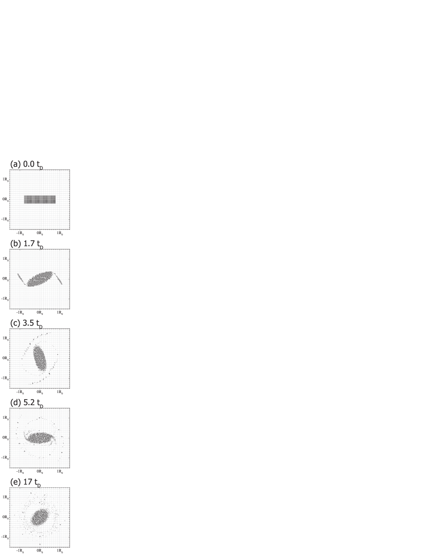
Figure 1: A typical time evolution of the vortices with $\Omega=0.15$, $N=3751$ is shown. Cell size used for the coarse-graining is indicated by the grid lines in gray.

The H function is numerically determined by

$$H(t)=\sum_{i}(\Delta X)^{2}n_{i}(t)\ln n_{i}(t),$$ (87)

with

$$n_{i}(t)=\frac{N_{i}(t)}{(\Delta X)^{2}},\qquad\Delta X=\frac{R_{0}}{10}.$$ (88)

The configuration space is divided into square cells with side $\Delta X$ as is shown by the grid lines in gray in Fig. 1. The number of vortices in the $i$th cell is denoted $N_{i}(t)$. The time evolution of the H function corresponding to Fig. 1 is shown in Fig. 2.

Figure 2: The time evolution of the H function with $\Omega=0.15$, $N=3751$ is shown.

As is predicted by the H theorem, the value of the H function monotonically decreases, which assures that the system settles down to a final equilibrium state characterized by the maximum entropy.

We assume a temporal evolution of the H function as

$$H(t)=H_{0}+H_{1}\exp\left(-\frac{t}{t_{R}}\right).$$ (89)

To determine the relaxation time numerically, simulations with (a) fixed $\Omega$, variable $N$ and (b) fixed $N$, variable $\Omega$ are carried out. The plots of $t_{R}$ versus $1/\Omega$ and $t_{R}/t_{D}$ versus $N$ are shown in Figs. 3 and 4. These plots elucidate the relations $t_{R}\propto 1/\Omega$ and $t_{R}/t_{D}\propto N$.

The scaling $t_{R}/t_{D}\propto N$ for a non-axisymmetric flow agrees with the one previously obtained by Kawahara and Nakanishi Kawahara and Nakanishi (2007). This agreement is interesting because the numerical conditions are different. We work in an unbounded domain and start from a rectangular patch while they work in a bounded domain and start from an annulus. Since our domain is unbounded, no vortex crystal forms. Therefore, the evolution is different but the scaling $t_{R}/t_{D}\propto N$ is the same. Furthermore, we obtain this scaling with a larger number of vortices. Finally, we numerically demonstrate a new scaling law $t_{R}\propto 1/\Omega$ which is predicted by the kinetic equation (68). These numerical results agree with the kinetic theory developed in this paper. It would be nevertheless useful to ascertain these results by making longer simulations and study in more detail the distinction between the collisionless regime (violent relaxation) and the collisional one (slow relaxation). This will be the object of a future paper.

Figure 3: The relaxation time $t_{R}$ is plotted against $\Omega^{-1}$ for fixed $N=3751$. It indicates that $t_{R}$ is proportional to $\Omega^{-1}$.

Figure 4: The relaxation time $t_{R}$ scaled by the dynamical time $t_{D}$ is plotted against $N$ for fixed $\Omega=0.15$. It indicates that $t_{R}/t_{D}$ is proportional to $N$.

VIII Conclusion

We have developed a kinetic theory of point vortices for weak mean flows for which the timescale of the macroscopic motion is long as compared to the decorrelation time. A linear trajectory approximation has been used as a first order approximation to compute the correlation functions appearing in the collision term of the kinetic equation. The smooth vorticity field is the solution of the kinetic equation (68). The results of the kinetic theory agree with the numerical simulations: (i) the H function decreases monotonically ($H$ theorem); (ii) the system relaxes towards the Boltzmann distribution; (iii) the relaxation time scales as $t_{R}\propto 1/\Omega$ and $t_{R}/t_{D}\propto N$. The kinetic theory of point vortices describing “collisions” between point vortices and finite $N$ effects can explain, for example, the destruction of “vortex crystals” that form during the collisionless regime Fine et al. (1995); Kawahara and Nakanishi (2007). Therefore, the kinetic theory developed in the present paper can account for many results of numerical simulations and laboratory experiments. There remains open issues such as the difference of behavior between axisymmetric and non-axisymmetric evolutions that will be considered in future works.

Appendix A Validity of Linear Trajectory Approximation

The validity of the linear trajectory approximation is assessed as follows. There are two important characteristic time scales. One corresponds to the Brownian motion and will be denoted by $\tau_{B}$. The other corresponds to the macroscopic fluid motion and will be denoted by $\tau_{F}$. Using these two characteristic time scales, we will derive a condition where the linear trajectory approximation may be valid.

Consider a microscopic area with both sides $2L$, which is of the same size as the space-averaging area introduced in Sec. V. The box moves with the macroscopic flow velocity. Inside the box, vortices fluctuate due to the Brownian motion. Vortices stay within the same box if the time period is short and the macroscopic orbit of a point vortex may be along the flow. However, if the time period exceeds a certain value, say $\tau_{B}$, vortices leave the box and the macroscopic fluid approximation is no longer valid. The stochastic process due to the Brownian motion is expressed by Eq. (49) and $\tau_{B}$ is estimated by

$$D\tau_{B}=(2L)^{2}.$$ (90)

Within the time scale shorter than $\tau_{B}$, the macroscopic fluid approximation is valid.

On the other hand, the condition that the linear trajectory approximation is valid is equivalent to the time scale where the macroscopic flow orbit is straight. We assume that the macroscopic flow has a circular orbit with a radius of curvature $R_{0}$. As the scale length concerned is macroscopic and longer than $2L$, the Brownian motion cannot be seen. Then the characteristic time scale $\tau_{F}$ which corresponds to the macroscopic fluid motion may be estimated by

$$u\tau_{F}=2\pi R_{0}$$ (91)

which is a turnover time with uniform velocity $u$. In our model, the flow orbit consists of many fragment orbits. Each fragment orbit is approximately obtained by the linear trajectory approximation. The time for a vortex to cross a fragment orbit is less than $\tau_{B}$.

To approximate the integral as shown in Eq. (50), $\nu(t-t_{0})$ must be smaller than 1, namely,

$$\frac{1}{\nu}<t-t_{0}.$$ (92)

By definition, the order of $1/\nu$ is estimated by

$$\frac{1}{\nu}=\frac{2}{k^{2}D}=\frac{2}{D}\frac{(2L)^{2}}{(2\pi)^{2}}=\frac{2}{(2\pi)^{2}}\tau_{B},$$ (93)

where we have used the relation

$$k=\frac{2\pi}{2L}.$$ (94)

¿From Eq. (65), the order of $D$ is estimated by

$$D = \frac{\Omega}{(2\pi)^{3}}\left(\frac{\pi}{L}\right)^{2}\frac{1}{k_{\rm min}}\int\cdots$$ (95)

$$\propto \frac{\Omega}{(2\pi)^{3}}\left(\frac{\pi}{L}\right)^{2}\frac{1}{k_{\rm min}}\frac{N\Omega}{u}$$

$$= \frac{1}{N}\frac{1}{(2\pi)^{3}}\left(\frac{\pi}{L}\right)^{2}\frac{1}{k_{\rm min}}\frac{N\Omega}{u}.$$

The circular flow speed is approximated by its average value as

$$u=R_{0}\omega=R_{0}\frac{N\Omega}{\pi R^{2}}=\frac{N\Omega}{\pi}\frac{R_{0}}{R^{2}}$$ (96)

and

$$\pi R^{2}\omega=N\Omega,$$ (97)

where $R$ is a characteristic length of the system ($R>R_{0}$). Using Eqs. (90), (91), (95), (96), (97) and the relation $k_{\rm min}=2\pi/R$, inequality $\tau_{B}<\tau_{F}$ is rewritten as

$$(2L)^{2}\left(\frac{1}{N}\frac{1}{(2\pi)^{3}}\frac{\pi^{2}}{L^{2}}\frac{R}{2\pi}\frac{N\Omega}{u}\right)^{-1}<\frac{2\pi R_{0}}{u}$$ (98)

or as

$$N<\frac{\pi}{32}\frac{1}{N\Omega}\frac{1}{L^{4}}\frac{R^{5}}{R_{0}}.$$ (99)

Equation (99) gives an upper limit on $N$.

On the other hand, in the usual hydrodynamic picture, there is a lower limit length scale $L_{0}$. A region with size $L_{0}\times L_{0}$ contains only one particle and a larger region with size $L\times L$ contains enough particles and reaches a local thermal equilibrium state. Therefore,

$$L_{0}<L<R.$$ (100)

Then the ratio of the number of the particles is given by

$$\frac{L_{0}^{2}}{\pi R^{2}}=\frac{1}{N}$$ (101)

which implies

$$\frac{1}{N}=\frac{1}{\pi}\frac{L_{0}^{2}}{R^{2}}<\frac{1}{\pi}\frac{L^{2}}{R^{2}}.$$ (102)

Namely, the following relation is obtained:

$$1<\pi\left(\frac{R}{L}\right)^{2}<N.$$ (103)

It is found that there is a lower limit on $N$.

Using Eqs. (99) and (103), we obtain the condition that the linear trajectory approximation is valid:

$$1<\pi\left(\frac{R}{L}\right)^{2}<N<\frac{\pi}{32}\frac{1}{N\Omega}\frac{1}{L^{4}}\frac{R^{5}}{R_{0}}.$$ (104)

If we set $R_{0}=R/2$ and $N\Omega=1$, Eq. (104) is rewritten as

$$1<\pi\left(\frac{R}{L}\right)^{2}<N<\frac{\pi}{16}\left(\frac{R}{L}\right)^{4}.$$ (105)

As we used an $1/N$ expansion to evaluate the collision term, $N$ must be large. But the above evaluation indicates that the value of $N$ has a certain maximum number to validate the linear trajectory approximation. The estimates given above are very approximate but their main goal is to suggest that there is a non-asymptotic regime in which our approach applies.

References

• Newton (2001) P. Newton, The N-Vortex Problem: Analytical Techniques (Springer-Verlag, Berlin, 2001).
• Kraichnan and Montgomery (1980) R. H. Kraichnan and D. Montgomery, Rep. Prog. Phys. 43, 547 (1980).
• Tabeling (2002) P. Tabeling, Phys. Rep. 362, 1 (2002).
• Onsager (1949) L. Onsager, Nuovo Cimento Suppl. 6, 279 (1949).
• Eyink and Sreenivasan (2006) G. L. Eyink and K. R. Sreenivasan, Rev. Mod. Phys. 78, 87 (2006).
• Joyce and Montgomery (1973) G. Joyce and D. Montgomery, J. Plasma Phys. 10, 107 (1973).
• Montgomery and Joyce (1974) D. Montgomery and G. Joyce, Phys. Fluids 17, 1139 (1974).
• Kida (1975) S. Kida, J. Phys. Soc. Jpn. 39, 1395 (1975).
• Kraichnan (1975) R. H. Kraichnan, J. Fluid Mech. 67, 155 (1975).
• Seyler, Jr. (1976) C. E. Seyler, Jr., Phys. Fluids 19, 1336 (1976).
• Pointin and Lundgren (1976) Y. B. Pointin and T. S. Lundgren, Phys. Fluids 19, 1459 (1976).
• Lundgren and Pointin (1977) T. S. Lundgren and Y. B. Pointin, J. Stat. Phys. 17, 323 (1977).
• Ting et al. (1987) A. C. Ting, H. H. Chen,  and Y. C. Lee, Physica 26D, 37 (1987).
• Robert and Sommeria (1991) R. Robert and J. Sommeria, J. Fluid Mech. 229, 291 (1991).
• Eyink and Spohn (1993) G. L. Eyink and H. Spohn, J. Stat. Phys. 70, 833 (1993).
• Bühler (2002) O. Bühler, Phys. Fluids 14, 2139 (2002).
• Yatsuyanagi et al. (2005) Y. Yatsuyanagi, Y. Kiwamoto, H. Tomita, M. M. Sano, T. Yoshida,  and T. Ebisuzaki, Phys. Rev. Lett. 94, 054502 (2005).
• Chavanis (2002) P. H. Chavanis, Statistical mechanics of two-dimensional vortices and stellar systems in Dynamics and thermodynamics of systems with long range interactions, edited by T. Dauxois et al., Lecture Notes in Physics 602, 208 (Springer, 2002)
• Matthaeus et al. (1991) W. H. Matthaeus, W. T. Stribling, D. Martinez, S. Oughton,  and D. Montgomery, Physica D 51, 531 (1991).
• Montgomery et al. (1992) D. Montgomery, X. Shan,  and W. H. Matthaeus, Phys. Fluids A4, 3 (1992).
• Li and Montgomery (1996) S. Li and D. Montgomery, Phys. Lett. A 218, 281 (1996).
• (22) One usually states the problem the other way round. Given the macroscopic Euler equation (2), which is the physical equation coming from fluid mechanics, it can be proven Marchioro and Pulvirenti (1994) that a continuous vorticity field $\omega({\bm{r}},t)$ may be approximated arbitrarily well over a finite time interval by a collection of point vortices with circulation $\Omega\sim 1/N$ as $N\rightarrow+\infty$.
• Chavanis (2001) P. H. Chavanis, Phys. Rev. E 64, 026309 (2001).
• Chavanis (2008) P. H. Chavanis, Physica A 387, 1123 (2008).
• (25) A limitation of this equation is that it neglects some collective effects. In the case of axisymmetric flows, collective effects have been taken into account by Dubin and O’Neil Dubin and O’Neil (1988); Dubin (2003) and Chavanis Chavanis (2012a, b).
• Chavanis and Lemou (2007) P. H. Chavanis and M. Lemou, Eur. Phys. J. B 59, 217 (2007).
• Chavanis (2012a) P. H. Chavanis, J. Stat. Mech. 02, P02019 (2012a).
• Chavanis (2012b) P. H. Chavanis, Physica A 391, 3657 (2012b).
• Chavanis (2010) P. H. Chavanis, J. Stat. Mech. 05, P05019 (2010).
• Heyvaerts (2010) J. Heyvaerts, Month. Not. Royal Astron. Soc. 407, 355 (2010).
• Chavanis (2012c) P. H. Chavanis, Physica A 391, 3680 (2012c).
• Chavanis (2013) P. H. Chavanis, Astron. Astrophys. 556, A93 (2013).
• Kawahara and Nakanishi (2007) R. Kawahara and H. Nakanishi, J. Phys. Soc. Jpn. 76, 074001 (2007).
• Chavanis (1998) P. H. Chavanis, Phys. Rev. E 58, R1199 (1998).
• Dubin (2003) D. H. E. Dubin, Phys. Plasmas 10, 1338 (2003).
• Dubin and O’Neil (1988) D. H. E. Dubin and T. M. O’Neil, Phys. Rev. Lett. 60, 1286 (1988).
• Taylor and McNamara (1971) J. B. Taylor and B. McNamara, Phys. Fluids 14, 1492 (1971).
• Dawson et al. (1971) J. M. Dawson, H. Okuda,  and R. N. Carlile, Phys. Rev. Lett. 27, 491 (1971).
• Okuda and Dawson (1973) H. Okuda and J. M. Dawson, Phys. Fluids 16, 408 (1973).
• (40) For example, this approach could be suitable to analyze the breaking of “vortex crystals” Fine et al. (1995); Kawahara and Nakanishi (2007) due to finite $N$ effects (collisions).
• Klimontovich (1967) Y. L. Klimontovich, The statistical theory of non-equilibrium processes in a plasma (MIT Press, Cambridge, Massachusetts, 1967).
• (42) Actually the form of this collision kernel was “guessed” by one of us (PHC) a long time ago, in order to conserve the energy, before finding that the conservation of energy could also be achieved by the delta function in Eq. (6).
• Fine et al. (1995) K. S. Fine, A. C. Cass, W. G. Flynn,  and C. F. Driscoll, Phys. Rev. Lett. 75, 3277 (1995).
• Not (e) The collisional evolution may also be described by the kinetic equation (6) that approaches the Boltzmann distribution without necessarily reaching it (see the discussion in Chavanis (2010)).
• Marchioro and Pulvirenti (1994) C. Marchioro and M. Pulvirenti, Mathematical Theory of Incompressible Nonviscous Fluids (Springer, New-York, 1994).