Assessment of Cowling approximation in computing ellipticity of a magnetized non-barotropic star

Abstract

A deformation of a neutron star due to its own magnetic field is an important issue in gravitational wave astronomy, since a misaligned rotator with small ellipticity may emit continuous gravitational wave that may be observed by ground-based detectors. Recently Mastrano et al. (Mastrano et al. 2011, 2013) evaluated deformations induced by both poloidal and toroidal magnetic field in non-barotropic model stars by neglecting the gravitational field perturbation (Cowling approximation). Following their treatment in non-barotropic fluid and magnetic configurations, we here assess the effect of gravitational perturbation that they neglected. We show that the ellipticity computed with gravitational perturbation is roughly twice as large as that obtained by Cowling approximation. We should allow this amount of error in using the neat analytic treatment proposed by them.

1 Introduction

A rotating neutron star with a non-axisymmetric deformation with respect to the rotational axis emits gravitational wave because of its time-dependent mass quadrupole. The quadrupole scales as the ellipticity $\epsilon$ of the deformed star (see Eq.(11)). Therefore there is a strong astrophysical motivation to compute how much ellipticity we may expect in neutron stars. One of the possibilities that have been proposed to allow misaligned deformation of rotating neutron stars is the magnetic deformation of the stars. Radio pulsars are regarded as a misaligned rotator with strong magnetic field (with typical surface fields $B\sim 10^{8}$ T ($10^{12}$ Gauss)). We now have another class of neutron stars with super-strong field ($B\geq 10^{9}$ T), i.e.,’magnetars’. Although the magnetic fields outside the stars are usually assumed to be dipolar, the configuration of magnetic field inside the stars is unknown. Chung & Melatos (2011) gives observational evidences of the dipolar field in some of the millisecond pulsars, while there are indications that some of the neutron stars may have multipole magnetic field (see Mastrano et al. (2013)).

The deformation of a neutron star due to magnetic field strongly depends on its internal field configuration and we may have a clue to the internal magnetic configuration when the gravitational waves from misaligned rotators are observed.

The studies on the issue of magnetic deformation of neutron stars have been mainly studied under the assumptions of barotropic stars ( general relativistic studies are found for instance in Bonazzola & Gourgoulhon (1996); Colaiuda et al. (2008); Ciolfi et al. (2010); Newtonian counterparts are found in Tomimura & Eriguchi (2005); Yoshida et al. (2006); Haskell et al. (2008); Lander & Jones (2009); Fujisawa et al. (2012)).

Strictly speaking a neutron star is, however, a non-barotropic star which has a density stratification due to a gradient of chemical composition (Reisenegger & Goldreich 1992; Reisenegger 2009). In this case the restrictions on a possible magnetic field structure inside may be rather relaxed compared to the barotropic stars. This is because the gas pressure $p$ is not restricted by an one-parameter equation of state of density $\rho$ such as $p=p(\rho)$ .

Under this physical picture, Mastrano et al. (2011, 2013) evaluated deformations induced by both poloidal and toroidal magnetic field in non-barotropic model stars. They first prescribe the functional form of magnetic field and compute the density perturbation induced by the Maxwell stress. In these studies the perturbation of gravitational potential is neglected (Cowling approximation). The former studies of deformations of neutron stars with crust suggest that Cowling approximation is According to the stellar perturbation theory (Unno et al. 1989), the perturbed gravitational potential for non-axisymmetric perturbations becomes asymptotically zero with increasing number of azimuthal nodes. For axisymmetric perturbation of a lower order this is not the case, and we may expect a large errors in neglecting gravitational perturbation. It is therefore to important to know how large errors we may have in adopting Cowling approximation to compute a small deformation of a star by magnetic stress.

In this paper we compare the ellipticity of magnetized non-barotropic star with and without gravitational perturbation, by following the formulation in Mastrano et al. (2011, 2013).

2 Formulation

We mainly follow the formulation made by Mastrano et al. (2011), except for the treatment of density perturbation in the presence of magnetic field. Magnetic field is treated as a perturbation to a non-magnetic spherical star with density and pressure stratification. The density profile of the non-magnetic star is prescribed and the pressure profile is adjusted so that it balances the local gravitational acceleration. Here we consider their ”parabolic” density profile $\rho(r)$,

$$\rho=\frac{15M_{\star}}{8\pi R_{\star}^{3}}(1-r^{2}),$$ (1)

where $M_{\star},R_{\star}$ are the stellar mass and radius. The radial coordinate $r$ is normalized by $R_{\star}$. The gravitational potential $\Phi$ consistent with the density profile is

$$\Phi=\frac{GM_{\star}}{2R_{\star}}\left(\frac{5r^{2}}{2}-\frac{3r^{4}}{4}-\frac{15}{4}\right)$$ (2)

and the stratified pressure distribution $p(r)$ balancing with the gravity is

$$p=\frac{15M_{\star}^{2}}{16\pi R_{\star}^{4}}\left(1-\frac{5r^{2}}{2}+2r^{4}-\frac{r^{6}}{2}\right).$$ (3)

Axisymmetric magnetic field is imposed on the non-magnetic star above. The magnetic field $\vec{B}$ is determined by two scalar functions $\alpha$ and $\beta$ as

$$\vec{B}=B_{0}[\eta_{{}_{P}}\nabla\alpha\times\nabla\phi+\eta_{{}_{T}}\beta\nabla\phi],$$ (4)

where $B_{0}$ is a constant and $\beta$ is a functional of $\alpha$. $\eta_{{}_{P}}$ and $\eta_{{}_{T}}$ are parameters determining the poloidal and toroidal magnetic field amplitude. We adopt the analytic profile of $\alpha$ as in Mastrano et al. (2011) and their functional form of $\beta$

$$\alpha=\frac{35}{8}\left(r^{2}-\frac{6r^{4}}{5}+\frac{3r^{6}}{7}\right),$$ (5)

and

$$\beta=\left\{\begin{array}[]{cc}(\alpha-1)^{2}&(\alpha\geq 1)\\ 0&(\alpha<1).\end{array}\right.$$ (6)

Lorentz force by the magnetic field modifies the density and pressure distribution inside the star. The magnetic stress is treated as a small perturbation and we consider the linear perturbation $\delta\rho,\delta p$ and the perturbation of gravitational potential $\delta\Phi$. The force balance including magnetic stress is

$$\frac{1}{\mu_{0}}(\nabla\times\vec{B})\times\vec{B}=\nabla\delta p+\delta\rho\nabla\Phi+\rho\nabla\delta\Phi,$$ (7)

where the last term on the right hand side is neglected in Mastrano et al. (2011). We here adopt SI unit. By integrating $\theta$-component of Eq.(7) we obtain the following relation,

$$\delta p+\rho\delta\Phi = -\frac{B_{0}^{2}\alpha}{\mu_{0}r^{2}\sin^{2}\theta}\left[\eta_{{}_{P}}^{2}\hat{\triangle}\alpha\right.$$ (8)

$$\left.+2\eta_{{}_{T}}^{2}\left(\frac{\alpha^{3}}{3}-\frac{3\alpha^{2}}{2}+3\alpha-\ln\alpha-\frac{11}{6}\right)\right],$$

where the operator $\hat{\triangle}=\frac{\partial{{}^{2}}}{\partial r^{2}}+\frac{\sin\theta}{r^{2}}\frac{\partial}{\partial\theta}\left(\frac{1}{\sin\theta}\frac{\partial}{\partial\theta}\right)$ is introduced. Here we omit a monopole term, as is done in Mastrano et al. (2011), since it amounts to rescaling the spherical background star. Then $r$-component of Eq.(7) is written as,

$$\frac{d\Phi}{dr}\delta\rho-\frac{d\rho}{dr}\delta\Phi = \frac{B_{0}^{2}}{\mu_{0}}\eta_{{}_{P}}^{2}\alpha\frac{\partial}{\partial r}\left(\frac{\hat{\triangle}\alpha}{r^{2}\sin^{2}\theta}\right)$$ (9)

$$+\frac{B_{0}^{2}}{\mu_{0}}\cdot 2\eta_{{}_{T}}^{2}\left(\frac{\alpha^{3}}{3}-\frac{3\alpha^{2}}{2}\right.$$

$$\left.+3\alpha-\ln\alpha-\frac{11}{6}\right)\frac{\partial}{\partial r}\left(\frac{\alpha}{r^{2}\sin^{2}\theta}\right).$$

The right hand side is a fixed function of $r,\theta$ when $\alpha$ and $\beta$ are prescribed. It should be noticed that the terms in (8) and (9) having the factor $\eta_{{}_{T}}^{2}$ vanishes when $\alpha<1$. It ensures that the toroidal component of magnetic field is enclosed in the star and no electric current exists in vacuum outside. When Cowling approximation is adopted as in Mastrano et al. (2011), the second term on the left hand side is neglected and $\delta\rho$ is evaluated analytically. We here retain the term and compare the results with those by Cowling approximation. $\delta\Phi$ in the second term is a functional of $\delta\rho$ and written as

$$\delta\Phi(r,\theta)=4\pi G\int dV^{\prime}~{}\delta\rho(r^{\prime},\theta){\cal G}(r^{\prime},\theta^{\prime}|r,\theta)$$ (10)

by using an appropriate Green’s function ${\cal G}$ for Poisson’s equation. We solve Eq.(9) for $\delta\rho$ on a finite-difference grid point by discretizing the integration.

Ellipticity $\epsilon$ that characterizes the stellar deformation due to magnetic field is defined by

$$\epsilon = \frac{I_{zz}-I_{xx}}{I_{0}}$$ (11)

$$= \pi R_{\star}^{5}I_{0}^{-1}\int_{0}^{1}r^{2}dr\int_{0}^{\pi}\sin\theta d\theta~{}\delta\rho~{}r^{2}(1-3\cos^{2}\theta),$$

where $I_{0}$ is the moment of inertia of the non-magnetic spherical star.

The ratio of magnetic field strength in poloidal and toroidal component is measured by the parameter $\Lambda$ which is defined as the ratio of the magnetic energy of poloidal field to the total magnetic energy (the domain of the integrations also includes the vacuum region around the stars),

$$\Lambda=\frac{\int dV\vec{B}_{p}^{2}}{\int dV\vec{B}^{2}}=\frac{\eta_{{}_{P}}^{2}}{\eta_{{}_{P}}^{2}+q\eta_{{}_{T}}^{2}}.$$ (12)

Here $\vec{B}_{p}$ is the first term of Eq.(4). For the prescribed magnetic field (5) and (6), we have $q=1.95\times 10^{-6}$.

3 Results

We first compare the ellipticity computed with and without gravitational perturbation by fixing other model details as in Mastrano et al. (2011). In Fig.1 we plot the ellipticity $\epsilon$ as a function of $\Lambda$ which measures the relative energy of poloidal magnetic field to the total one. The solid line corresponds to the full perturbation when the perturbation of gravitational potential is taken into account. The dashed line is for Cowling approximation as in Mastrano et al. (2011). For this parabolic density profile, the ellipticity of the full perturbation is nearly twice as large as that of Cowling approximation. The fitting formula of $\epsilon$ is

$$\epsilon=1.3\times 10^{-5}\left(\frac{B_{\rm surface}}{5\times 10^{10}{\rm T}}\right)^{2}\left(\frac{M_{\star}}{1.4M_{\odot}}\right)^{-2}\left(\frac{R_{\star}}{10^{4}{\rm m}}\right)^{4}$$

$$\times\left(1-\frac{0.41}{\Lambda}\right),$$ (13)

where $B_{\rm surface}\equiv\eta_{P}B_{0}$.

We also compute the ellipticity for the polytropic case with index $N=1$ which is studied in Mastrano et al. (2011). Compared to the parabolic case, the density profile of the polytrope corresponds to that of a slightly softer equation of state, which shows more concentration near the origin. Overall the density profile is similar to the parabolic one and we confirm that the relative error in Cowling approximation is almost the same as in the parabolic case. $\epsilon$ for this case is fitted as,

$$\epsilon=1.2\times 10^{-5}\left(\frac{B_{\rm surface}}{5\times 10^{10}{\rm T}}\right)^{2}\left(\frac{M_{\star}}{1.4M_{\odot}}\right)^{-2}\left(\frac{R_{\star}}{10^{4}{\rm m}}\right)^{4}$$

$$\times\left(1-\frac{0.40}{\Lambda}\right).$$ (14)

This is, however, only for these particular choices of density and magnetic profile. To see what happens for a different situation, we adopt an extreme case of density profile. A density profile with off-centred maximum is defined as

$$\rho=\frac{15M_{\star}}{8\pi R_{\star}^{3}}\left(r^{2}-r^{3}\right)$$ (15)

with a corresponding gravitational potential

$$\Phi=\frac{GM_{\star}}{2R_{\star}}\left(\frac{r^{4}}{20}-\frac{r^{6}}{42}-\frac{851}{420}\right).$$ (16)

Although this profile is far from realistic, it gives an example showing that the density profile of the non-magnetic background state is as important to determine $\epsilon$ as the magnetic field distribution. In Fig.3 we plot the ellipticity as a function of $\Lambda$ parameter. The magnetic field distribution is the same as in the parabolic density profile case above. We are here interested in the qualitative behaviour and do not care the size of the ellipticity. The ellipticity in Cowling approximation behaves rather differently from that in full perturbation. For a larger poloidal fraction of magnetic field, the full theory predicts prolate deformation of a star while the Cowling approximation produces an oblately deformed star. As the toroidal fraction is increased ( $\Lambda\to 0$), this tendency is reversed. This extreme case shows that we need to take into account gravitational perturbation to compute securely the ellipticity of a star.

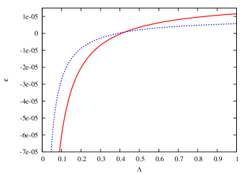
Figure 1: Ellipticity of a stellar model induced by magnetic field (Eq.(4)) is plotted as a function of $\Lambda$ which measures the relative strength of poloidal magnetic field to the total field. The solid line takes into account gravitational perturbation, while the dotted line is for Cowling approximation. The non-magnetic stellar model has a parabolic density profile as Eq.(1). We fix $B_{0}^{2}/(\mu_{0}p_{c})$ to be $10^{-7}$ and $\eta_{P}$ to be unity.

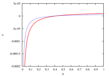
Figure 2: The same as Fig.1 except that the non-magnetic stellar model has a density profile of $N=1$ polytrope.

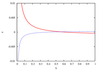
Figure 3: The same as Fig.1 except that the non-magnetic stellar model has an off-centred density maximum.

4 Summary and Comments

Mastrano et al. (2011, 2013) computed the ellipticity induced by the Maxwell stress of density-stratified stars with magnetic field. It is assumed that the deformation is so small that it is treated as a linear perturbation to the non-bartotropic spherical equilibrium. With Cowling approximation in which the Eulerian perturbation of gravitational potential is neglected, they obtain a neat analytic formula for the ellipticity assuming magnetic field to have a prescribed analytic distribution. We assessed the reliability of Cowling approximation in their model by taking the perturbed gravitational potential into account. As is expected from the stellar perturbation theory, Cowling approximation gives rise to a large error in density distribution and the ellipticity depending on the spherical background star as well as on the magnetic distribution. For a comparatively realistic case, however, the deviation of the ellipticity due to Cowling approximation from the actual value may be smaller than an order of magnitude. The result is consistent with the former studies (Ushomirsky et al. 2000; Cutler et al. 2003; Haskell et al. 2006) in which the effects of Cowling approximation on the ellipticity due to crust mountains of neutron stars are estimated. Although the magnetic field instead of the crust shear modulus deforms the stars here, the results obtained are consistent with those in the former studies, i.e., neglecting the gravitational perturbation may suffer a few hundred per cent of errors in the ellipticity for astrophysically relevant models. On the other hand, by comparing the full and the Cowling treatment for non-trivial density distribution we see that neglecting gravitational potential may lead to a rather erroneous result. It may be safe to take into account the gravitational perturbation in computing magnetic deformation of a star.

Finally an extension of the formulations by Tokyo group (Tomimura & Eriguchi 2005; Yoshida et al. 2006; Fujisawa et al. 2012) to include non-barotropic effect may be useful to compute consistently the effect of magnetic field and gravity on the ellipticity of magnetized stars.

References

- Bonazzola & Gourgoulhon (1996) Bonazzola S., Gourgoulhon E., 1996, A&A, 312, 675
- Chung & Melatos (2011) Chung C. T. Y., Melatos A., 2011, MNRAS, 415, 1703
- Ciolfi et al. (2010) Ciolfi R., Ferrari V., Gualtieri L., 2010, MNRAS, 406, 2540
- Colaiuda et al. (2008) Colaiuda A., Ferrari V., Gualtieri L., Pons J. A., 2008, MNRAS, 385, 2080
- Cutler et al. (2003) Cutler C., Ushomirsky G., Link B., 2003, ApJ, 588, 975
- Fujisawa et al. (2012) Fujisawa K., Yoshida S., Eriguchi Y., 2012, MNRAS, 422, 434
- Haskell et al. (2006) Haskell B., Jones D. I., Andersson N., 2006, MNRAS, 373, 1423
- Haskell et al. (2008) Haskell B., Samuelsson L., Glampedakis K., Andersson N., 2008, MNRAS, 385, 531
- Lander & Jones (2009) Lander S. K., Jones D. I., 2009, MNRAS, 395, 2162
- Mastrano et al. (2013) Mastrano A., Lasky P. D., Melatos A., 2013, ArXiv e-prints
- Mastrano et al. (2011) Mastrano A., Melatos A., Reisenegger A., Akgün T., 2011, MNRAS, 417, 2288
- Reisenegger (2009) Reisenegger A., 2009, A&A, 499, 557
- Reisenegger & Goldreich (1992) Reisenegger A., Goldreich P., 1992, ApJ, 395, 240
- Tomimura & Eriguchi (2005) Tomimura Y., Eriguchi Y., 2005, MNRAS, 359, 1117
- Unno et al. (1989) Unno W., Osaki Y., Ando H., Saio H., Shibahashi H., 1989, Nonradial oscillations of stars, University of Tokyo Press, Tokyo
- Ushomirsky et al. (2000) Ushomirsky G., Cutler C., Bildsten L., 2000, MNRAS, 319, 902
- Yoshida et al. (2006) Yoshida S., Yoshida S., Eriguchi Y., 2006, ApJ, 651, 462