Two magnon bound state causes ultrafast thermally induced magnetisation switching

Abstract

There has been much interest recently in the discovery of thermally induced magnetisation switching, where a ferrimagnetic system can be switched deterministically without and applied magnetic field. Experimental results suggest that the reversal occurs due to intrinsic material properties, but so far the microscopic mechanism responsible for reversal has not been identified. Using computational and analytic methods we show that the switching is caused by the excitation of two magnon bound states, the properties of which are dependent on material factors. This discovery allows us to accurately predict the switching behaviour and the identification of this mechanism will allow new classes of materials to be identified or designed to use this switching in memory devices in the THz regime.

Thermally induced ultrafast magnetisation switching (TIMS) is a recent discovery in which an applied sub-picosecond heat pulse causes the magnetic state of a system to switch without any symmetry breaking magnetic field Ostler:2012hx . The lack of any external directional stimulus has long been intriguing and implies the mechanism to be fundamentally intrinsic to the specific class of materials in which it is found. The full microscopic understanding is still lackingMentink:2012ga ; Atxitia:2012vy ; Schellekens:2013wg , and it is not known why switching has only been observed in the ferrimagnets GdFeCoOstler:2012hx and TbCoAlebrand:2012gf . Here we study the phenomenon in GdFeCo using atomistic spin dynamics, supported by analytical calculations based on the linear spin wave theory. We reveal that TIMS results from the strong excitation of two magnon bound states, a hybridisation of ferro- and antiferro-magnetic dynamical modes, relating to specific material dependent conditions. We give detailed quantification of the phenomenon, and thus our study opens pathways for search and design of new classes of materials exhibiting TIMS.

The manipulation of magnetism by using ultrafast external stimuli ($<100$ ps)Stohr:2006wk , such as shaped magnetic field pulses Tudosa:2004jc , acousto-magneto-plasmonics Temnov:2012ve and femtosecond laser pulsesBigot:2009bu ; Kirilyuk:2010vd , is fundamental to future digital data storage technologiesWeller:1999ia . The most promising is the discovery of sub-picosecond magnetisation reversal by TIMS, occurring after the application of a femtosecond laser pulse alone in antiferromagnetically coupled systemsStanciu:2007vh . It opens new avenues for technological developments including proposals for ultrafast, all-optically switched magnetic recording media which will allow a considerable simplification in the design of write transducers and achieve significant energy savings Challener:2009do ; Savoini:2012ik . However, despite extensive experimental deJong:2012kh ; Alebrand:2012il ; Alebrand:2012gf ; Savoini:2012ik ; Khorsand:2012co ; Khorsand:2013cy ; Graves:2013ub and theoretical research Schlickeiser:2012ew ; Mentink:2012ga ; Atxitia:2012vy ; Schellekens:2013wg aimed at revealing the microscopic mechanisms to allow the control of TIMS and the identification of new candidate materials, a satisfactory understanding still does not exist. Shedding new light on the issue is the main subject of this report.

Results

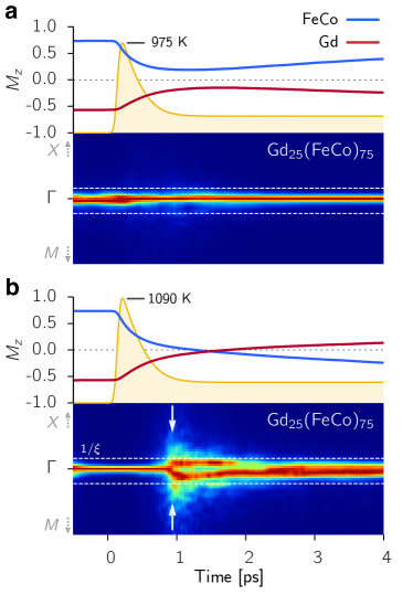
(a)

Figure 1: Intermediate structure factors with laser excitation. Application of a laser pulse to the Gd₂₅(FeCo)₇₅ amorphous lattice model. The blue and red lines are the $M_{z}$ of the FeCo and Gd, normalised to the total magnetisation of each sublattice respectively. The yellow curve shows the thermal energy applied to the system. In the low panels the colour intensity represents the amplitude of magnons at the given $k$-vector in comparison to other vectors at the same instance in time. (a) The laser heating causes a reduction in magnetisation of the two sublattices but the distribution of power in the magnons does not change significantly from the equilibrium distribution. (b) A higher laser fluence causes switching. During the reversal period, magnons on a specific length scale are excited corresponding to the angular momentum transfer channel between AF and FM modes. After reversal the ISF returns to the equilibrium distribution.

To understand the microscopic magnetisation dynamics which lead to TIMS in GdFeCo alloys we first use large-scale atomistic spin dynamics to study time evolution of the spatial Fourier transform of the spin-spin correlation function (the intermediate structure factor - ISF) (see Supplementary Section S2) after the application of a femtosecond laser pulse to observe the distribution of magnons in the Brillouin zone. Figure 1a corresponds to a low laser fluence situation where TIMS is not observed. The ISF shows that the absorbed laser energy ($k_{B}T(t)$) is uniformly distributed within the low wave-vector $k$ modes after the initial heating, leading to a decrease in the magnetisation of both sublattices (upper panel Fig. 1a). After the pulse, the non-equilibrium magnon distribution moves back towards its equilibrium resulting in the gradual recovery in the magnetisation of the sublattices. For a larger laser fluence (Fig. 1b) the initial heating leads to a more pronounced reduction in magnetisation and excitation of a broader $k$-range. While cooling, instead of a relaxation of magnons, one observes an almost instantaneous excitation of magnons within a well defined range in $k$-space. This behaviour is a consequence of magnon-mediated angular momentum transfer between ferromagnetic (FM) and antiferromagnetic (AF) modes through well-defined channels. This initially leads to the so-called transient ferromagnetic-like stateOstler:2012hx which precedes TIMS.

To identify the nature of magnons defining the angular momentum channels, we calculate the dynamic structure factor (DSF), $\mathcal{S}\left({\mathbold{k}},\omega\right)$, to obtain the magnon spectrum (experimentally obtainable via Brillouin experiments). To interpret the ISF in relation to the equilibrium spectrum, one can assume the laser excitation is so fast that only the magnonic population is altered, rather than the spectrum itself. To give a clear contrast of the relative contribution to the spin fluctuations of each magnon branch in the spectrum we perform the normalisation $|\mathcal{S}({\mathbold{k}},\omega)|^{2}/\mathrm{max}(|\mathcal{S}({\mathbold{k}},\omega)|^{2})$ Bergman:2010wb .

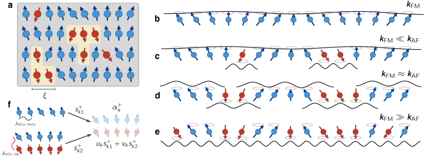
(a)

Figure 2: Effective magnons in amorphous GdFeCo. (a) The lattice is made up of FeCo (blue) and Gd (red) spins. The random distribution of Gd within the lattice forms clusters of connected Gd regions. These have a typical length scale $\xi$ for a given Gd concentration. (b-e) Relevant magnons on different wave-vectors $k$, depend on the Gd content. (b) For a pure FM only FM magnons exist on all wave-vectors $k$. (c) At low Gd concentrations FeCo spin fluctuations are dominated by low $k$ FM magnons, whereas the few Gd spins fluctuate due to the short range AF coupling to the FeCo lattice represented by the dominance of AF magnons at large $k$. (d) At intermediate Gd concentrations ($\sim$ 20-30 %) due to the increase of Gd spins in the system, the AF correlation length characterised by the wave-vector $k_{\mathrm{AF}}$ decreases allowing the existence of AF-FM two magnon bound state spin fluctuations. (e) AF magnons dominate across all length scales. (f) Using linear spin wave theory and the virtual crystal approximation we can represent the system in terms of $\alpha$ and $\beta$ effective magnons which hybridizes the elementary FM and AF modes (see Supplementary Section S4 for details).

The spectrum in ferrimagnetic GdFeCo alloys, (Fig. 2a), contains two kinds of magnons: 1) FM magnons whose low-energy reads $\omega(k)\sim k^{2}$ (see Fig. 2b) and 2) the AF magnons ($\omega\sim k$) which relate mainly to FeCo-Gd spin-fluctuations Haug:1972vm ; Mekonnen:2011dp . The magnon spectrum evolves in a characteristic manner with increasing Gd concentration as shown schematically in figures. 2c-e. At low density, where the Gd can be considered an impurity in the FeCo lattice, the spectrum is dominated mainly by the FeCo spin-fluctuations (Fig. 2c), while at high densities of Gd the AF mode dominates (Fig. 2e). In the intermediate density range (Fig. 2d) both FM and AF magnons coexist and, as we will show, it is this region which is central to the origin of TIMS. In this work we use the virtual crystal approximation (VCA) to make the disordered lattice tractable within linear spin wave theory (LSWT) and calculate the energy and the contribution of the FM and AF magnons to the spin fluctuations of each sublattice (Fig. 2f).

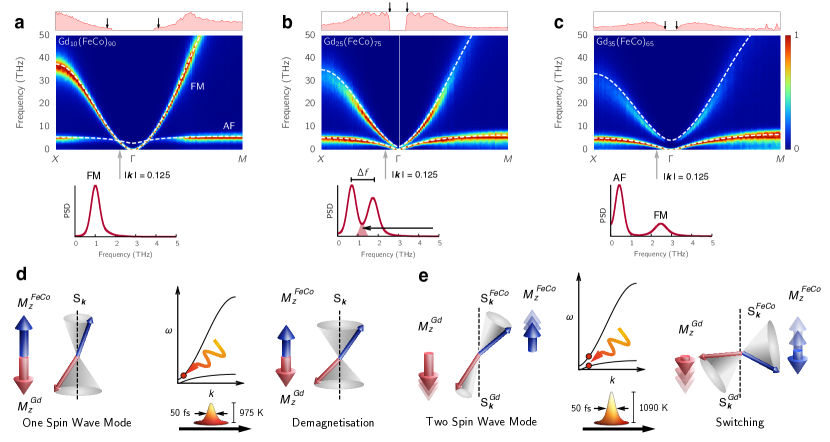
Figure 3: Magnon band structures and explanation of one and two magnon states. (a-c) In each DSF the colour indicates the relative amplitude of magnons modes (the power specturm density). The analytic dispersion from the LSWT is overlaid on each DSF in dashed-white, showing a good agreement with our calculated band structure. The box above each panel gives the amplitude of the two magnon state in red. This is maximised when both bands have the same amplitude and is zero where only one band contains any amplitude. The mean Gd cluster correlation length $\xi$ as calculated from percolation theory is denoted by the black arrows. Below each DSF is a cross section of the power spectrum density (PSD) at the low $k$ vector $|k|=0.125$. (a) Low Gd concentration has distinct FM and AF magnons.The AF band is restricted to the edge of the Brillouin zone (colloring scheme) as there are relatively few, localised FeCo-Gd interactions. The system behaves as a FM due to the dominance of this band. (b) For Gd$\sim$20-30%. there is region near the centre of the Brillouin zone with the two magnon state and a small frequency gap ($\Delta f$) between the two bands. The shaded region in the PSD is where non-linear interactions allow the efficient transfer of angular momentum between sublattices. Strong excitation of these magnons causes TIMS. (c) High Gd concentration reduces the two magnon state and the large frequency gap stops the flow of angular momentum between the FM and AF modes. (d) Excitation of one magnon modes causes a reduction in the magnetisation. (e) Two magnon modes cause localised oscillations in the magnetisation. Strong excitation of these states causes a transfer of angular momentum between FM and AF modes leading to the transient ferromagnetic state and switching.

At low Gd concentration, where TIMS is not observed in our simulations or in experiments Khorsand:2013cy , the distinction between FM and AF magnons is well manifested (Fig 3a). FM magnons are dominant across the Brillouin zone, and it is only at the edge of the Brillouin zone where the few localised FeCo-Gd interactions play a role. This indicates the suppression of AF excitations on longer length scales (small $k$) within the lattice and thus the interaction-induced AF correlation length is range-limited. Therefore, in the low-energy regime GdFeCo essentially behaves as a ferromagnet slightly perturbed by Gd impurities. Spin fluctuations are mixed only at very short interaction length scales (large $k$ values) which are very high in energy, so the laser heating excites only FM modes leading to a reduction in magnetisation (Fig. 3d).

As the Gd concentration increases, so does the FeCo-Gd AF exchange interaction correlation length(Fig. 2d). Consequently in the FeCo lattice the relative FM magnon contribution to spin fluctuations loses amplitude at large length scales in favour of the AF modes (Fig. 3b), gradually diminishing the ferromagnetic character of such spin fluctuations to a FM-AF magnon mixing, the two magnon bound state. For 20-30% Gd, there is a strong interplay between the two bands and a region develops close to the centre of the Brillouin zone where the relative amplitude of both magnon branches is similar, leading to localised oscillations in the magnetisation vector that can be excited by the laser energy as shown in figure 3e. This is a key factor to allow angular momentum transfer between the modes which scales with the intersecting area of the two modes power spectrum (see PSD cross section below Fig. 3b). This area is maximised when gap between the bands, $\Delta f$ is minimised. For TIMS to occur the flow of angular momentum from FM to AF modes must be enhanced which is satisfied by increasing laser fluence because the number of magnons transferring angular momentum is increased.

For even larger Gd content ($>35\%$) FeCo-Gd interactions play the dominant role in the lattice (Fig. 2e). The system takes on the character of an antiferromagnet with little contribution from the FM band (Fig. 3c). The large frequency gap $\Delta f$ means that there is negligible interaction between two magnon modes, reducing angular momentum transfer, so applying laser energy causes the system to demagnetise via one magnon excitations as in figure 3d.

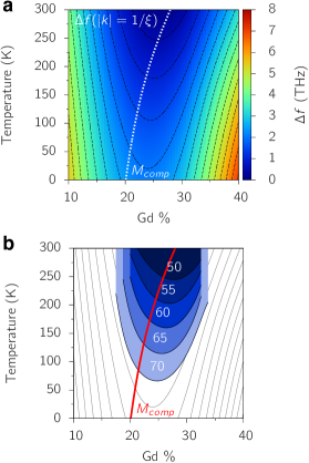
(a)

Figure 4: TIMS reversal windows. (a) The band frequency difference $\Delta f$ at the cluster correlation length $\xi$, calculated from LSWT with VCA and percolation theory. The spacial localisation of the Gd clusters means the minimum does not lie on $M_{comp}$. Smaller $\Delta f$ means that the two magnon modes can more efficiently transfer angular momentum and magnetisation between sublattices when sufficiently excited. (b) TIMS switching windows found from atomistic spin dynamics for different laser fluences. Each enclosed area is the parameter set where switching occurs for the labelled laser fluence. The switching windows closely match the energy contours from diagram (a) (shown in grey).

The minimum laser energy required to initiate switching is essential in the interpretation of experimentsVahaplar:2009fp ; Khorsand:2012co . Laser induced magnetisation switching was first observed to depend on the chirality of the laser pulse Stanciu:2007fy but was later shown using linear lightOstler:2012hx . The threshold energy is helicity dependent because of magnetic circular dichroism Khorsand:2012co . We propose the following criterion for TIMS. First, the frequency gap $\Delta f(k)$ between both magnon branches should be minimised, to maximise the angular momentum transfer through nonlinear interactions (Fig. 3b). Second, the laser energy must be sufficient to strongly excite the $k$-region corresponding to the two magnon bound states. To define this region we use percolation theory to quantify the statistical properties of clusters of Gd on the lattice (Fig. 2a) and find the typical correlation length $\xi$ of clusters (see Methods section). The significance is that $\xi$ directly relates to the length scale of the AF FeCo-Gd interactions. We plot $1/\xi$ as dashed white lines in Fig. 1 where it matches the excited region during switching and as black arrows in the top panels in Fig 3a-c where it matches the extent of the two magnon state in the DSF, shown in red above each panel. From our analytic framework incorporating the LSWT with the VCA and using $\xi$ calculated via percolation theory, we can calculate $\Delta f(1/\xi)$, the frequency difference of the low energy two magnon states, for a range of equilibrium temperatures, $T=0-300$ K and Gd concentrations, $\%=10-40$ (Fig. 4a). To test our premiss that the threshold laser energy to induce TIMS scales with $\Delta f(1/\xi)$ we perform many computational simulations as in Fig. 1 to find the parameter regions where TIMS occurs. Fig. 4b) shows the switching regions for different laser fluences (as labelled). The criterion $\Delta f(1/\xi)$ is smallest around Gd concentrations of $25\%$, but does not exactly follow the magnetisation compensation point, $M_{\mathrm{comp}}$, where the magnetisation of each sublattice is equal. This deviation directly relates to the Gd clustering which limits the range of the two magnon states. In larger samples the FeCo clustering around Gd rich regions can produce the inverse effect, namely, showing a transfer of angular momentum to FeCo clusters with the consequence of Gd region reversing first Graves:2013ub .

Discussion

Our study has identified the nature of TIMS as the magnon-mediated angular momentum transfer between ferromagnetic subsystems with antiferromagnetic coupling between them. Our quantitative analysis opens the door for design of magnetic heterostructures for more energy-efficient all-optical storage devices Stanciu:2007fy , and an enhancement of the information processing rates into the elusive THz regime Kimel:2007fe . The angular momentum transfer channels identified in this work as being essential for the occurrence of TIMS, can be directly accessed by THz radiation Kampfrath:2010kl ; Wienholdt:2012cm . Operation in the THz range leads to a range of benefits as it allows substantially reducing the heat generation that leads to material fatigue and device performance degradation. Additionally, due to the problem with sourcing the rare-earth materials, the large-scale technological impact relies on the discoveries of new cost-friendly TIMS-exhibiting materials. The relatively small parameter space necessary for existence of TIMS in natural materials such as the GdFeCo alloys can be broadened via engineering of heterostructures, for instance, superlattices made of ferromagnetic layers with strong AF coupling, and by improving the inter-lattice magnon-exchange efficiency.

Methods

Lattice Impurity Model

We model the GdFeCo on a simple cubic lattice with Gd moments placed on sites with a uniform random probability. Other sites are considered as an effective FeCo combined moment. The simulations are performed with a Heisenberg like Hamiltonian

$$\mathcal{H}=-\sum_{\langle ij\rangle}J_{ij}^{\mathrm{(}FeCo-FeCo)}{\mathbold{S}}_{i}\cdot{\mathbold{S}}_{j}-\sum_{\langle ij\rangle}J_{ij}^{\mathrm{(}Gd-Gd)}{\mathbold{S}}_{i}\cdot{\mathbold{S}}_{j}-\sum_{\langle ij\rangle}J_{ij}^{\mathrm{(}FeCo-Gd)}{\mathbold{S}}_{i}\cdot{\mathbold{S}}_{j}-\sum_{i}D_{z}S_{z,i}^{2}$$ (1)

The laser heating is modelled using a two-temperature model representing the coupled phonon and electron heat baths. The spin degrees of freedom are coupled to the electronic temperature. Calculation of the dynamic structure factor was by means of a three dimensional spacial discrete Fourier transform (with periodic boundaries) and temporal discrete Fourier transform where a Hamming window is applied. We use a simple cubic lattice of size $128\times 128\times 128$ and integrate the Landau-Lifshitz-Gilbert Langevin equation for over 800ps of simulated time, giving a frequency resolution of 2.5GHz. The resulting power spectra are then convoluted along constant $k$-vector with a Gaussian kernel of width $\sim 0.95$THz and normalised so the largest peak is unity (an example is given in Supplementary Fig. 1).

Linear Spin Wave Theory

We first use the virtual crystal approximation to make the disordered lattice Hamiltonian in Eq. (1) translationally symmetric with respect to spin variables. The spin dynamics is described by the linear Landau-Lifshitz equation of motion, $\mathrm{d}\mathbf{s}_{i}/\mathrm{d}t=\gamma[\mathbf{s}_{i}\times\mathbf{H}_{\mathrm{eff},i}]$, where $\mathbf{H}_{\mathrm{eff},i}=-\partial\mathcal{H}/\partial\mathbf{s}_{i}$. The resulting equations are then transformed in terms of spin raising and lowering operators $s^{\pm}_{i,\mathrm{FeCo}}=s_{i,\mathrm{FeCo}}^{x}\pm s_{i,\mathrm{FeCo}}^{y}$ and $s^{\pm}_{i,\mathrm{Gd}}=s_{i,\mathrm{Gd}}^{x}\pm s_{i,\mathrm{Gd}}^{y}$ which describes the spin fluctuations around equilibrium. The resulting system of two coupled equations is then Fourier transform to describe the spin fluctuations in the reciprocal space and diagonalised by Bogoliubov-like transformation $\mathbf{s}_{\mathbf{k},\mathrm{FeCo}}=u^{+}_{\mathbf{k}}\alpha_{\mathbf{k}}+u^{-}_{\mathbf{k}}\beta^{{\dagger}}_{\mathbf{k}}$. $\mathbf{s}_{\mathbf{k},\mathrm{Gd}}=u^{-}_{\mathbf{k}}\alpha^{{\dagger}}_{\mathbf{k}}+u^{+}_{\mathbf{k}}\beta_{\mathbf{k}}$, where $\alpha_{\mathbf{k}}$ and $\beta_{\mathbf{k}}$ are the eigenstates (magnons) of the system with frequency $\omega_{\alpha}(\mathbf{k})$ and $\omega_{\beta}(\mathbf{k})$ respectively. More detail is given Supplementary Section S4.

Percolation Theory

Percolation theory provides a general mathematical toolbox for quantifying statistical properties of connected geometrical regions of size $s$ which will here refer to $s$ adjacent Gd atom sites. After identifying such Gd clusters within the lattice using the efficient Hoshen-Kopelman algorithmHoshen:1997ga , discounting small clusters ($s<4$) and percolating clusters spanning the computational cell, we calculate the radius of gyration $R_{st}$ of each cluster remaining within the distribution and obtain the correlation length as:

$$\xi^{2}=\frac{2\sum_{s}s^{2}\sum_{t=1}^{n_{s}}R_{st}^{2}}{\sum_{s}s^{2}n_{s}}$$ (2)

The finite size effects are included via the finite size scaling formula for the correlation length

$$\tilde{\xi}=A|p-p_{c}|^{-1/\nu}$$ (3)

where $p_{c}$ is the percolation threshold for bulk lattice and $\nu$ is correlation length universal critical exponents. The values $p_{c}=0.3116004$ and $\nu=0.875$ for site percolation on a simple cubic lattice and the non-universal constant $A=0.776187$ obtained by fitting Eq. 3 to the cluster data evaluated by statistical counts through the lattice. Thus Eq. 3 allows relating the Gd concentration to the associated typical geometrical size of Gd clusters, and correlates well with the predictions of the LSWT discussed in the text.

References

Supplementary Information

S1 - Atomistic Spin Model

The atomistic modelling used to obtain the dynamic structure follows standard techniques in this area. We include a description of the model here for completeness. We use the Landau-Lifshitz-Gilbert equation

$$\frac{\partial{\mathbold{S}}_{i}}{\partial t}=-\frac{\gamma_{i}}{(1+\alpha_{i}^{2})\mu_{i}}\left({\mathbold{S}}_{i}\times{\mathbold{H}}_{i}+\alpha_{i}{\mathbold{S}}_{i}\times{\mathbold{S}}_{i}\times{\mathbold{H}}_{i}\right)$$ (4)

where $\gamma_{i}$ is the gyromagnetic ratio, $\alpha_{i}$ is the Gilbert damping, $\mu_{i}$ is the magnetic moment and ${\mathbold{H}}_{i}$ is the effective field on a spin ${\mathbold{S}}_{i}$. We can include temperature by writing the LLG as a Langevin equation, where the effective field contains a stochastic process ${\mathbold{\xi}}_{i}$

$${\mathbold{H}}_{i}={\mathbold{\xi}}_{i}-\frac{\partial\mathcal{H}}{\partial{\mathbold{S}}_{i}}$$ (5)

the moments of which are defined as

$$\begin{split}\langle\xi_{i}(t)\rangle&=0\\ \langle\xi_{i,a}(t),\xi_{j,b}(t^{\prime})\rangle&=2k_{B}T\alpha_{i}\delta(|t-t^{\prime}|)\delta_{ij}\delta_{ab}\end{split}$$ (6)

where $a$ and $b$ are Cartesian components. The equation of motion is integrated with the Heun scheme using a time step of $dt$=0.1 fs to ensure numerical stability. The material parameters we use in the model are given in table 1.

FeCo-FeCo Exchange Energy	$J_{ij}$	6.920	J$\times{10^{-21}}$
FeCo-Gd Exchange Energy	$J_{ij}$	-2.410	J$\times{10^{-21}}$
Gd-Gd Exchange Energy	$J_{ij}$	2.778	J$\times{10^{-21}}$
FeCo Anisotropy Energy	$d_{z}$	8.072	J$\times{10^{-24}}$
FeCo Moment	$\mu_{\mathrm{s}}$	1.92	$\mu_{\mathrm{B}}$
FeCo Damping	$\alpha$	0.02
FeCo Gyromagnetic Ratio	$\gamma$	1.00	$\gamma_{e}$
Gd Anisotropy Energy	$d_{z}$	8.072	J$\times{10^{-24}}$
Gd Moment	$\mu_{\mathrm{s}}$	7.63	$\mu_{\mathrm{B}}$
Gd Damping	$\alpha$	0.02
Gd Gyromagnetic Ratio	$\gamma$	1.00	$\gamma_{e}$

Table 1: Atomistic material parameters for GdFeCo in the LLG equation.

The amorphous nature of GdFeCo is modelled by using a simple cubic lattice model but with random placements of Gd moments within the lattice to the desired concentration. Using a very large lattice ($128\times 128\times 128$) allows use to finely control the concentration and also gives a good ensemble of clusters.

The thermal effect of the laser is included by use of the two temperature modelChen:2006bo where the spin system is coupled to the electron temperature.

S2 - Structure Factors

The intermediate structure factor (ISF) is calculated from

$$\mathcal{S}({\mathbold{k}},t)=\frac{1}{N}\sum_{{\mathbold{r}},{\mathbold{r}}^{\prime}}{\mathrm{e}^{{\mathrm{i}}{\mathbold{k}}\cdot({\mathbold{r}}-{\mathbold{r}}^{\prime})}}C\left({\mathbold{r}}-{\mathbold{r}}^{\prime},t\right)$$ (7)

where N is the number of spins and the spin-spin correlation function, $C({\mathbold{r}}-{\mathbold{r}}^{\prime},t)=S_{+}({\mathbold{r}},t)S_{-}({\mathbold{r}}^{\prime},t)$.

The dynamic structure factor (DSF) is calculated from

$$\mathcal{S}\left({\mathbold{k}},\omega\right)=\frac{1}{N}\sum_{{\mathbold{r}},{\mathbold{r}}^{\prime}}{\mathrm{e}^{{\mathrm{i}}{\mathbold{k}}\cdot({\mathbold{r}}-{\mathbold{r}}^{\prime})}}\int{\mathrm{e}^{{\mathrm{i}}\omega t}}C\left({\mathbold{r}}-{\mathbold{r}}^{\prime},t\right)\mathrm{d}t$$ (8)

where $N$ is the number of spins, $C({\mathbold{r}}-{\mathbold{r}}^{\prime},t)$ is the spin-spin correlation function

$$C({\mathbold{r}}-{\mathbold{r}}^{\prime},t)=\langle S_{+}({\mathbold{r}},t)S_{-}({\mathbold{r}}^{\prime},0)\rangle$$ (9)

$S_{+}$, $S_{-}$ are the spin raising and lowing operators and $\langle\cdots\rangle$ denotes a thermodynamic average. Numerically the time integral is performed as a discrete Fourier transform in a Hamming window.

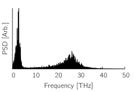
(a) Raw PSD data

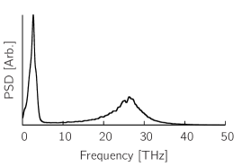
(b) PSD data after Gaussian convolution

Figure 5: The power spectral density along one $k$-vector is filtered using Gaussian convolution with a width of $\sigma=0.95$ THz.

To reduce noise and readability of the structure factors, we apply some data processing. We follow the same techniques used by Bergman et al.Bergman:2010wb . Essentially along each constant $k$-vector, the data is first smoothed with a Gaussian convolution of width  0.95 THz and then normalised so that the maximum value is unity. This means that the mode amplitudes can be compared only on constant $k$-vectors but not between $k$-vectors. This is however, the more useful comparison, especially when looking at the intermediate structure factors. Without normalisation, the large change in temperature across the ISF would make the difference in contrast between low and high temperature too large to reasonably display. Further more we do no wish to compare the absolute value of the amplitude at different times, but rather see which modes are more populated at each given instance in time. An example of the Gaussian convolution is given in figure 5 showing that the data is smoothed but the features remain intact.

S3 - Cluster Counting and Percolation Theory

To identify clusters of Gd sites in the lattice we use the Hoshen-Kopelman methodHoshen:1997ga . This is an efficient algorithm for identifying unique clusters on a lattice. We define a unique cluster as any set of Gd sites which are linked together by a immediate adjacent site (i.e. nearest neighbour exchange coupled). To calculate the typical correlation length, we first remove the tails of the distribution Stauffer:1994uj , that is any cluster of size $s<4$ and the percolating cluster. In practice we discount the single largest cluster to avoid having to calculate if a cluster is percolating. For the calculation of the correlation length, $\xi$ we use the formulaStauffer:1994uj

$$\xi^{2}=\frac{2\sum_{s}s^{2}\sum_{t=1}^{n_{s}}R_{st}^{2}}{\sum_{s}s^{2}n_{s}}$$ (10)

where $s$ is the cluster size, $R$ is the radius of gyration of a cluster and $n_{s}$ is the number of clusters of size $s$. Universal critical exponents are strictly speaking defined only in the thermodynamic limit. Their determination from finite size lattice simulations requires performing the finite size scaling analysisStauffer:1994uj . However, considering very large lattices in our simulations reduces finite size effects and allows direct determination of critical exponents by fitting to the lattices we generate using the form

$$\tilde{\xi}=A|p-p_{c}|^{-\nu}$$ (11)

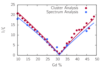
Figure 6: The red points correspond to data taken from cluster analysis using the Hoshen-Kopelman method on the lattice. The blue points are the maximum extent of the two spin wave mode as measured from the Langevin-Landau-Lifshitz-Gilbert dynamic structure factors (see Figure 2 in the main article). The lines correspond to the fit of Eq. (11) where only $A$ is a free parameter. For the cluster analysis $A=0.776187\pm 0.01142$, analysis from the DSF gives $A=0.869468\pm 0.04154$.

where $p_{c}$ is the site percolation threshold which is $0.3116004$ for a simple cubic lattice Grassberger:1992te and the critical exponent $\nu$ is $0.875$ (ref. Lorenz:1998jm, ) and $A$ is the only fitted parameter. The resulting fit is shown in figure 6 along with data extracted directly from the DSF as the maximum length scale of the two-spin region. These show a good agreement as discussed in the article.

S4 - Ferrimagnet Linear Spin Wave Theory

To calculate the LSWT for arbitrary Gd compositions we use the spin analogy of the virtual crystal approximation to transform the disordered lattice Hamiltonian $\mathcal{H}$ describing the system, to a translationally symmetric Hamiltonian $\mathcal{H}_{\mathrm{VCA}}$ with respect to spin variables $\mathbf{S}_{i}$. This involves weighting the material parameters by the relative composition

$$J_{0,\mathrm{11}} =(1-x)zJ_{\mathrm{11}}$$

$$J_{0,\mathrm{22}} =xzJ_{\mathrm{22}}$$

$$J_{0,\mathrm{12}} =xzJ_{\mathrm{12}}$$

$$J_{0,\mathrm{21}} =(1-x)zJ_{\mathrm{21}}$$

where subscripts $1$ and $2$ denote two different species, $x$ is the concentration of species $2$, $z$ is the coordination of the lattice. The spin dynamics is described by the Landau-Lifshitz equation of motion, $\mathrm{d}\mathbf{S}_{i}/\mathrm{d}t=\gamma[\mathbf{S}_{i}\times\mathbf{H}_{\mathrm{eff},i}]$, where $\mathbf{H}_{\mathrm{eff},i}=-\partial\mathcal{H}_{\mathrm{VCA}}/\partial\mathbf{S}_{i}$. The LL equation is then transformed in terms of spin raising and lowering operators $S^{\pm}_{i,\mathrm{FeCo}}=S_{i,\mathrm{FeCo}}^{x}\pm S_{i,\mathrm{FeCo}}^{y}$ which describes the spin fluctuations around equilibrium, in this case the $z-$ axis. The resulting system of two coupled equations is then Fourier transform to describe the spin fluctuations in the reciprocal space

$$\frac{\textrm{d}}{\textrm{d}t}\left(\begin{array}[]{c}s_{\mathbf{k}1}^{+}\\ s_{\mathbf{k}2}^{+}\end{array}\right)=-i\left(\begin{array}[]{cc}\mathcal{A}_{\mathbf{k}11}&\mathcal{B}_{\mathbf{k}12}\\ \mathcal{B}_{\mathbf{k}21}&\mathcal{A}_{\mathbf{k}22}\end{array}\right)\left(\begin{array}[]{c}s_{\mathbf{k}1}^{+}\\ s_{\mathbf{k}2}^{+}\end{array}\right)$$ (12)

where

$$\mathcal{A}_{\mathbf{k}11} =\frac{\gamma}{\mu_{1}}\left(J_{0,11}-J_{\mathbf{k}11}\right)\langle s_{1}\rangle+\frac{\gamma}{\mu_{1}}J_{0,12}\langle s_{2}\rangle$$

$$\mathcal{B}_{\mathbf{k}12} =\frac{\gamma}{\mu_{1}}J_{\mathbf{k}12}\langle s_{2}\rangle$$

$$\mathcal{A}_{\mathbf{k}22} =\frac{\gamma}{\mu_{1}}\left(J_{0,22}-J_{\mathbf{k}22}\right)\langle s_{2}\rangle+\frac{\gamma}{\mu_{1}}J_{0,21}\langle s_{1}\rangle$$

$$\mathcal{B}_{\mathbf{k}21} =\frac{\gamma}{\mu_{2}}J_{\mathbf{k}21}\langle s_{1}.\rangle$$

We include the temperature in a mean field approximation by the self consistent calculation of the values of $\langle s_{1}\rangle$ and $\langle s_{2}\rangle$ Ostler:2011jf . Matrix equation (12) is diagonalised using the Bogoliubov-like transformation $\mathbf{s}_{\mathbf{k},\mathrm{FeCo}}=u^{+}_{\mathbf{k}}\alpha_{\mathbf{k}}+u^{-}_{\mathbf{k}}\beta^{{\dagger}}_{\mathbf{k}}$. $\mathbf{s}_{\mathbf{k},\mathrm{Gd}}=u^{-}_{\mathbf{k}}\alpha^{{\dagger}}_{\mathbf{k}}+u^{+}_{\mathbf{k}}\beta_{\mathbf{k}}$, where $\alpha_{\mathbf{k}}$ and $\beta_{\mathbf{k}}$ are the eigenstates (magnons) of the system with frequency

$$\omega_{\alpha}(\mathbf{k}) =\frac{1}{2}\left[\sqrt{\left(\mathcal{A}_{\mathbf{k}11}+\mathcal{A}_{\mathbf{k}22}\right)^{2}-4\mathcal{B}_{\mathbf{k}12}\mathcal{B}_{\mathbf{k}21}}-\left(\mathcal{A}_{\mathbf{k}22}-\mathcal{A}_{\mathbf{k}11}\right)\right]$$ (13)

$$\omega_{\beta}(\mathbf{k}) =\frac{1}{2}\left[\sqrt{\left(\mathcal{A}_{\mathbf{k}11}+\mathcal{A}_{\mathbf{k}22}\right)^{2}-4\mathcal{B}_{\mathbf{k}12}\mathcal{B}_{\mathbf{k}21}}-\left(\mathcal{A}_{\mathbf{k}11}-\mathcal{A}_{\mathbf{k}22}\right)\right]$$ (14)

where the coefficients of the transformation $u_{\mathbf{k}}$ and $v_{\mathbf{k}}$ read

$$u_{\mathbf{k}} =\sqrt{\frac{1}{2}\left(\frac{\mathcal{A}_{\mathbf{k}11}-\mathcal{A}_{\mathbf{k}22}}{\sqrt{\left(\mathcal{A}_{\mathbf{k}11}+\mathcal{A}_{\mathbf{k}22}\right)^{2}-4\mathcal{B}_{\mathbf{k}12}\mathcal{B}_{\mathbf{k}21}}}+1\right)}$$ (15)

$$v_{\mathbf{k}} =\sqrt{\frac{1}{2}\left(\frac{\mathcal{A}_{\mathbf{k}11}-\mathcal{A}_{\mathbf{k}22}}{\sqrt{\left(\mathcal{A}_{\mathbf{k}11}+\mathcal{A}_{\mathbf{k}22}\right)^{2}-4\mathcal{B}_{\mathbf{k}12}\mathcal{B}_{\mathbf{k}21}}}-1\right)}$$ (16)

Additional Information

Acknowledgements

This work was supported by the EU Seventh Framework Programme under grant agreement No. 281043, FEMTOSPIN. and the Spanish project from Ministry of Science and Innovation under the grant FIS2010-20979-C02-02. U.A. is funded by Basque Country Government under ”Programa Posdoctoral de perfeccionamiento de doctores del DEUI del Gobierno Vasco”. O.H. gratefully acknowledges support from a Marie Curie Intra European Fellowship within the 7th European Community Framework Programme under Grant Agreement No. PIEF-GA-2010- 273014 (MENCOFINAS).

Author Contributions

J.B. and T.O. performed atomistic spin dynamics simulations; J.B., U.A. and O.F. performed the LSWT calculations and interpretation and J.B., O.H. and R.C. carried out the HK cluster analysis and percolation theory. J.B. and U.A. wrote the core of the manuscript, all authors contributed to parts of it.

Competing Financial Interests

The authors declare no competing financial interests.

Figure Legends

References

- (1) Ostler, T. A. et al. Ultrafast heating as a sufficient stimulus for magnetization reversal in a ferrimagnet. Nat. Commun. 3, 666–6 (2012).
- (2) Mentink, J. et al. Ultrafast Spin Dynamics in Multisublattice Magnets. Phys. Rev. Lett. 108, 057202 (2012).
- (3) Atxitia, U. et al. Ultrafast dynamical path for the switching of a ferrimagnet after femtosecond heating. arXiv (2012). eprint 1207.4092v1.
- (4) Schellekens, A. J. & Koopmans, B. Microscopic model for ultrafast magnetization dynamics of multisublattice magnets. Phys. Rev. B (2013).
- (5) Alebrand, S. et al. Light-induced magnetization reversal of high-anisotropy TbCo alloy films. Appl. Phys. Lett. 101, 162408 (2012).
- (6) Stöhr, J. & Siegmann, H. C. Magnetism From Fundamentals to Nanoscale Dynamics (Springer, 2006), 1 edn.
- (7) Tudosa, I. et al. The ultimate speed of magnetic switching in granular recording media. Nature 428, 831–833 (2004).
- (8) Temnov, V. V. Ultrafast acousto-magneto-plasmonics. Nature Photon. (2012).
- (9) Bigot, J.-Y., Vomir, M. & Beaurepaire, E. Coherent ultrafast magnetism induced by femtosecond laser pulses. Nature Physics 5, 515–520 (2009).
- (10) Kirilyuk, A., Kimel, A. V. & Rasing, T. Ultrafast optical manipulation of magnetic order. Reviews of Modern Physics 82, 2731 (2010).
- (11) Weller, D. & Moser, A. Thermal effect limits in ultrahigh-density magnetic recording. IEEE Trans. Magn. 35, 4423–4439 (1999).
- (12) Stanciu, C. D. et al. Subpicosecond magnetization reversal across ferrimagnetic compensation points. Phys. Rev. Lett. 99, 217204 (2007).
- (13) Challener, W. A. et al. Heat-assisted magnetic recording by a near-field transducer with efficient optical energy transfer. Nature Photon. 3, 220–224 (2009).
- (14) Savoini, M. et al. Highly efficient all-optical switching of magnetization in GdFeCo microstructures by interference-enhanced absorption of light. Phys. Rev. B 86, 140404 (2012).
- (15) de Jong, J. et al. Coherent Control of the Route of an Ultrafast Magnetic Phase Transition via Low-Amplitude Spin Precession. Phys. Rev. Lett. 108 (2012).
- (16) Alebrand, S. et al. All-optical magnetization switching using phase shaped ultrashort laser pulses. Phys. Status Solidi A 209, 2589–2595 (2012).
- (17) Khorsand, A. et al. Role of Magnetic Circular Dichroism in All-Optical Magnetic Recording. Phys. Rev. Lett. 108 (2012).
- (18) Khorsand, A. R. et al. Element-Specific Probing of Ultrafast Spin Dynamics in Multisublattice Magnets with Visible Light. Phys. Rev. Lett. 110, 107205 (2013).
- (19) Graves, C. E. et al. Nanoscale spin reversal by nonlocal angular momentum transfer following ultrafast laser excitation in ferrimagnetic GdFeCo. Nature Materials 12, 293–298 (2013).
- (20) Schlickeiser, F. et al. Temperature dependence of the frequencies and effective damping parameters of ferrimagnetic resonance. Phys. Rev. B 86, 214416 (2012).
- (21) Bergman, A. et al. Magnon softening in a ferromagnetic monolayer: a first-principles spin dynamics study. Phys. Rev. B 81, 144416 (2010).
- (22) Haug, A. Magnetic Properties of Solids. In Theoretical Solid State Physics, 282–350 (Pergamon Press, 1972).
- (23) Mekonnen, A. et al. Femtosecond Laser Excitation of Spin Resonances in Amorphous Ferrimagnetic Gd1-xCox Alloys. Phys. Rev. Lett. 107, 117202 (2011).
- (24) Vahaplar, K. et al. Ultrafast Path for Optical Magnetization Reversal via a Strongly Nonequilibrium State. Phys. Rev. Lett. 103, 117201 (2009).
- (25) Stanciu, C. D. et al. All-Optical Magnetic Recording with Circularly Polarized Light. Phys. Rev. Lett. 99, 1–4 (2007).
- (26) Kimel, A. V., Kirilyuk, A. & Rasing, T. Femtosecond opto-magnetism: ultrafast laser manipulation of magnetic materials. Laser & Photon. Rev. 1, 275–287 (2007).
- (27) Kampfrath, T. et al. Coherent terahertz control of antiferromagnetic spin waves. Nature Photon. 5, 31–34 (2010).
- (28) Wienholdt, S., Hinzke, D. & Nowak, U. THz Switching of Antiferromagnets and Ferrimagnets. Phys. Rev. Lett. 108, 247207 (2012).
- (29) Hoshen, J., Berry, M. & Minser, K. Percolation and cluster structure parameters: The enhanced Hoshen-Kopelman algorithm. Phys. Rev. E 56, 1455–1460 (1997).

References

- (1) Chen, J. K., Tzou, D. Y. & Beraun, J. E. A semiclassical two-temperature model for ultrafast laser heating . International Journal of Heat and Mass Transfer 49, 307–316 (2006).
- (2) Bergman, A. et al. Magnon softening in a ferromagnetic monolayer: a first-principles spin dynamics study. Phys. Rev. B 81, 144416 (2010).
- (3) Hoshen, J., Berry, M. & Minser, K. Percolation and cluster structure parameters: The enhanced Hoshen-Kopelman algorithm. Phys. Rev. E 56, 1455–1460 (1997).
- (4) Stauffer, D. & Aharoni, A. Introduction to Percolation Theory (Taylor & Francis, London, 1994), 2 edn.
- (5) Grassberger, P. Numerical studies of critical percolation in three dimensions. J. Phys. A: Math. Gen. 25, 5867 (1992).
- (6) Lorenz, C. & Ziff, R. Precise determination of the bond percolation thresholds and finite-size scaling corrections for the sc, fcc, and bcc lattices. Phys. Rev. E 57, 230–236 (1998).
- (7) Ostler, T. et al. Crystallographically amorphous ferrimagnetic alloys: Comparing a localized atomistic spin model with experiments. Phys. Rev. B 84, 024407 (2011).