A computational framework for
infinite-dimensional Bayesian inverse problems.
Part I: The
linearized case, with application to global seismic
inversion††thanks: This research was partially supported by AFOSR
grant FA9550-09-1-0608; DOE grants DE-FC02-11ER26052,
DE-FG02-09ER25914, DE-FG02-08ER25860, DE-FC52-08NA28615, and DE-SC0009286; and
NSF grants CMS-1028889, OPP-0941678, and DMS-0724746. We are
grateful for this support.
Abstract
We present a computational framework for estimating the uncertainty in the numerical solution of linearized infinite-dimensional statistical inverse problems. We adopt the Bayesian inference formulation: given observational data and their uncertainty, the governing forward problem and its uncertainty, and a prior probability distribution describing uncertainty in the parameter field, find the posterior probability distribution over the parameter field. The prior must be chosen appropriately in order to guarantee well-posedness of the infinite-dimensional inverse problem and facilitate computation of the posterior. Furthermore, straightforward discretizations may not lead to convergent approximations of the infinite-dimensional problem. And finally, solution of the discretized inverse problem via explicit construction of the covariance matrix is prohibitive due to the need to solve the forward problem as many times as there are parameters.
Our computational framework builds on the infinite-dimensional formulation proposed by Stuart [42], and incorporates a number of components aimed at ensuring a convergent discretization of the underlying infinite-dimensional inverse problem. The framework additionally incorporates algorithms for manipulating the prior, constructing a low rank approximation of the data-informed component of the posterior covariance operator, and exploring the posterior that together ensure scalability of the entire framework to very high parameter dimensions. We demonstrate this computational framework on the Bayesian solution of an inverse problem in 3D global seismic wave propagation with hundreds of thousands of parameters.
keywords:
Bayesian inference, infinite-dimensional inverse problems, uncertainty quantification, scalable algorithms, low-rank approximation, seismic wave propagation.AMS:
35Q62, 62F15, 35R30, 35Q93, 65C60, 35L051 Introduction
We present a scalable computational framework for the quantification of uncertainty in large scale inverse problems; that is, we seek to estimate probability densities for uncertain parameters,111We use the term parameters broadly to describe general model inputs that may be subject to uncertainty, which might include model parameters, boundary conditions, initial conditions, sources, geometry, and so on. given noisy observations or measurements and a model that maps parameters to output observables. The forward problem—which, without loss of generality, we take to be governed by PDEs—is usually well-posed (the solution exists, is unique, and is stable to perturbations in inputs), causal (later-time solutions depend only on earlier time solutions), and local (the forward operator includes derivatives that couple nearby solutions in space and time). The inverse problem, on the other hand, reverses this relationship by seeking to estimate uncertain parameters from measurements or observations. The great challenge of solving inverse problems lies in the fact that they are usually ill-posed, non-causal, and non-local: many different sets of parameter values may be consistent with the data, and the inverse operator couples solution values across space and time.
Non-uniqueness stems in part from the sparsity of data and the uncertainty in both measurements and the PDE model itself, and in part from non-convexity of the parameter-to-observable map. The popular approach to obtaining a unique “solution” to the inverse problem is to formulate it as an optimization problem: minimize the misfit between observed and predicted outputs in an appropriate norm while also minimizing a regularization term that penalizes unwanted features of the parameters. Estimation of parameters using the regularization approach to inverse problems as described above will yield an estimate of the “best” parameter values that simultaneously fit the data and minimize the regularization penalty term. However, we are interested not just in point estimates of the best-fit parameters, but a complete statistical description of the parameters values that is consistent with the data. The Bayesian approach [29, 44] does this by reformulating the inverse problem as a problem in statistical inference, incorporating uncertainties in the observations, the parameter-to-observable map, and prior information on the parameters. The solution of this inverse problem is the posterior probability distribution of the parameters, which reflects the degree of confidence in their values. Thus we are able to quantify the resulting uncertainty in the parameters, taking into account uncertainties in the data, model, and prior information.
The inverse problems we target here are characterized by infinite dimensional parameter fields. This presents multiple difficulties, including proper choice of prior to guarantee well-posedness of the infinite-dimensional inverse problem, proper discretization to assure convergence to solutions of the infinite-dimensional problem, and algorithms for constructing and manipulating the posterior covariance matrix that insure scalability to very large parameter dimensions. The approach we adopt in this paper follows [42], which seeks to first fully specify the statistical inverse problem on the infinite-dimensional parameter space. In order to accomplish this goal, we postulate the prior distribution as a Gaussian random field with covariance operator given by the square of the inverse of an elliptic PDE. This choice ensures that samples of the parameter field are (almost surely) continuous as functions, and that the statistical inverse problem is well-posed. To achieve a finite-dimensional approximation to the infinite-dimensional solution, we carefully construct a function-space-aware discretization of the parameter space.
The remaining challenge presented by infinite-dimensional statistical inverse problems is in computing statistics of the (discretized) posterior distribution. This is notoriously challenging for inverse problems governed by expensive-to-solve forward problems and high-dimensional parameter spaces (as in our application to global seismic wave propagation in Section 6). The difficulty stems from the fact that evaluation of the probability of each point in parameter space requires solution of the forward PDE problem (which can take many hours on a large supercomputer), and many such evaluations (millions or more) are required to adequately sample the (discretized) posterior density in high dimensions by conventional Markov-chain Monte Carlo (MCMC) methods. In complementary work [36], we are developing methods that accelerate MCMC sampling of the posterior by employing a local Gaussian approximation of the posterior as a proposal density, which is computed from the Hessian of the negative log posterior. Here, as an alternative, we consider the case of the linearized inverse problem; by linearization we mean that the parameter-to-observable map is linearized about the point that maximizes the posterior, which is known as the maximum a posteriori (MAP) point. With this linearization, the posterior becomes Gaussian, and its mean is given by the MAP point; this can be found by solving an appropriately weighted regularized nonlinear least squares optimization problem. Furthermore, the posterior covariance matrix is given by the Hessian of the negative log posterior evaluated at the MAP point.
Unfortunately, straightforward computation of the—nominally dense—Hessian is prohibitive, requiring as many forward-like solves as there are uncertain parameters (which in our example problem in Section 6, is hundreds of thousands). However, the data are typically informative about a low dimensional subspace of the parameter field: that is, the Hessian of the data misfit term is a compact operator that is sparse with respect to some basis. We exploit this fact to construct a low rank approximation of the (prior preconditioned) data misfit Hessian using matrix-free Lanczos iterations [36, 22], which we observe to require a dimension-independent number of iterations. Each iteration requires a Hessian-vector product, which amounts to just a pair of forward/adjoint PDE solves, as well as a prior covariance operator application. Since we take the prior covariance in the form of the inverse of an elliptic differential operator, its application can be computed scalably via multigrid. The Sherman-Morrison-Woodbury formula is then invoked to express the covariance of the posterior. Finally, we show that the resulting expressions necessary for visualization and interrogation of the posterior distribution require just elliptic PDE solves and vector sums and inner products. In particular, the corresponding dense operators are never formed or stored. Solving the statistical inverse problem thus reduces to solving a fixed number of forward and adjoint PDE problems as well as an elliptic PDE representing the action of the prior. Thus, when the forward PDE problem can be solved in a scalable manner (as it is for our seismic wave propagation example in Section 6), the entire computational framework is scalable with respect to forward problem dimension, uncertain parameter field dimension, and data dimension.
The computational framework presented here is applied to a sequence of realistic large-scale 3D Bayesian inverse problems in global seismology, in which the acoustic wavespeed of an unknown heterogeneous medium is to be inferred from noisy waveforms recorded at sparsely located receivers. Numerical results are presented for several problems with the number of unknown parameters up to 431,000. We have employed a similar approach for problems with more than one million parameters in related work [8].
In the following sections, we provide an overview of the framework for infinite-dimensional Bayesian inverse problems following [42] (Section 2), present a consistent discretization scheme (Section 3) for the infinite-dimensional problem, summarize a method for computing the MAP point (Section 4), describe our low rank-based covariance approximation (Section 5), and present results of the application of our framework to the Bayesian solution of an inverse problem in 3D global seismic wave propagation (Section 6).
2 Bayesian framework for infinite-dimensional inverse problems
2.1 Overview
In the Bayesian formulation, we state the inverse problem as a problem of statistical inference over the space of parameters. The solution of the resulting statistical inverse problem is a posterior probability distribution that reflects our degree of confidence that any set of candidate parameters might contain the actual values that gave rise to the data via the model and were consistent with the prior information. Bayes’ formula, presented in its infinite dimensional form in Section 2.2, defines this posterior probability distribution by combining a prior probability distribution with a likelihood model.
The inversion parameter is a function assumed to be defined over an open, bounded, and sufficiently regular set . The statistical inverse problem is therefore naturally posed in an appropriate function space setting. Here, we adopt the infinite-dimensional framework developed in [42]. In particular, we choose a prior that ensures sufficient regularity of the parameter as required for the statistical inverse problem to be well-posed. We will represent the prior as a Gaussian random field whose covariance operator is the inverse of an elliptic differential operator. For certain problems, non-Gaussian priors can be important, but the use of non-Gaussian priors in statistical inverse problems is still subject to active research, in particular for infinite-dimensional parameters. Thus, here we restrict ourselves to priors given by Gaussian random fields. Let us motivate the choice of the covariance operator as inverse of an elliptic differential operator by considering two alternatives. A common choice for covariance operators in statistical inverse problems with a moderate number of parameters is to specify the covariance function, which gives the covariance of the parameter field between any two points. This necessitates either construction and “inversion” of a dense covariance matrix or expansion in a truncated Karhunen-Loéve (KL) basis. In the large-scale setting, inversion of a dense covariance matrix is clearly intractable, and the truncated KL approach can be impractical since it may require many terms to prevent biasing of the solution toward the strong prior modes. On the contrary, specifying the covariance as the inverse of an elliptic differential operator enables us to build on existing fast solvers for elliptic operators without constructing the dense operator. Discretizations of elliptic operators often satisfy a conditional independence property, which relates them to Gaussian Markov random fields and allows for statistical interpretation [41, 6]. Even if a Gaussian Markov random field is not based on an elliptic differential operator, this Markov property permits the use of fast, sparsity-exploiting algorithms for instance for taking samples from the distribution, [40]. Our implementation employs multigrid as solver for the discretized elliptic systems.
A useful prior distribution must have bounded variance and have meaningful realizations. In our infinite-dimensional setting, we require samples to be pointwise well-defined, for instance, continuous. Furthermore, it is convenient to have the ability to apply the square root of the covariance operator, e.g., this is used to compute samples from a Gaussian distribution. We consider a Gaussian random field on a domain with mean and covariance function describing the covariance between and
| (1) |
The corresponding covariance operator is
| (2) |
for sufficiently regular functions defined over . Thus, if the covariance operator is given by the solution operator of an elliptic PDE, the covariance function is the corresponding Green’s function. Thus, Green’s function properties have direct implications for properties of the random field . For instance, since Green’s functions of the Laplacian in one spatial dimension are bounded, the random field with the Laplacian as covariance operator is of bounded variance. However, in two and three space dimensions, Green’s functions of the Laplacian are singular along the diagonal, and thus the corresponding distribution has unbounded variance. Thus, intuitively the PDE solution operator used as covariance operator has to be sufficiently smoothing and have bounded Green’s functions. Indeed, this is necessary for the well-posedness of the infinite-dimensional Bayesian formulation [42]. The biharmonic operator, for example, has bounded Green’s functions in two and three space dimensions. We choose , where is a Laplacian-like operator specified in Section 2.3. This provides the desired simple and fast-to-apply square root operator and allows a straightforward discretization.
An approach to extract information from the posterior distribution is to find the maximum a posterior (MAP) point, which amounts to the solution of an optimization problem as summarized in Section 2.4. Finally, in Section 2.5, we introduce a linearization of the parameter-to-observable map. This results in a Gaussian approximation of the posterior, which is the main focus of this paper.
2.2 Bayes’ formula in infinite dimensions
To define Bayes’ formula, we require a likelihood function that defines, for a given parameter field , the distribution of observations . Here, we assume a finite-dimensional vector of such observations. We introduce the parameter-to-observable map as a deterministic function mapping a parameter field to so-called observables , which are predictions of the observations. For the problems targeted here, an evaluation of requires a PDE solve followed by the application of an observation operator to extract from the PDE solution. Even when the parameter coincides with the “true” parameter, the observables may still differ from the measurements due to measurement noise and inadequacy (i.e., the lack of fidelity of the governing PDEs with respect to reality) of the parameter-to-observable map . As is common practice, we assume the discrepancy between and to be described by a Gaussian additive noise , independent of . In particular, we have
| (3) |
which allows us to write the likelihood probability density function (pdf) as
| (4) |
The Bayesian solution to the infinite-dimensional inverse problem is then defined as follows: given the likelihood and the prior measure , find the conditional measure of that satisfies the Bayes’ formula
| (5) |
where is a normalization constant. The formula (5) is understood as the Radon-Nikodym derivative of the posterior probability measure with respect to the prior measure . In order for (5) to be well defined, is assumed to be locally Lipschitz and quadratically bounded in the sense of Assumption 2.7 in [42]. While the Bayes’ formula (5) is valid in finite and infinite dimensions, a more intuitive form of Bayes’ formula that uses Lebesgue measures and thus only holds in finite dimensions is given in Section 3.5.
2.3 Parameter space and the prior
As discussed in the introduction of Section 2, we use a squared inverse elliptic operator as covariance operator in (1), i.e., . We first specify the elliptic PDE corresponding to in weak form. For , the solution satisfies
| (6) |
with , and is symmetric, uniformly bounded, and positive definite. Note that for , there exists a unique solution by the Lax-Milgram theorem. Since in (6), regularity results, e.g. [5, 18], show that in fact provided is sufficiently smooth, e.g., is a domain. In this case, satisfies the elliptic differential equation
| (7a) | ||||
| (7b) | ||||
where denotes the outward unit normal on .
Let us denote by the differential operator together with its domain of definition specified by (7); hence is a densely defined operator on with the following domain
The operator is assumed to be “Laplacian-like” in the sense of Assumption 2.9 in [42]. In brief, this assumption requires that be positive definite, self-adjoint, invertible, and have eigenfunctions that form an orthonormal basis of . Additionally, certain growth conditions on the eigenvalues and norms of the eigenfunctions are enforced222We note that this growth condition on the eigenfunctions may not be straightforward to demonstrate (or may not even hold) for a non-rectangular domain and nonconstant coefficient . In these cases, we expect that alternative proofs of the results in [42] can be accessed via regularity properties of the covariance function for the prior distribution. See for example [1, 35]. .
To summarize, we consider as a Gaussian random field whose distribution law is a Gaussian measure on , with mean and covariance operator . The definition of the Gaussian prior measure is meaningful since is a trace class operator on [42], which guarantees bounded variance and almost surely pointwise well-defined samples since holds, where denotes the space of continuous functions defined on (see [42, Lemma 6.25]).
2.4 The MAP point
As a first step in exploring the solution of the statistical inverse problem, we determine the maximum a posteriori (MAP) estimate of the posterior measure. In a finite-dimensional setting, the MAP estimate is the point in parameter space that maximizes the posterior probability density function. This notion does not generalize directly to the infinite-dimensional setting, but we can still define the MAP estimate as the point in parameter space that asymptotically maximizes the measure of a ball with radius centered at , in the limit as . We recall that the Cameron-Martin space equipped with the inner product associated with is the range of [27], and hence coincides with . Using variational arguments, it can be shown (see [42]) that is given by solving the optimization problem
| (8) |
where
| (9) |
The well-posedness of the optimization problem (8) is guaranteed by the assumptions on in Section 2.2.
2.5 A linearized Bayesian formulation
Once we have obtained the MAP estimate , we approximate the parameter-to-observable map by its linearization about , which ultimately results in a Gaussian approximation to the posterior distribution, as shown below. When the parameter-to-observable map is nearly linear this is a reasonable approximation; moreover, there are other scenarios in which the linearization, and the resulting Gaussian approximation, may be useful. Of particular interest here are the limits of small data noise and many observations. In the small noise case, the parameter-to-obvervable map can be nearly linear as a mapping into the subset of the observable space on which the likelihood distribution is non-negligible—even when is significantly nonlinear. The asymptotic normality discussions in [24, 33] suggest that under certain conditions, the many observations case can lead to a Gaussian posterior. Finally, even if this approximation fails to describe the posterior distribution adequately, the linearization is still useful in building an initial step for the rejection sampling approach or a Gaussian proposal distribution for the Metropolis-Hastings algorithm [39, 36]. These methods are related to the sampling algorithm in [25], which also employs derivative information to respect the local structure of the parameter space.
Assuming that the parameter-to-observable map is Fréchet differentiable, we linearize the right hand side of 3 around to obtain
where is the Fréchet derivative of evaluated at . Consequently, the posterior distribution of conditional on is a Gaussian measure with mean and covariance operator defined by [42]:
| (10) |
with denoting the adjoint of , an operator from the space of observations to . In principle, a local Gaussian approximation of the posterior at the MAP point can also be found for non-Gaussian priors and when the noise in the observables is not additive and Gaussian as in (3). In these cases, however, even for a linear parameter-to-observable map the local Gaussian approximation might only be reasonable approximation to the true posterior distribution in a small neighborhood around the MAP point.
3 Discretization of the Bayesian inverse problem
3.1 Overview
Next, we present a numerical discretization of the infinite-dimensional Bayesian statistical inverse problem described in Section 2.2. The discretized parameter space is inherently high-dimensional (with dimension dependent upon the mesh size). If discretization is not performed carefully at each step, it is unlikely that the discrete solutions will converge to the desired infinite-dimensional solution in a meaningful way [42, 32].
In the following, and particularly in Section 3.3, we choose a mass matrix-weighted vector product instead of the standard Euclidean vector product. While this is a natural choice in finite element discretizations [7, 46], this does lead to a few complications, for instance, the use of covariance operators that are not symmetric in the conventional sense (they are self-adjoint however). This choice is much better suited for proper discretization of the infinite-dimensional expressions given in this paper, and the resulting numerical expressions for computation will more closely resemble their infinite-dimensional counterparts in Section 2. By contrast, the correct corresponding expressions in the Euclidean inner product are significantly less intuitive in our opinion, and ultimately more cumbersome to manipulate and interpret than the development we give here.
We provide finite-dimensional approximations of the prior and the posterior distributions in Sections 3.4 and 3.5, respectively. To study and visualize the uncertainty in Gaussian random fields, such as the prior and posterior distributions, we generate realizations (i.e., samples) and compute pointwise variance fields. This must be done carefully in light of the mass-weighted inner products due to the finite element discretization introduced in Section 3.3. We present explicit expressions for computing these quantities for the prior in the Sections 3.6 and 3.7. The fast generation of samples and the pointwise variance field from the Gaussian approximation of the posterior exploits the low rank ideas presented in Section 5. Thus, the presentation of the corresponding expressions is postponed to Section 5.3.
3.2 Finite-dimensional parameter space
We consider a finite-dimensional subspace of originating from a finite element discretization with continuous Lagrange basis functions , which correspond to the nodal points , such that
Instead of statistically inferring parameter functions , we perform this task on the approximation . Consequently, the coefficients are the actual parameters to be inferred. For simplicity of notation, we shall use the boldface symbol to denote the nodal vector of a function in .
3.3 Discrete inner product
Since we postulate the prior Gaussian measure on , the finite-dimensional space inherits the -inner product. Thus, inner products between nodal coefficient vectors must be weighted by a mass matrix to approximate the infinite-dimensional -inner product. We denote this weighted inner product by and assume that is symmetric and positive definite. To distinguish with the -weighted inner product from the usual Euclidean space , we denote it by . For any , observe that , which motivates the choice of as the finite element mass matrix defined by
| (11) |
When using the -inner product, there is a critical distinction that must be made between the matrix adjoint and the matrix transpose. For an operator , we denote the matrix transpose by with entries . The adjoint of , however, must satisfy
| (12) |
This implies that
| (13) |
In the following, we also need the adjoints of and of (for some ), where and are endowed with the Euclidean inner product. The desired adjoints can be can be expressed as
| (14) | ||||
| (15) |
Next, let be the projection from to . Then, the matrix representation for the operator , where and , is implicitly given with respect to the Lagrange basis in by
where is the coordinate vector corresponding to the basis function . As a result, one can write explicitly as
| (16) |
where is given by
3.4 Finite-dimensional approximation of the prior
Next, we derive the finite-dimensional representation of the prior. The matrix representation of the operator defined in Section 2.3 is given by the stiffness matrix with entries
It follows that both and are self-adjoint operators in the sense of (13).
We are now in a position to define the finite-dimensional Gaussian prior measure specified by the following density (with respect to the Lebesgue measure):
| (17) |
This definition implies that .
3.5 Finite-dimensional approximation of the posterior
In infinite dimensions, the Bayes’ formula (5) has to be expressed in terms of the Radon–Nikodym derivative since the prior and posterior distributions do not have density functions with respect to the Lebesgue measure. Since we approximate the prior measure by , it is natural to define a finite-dimensional approximation of the posterior measure such that
where , and is the likelihood (4) evaluated at . If we define as the density of , again with respect to the Lebesgue measure, we recover the familiar finite-dimensional Bayes’ formula
| (18) |
where the normalization constant , which does not depend on , is omitted. Finally, we can express the posterior pdf explicitly as
| (19) |
where, to recall our notation, and . We observe that the negative log of the right side of (19) is the finite-dimensional approximation of the objective functional in (8).
As a finite-dimensional counterpart of Section 2.5, we linearize the parameter-to-observable map at the MAP point, but now considering it as a function of the coefficient vector . Let be the posterior covariance matrix in the -inner product. Using (10), we obtain
| (20) |
with as defined in (14). Note that is self-adjoint, i.e., in the sense of (13).
Since the posterior covariance matrix is typically dense, we wish to avoid explicitly storing it, especially when the parameter dimension is large. Even if we are able to do so, it is prohibitively expensive to construct. The reason is that the Jacobian of the parameter-to-observable map, , is generally a dense matrix, and its construction typically requires forward PDE solves. This is clearly intractable when is large and solving the PDEs is expensive. However, one can exploit the structure of the inverse problem, to approximate the posterior covariance matrix with desired accuracy, as we shall show in Section 5.
3.6 Sample generation in a finite element discretization
We begin by developing expressions for a general Gaussian distribution with mean and covariance matrix . Then, they are specified for the Gaussian prior with . Realizations of a finite-dimensional Gaussian random variable with mean and covariance matrix can be found by choosing a vector containing independent and identically distributed (i.i.d.) standard normal random values and computing
| (21) |
where is a linear map from to such that , in which the adjoint (see also (15)). Note that is a sample from in the mass-weighted inner product.
3.7 The pointwise variance field in a finite element discretization
Let us approximate the covariance function in for a generic Gaussian measure with covariance operator . Recall from Section 2.3 that the covariance function corresponding to the covariance operator is the Green’s function of , i.e.,
where denotes the Dirac delta function concentrated at . We approximate in the finite element space by with coefficient vector . Using the Galerkin finite element method to obtain a finite element approximation of the preceding equation results in
and the entries of the matrix are given by . It follows that and
Let us denote by the representation of in ; then, using (16) yields that Consequently, the discretized covariance function for the covariance operator now becomes
| (22) |
Let us now apply (22) to compute the prior variance field. As discussed in Section 3.4, . This results in the discretized prior covariance function
By taking , the prior variance field at an arbitrary point reads
The pointwise variance field of the posterior distribution builds on the low-rank representation introduced in Section 5. The resulting expression, which requires the prior variance field, is given in (29).
4 Finding the MAP point
Section 2.4 introduced the idea of the MAP point as a first step in exploring the solution of the statistical inverse problem. To find the MAP point, one needs to solve a discrete approximation (using the discretizations of Section 3) of the optimization problem (8), which amounts to a large-scale nonlinear least squares numerical optimization problem. In this section, we provide just a brief summary of a scalable method we use for solving this problem, and refer the reader to our earlier work for details, in particular the work on inverse wave propagation [2, 3, 17]. We use an inexact matrix-free Newton-conjugate gradient (CG) method in which only Hessian-vector products are required. These Hessian-vector products are computed by solving a linearized forward-like and an adjoint-like PDE problems, and thus the Hessian matrix is never constructed explicitly. Inner CG iterations are terminated prematurely when sufficient reduction is made in the norm of the gradient, or when a direction of negative curvature is encountered. The prior operator is used to precondition the CG iterations. Globalization is through an Armijo backtracking line search.
Because the major components of the method can be expressed as solving PDE-like systems, the method inherits the scalability (with respect to problem dimension) of the forward PDE solve. The remaining ingredient for overall scalability is that the optimization algorithm itself be scalable with increasing problem size. This is indeed the case: for a wide class of nonlinear inverse problems, the outer Newton iterations and the inner CG iterations are independent of the mesh size, as is found to be the case for instance for inverse wave propagation [3, 17]. This is a consequence of the use of a Newton solver, of the compactness of the Hessian of the data misfit term (i.e., the first term) in (9), and of the use of preconditioning by , so that the resulting preconditioned Hessian is a compact perturbation of the identity, for which CG exhibits mesh-independent iterations.
5 Low rank approximation of the Hessian matrix
5.1 Overview
As discussed in Section 2.5, linearizing the parameter-to-observable map results in the posterior covariance matrix being given by the inverse of the Hessian of the negative log posterior. Explicitly computing this Hessian matrix requires a (linearized) forward PDE problem for each of its columns, and thus as many (linearized) forward PDE solves are required as there are parameters. For inverse problems in which one seeks to infer an unknown parameter field, discretization results in a very large number of parameters; explicitly computing the Hessian—and hence the covariance matrix—is thus out of the question. As a remedy, we exploit the structure of the problem to find an approximation of the Hessian that can be constructed and dealt with efficiently.
When the linearized parameter-to-observable map is used in (as defined in (9)) and second derivatives of the resulting functional are computed, one obtains the Gauss-Newton portion of the Hessian of . Both, the full Hessian matrix as well as its Gauss Newton portion are positive definite at the MAP point and they only differ in terms that involve the adjoint variable. Since the adjoint system is driven only by the data misfit (see, for instance, the adjoint wave equation 36), the adjoint variable is expected to be small when the data misfit is small, which occurs provided the model and observational errors are not too large. The Gauss-Newton portion of the Hessian is thus often a good approximation of the full Hessian of .
For conciseness and convenience of the notation, we focus on computing a low rank approximation of the Gauss-Newton portion of the (misfit) Hessian in Section 5.2. The same approach also applies to the computation of a low rank approximation of the full Hessian, whose inverse might be a better approximation for the covariance matrix if the data is very noisy and the data misfit at the MAP point cannot be neglected. The low rank construction of the misfit Hessian is based on the Lanczos method and thus only requires Hessian-vector products. Using the Sherman-Morrison-Woodbury formula, this approximation translates into an approximation of the posterior covariance matrix.
5.2 Low rank covariance approximation
For many ill-posed inverse problems, the Gauss-Newton portion of the Hessian matrix (called the Gauss-Newton Hessian for short) of the data misfit term in (9) evaluated at any ,
| (23) |
behaves like (the discretization of) a compact operator (see, e.g., [45, p.17]). The intuitive reason for this is that only parameter modes that strongly influence the observations through the linearized parameter-to-observable map will be present in the dominant spectrum of the Hessian (23). For typical inverse problems, observations are sparse, and hence the dimension of the observable space is much smaller than that of the parameter space. Furthermore, highly oscillatory perturbations in the parameter field often have negligible effect on the output of the parameter-to-observable map. In [10, 11], we have shown that the Gauss-Newton Hessian of the data misfit is a compact operator, and that for smooth media its eigenvalues decay exponentially to zero. Thus, the range space of the Gauss-Newton Hessian is effectively finite-dimensional even before discretization, i.e., it is independent of the mesh. We can exploit the compact nature of the data misfit Hessian to construct scalable algorithms for approximating the inverse of the Hessian [22, 36].
A simple manipulation of (20) yields the following expression for the posterior covariance matrix, which will prove convenient for our purposes:
| (24) |
We now present a fast method for approximating with controllable accuracy by making a low rank approximation of the so-called prior-preconditioned Hessian of the data misfit, namely,
| (25) |
Let be the eigenpairs of , and . Define such that its columns are the eigenvectors of . Replacing by its spectral decomposition (recall that is the adjoint of as defined in (15)),
When the eigenvalues of decay rapidly we can construct a low-rank approximation of by computing only the largest eigenvalues, i.e.,
where contains eigenvectors of corresponding to the largest eigenvalues , and . We can then invert the approximate Hessian using the Sherman-Morrison-Woodbury formula to obtain
| (26) |
where . Equation (26) shows the truncation error due to the low-rank approximation based on the first eigenvalues. To obtain an accurate approximation of , only eigenvectors corresponding to eigenvalues that are small compared to can be neglected. With such a low-rank approximation, the final expression for the approximate posterior covariance is given by
| (27) |
Note that (27) expresses the posterior uncertainty (in terms of the covariance matrix) as the prior uncertainty less any information gained from the data. Due to the square root of the prior in the rightmost term in (27), the information gained from the data is filtered through the prior, i.e., only information consistent with the prior can reduce the posterior uncertainty.
5.3 Fast generation of samples and the pointwise variance field
Properties of the last term in (27), such as its diagonal (which provides the reduction in variance due to the knowledge acquired from the data) can be obtained numerically through just applications of the square root of the prior covariance matrix to columns of . Let us define
then (27) becomes
| (28) |
with .
The linearized posterior is a Gaussian distribution with known mean, namely the MAP point, and low rank-based covariance (28). Thus, the pointwise variance field and samples can be generated as in Section 3.7 and 3.6, respectively. The variance field can be computed as
| (29) |
where , with denoting the th column of , is the function in corresponding to the nodal vector .
Now, we can compute samples from the posterior provided that we have a factorization . One possibility for (see the Appendix for the detailed derivation) reads
| (30) |
with , as a linear map from to , and as the identity map in both and . As discussed in Section 3.6, samples can be then computed as
| (31) |
where is an i.i.d. standard normal random vector.
5.4 Scalability
We now discuss the scalability of the above low rank construction of the posterior covariance matrix in (27). The dominant task is the computation of the dominant spectrum of the prior preconditioned Hessian of the data misfit, , given by (25). Computing the spectrum by a matrix-free eigensolver such as Lanczos means that we need only form actions of with a vector. As argued at the end of Section 3.5, the linearized parameter-to-observable map is too costly to be constructed explicitly since it requires linearized forward PDE solves. However, its action on a vector can be computed by solving a single linearized forward PDE (which we term the incremental forward problem), regardless of the number of parameters and observations . Similarly, the action of on a vector can be found by solving a single linearized adjoint PDE (which we term the incremental adjoint problem). Explicit expressions for the incremental forward and incremental adjoint PDEs in the context of inverse acoustic wave propagation will be given in Section 6. Solvers for the incremental forward and adjoint problems of course inherit the scalability of the forward PDE solver. The other major cost in computing the action of on a vector is the application of the square root of the prior, , to a vector. As discussed in Section 2.3, this amounts to solving a Laplacian-like problem. Using a scalable elliptic solver such as multigrid renders this component scalable as well. Therefore, the scalability of the application of to a vector—which is the basic operation of a matrix-free eigenvalue solver such as Lanczos—is assured, and the cost is independent of the parameter dimension.
The remaining requirement for independence of parameter dimension in the construction of the low rank-based representation of the posterior covariance in (27) is that the number of dominant eigenvalues of be independent of the dimension of the discretized parameter. This is the case when and in (23) are discretizations of a compact and a continuous operator, respectively. The continuity of is a direct consequence of the prior Gaussian measure ; in fact, , the infinite-dimensional counterpart of , is also a compact operator. Compactness of the data misfit Hessian for inverse wave propagation problems has long been observed (e.g., [15]) and, as mentioned above, has been proved for frequency-domain acoustic inverse scattering for both continuous and pointwise observation operators [11, 10]. Specifically, we have shown that the data misfit Hessian is a compact operator at any point in the parameter domain. We also quantify the decay of the data misfit Hessian eigenvalues in terms of the smoothness of the medium, i.e., the smoother it is the faster the decay rate. For an analytic target medium, the rate can be shown to be exponential. That is, the data misfit Hessian can be approximated well with a small number of its dominant eigenvectors and eigenvalues.
As a result, the number of Lanczos iterations required to obtain a low rank approximation of is independent of the dimension of the discretized parameter field. Once the low-rank approximation of is constructed, no additional forward or adjoint PDE solves are required. Any action of in (27) on a vector (which is required to generate samples from the posterior distribution and to compute the diagonal of the covariance) is now dominated by the action of on a vector. But as discussed above, this amounts to an elliptic solve and can be readily carried out in a scalable manner. Since is independent of the dimension of the discretized parameter field, estimating the posterior covariance matrix requires a constant number of forward/adjoint PDE solves, independent of the number of parameters, observations, and state variables. Moreover, since the dominant cost is that of solving forward and adjoint PDEs as well as elliptic problems representing the prior, scalability of the overall uncertainty quantification method follows when the forward and adjoint PDE solvers are scalable.
6 Application to global seismic statistical inversion
In this section, we apply the computational framework developed in the previous sections to the statistical inverse problem of global seismic inversion, in which we seek to reconstruct the heterogeneous compressional (acoustic) wave speed from observed seismograms, i.e., seismic waveforms recorded at points on earth’s surface. With the rapid advances in observational capabilities, exponential growth in supercomputing, and maturation of forward seismic wave propagation solvers, there is great interest in solving the global seismic inverse problem governed by the full acoustic or elastic wave equations [19, 37]. Already, successful deterministic inversions have been carried out at regional scales; for example, see [43, 20, 21, 48, 34].
We consider global seismic model problems in which the seismic source is taken as a simple point source. Sections 6.1 and 6.2 define the prior mean and covariance operator for the wave speed and its discretization. Section 6.3 presents the parameter-to-observable map (which involves solution of the acoustic wave equation) and the likelihood model. We next provide the expressions for the gradient and application of the Hessian of the negative log-likelihood in Section 6.4. Then, we discuss the discretization of the forward and adjoint wave equations and implementation details in Section 6.5. Section 6.6 provides the inverse problem setup, while numerical results and discussion are provided in Sections 6.7 and 6.8.
6.1 Parameter space for seismic inversion
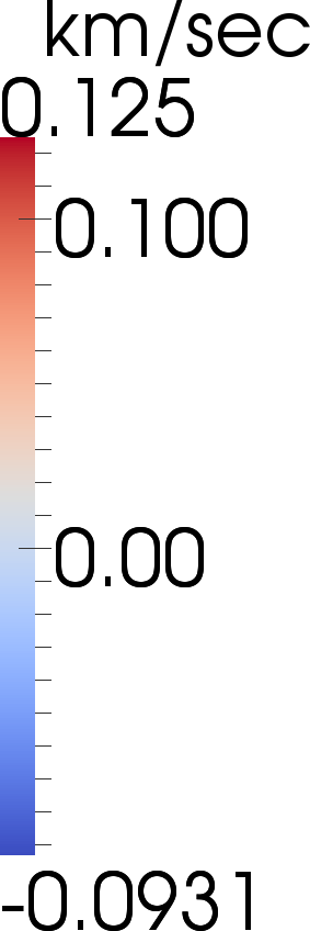
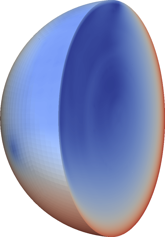
We are interested in inferring the heterogenous compressional acoustic wavespeed in the earth. In order to do this, we represent the earth as a sphere of radius 6,371km. We employ two earth models, i.e.,̇ two representations of the compressional wave speed and density in the earth. We suppose that our current knowledge of the earth is given by the spherically symmetric Preliminary Reference Earth Model (PREM) [16], which is depicted in Figure 1.
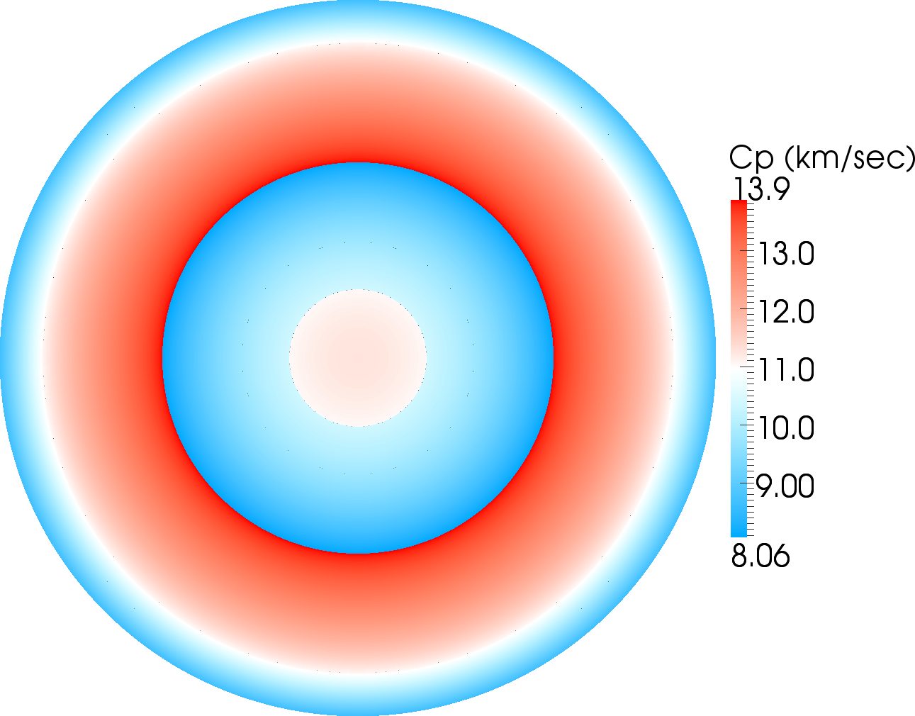
The PREM is used as the mean of the prior distribution, and as the starting point for the determination of the MAP point by the optimization solver. Then, we presume that the real earth behaves according to the S20RTS velocity model [38], which superposes lateral wave speed variations on the laterally-homogeneous PREM. S20RTS is used to generate waveforms used as synthetic observational data for inversion; we refer to it as the “ground truth” earth model. The inverse problem then aims to reconstruct the S20RTS ground truth model from the (noisy) synthetic data and from prior knowledge of the PREM, and quantify the uncertainty in doing so.
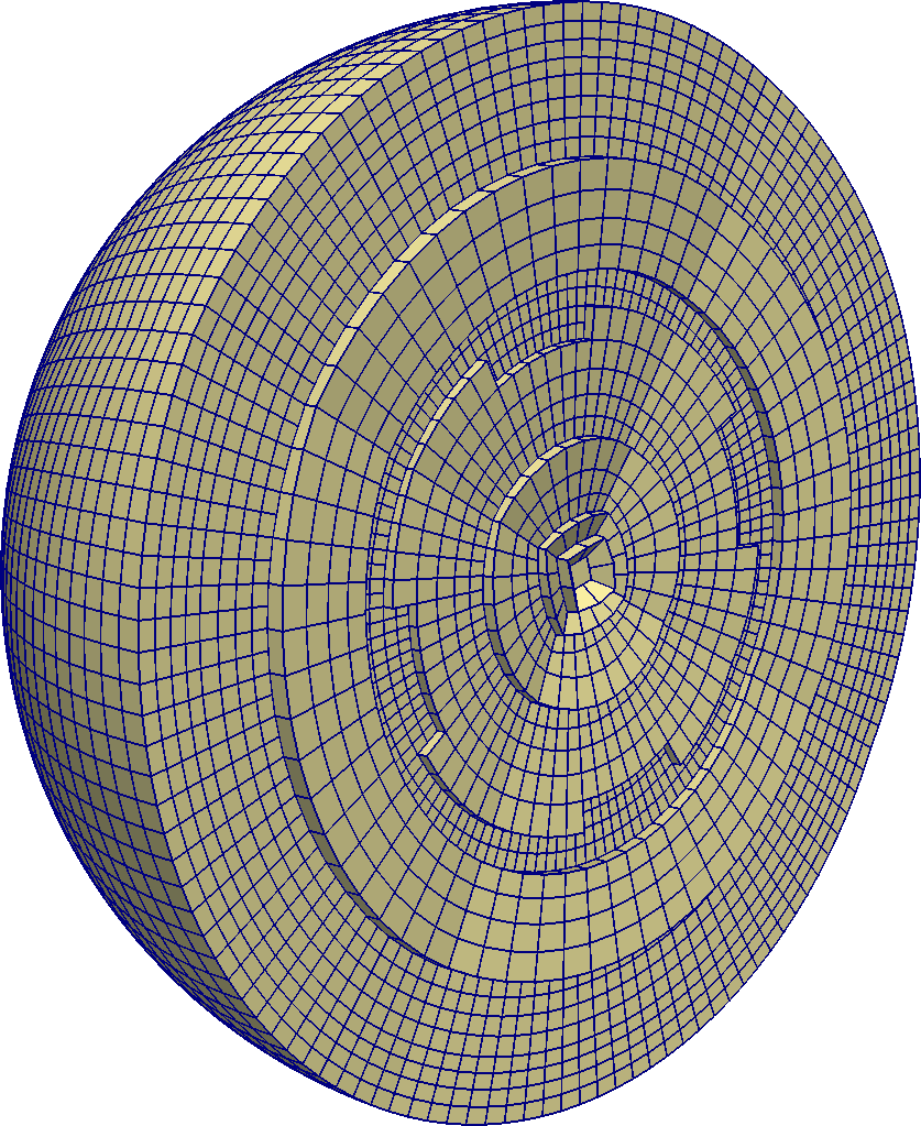
The parameter field of interest for the inverse problem is the deviation or anomaly from the PREM, and hence it is sensible to choose the zero funtion as the prior mean. Owing to the prior covariance operator specified in Section 2.3, the deviation is smooth; in fact it is continuous almost surely. The wave speed parameter space is discretized using continuous isoparametric trilinear finite elements on a hexahedral octree-based mesh. To generate the mesh, we partition the earth into 3 layers described by 13 mapped cubes. The first layer consists of a single cube surrounded by two layers of six mapped cubes. The resulting mesh is aligned with the interface between the outer core and the mantle, where the wave speed has a significant discontinuity (see Figure 1). It is also aligned with several known weaker discontinuities between layers.
The parameter mesh coincides with the mesh used to solve the wave equation described in Section 6.3. The mesh is locally refined to resolve the local seismic wavelength resulting from a given frequency of interest for the PREM. We choose a conservative number of grid points per wavelength to permit the same mesh to be used for anticipated variations in the earth model across the iterations needed to determine the MAP point. For the parallel mesh generation and its distributed storage, we use fast forest-of-octree algorithms for scalable adaptive mesh refinement from the p4est library [13, 12].
6.2 The choice of prior
Since the prior is a Gaussian measure, it is completely specified by a mean function and a covariance operator. As discussed in Section 6.1, the prior distribution for the anomaly (the deviation of the acoustic wavespeed from that described by the PREM model) is naturally chosen to have zero mean. The choice of covariance operator for the prior distribution has to encode several important features. Recall that we specify the covariance operator via the precision operator in Section 2.3. Therefore, the size of the variance about the zero mean is set by , while the product determines the correlation length of the prior Gaussian random field. We next specify the scalar and the tensor based on the following observations of models for the local wave speeds in the earth.
-
•
Smoothness. The parameter field describes the effective local wave-speed, which, for a finite source frequency, depends on the local average of material parameters within a neighborhood of each point in space. This makes the effective wave speed mostly a smooth field. Note that the S20RTS-based target wave speed model (see [38]) is smooth.
-
•
Prior variance. The deviation in this effective wave speed from the PREM model is believed to be within a few percent. Thus, we select such that the prior standard deviation is about 3.5%. The S20RTS target model has a maximal deviation from PREM of 7%.
-
•
Anisotropy in the mantle. We further incorporate the prior belief that the compressional wave speed has a stronger variation in depth than in the lateral directions. We encode this anisotropic variation through . In particular, we select such that the anisotropy is strongest near the surface, and gradually becomes weaker with higher overall correlation length at larger depths. We observe that the S20RTS target model also obeys a similar anisotropy.
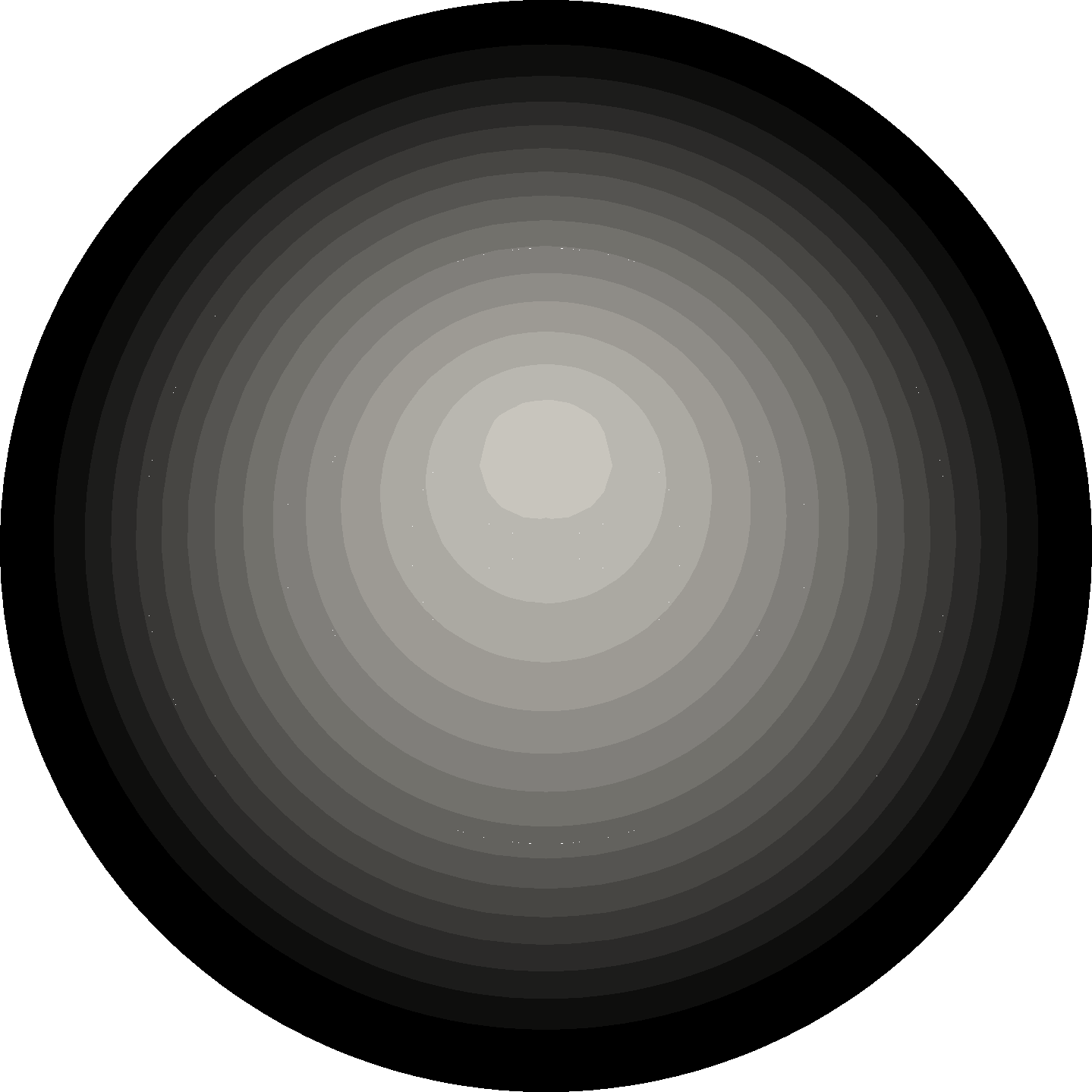
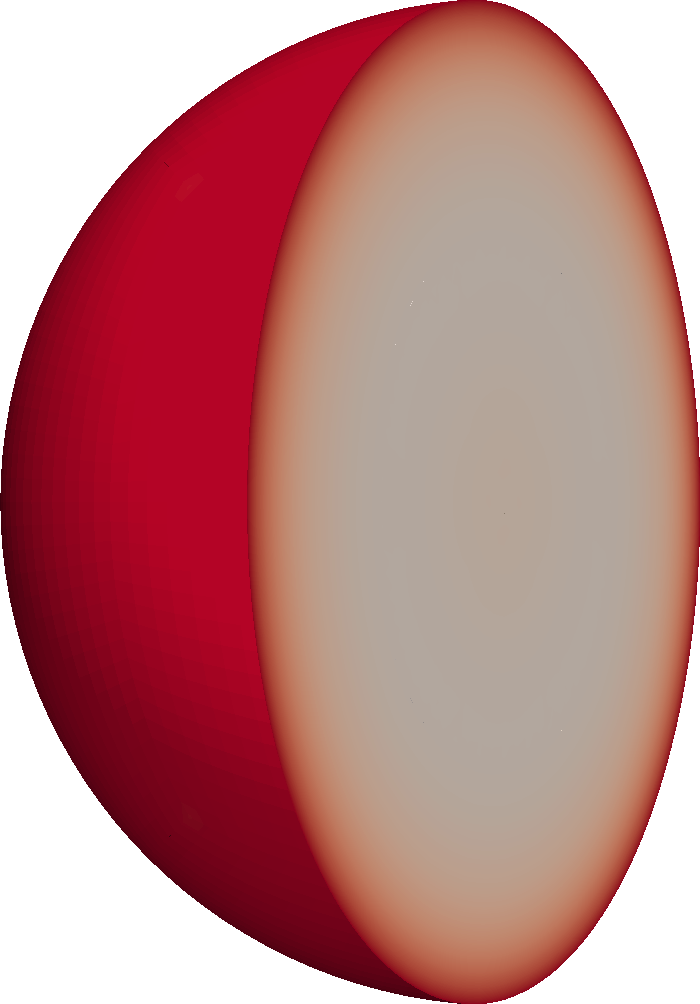
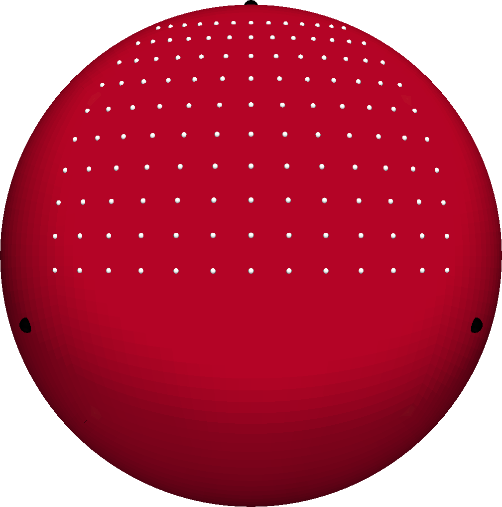
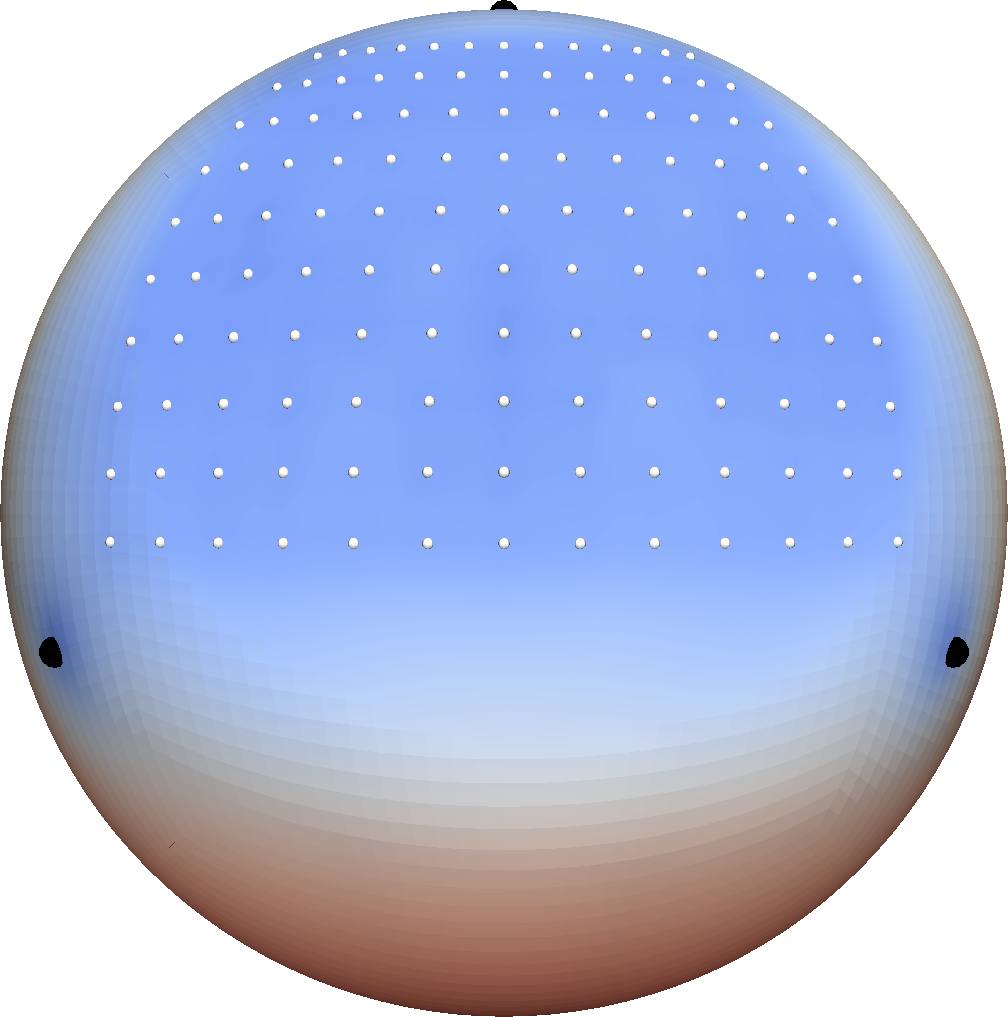
From the preceding observations and discussion, we choose , while is chosen to have the following form
| (32) |
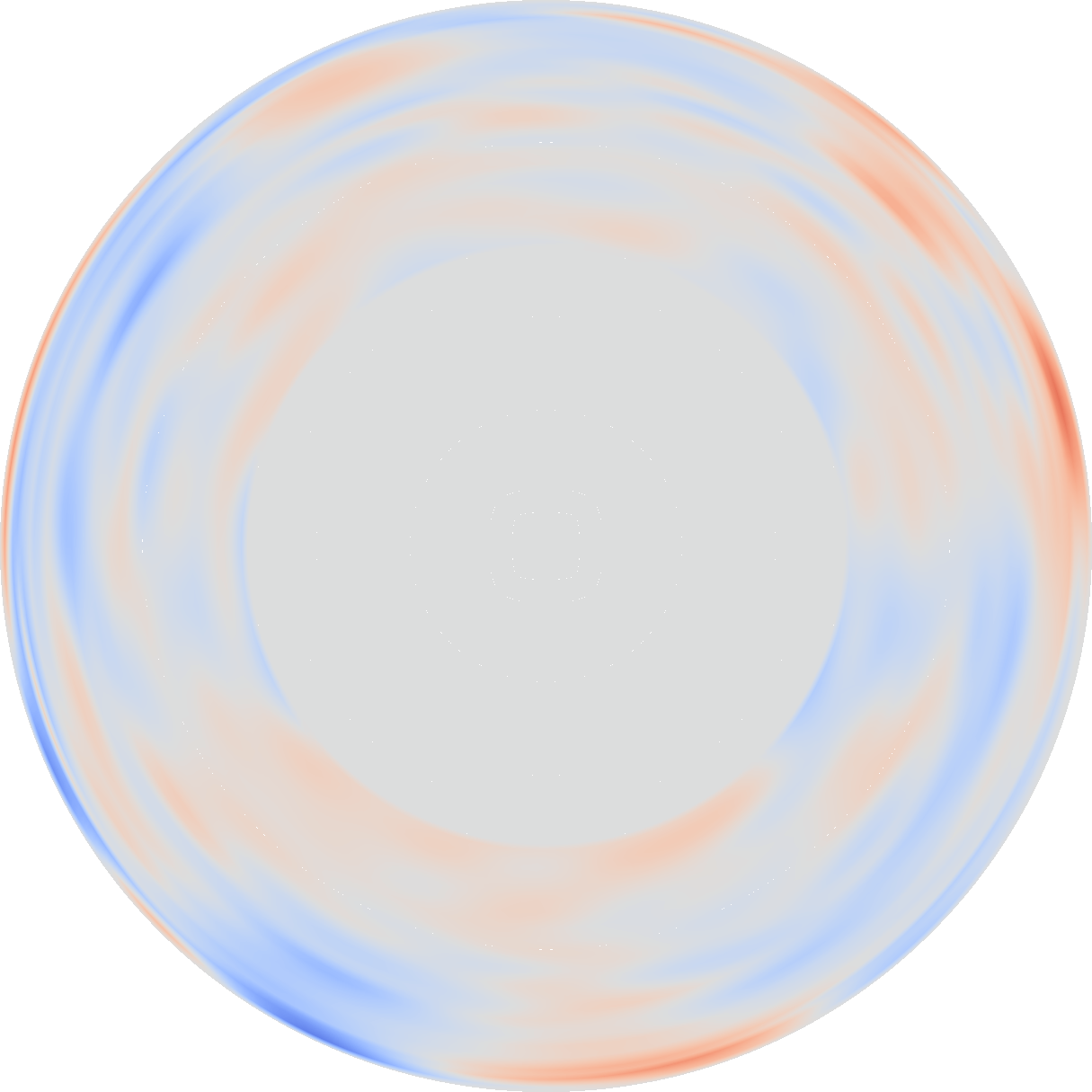
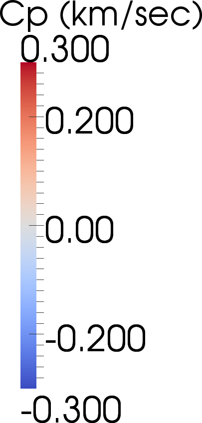
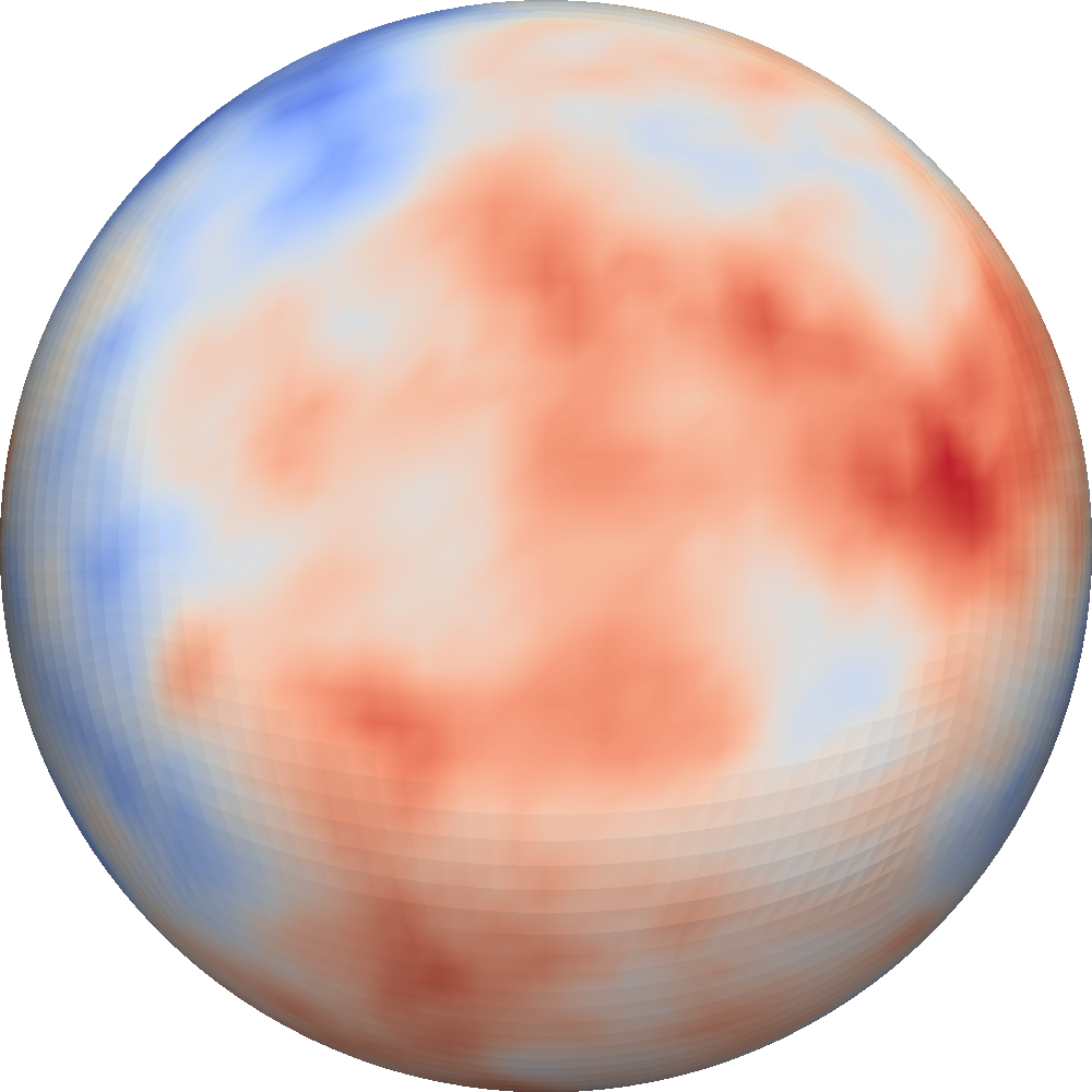
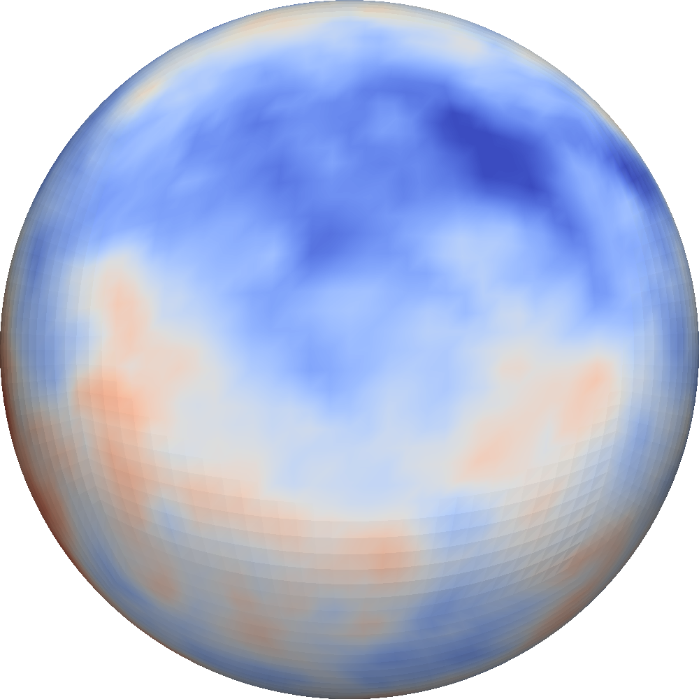
where is the identity matrix, km is the earth radius, , and . The choice introduces anisotropy in such that the prior assumes longer correlation lengths in tangential than in radial directions, and the anisotropy decreases smoothly towards the center of the sphere. In Figure 2 we show several Green’s functions for the precision operator , which illustrate this anisotropy. Figure 3 shows a slice through the fields, through samples from the prior and through the ground truth model, which is used to generate the synthetic seismograms. Note that close to the boundary, the standard deviation of the prior becomes larger. This is partly a results of the anisotropy in the differential operator used in the construction of the prior, but mainly an effect of the homogeneous Neumann boundary condition used in the construction of the square root of the prior. This larger variance close to the boundary is also reflected in the prior samples, which have their largest values close to the boundary. Note that these samples have a larger correlation length in tangential than in normal directions, as intended by the choice of the anisotropy in (32). The ground truth model, which is also shown in Figure 3, is comparable to realizations of the prior in terms of magnitude as well as correlation.


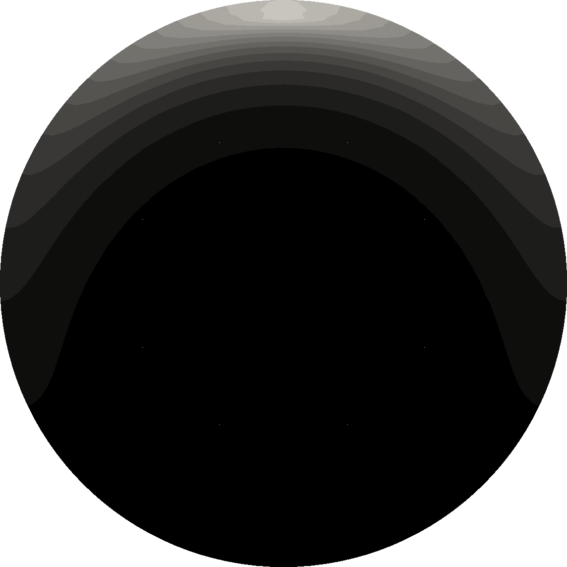
fields
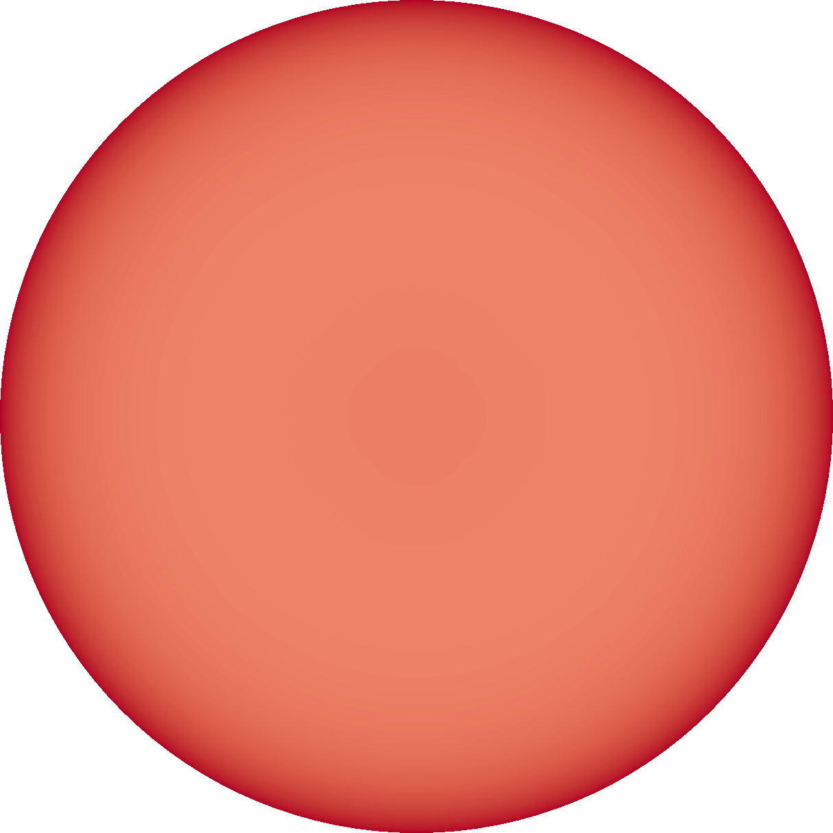

prior samples
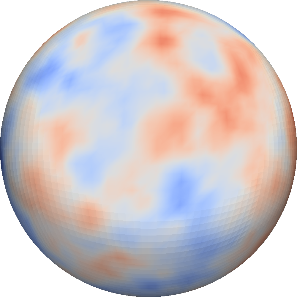
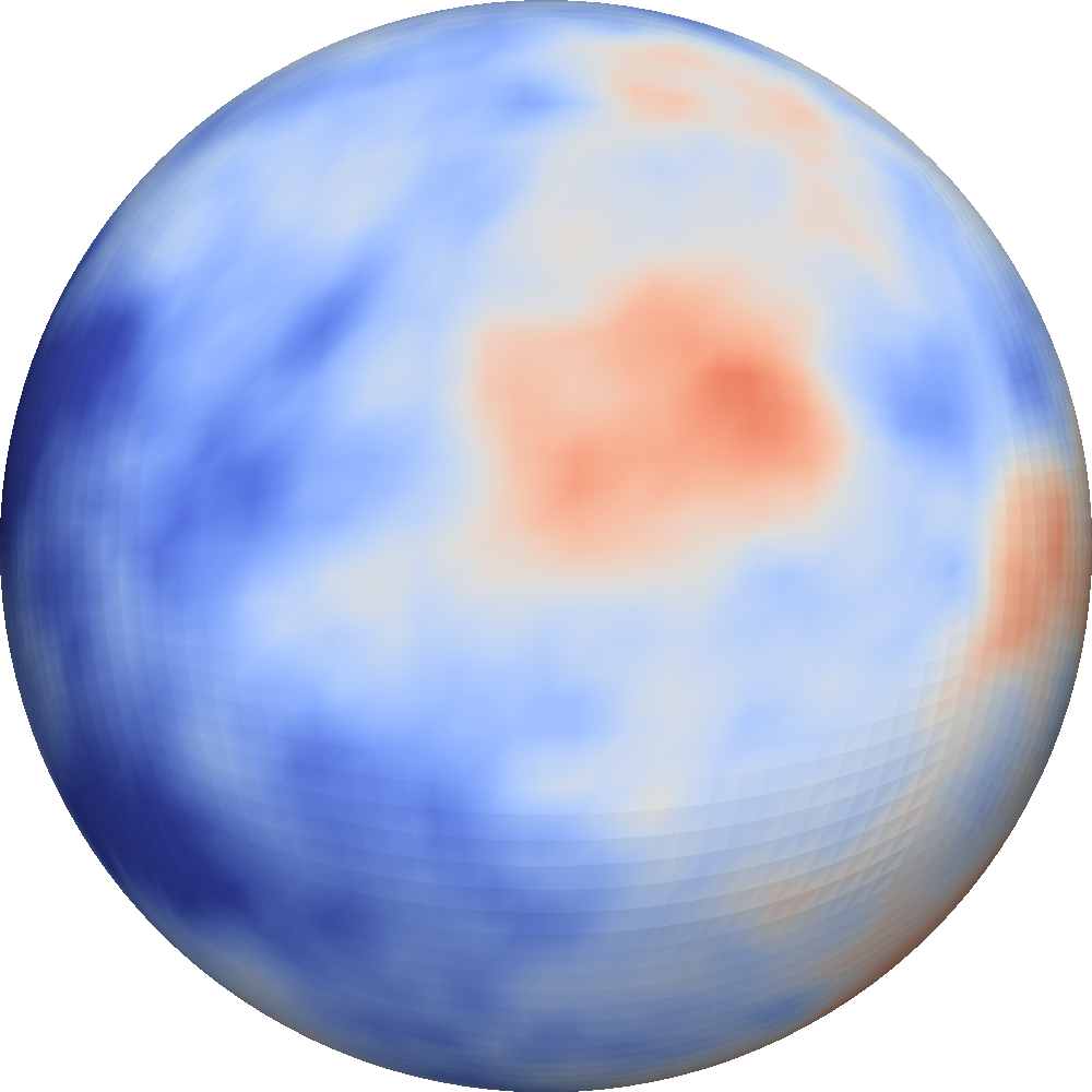
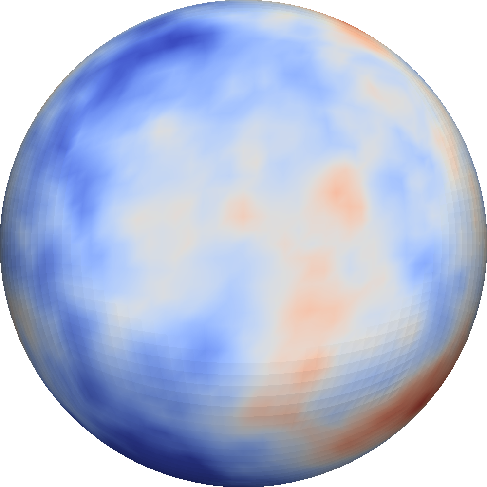
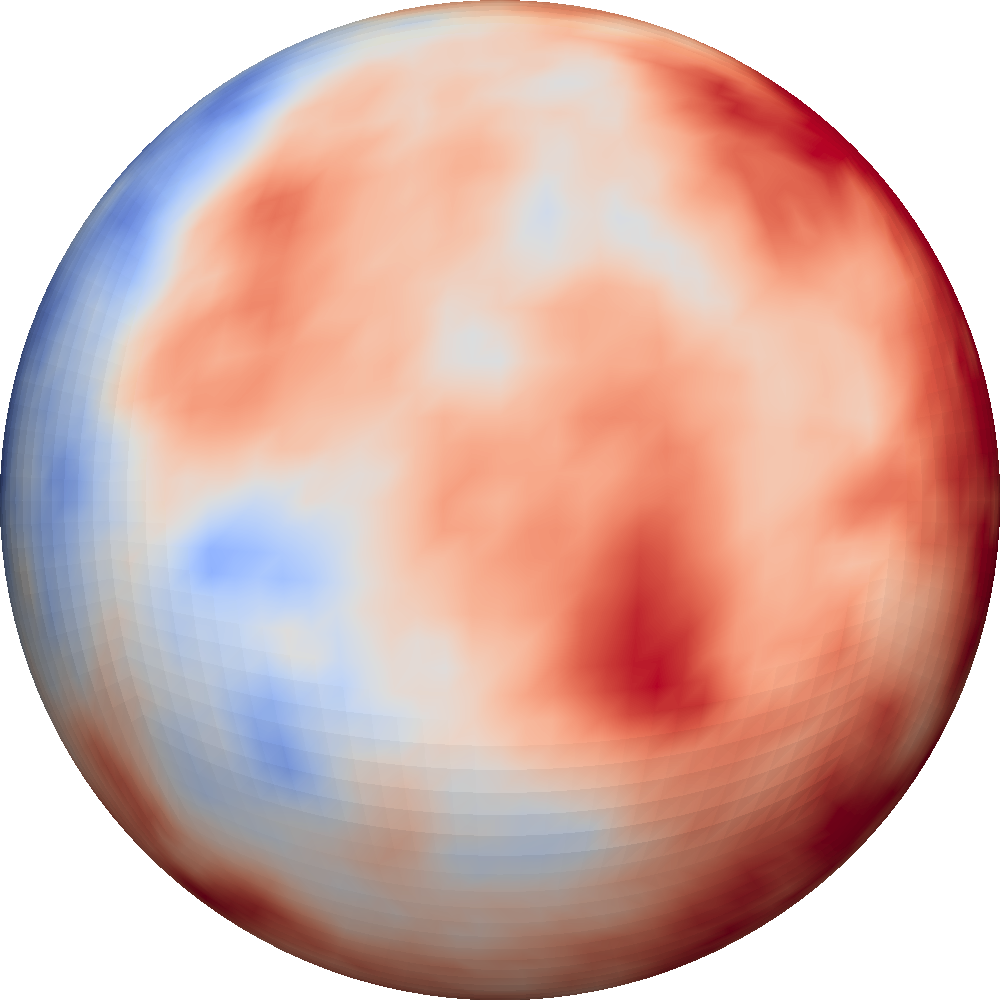
ground truth
6.3 The likelihood
In this section, we construct the likelihood (4) for the inverse acoustic wave problem. In order to do this, we need to construct the parameter-to-observable map and the observations . Let us start by considering the acoustic wave equation written in the first-order form,
| (33a) | ||||
| (33b) | ||||
| where denotes the mass density, the local acoustic wave speed, a (smoothed) point source , the velocity, and the trace of the strain tensor, i.e., the dilatation. We equip (33) with the initial conditions | ||||
| (33c) | ||||
| together with the boundary condition | ||||
| (33d) | ||||
Here, the acoustic wave initial-boundary value problem (33) is a simplified mathematical model for seismic waves propagation in the earth [4]. The choice of strain dilatation together with velocity in the first order system formulation is motivated from the strain-velocity formulation for the elastic wave equation used in [47].
Our goal is to quantify the uncertainty in inferring the spatially varying wave speed from waveforms observed at receiver locations. To define the parameter-to-observable map for a given wave speed , we first solve the acoustic wave equation (33) given , and record the velocity at a finite number of receivers in the time interval . Finally, we compute the Fourier coefficients of the seismograms and truncate them; the truncated coefficients are the observables in the map . A similar procedure is used to generate synthetic seismograms to define . The noise covariance matrix is prescribed as a diagonal matrix with constant variance.
6.4 Gradient and Hessian of the negative log posterior
Our proposed method for uncertainty quantification in Section 3 requires the computation of derivatives of the negative log posterior, which in turn requires the gradient and Hessian of the likelihood and the prior. These derivatives can be computed efficiently using an adjoint method, as we now show. For clarity, we derive the gradient and action of the Hessian in an infinite-dimensional setting. Let us begin by denoting as the space-time solution of the wave equation given the wave speed , and as the observation operator. The parameter-to-observable map can be written as . Thus, the negative log posterior is (compare with (9))
| (34) |
where is specified in Section 6.6. The dependence on the wave speed of the velocity and dilatation is given by the solution of the forward wave propagation equation (33). The adjoint approach [17] allows us to write , the gradient of at a point in parameter space, as
| (35) |
where the adjoint velocity and adjoint strain dilatation satisfy the adjoint wave propagation terminal-boundary value problem
| (36a) | |||||
| (36b) | |||||
| (36c) | |||||
| (36d) | |||||
Here, , an operator from to the space-time cylinder , is the adjoint of . Note that the adjoint wave equations must be solved backward in time (due to final time data) and have the data misfit as a source term, but otherwise resemble the forward wave equations.
Similar to the computation of the gradient, the Hessian operator of at acting on an arbitrary variation is given by
| (37) |
where and satisfy the incremental forward wave propagation initial-boundary value problem
On the other hand, and satisfy the incremental adjoint wave propagation terminal-boundary value problem
As can be seen, the incremental forward and incremental adjoint wave equations are linearizations of their forward and adjoint counterparts, and thus differ only in the source terms. Moreover, we observe that the computation of the gradient and the Hessian action amounts to solving a pair of forward/adjoint and a pair of incremental-forward/incremental-adjoint wave equations, respectively. For our computations, we use the Gauss-Newton approximation of the Hessian, which is guaranteed to be positive. This amounts to neglecting the terms that contain in (37), and neglecting the term that includes in the incremental adjoint wave equations.
6.5 Discretization of the wave equation and implementation details
We use the same hexahedral mesh to compute the wave solution as is used for the parameter . While the parameter is discretized using trilinear finite elements, the wave equation, and its three variants (the adjoint, the incremental forward, and the incremental adjoint), are solved using a high-order discontinuous Galerkin (dG) method. The method, for which details are provided in [47, 9], supports -non-conforming discretization, but only -non-conformity is used in our implementation. For efficiency and scalability, a tensor product of Lagrange polynomials of degree (we use for the examples in the next section) is employed together with a collocation method based on Legendre-Gauss-Lobatto (LGL) nodes. As a result, the mass matrix is diagonal, which facilitates time integration using the classical four-stage fourth-order Runge Kutta method. We equip our dG method with exact Riemann numerical fluxes at element faces. To treat the non-conformity, we use the mortar approach of Kopriva [30, 31] to replace non-conforming faces by mortars that connect pairs of contributing elements. The actual computations are performed on the mortars instead of the non-conforming faces, and the results are then projected onto the contributing element faces. The method has been shown to be consistent, stable, convergent with optimal order, and highly scalable [9, 47].
It should be pointed out that the discretizations of the gradient and Hessian action given in Section 6.4 are not consistent with the discrete gradient and Hessian-vector product obtained by first discretizing the negative log posterior and then differentiating it. Here, inconsistency means that the former are equivalent to the latter only in the limit as the mesh size approaches zero (see also [26, 28]). The reason is that additional jump terms due to numerical fluxes at element interfaces are introduced in the discontinuous Galerkin discretization of the wave equation. In our implementation, we include these terms to ensure consistency, and this is verified by comparing the discretized gradient and Hessian action expressions with their finite difference approximations.
Moreover, since we use a continuous Galerkin finite element method for the parameter, but a discontinuous Galerkin method for the wave solution, it is necessary to prolongate the parameter to the solution space before solving the forward wave equation, and its variants (adjoint, incremental state, incremental adjoint). Conversely, the gradient and the Hessian-vector application are computed in the wave solution space, and then restricted to the parameter space to provide the correct derivatives for the optimization solver. To ensure the symmetry of the Hessian, we construct these restriction and prolongation operations such that they are adjoint of each other.
Our discretization approach for the Bayesian inverse problem in Section 3 requires the repeated application of , each amounting to an elliptic PDE solve on the finite-dimensional parameter space. To accomplish this task efficiently, we use the parallel algebraic multigrid (AMG) solver ML from the Trilinos project [23]. The cost of this elliptic solve is negligible compared to that of solving the time-dependent seismic wave equations, which employ high order discretization in contrast to the trilinear discretization of the anisotropic Poisson operator, .
The adjoint equation has to be solved backwards-in-time (as shown in Section 6.4); computation of the gradient (35) requires combinations of the state and adjoint solutions corresponding to same time. Thus the gradient computation requires the complete time history of the forward solve, which cannot be stored due to the large-scale nature of our problem. A similar, but slightly more challenging storage problem occurs in the Hessian-vector application. Here, solving the incremental state equation requires the solution of the state equation, and the incremental adjoint solution requires the solution of the incremental state equation. We avoid storage of the time history of these wavefields by using a checkpointing method as employed in [17]. This scheme reduces the necessary storage at the expense of increasing the number of wave propagation solves.
Between 1200 and 4096 processor cores333These computations were performed on the Texas Advanced Computing Center’s Lonestar 4 system, which has 22,656 Westmere processor cores with 2GB memory per core. for 10-20 hours are needed to solve the seismic inverse problems presented in the next section. The vast majority of the runtime is spent on computing solutions of the forward, adjoint and incremental wave equations either for the computation of the MAP point (see Section 4) or the Lanczos iterations for computing the low rank approximation of the misfit Hessian (see Section 6.7). Due to the large number of required wave propagation solves, good strong scalability of the wave propagation solver is important for rapid turnaround. We refer to the discussion in [8] on the scalability of the wave propagation solver, as well to the overall scalability of our Bayesian inversion approach applied to seismic inverse problems of up to one million parameters.
6.6 Setup of model problems
Synthetic observations are generated from solution of the wave equation using the S20RTS earth model. To mitigate the inverse crime [29], the local wave speed on LGL nodes of the wave propagation mesh is used to generate the observations, which implies that a higher order approximation of the earth model is used to generate the synthetic data, but the inversion is carried out on a lower order mesh. Both sources and receivers are located at 10km depth from the earth surface. For the source term in (33), we use a delta function point source in the -direction convolved with a narrow Gaussian in space. In time, we employ a Gaussian with standard deviation of s centered at s. The wave propagation mesh (i.e., the discretization of velocity and dilatation) is chosen fine enough to accurately resolve frequencies below Hz. We Fourier transform the (synthetic) observed velocity waveforms at each receiver location and retain only the first 101 Fourier modes to define the observations . In our problems, the Fourier coefficients vary between and , and we choose for the noise covariance a diagonal matrix with a standard deviation of .
We consider the following two model problems:
-
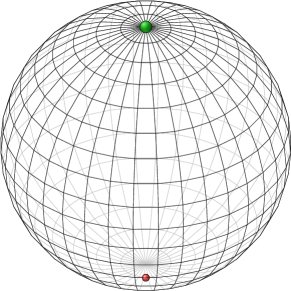
•
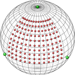
Problem I: The first problem has a single source at the North pole and a single receiver at 45∘ south of the equator, as illustrated in the left image of Figure 4. The wave propagation time is 1800s. The wave speed (i.e., unknown material parameter) field is discretized on a mesh of trilinear hexahedra with 78,558 nodes, representing the unknowns in the inverse problem. The forward problem is discretized on the same mesh with 3rd-order dG elements, resulting in about 21.4 million spatial wave propagation unknowns, and in 2100 four-stage, fourth-order Runge Kutta time steps.
-
•
Problem II: The second problem uses 130 receivers distributed on a quarter of the Northern hemisphere along zonal lines with 7.5∘ spacing and 3 simultaneous sources as shown on the right of Figure 4. The wave propagation time is 1200s. The wave speed is discretized on three different trilinear hexahedral meshes with 40,842, 67,770 and 431,749 wave speed parameters, which represent the unknowns in the inverse problem. These meshes corresponding to discretizations with 4th, 3rd and 2nd order discontinuous elements for the wave propagation variables (velocity and dilatation). The results in the next section were computed with 67,770 wave speed parameters and the 3rd order dG discretization for velocity and dilatation. This amounts to 18.7 million spatial wave propagation unknowns, and 1248 Runge Kutta time steps.
6.7 Low rank approximation of the prior-preconditioned misfit Hessian
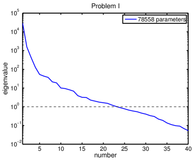
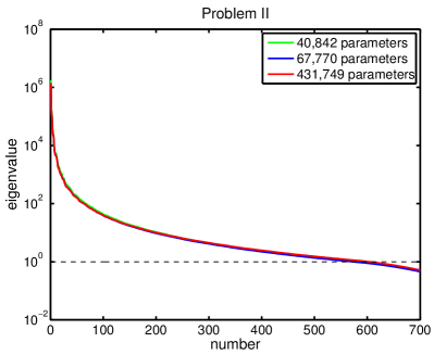
Before discussing the results for the quantification of the uncertainty in the solution of our inverse problems, we numerically study the spectrum of the prior-preconditioned misfit Hessian. In Figure 5, we show the dominant spectrum of the prior-preconditioned Hessian evaluated at the MAP estimate for Problem I (left) and Problem II (right). As can be observed, the eigenvalues decay faster in the former than in the latter. That is, the former is more ill-posed than the latter. The reason is that the three simultaneous source and 130 receivers of Problem II provide more information on the earth model. This implies that retaining more eigenvalues is necessary to accurately approximate the prior-preconditioned Hessian of the data misfit for Problem II compared to Problem I. In particular, we need at least 700 eigenvalues for Problem II as compared to about 40 for Problem I to obtain a sensible low-rank approximation of the Hessian, and this constitutes the bulk of computation time (since each Hessian-vector product in the Lanczos solver requires incremental forward and adjoint wave propagation solutions). These numbers compare with a total number of parameters of 78,558 (Problem I) and 67,770 (Problem II), which amounts to a reduction of between two and three orders of magnitude. This directly translates into two to three orders of magnitude reduction in cost of solving the statistical inverse problem.
Figure 5 presents the spectra for Problem II for three different discretization of the wave speed parameter field. The figure suggests that the dominant spectrum is essentially mesh-independent and that all three parameter meshes are sufficiently fine to resolve the dominant eigenvectors of the prior-preconditioned Hessian. Consequently, the Hessian low-rank approximation, particularly the number of Lanczos iterations, is independent of the number of discrete parameters. Thus, in this example, the number of wave propagation solutions required by the low-rank approximation does not depend on the parameter dimension.
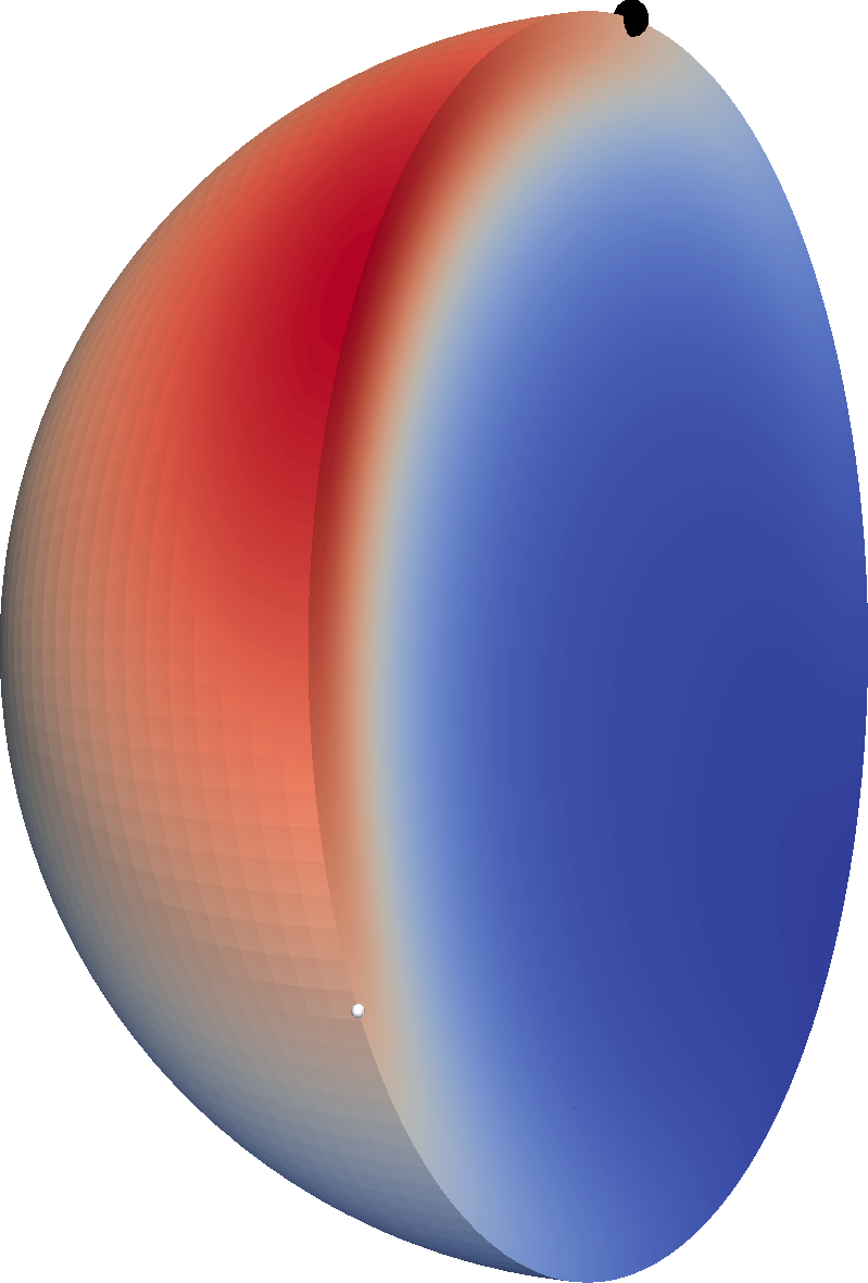
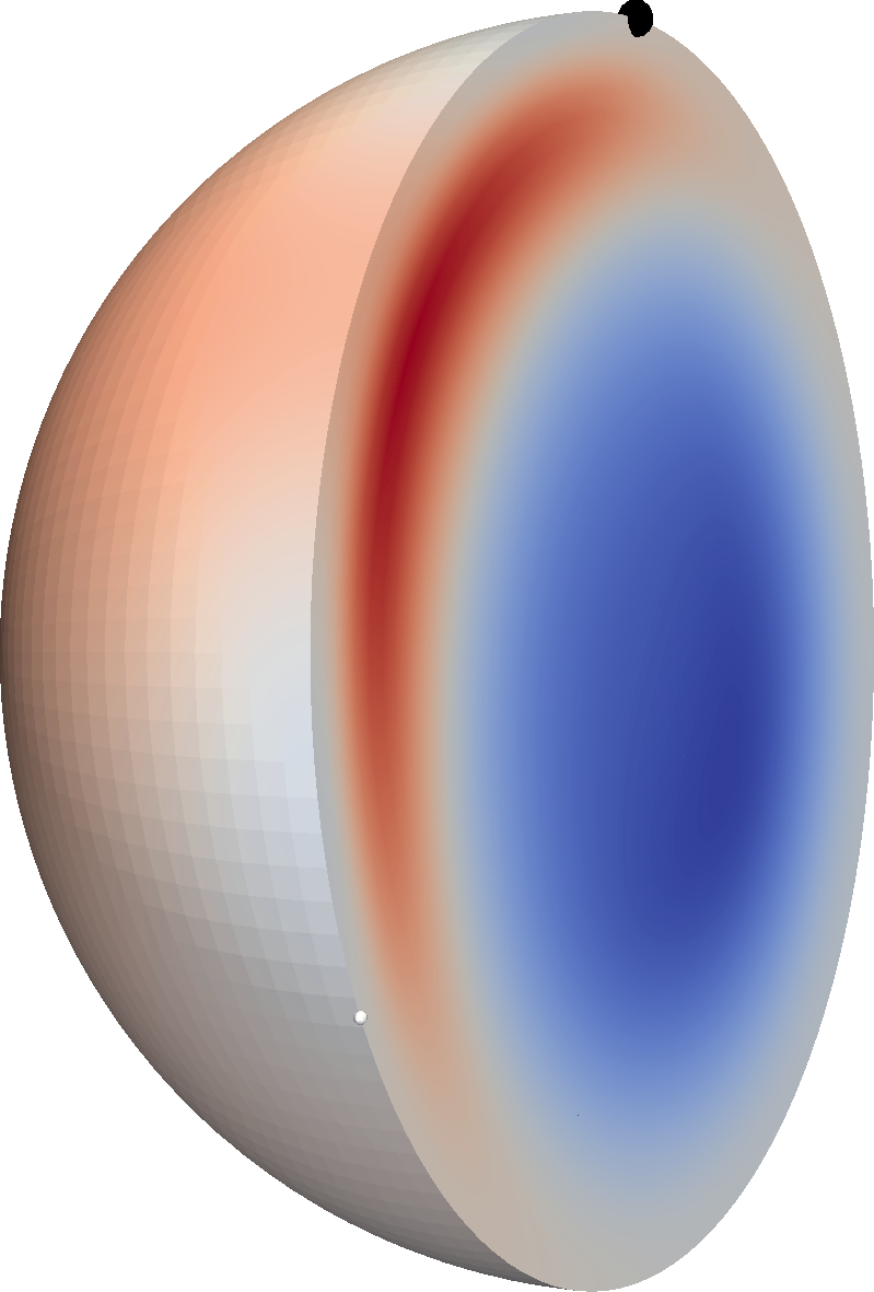
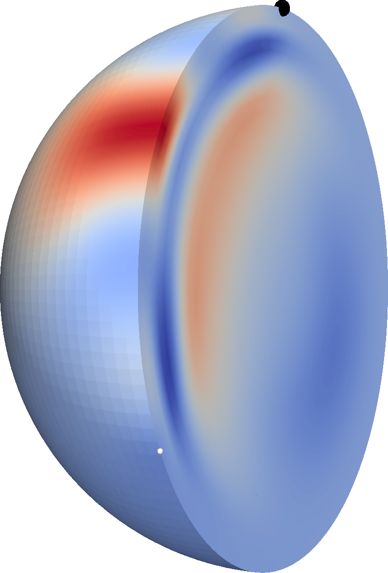
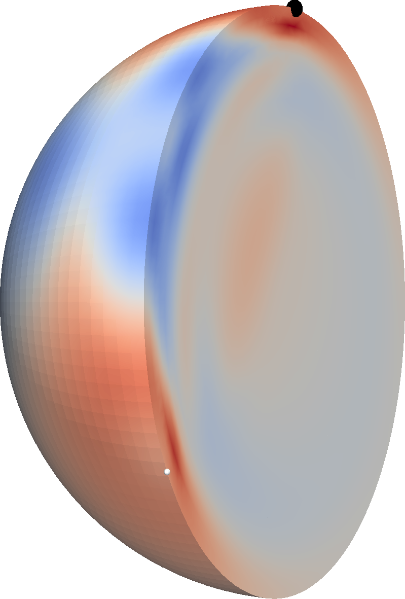
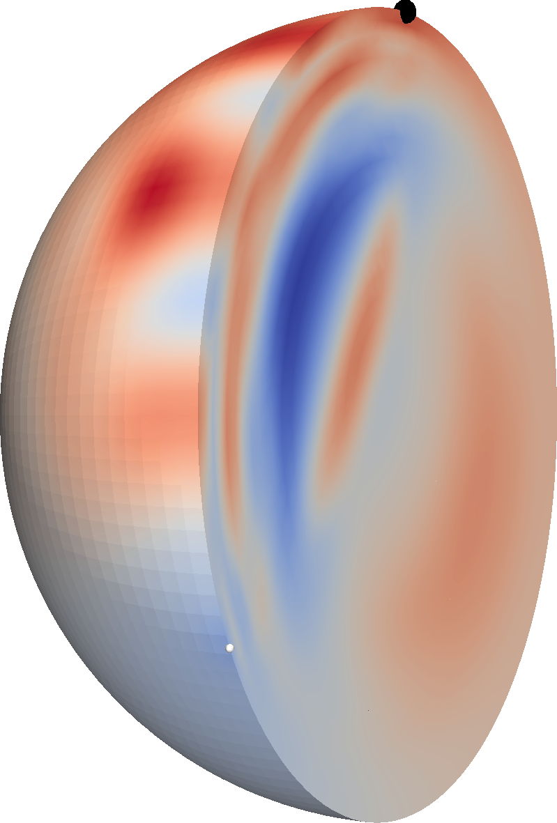
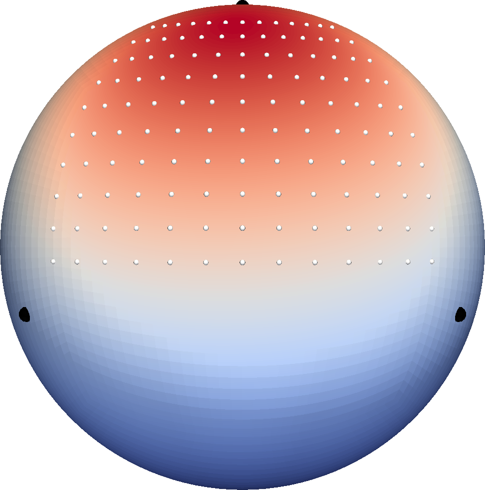
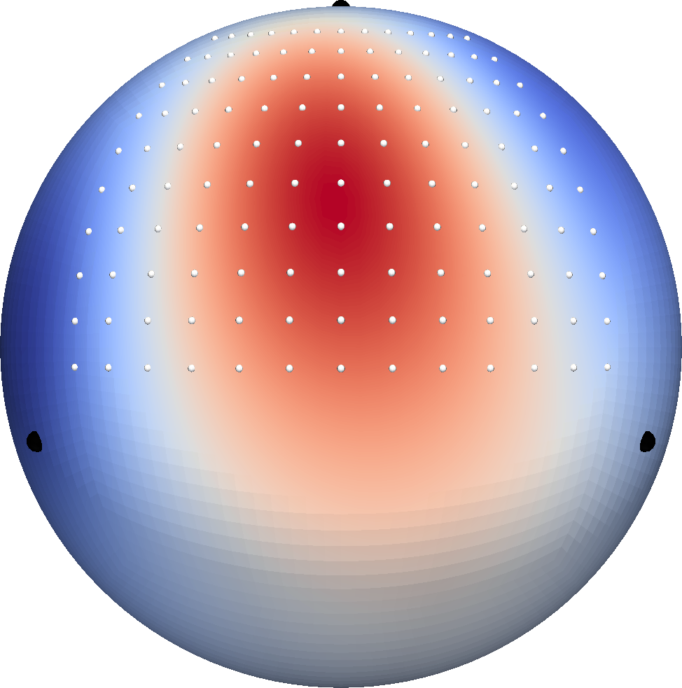
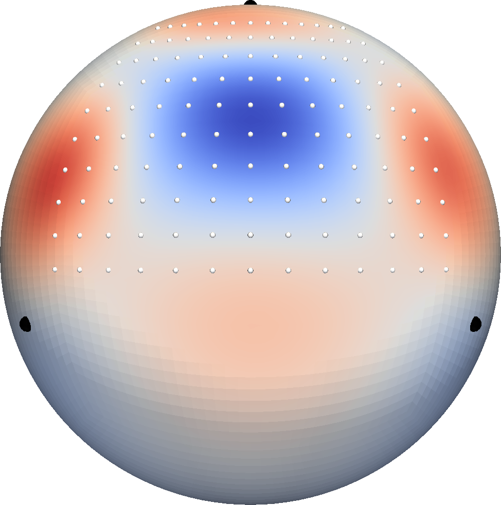
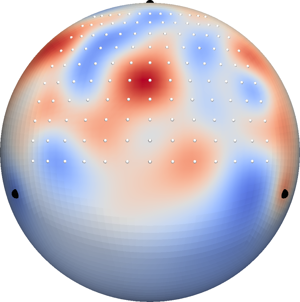
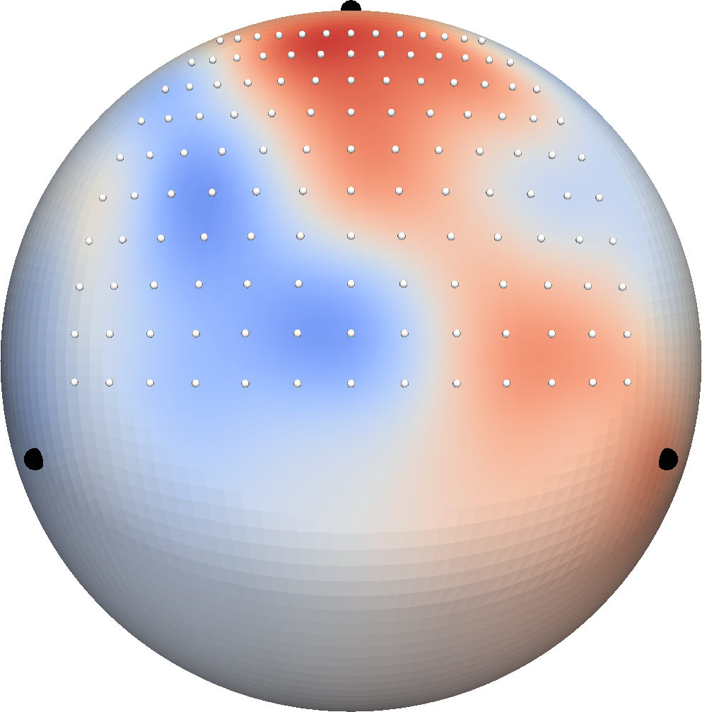
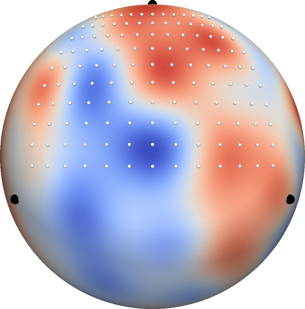
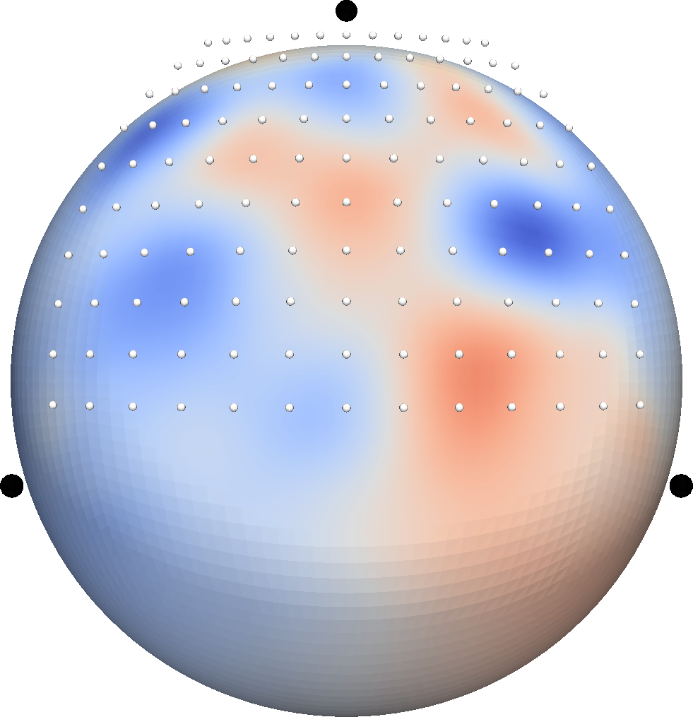
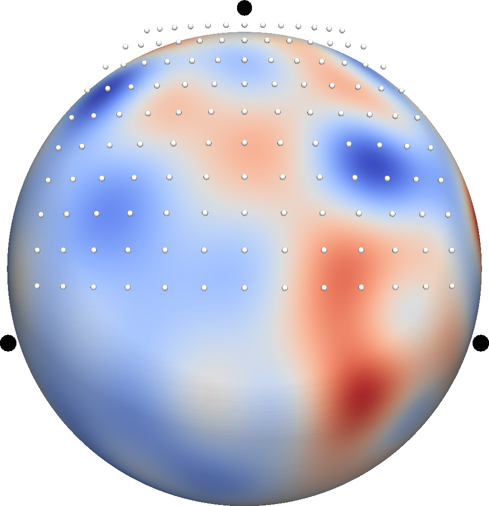
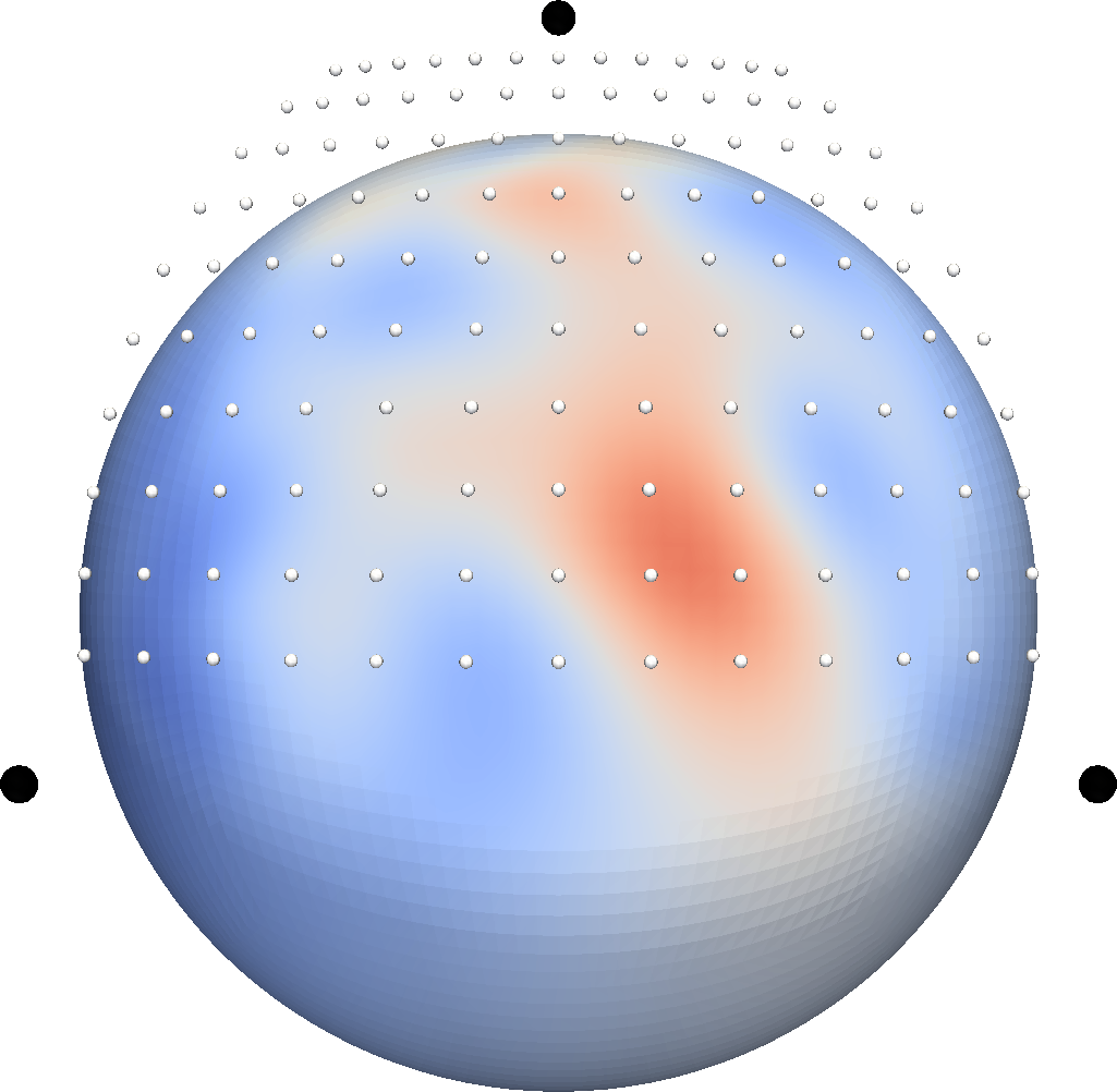
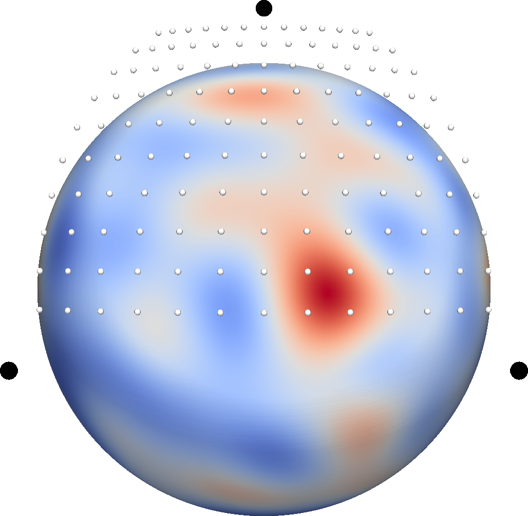
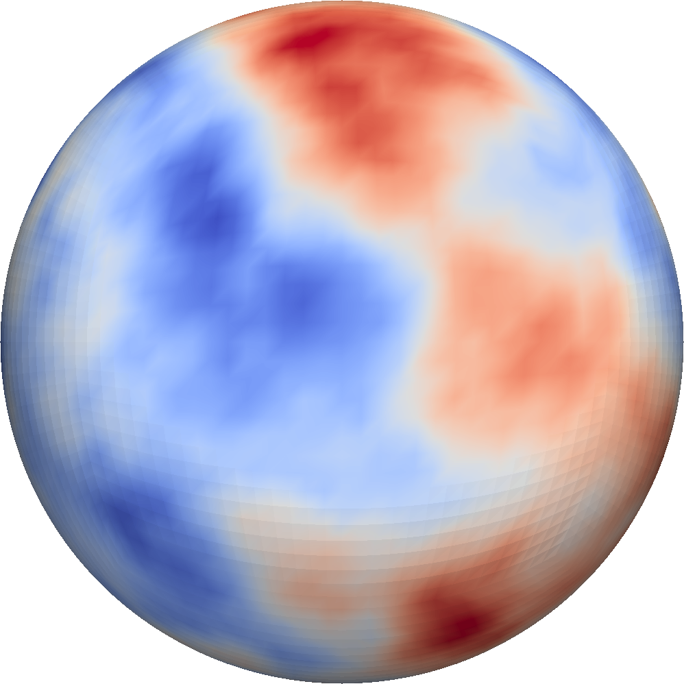
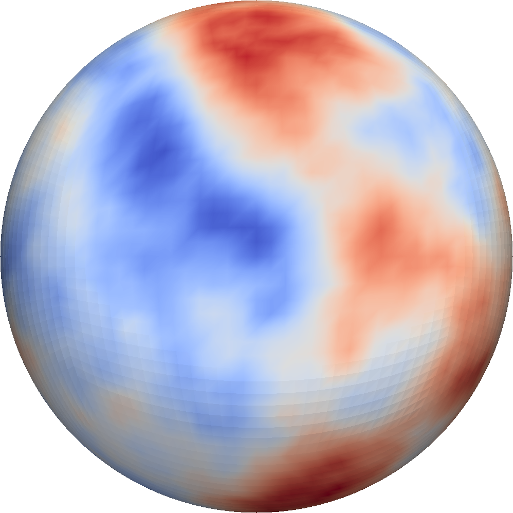
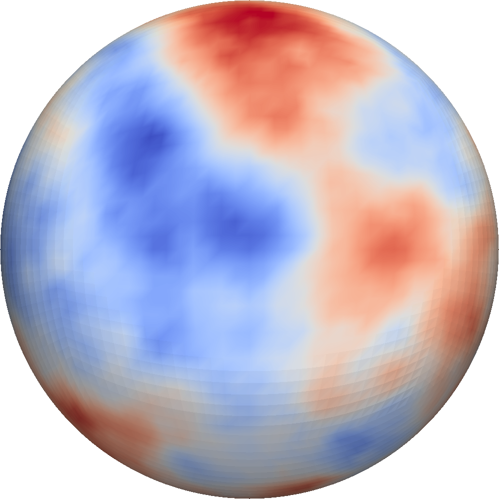
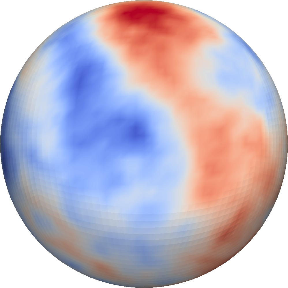
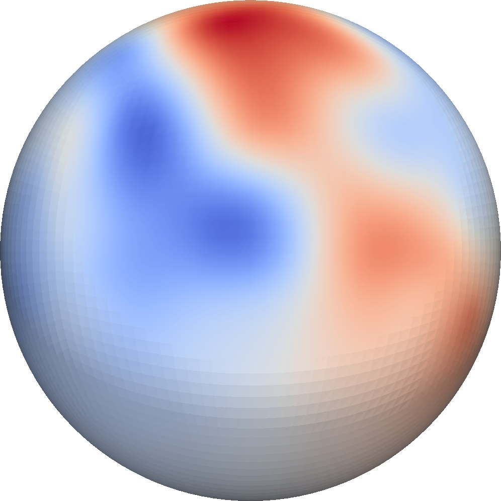
Figures 6 and 7 show several eigenvectors of the prior preconditioned data misfit Hessian (23) (corresponding to several dominant eigenvalues) for Problems I and II. Eigenvectors corresponding to dominant eigenvalues represent the earth modes that are “most observable” from the data, given the configuration of sources and receivers. As can be seen in these figures, the largest eigenvalues produce the smoothest modes, and as the eigenvalues decrease, the associated eigenvectors become more oscillatory, due to the reduced ability to infer smaller length scales from the observations.
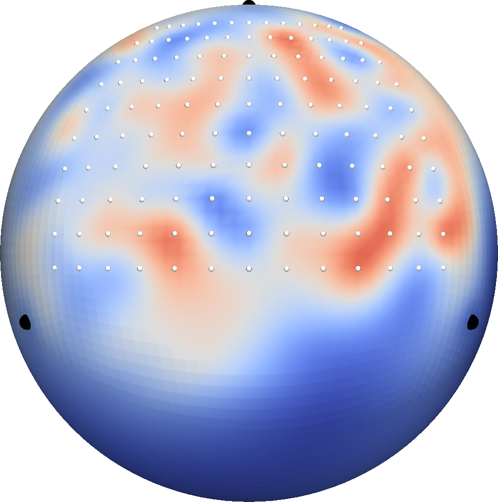
6.8 Interpretation of the uncertainty in the solution of the inverse problem
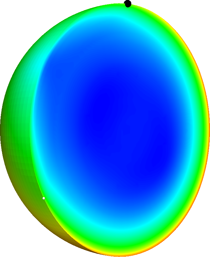
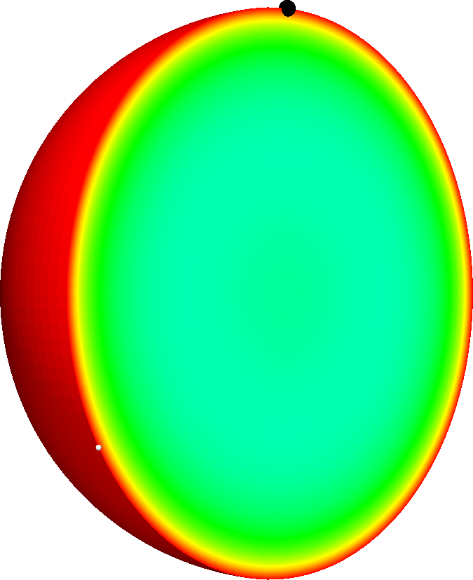
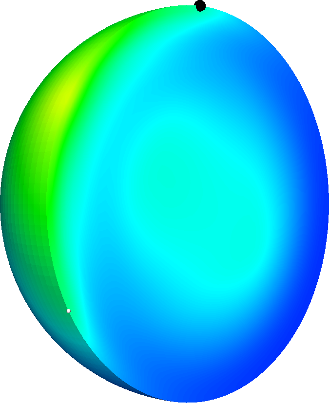
We first study Problem I, i.e., the single source, single receiver problem. Since the data are very sparse, it is expected that we can reconstruct only very limited information from the truth solution; this is reflected in the smoothness of the dominant eigenmodes shown in Figure 6. To assess the uncertainty, Figure 8 shows prior variance, knowledge gained from the data (i.e., reduction in the variance), and posterior variance, which are computed from (29). As discussed in Section 5, the posterior is the combination of the prior information and the knowledge gained from the data, so that the posterior uncertainty is decreased relative to the prior uncertainty. That is, the inference has less uncertainty in regions for which the data are more informative. In particular, the region of lowest uncertainty is at the surface half-way between source and receiver, as Figure 8 shows. Note that the data are also informative about the core-mantle boundary, where the strong material contrast results in stronger reflected energy back to the surface receivers, allowing greater confidence in the properties of that interface.
Next, we study the results for Problem II. The comparison between the MAP estimate and the ground truth earth model (S20RTS) at different depths is displayed in Figure 9. As can be seen, we are able to recover accurately the wave speed in the portion of the Northern hemisphere covered by sources and receivers. We plot the prior and posterior pointwise standard deviations in Figure 10. One observes that the uncertainty reduction is greatest along the wave paths between sources and receivers, particularly in the quarter of the Northern hemisphere surface where the receivers are distributed.
In Figure 11, we show a comparison between samples from the prior distribution and from the posterior. We observe that in the quarter of the Northern hemisphere where the data are more informative about the medium, we have a higher degree of confidence about the wave speed, which is manifested in the common large scale features across the posterior samples. The fine-scale features (about which the data are least informative) are qualitatively similar to those of the prior distribution, and vary from sample to sample in the posterior. We note that the samples shown here are computed by approximating in expression (30) using the (diagonal) lumped mass matrix to avoid computing a factorization of . If desired, this mass lumping can be avoided by applying to a vector using an iterative scheme based on polynomial approximations to the matrix function , as in [14].

7 Conclusions
A computational framework for estimating the uncertainty in the numerical solution of linearized infinite-dimensional statistical inverse problems is presented. We adopt the Bayesian inference formulation: given observational data and their uncertainty, the governing forward problem and its uncertainty, and a prior probability distribution describing uncertainty in the parameter field, find the posterior probability distribution over the parameter field. The framework, which builds on the infinite-dimensional formulation proposed by Stuart [42], incorporates a number of components aimed at ensuring a convergent discretization of the underlying infinite-dimensional inverse problem. It additionally incorporates algorithms for manipulating the prior, constructing a low rank approximation of the data-informed component of the posterior covariance operator, and exploring the posterior, that together ensure scalability of the entire framework to very high parameter dimensions. Since the data are typically informative about only a low dimensional subspace of the parameter space, the Hessian is sparse with respect to some basis. We have exploited this fact to construct a low rank approximation of the Hessian and its inverse using a parallel matrix-free Lanczos method. Overall, our method requires a dimension-independent number of forward PDE solves to approximate the local covariance. Uncertainty quantification for the linearized inverse problem thus reduces to solving a fixed number of forward and adjoint PDEs (which resemble the original forward problem), independent of the problem dimension. The entire process is thus scalable with respect to the forward problem dimension, uncertain parameter dimension, and observational data dimension. We applied this method to the Bayesian solution of an inverse problem in 3D global seismic wave propagation with up to 430,000 parameters, for which we observe 2–3 orders of magnitude dimension reduction, making UQ for large-scale inverse problems tractable.
Appendix
In the following, we provide a constructive derivation of in (30) such that it satisfies . Our goal is to draw posterior Gaussian random sample with covariance matrix in . To accomplish this, a standard approach is first to find a factorization , where is a linear map from to . Then, any random sample from the posterior can be written as
| (38) |
where is a Gaussian random sample with zero mean and identity covariance matrix in . It follows that
where is the standard Gaussian random sample with zero mean and identity covariance matrix in , i.e. , and a linear map from to .
Therefore, what remains to be done is to construct . To begin the construction, we rewrite (28) as
The simple structure of allows us to write its spectral decomposition as
which, together with the standard definition of the square root of postive self-adjoint operators [5], immediately gives
where , and is self-adjoint in , namely, . Now, we define
which, by construction, is the desired matrix owing to the following trivial identity
where we have used the self-adjointness of and in .
Finally, we can rewrite (38) in terms of and , a linear map from to , as
where satisfies the following desired identity
References
- [1] Petter Abrahamsen, A review of Gaussian random fields and correlation functions, Tech. Report 2nd edition, Norwegian Computing Center, Box 114, Blindern N-0314 Oslo, Norway, 1997.
- [2] Volkan Akçelik, Jacobo Bielak, George Biros, Ioannis Epanomeritakis, Antonio Fernandez, Omar Ghattas, Eui J. Kim, Julio Lopez, David R. O’Hallaron, Tiankai Tu, and John Urbanic, High resolution forward and inverse earthquake modeling on terascale computers, in SC03: Proceedings of the International Conference for High Performance Computing, Networking, Storage, and Analysis, ACM/IEEE, 2003. Gordon Bell Prize for Special Achievement.
- [3] Volkan Akçelik, George Biros, and Omar Ghattas, Parallel multiscale Gauss-Newton-Krylov methods for inverse wave propagation, in Proceedings of IEEE/ACM SC2002 Conference, Baltimore, MD, Nov. 2002. SC2002 Best Technical Paper Award.
- [4] Keiiti Aki and Paul G. Richards, Quantitative Seismology, University Science Books, 2nd ed., 2002.
- [5] Todd Arbogast and Jerry L. Bona, Methods of Applied Mathematics, University of Texas at Austin, 2008. Lecture notes in applied mathematics.
- [6] Johnathan M. Bardsley, Gaussian Markov random field priors for inverse problems, Inverse Problems and Imaging, (2013).
- [7] Alexandros Beskos, Gareth Roberts, and Andrew Stuart, Optimal scalings for local Metropolis-Hastings chains on nonproduct targets in high dimensions, The Annals of Applied Probability, 19 (2009), pp. 863–898.
- [8] Tan Bui-Thanh, Carsten Burstedde, Omar Ghattas, James Martin, Georg Stadler, and Lucas C. Wilcox, Extreme-scale UQ for Bayesian inverse problems governed by PDEs, in SC12: Proceedings of the International Conference for High Performance Computing, Networking, Storage and Analysis, 2012.
- [9] Tan Bui-Thanh and Omar Ghattas, Analysis of an -non-conforming discontinuous Galerkin spectral element method for wave propagation, SIAM Journal on Numerical Analysis, 50 (2012), pp. 1801–1826.
- [10] , Analysis of the Hessian for inverse scattering problems. Part I: Inverse shape scattering of acoustic waves, Inverse Problems, 28 (2012), p. 055001.
- [11] , Analysis of the Hessian for inverse scattering problems. Part II: Inverse medium scattering of acoustic waves, Inverse Problems, 28 (2012), p. 055002.
- [12] Carsten Burstedde, Omar Ghattas, Michael Gurnis, Tobin Isaac, Georg Stadler, Tim Warburton, and Lucas C. Wilcox, Extreme-scale AMR, in SC10: Proceedings of the International Conference for High Performance Computing, Networking, Storage and Analysis, ACM/IEEE, 2010.
- [13] Carsten Burstedde, Lucas C. Wilcox, and Omar Ghattas, p4est: Scalable algorithms for parallel adaptive mesh refinement on forests of octrees, SIAM Journal on Scientific Computing, 33 (2011), pp. 1103–1133.
- [14] Jie Chen, Mihai Anitescu, and Yousef Saad, Computing via least squares polynomial approximations, SIAM Journal on Scientific Computing, 33 (2011), pp. 195–222.
- [15] David Colton and Rainer Kress, Inverse Acoustic and Electromagnetic Scattering, Applied Mathematical Sciences, Vol. 93, Springer-Verlag, Berlin, Heidelberg, New-York, Tokyo, second ed., 1998.
- [16] Adam M. Dziewonski and Don L. Anderson, Preliminary reference earth model, Physics of the Earth and Planetary Interiors, 25 (1981), pp. 297–356.
- [17] Ioannis Epanomeritakis, Volkan Akçelik, Omar Ghattas, and Jacobo Bielak, A Newton-CG method for large-scale three-dimensional elastic full-waveform seismic inversion, Inverse Problems, 24 (2008), p. 034015 (26pp).
- [18] Lawerence C. Evans, Partial Differential Equations, American Mathematical Society, Providence, RI, 1998.
- [19] Andreas Fichtner, Full seismic waveform modelling and inversion, Springer, 2011.
- [20] Andreas Fichtner, Heiner Igel, Hans-Peter Bunge, and Brian L. N. Kennett, Simulation and inversion of seismic wave propagation on continental scales based on a spectral-element method, Journal of Numerical Analysis, Industrial and Applied Mathematics, 4 (2009), pp. 11–22.
- [21] Andreas Fichtner, Brian L. N. Kennett, Heiner Igel, and Hans-Peter Bunge, Full waveform tomography for upper-mantle structure in the Australasian region using adjoint methods, Geophysical Journal International, 179 (2009), pp. 1703–1725.
- [22] H. Pearl Flath, Lucas C. Wilcox, Volkan Akçelik, Judy Hill, Bart van Bloemen Waanders, and Omar Ghattas, Fast algorithms for Bayesian uncertainty quantification in large-scale linear inverse problems based on low-rank partial Hessian approximations, SIAM Journal on Scientific Computing, 33 (2011), pp. 407–432.
- [23] Michael W. Gee, Christopher M. Siefert, Jonathan J. Hu, Ray S. Tuminaro, and Marzion G. Sala, ML 5.0 smoothed aggregation user’s guide, Tech. Report SAND2006-2649, Sandia National Laboratories, 2006.
- [24] Andrew Gelman, John B. Carlin, Hal S. Stern, and Donald B. Rubin, Bayesian Data Analysis, Second Edition (Chapman & Hall/CRC Texts in Statistical Science), Chapman and Hall/CRC, 2 ed., July 2003.
- [25] Mark Girolami and Ben Calderhead, Riemann manifold Langevin and Hamiltonian Monte Carlo methods, Journal of the Royal Statistical Society: Series B (Statistical Methodology), 73 (2011), pp. 123–214.
- [26] Max D. Gunzburger, Perspectives in Flow Control and Optimization, SIAM, Philadelphia, 2003.
- [27] Martin Hairer, Introduction to Stochastic PDEs. Lecture Notes, 2009.
- [28] Michael Hinze, Rene Pinnau, Michael Ulbrich, and Stefan Ulbrich, Optimization with PDE Constraints, Springer, 2009.
- [29] Jari Kaipio and Erkki Somersalo, Statistical and Computational Inverse Problems, vol. 160 of Applied Mathematical Sciences, Springer-Verlag, New York, 2005.
- [30] David A. Kopriva, A conservative staggered-grid Chebyshev multidomain method for compressible flows. II. A semi-structured method, Journal of Computational Physics, 128 (1996), pp. 475–488.
- [31] David A. Kopriva, Stephen L. Woodruff, and M. Yousuff Hussaini, Computation of electromagnetic scattering with a non-conforming discontinuous spectral element method, International Journal for Numerical Methods in Engineering, 53 (2002), pp. 105–122.
- [32] Matti Lassas, Eero Saksman, and Samuli Siltanen, Discretization invariant Bayesian inversion and Besov space priors, Inverse Problems and Imaging, 3 (2009), pp. 87–122.
- [33] Lucien LeCam, Asymptotic Methods in Statistical Decision Theory, Springer, 1986.
- [34] Vedran Lekić and Barbara Romanowicz, Inferring upper-mantle structure by full waveform tomography with the spectral element method, Geophysical Journal International, 185 (2011), pp. 799–831.
- [35] Finn Lindgren, Håvard Rue, and Johan Lindström, An explicit link between gaussian fields and gaussian markov random fields: the stochastic partial differential equation approach, Journal of the Royal Statistical Society: Series B (Statistical Methodology), 73 (2011), pp. 423–498.
- [36] James Martin, Lucas C. Wilcox, Carsten Burstedde, and Omar Ghattas, A stochastic Newton MCMC method for large-scale statistical inverse problems with application to seismic inversion, SIAM Journal on Scientific Computing, 34 (2012), pp. A1460–A1487.
- [37] Daniel Peter, Dimitri Komatitsch, Yang Luo, Roland Martin, Nicolas Le Goff, Emanuele Casarotti, Pieyre Le Loher, Federica Magnoni, Qinya Liu, Celine Blitz, Tarje Nisson-Meyer, Piero Basini, and Jeroen Tromp, Forward and adjoint simulations of seismic wave propagation on fully unstructured hexahedral meshes, Geophysical Journal International, 186 (2011), pp. 721–739.
- [38] Jeroen Ritsema and Jan Van Heijst, Constraints on the correlation of p-and s-wave velocity heterogeneity in the mantle from p, pp, ppp and pkpab traveltimes, Geophysical Journal International, 149 (2002), pp. 482–489.
- [39] Christian P. Robert and George Casella, Monte Carlo Statistical Methods (Springer Texts in Statistics), Springer-Verlag New York, Inc., Secaucus, NJ, USA, 2005.
- [40] Havard Rue, Fast sampling of gaussian markov random fields, Journal of the Royal Statistical Society: Series B (Statistical Methodology), 63 (2001), pp. 325–338.
- [41] Havard Rue and Leonhard Held, Gaussian Markov random fields: theory and applications, vol. 104, Chapman & Hall, 2005.
- [42] Andrew M. Stuart, Inverse problems: A Bayesian perspective, Acta Numerica, 19 (2010), pp. 451–559.
- [43] Carl Tape, Qinya Liu, Alessia Maggi, and Jeroen Tromp, Adjoint tomography of the southern California crust, Science, 325 (2009), pp. 988–992.
- [44] Albert Tarantola, Inverse Problem Theory and Methods for Model Parameter Estimation, SIAM, Philadelphia, PA, 2005.
- [45] Curt R. Vogel, Computational Methods for Inverse Problems, Frontiers in Applied Mathematics, Society for Industrial and Applied Mathematics (SIAM), Philadelphia, PA, 2002.
- [46] Jochen Voss, The effect of finite element discretisation on the stationary distribution of SPDEs, Communications in Mathematical Sciences, 10 (2012), pp. 1143–1159.
- [47] Lucas C. Wilcox, Georg Stadler, Carsten Burstedde, and Omar Ghattas, A high-order discontinuous Galerkin method for wave propagation through coupled elastic-acoustic media, Journal of Computational Physics, 229 (2010), pp. 9373–9396.
- [48] Hejun Zhu, Ebru Bozdapg, Daniel Peter, and Jeroen Tromp, Structure of the European upper mantle revealed by adjoint tomography, Nature Geoscience, 5 (2012), pp. 493–498.