Static Solutions of Einstein’s Equations with Spherical Symmetry

Abstract

The Schwarzschild solution is a complete solution of Einstein’s field equations for a static spherically symmetric field. The Einstein’s field equations solutions appear in the literature, but in different ways corresponding to different definitions of the radial coordinate. We attempt to compare them to the solutions with nonvanishing energy density and pressure. We also calculate some special cases with changes in spherical symmetry.

Keywords: Schwarzschild solution, Spherical symmetry, Einstein’s equations, Static universe.

1 Introduction

Even though the Einstein field equations are highly nonlinear partial differential equations, there are numerous exact solutions to them. In addition to the exact solution, there are also non-exact solutions to these equations which describe certain physical systems. Exact solutions and their physical interpretations are sometimes even harder. Probably the simplest of all exact solutions to the Einstein field equations is that of Schwarzschild. Furthermore, the static solutions of Einstein’s equations with spherical symmetry (the exterior and interior Schwarzschild solutions) are already much popular in general relativity, solutions with spherical symmetry in vacuum are much less recognizable. Together with conventional isometries, which have been more widely studied, they help to provide a deeper insight into the spacetime geometry. They assist in the generation of exact solutions, sometimes new solutions of the Einstein field equations which may be utilized to model relativistic, astrophysical and cosmological phenomena. Stephani et al.([1])has emphasized the role of symmetries in classifying and categorizing exact solutions.
Symmetries are used as one of the principal classification schemes in their catalogue of known solutions. In this paper we construct the vacuum solutions of this sort, and we set up the differential equations for nonvacuum solutions. Indeed, to some extent more general vacuum solutions, possibly breaking the translational invariance, were found in the early $20th$ century by Weyl and Levi-Civita ([2] [3]), and their analogs breaking the static condition were studied by Rosen and Marder [4] in mid-century. Afterward, much attention was given to “cosmic strings” thin cylinders (usually filled with a non-Abelian gauge field) surrounded by vacuum (e.g. [[5]-[7]]).

In this paper the metric obtained describes the solution in vacuum due to spherically symmetric distribution of matter. The field is static and can be produced by spherically symmetric motion. The requirement of spherical symmetry alone is sufficient to yield the static nature of our solution. Moreover, the metric tensor tends to approach the Minkowskian flat spacetime metric tensor, and also the well known cosmic string solutions are locally flat (;regular Minkowskian spacetime minus a wedge described by a deficit angle). It is not widely appreciated that the static, translationally invariant cases of the older solutions ( [2],[3],[4] ) are not all of that type.
We write the most general expression for a spacetime metric with static and spherical symmetry and solve the Einstein field equations for the components of the metric tensor. We carefully remove all redundant solutions corresponding to the freedom to rescale the coordinates, thus the principal result is the general solution.
Like the exterior Schwarzschild solution (when it is not treated as a black hole) one expects these spherical solutions to be physically related only over some subinterval of the radial axis. The easiest to find are the cosmic string solutions of Gott and others ( [5] [6] ), which have the locally flat cone solution on the outside and a constant energy density $\rho$ inside, with pressure $p_{\phi}=-\rho$ along the axis and vanishing pressures $p_{r}=p_{\theta}=0$ in the perpendicular plane. Although natural from the point of view of gauge theory [7], such an equation of state would be surprising for normal matter.

2 Static Solutions of Einstein’s Equations with Spherical Symmetry

2.1 A Vacuum Spherical Solution of Equations

A general expression for writing a metric exhibiting spherical symmetry, we require that it must have axial symmetry and thus the metric components must be independent of $\phi$. As we are also examining only the static phase of universe, so that the metric components must be independent of cosmic time $t$, leaving any unknown functions to be functions of the radial variable $r$ only. In analogy to the standard treatment of spherical symmetry, we define $r$ such that the coefficient of $d\phi^{2}$ is equal to $r^{2}sin^{2}\theta$. Thus the metric can be written as (see Ref. [10])

$$ds^{2} = -e^{2\Phi}dt^{2}+e^{2\Lambda}dr^{2}+r^{2}d\theta^{2}+r^{2}sin^{2}\theta d\phi^{2}.$$ (1)

Where $\Phi$, $\Lambda$ are the unknown functions of $r$ for which we should like to solve. By writing our unknown functions in the form of exponentials, we guarantee that our coefficients will be positive as we would like them to be, and also mirror the standard textbook treatment of the spherically symmetric metric. The form in which we have written the metric does not restrict the range of $\theta$ to be from $0$ to $\pi$; instead it runs from $0$ to some angle $\theta_{*}$.

Using the standard known expressions for the Christoffel symbols $\Gamma^{\rho}_{\mu\nu}$, Riemann curvature tensor $R^{\rho}_{\lambda\mu\nu}$, Ricci tensor $R_{\mu\nu}$, Einstein tensor $G_{\mu\nu}$ and Stress tensor $T^{\mu\nu}$ associated with a given metric [10], all of the components of these objects can be calculated for this static, spherically symmetric metric. The results for this are presented below.

Nonzero Christoffel Symbols:

$$\Gamma^{t}{{}_{t}}{{}_{r}} = \Gamma^{t}{{}_{r}}{{}_{t}}=\Phi^{\prime}$$

$$\Gamma^{r}{{}_{t}}{{}_{t}} = \Phi^{\prime}e^{2(\Phi-\Lambda)}$$

$$\Gamma^{r}{{}_{r}}{{}_{r}} = \Lambda^{\prime}$$

$$\Gamma^{r}{{}_{\theta}}{{}_{\theta}} = -re^{-2\Lambda}$$

$$\Gamma^{r}{{}_{\phi}}{{}_{\phi}} = -e^{-2\Lambda}rsin^{2}\theta$$

$$\Gamma^{\phi}{{}_{r}}{{}_{\phi}} = \Gamma^{\phi}{{}_{\phi}}{{}_{r}}={1\over r}$$

$$\Gamma^{\theta}{{}_{r}}{{}_{\theta}} = \Gamma^{\theta}{{}_{\theta}}{{}_{r}}={1\over r}$$

$$\Gamma^{\theta}{{}_{\phi}}{{}_{\phi}} = -sin\theta cos\theta$$

$$\Gamma^{\phi}{{}_{\phi}}{{}_{\theta}} = cot\theta$$

Nonzero Riemann Curvature Tensor Components:

$$R^{t}{{}_{\theta}}{{}_{\theta}}{{}_{t}} = r\Phi^{\prime}e^{-2\Lambda}$$

$$R^{r}{{}_{\theta}}{{}_{\theta}}{{}_{r}} = -r\Lambda^{\prime}e^{-2\Lambda}$$

$$R^{r}{{}_{\phi}}{{}_{\phi}}{{}_{r}} = -\Lambda^{\prime}re^{-2\Lambda}sin^{2}\theta$$

$$R^{r}{{}_{t}}{{}_{t}}{{}_{r}} = -(\Phi^{\prime\prime}+{\Phi^{\prime}}^{2}-\Phi^{\prime}\Lambda^{\prime})e^{2(\Phi-\Lambda)}$$

$$R^{\phi}{{}_{t}}{{}_{t}}{{}_{\phi}} = -{1\over r}\Phi^{\prime}e^{2(\Phi-\Lambda)}$$

$$R^{\phi}{{}_{\theta}}{{}_{\theta}}{{}_{\phi}} = e^{-2\Lambda}-1$$

Nonzero Ricci Tensor Components:

$$R{{}_{t}}{{}_{t}} = (\Phi^{\prime\prime}+{\Phi^{\prime}}^{2}-\Phi^{\prime}\Lambda^{\prime}+{2\over r}\Phi^{\prime})e^{2(\Phi-\Lambda)}$$

$$R{{}_{r}}{{}_{r}} = -\Phi^{\prime\prime}+\Lambda^{\prime}\Phi^{\prime}-{\Phi^{\prime}}^{2}+{2\over r}\Lambda^{\prime}$$

$$R{{}_{\theta}}{{}_{\theta}} = (-r\Phi^{\prime}-1+r\Lambda^{\prime})e^{-2\Lambda}+1$$

$$R{{}_{\phi}}{{}_{\phi}} = [(-r\Phi^{\prime}-1+r\Lambda^{\prime})e^{-2\Lambda}+1]sin^{2}\theta$$

Where primes correspond to differentiation with respect to $r$, e.g., $\Phi^{\prime}={d\Phi\over dr}$ and $\Lambda^{\prime}={d\Lambda\over dr}$.
We should like to solve the Einstein field equations for the vacuum solution, which corresponds to $G{{}_{\alpha}}{{}_{\beta}}=0$. However, that is sufficient to calculate the solutions for $R{{}_{\alpha}}{{}_{\beta}}=0$. We begin with the standard definition of the Einstein tensor, $G{{}_{\alpha}}{{}_{\beta}}=R{{}_{\alpha}}{{}_{\beta}}-{1\over 2}Rg{{}_{\alpha}}{{}_{\beta}}$.
Using this expression for mixed tensor, someone can calculate the trace of the Einstein tensor $G_{\mu\nu}$ with $\delta^{\mu}_{\mu}=4$;

$$G^{\mu}{{}_{\mu}}=R^{\mu}{{}_{\mu}}-{1\over 2}R\delta^{\mu}_{\mu}=R-2R=-R.$$

And we obtain the following relation between the Ricci and Einstein tensors:

$$R{{}_{\alpha}}{{}_{\beta}}=G{{}_{\alpha}}{{}_{\beta}}-{1\over 2}Gg{{}_{\alpha}}{{}_{\beta}}.$$

Thus we see that if $R{{}_{\alpha}}{{}_{\beta}}=0$ then $G{{}_{\alpha}}{{}_{\beta}}=0$, and conversely, if $G{{}_{\alpha}}{{}_{\beta}}=0$ then $R{{}_{\alpha}}{{}_{\beta}}=0$. We concluded that the solutions to $R{{}_{\alpha}}{{}_{\beta}}=0$ are also the solutions to the vacuum Einstein field equations, $G{{}_{\alpha}}{{}_{\beta}}=0$.

      By equating the nontrivial components of the Ricci tensor with zero, we find a set of three ordinary differential equations for $\Phi$ and $\Lambda$. We further see that the exponential function is never equal to zero, so the differential equations reduce to

$$\Phi^{\prime\prime}+{\Phi^{\prime}}^{2}-\Phi^{\prime}\Lambda^{\prime}+{2\over r}\Phi^{\prime}=0$$ (2)

$$-\Phi^{\prime\prime}+\Lambda^{\prime}\Phi^{\prime}-{\Phi^{\prime}}^{2}+{2\over r}\Lambda^{\prime}=0$$ (3)

$$(-r\Phi^{\prime}-1+r\Lambda^{\prime})e^{-2\Lambda}+1=0$$ (4)

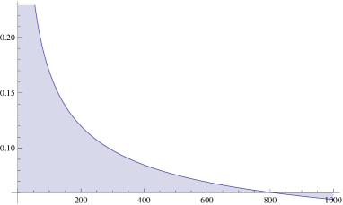
Figure 1: The evolution of $\Phi$, for $r_{G}=2.99~{}km$.

Adding Eq. (2) and Eq. (3), to get $\Phi^{\prime}=-\Lambda^{\prime}$ then substituting this value in Eq. (4). Thus this system can be reduced to

$$re^{2\Phi}=r\pm a,$$ (5)

where $a$ is constat.

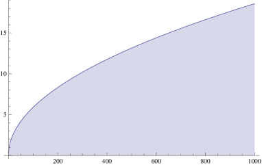
Figure 2: The evolution of $\Lambda$, with different $r_{G}=2.99~{}km$.

3 Some Special Cases

Here we examine the existence of some special points by considering it’s geometry and observe their importance in different forms of spherical metric.

$\bullet$ Case I: When $r\rightarrow\infty$, very large enough, in the case of accelerating universe, $e^{2\Phi}=1$,     $e^{2\Lambda}=1$, then we obtain the metric

$$ds^{2}=-dt^{2}+dr^{2}+r^{2}[d\theta^{2}+sin^{2}\theta d\phi^{2}],$$ (6)

this describes a Minkowskian (spacetime)line element outside matter distribution.
$\bullet$ Case II: When $a=r_{G}$ gravitational radius of the body. Thus the metric is reduced to

$$ds^{2}=-(1-{{r_{G}}\over{r}})dt^{2}+(1-{{r_{G}}\over{r}})^{-1}dr^{2}+r^{2}[d\theta^{2}+sin^{2}\theta d\phi^{2}],$$

is called Schwarzschild line element.
$\bullet$ Case III: When $a=r=r_{G}$, then $g_{tt}=0$ and $g_{rr}=\infty$. Thus it should be noted that Schwarzschild metric become singular at that point. However, for most of the observable bodied in the universe the gravitational radius lies well inside them. For example in the case of Sun the value of $r_{G}=2.9km$ and for our Earth its value is $0.88cm$.
$\bullet$ Case IV: At $a=r$, we have $e^{2\Phi}=1+{{a}\over{r}}$, then metric reduces to the form

$$ds^{2}=-2dt^{2}+{{1}\over{2}}dr^{2}+r^{2}(d\theta^{2}+sin^{2}\theta d\phi^{2})$$ (7)

this describes a very special metric of the Universe and its properties are not yet discussed in this paper.

4 Solutions of the Einstein Equation with Sources

To find some spherical space times that are not singular along the central axis. We need to solve Einstein equations, where stress energy tensor $T$ has nonzero components, first we have to find some basic quantities and tensors encountered in general relativity. For this we find the Ricci scalar, $R$, the Einstein tensor, $G_{\mu\nu}$, and the stress energy tensor, $T_{\mu\nu}$, for the spherically symmetric metric given in (1)
Ricci scalar:

$$R=e^{-2\Lambda}\left[-2\Phi^{\prime\prime}-2{\Phi^{\prime}}^{2}+2{\Lambda^{\prime}}{\Phi^{\prime}}-4\frac{\Phi^{\prime}}{r}+4\frac{\Lambda^{\prime}}{r}-\frac{2}{r^{2}}\right]+{{2}\over{r^{2}}}$$ (8)

Nonzero Einstein Tensor Components are:

$$G_{tt} = e^{2(\Phi-\Lambda)}(\frac{2\Lambda^{\prime}}{r}-\frac{1}{r^{2}})+{{1}\over{r^{2}}}e^{2\Phi}$$

$$G_{rr} = \frac{2\Phi^{\prime}}{r}+\frac{1}{r^{2}}-{{1}\over{r^{2}}}e^{2\Lambda}$$

$$G_{\theta\theta} = e^{-2\Lambda}{r^{2}}\left[\Phi^{\prime\prime}+{\Phi^{\prime}}^{2}-{\Lambda^{\prime}}{\Phi^{\prime}}+\frac{\Phi^{\prime}}{r}-\frac{\Lambda^{\prime}}{r}\right]$$

$$G_{\phi\phi}=e^{-2\Lambda}{r^{2}}sin^{2}{\theta}\left[\Phi^{\prime\prime}+{\Phi^{\prime}}^{2}-{\Lambda^{\prime}}{\Phi^{\prime}}+\frac{\Phi^{\prime}}{r}-\frac{\Lambda^{\prime}}{r}\right].$$ (9)

The stress energy tensor components are defined by $T_{{r}}^{r}=p_{r}$ and $T_{rr}=p_{r}e^{2\Lambda}$, similarly the remaining pressure components are defined, similarly also we have $T_{{t}}^{t}=-\rho$
Nonzero Stress Tensor Components are:

$$T_{tt}=\rho{e^{2\Phi}}$$

$$T_{rr}=p_{r}{e^{2\Lambda}}$$

$$T_{\theta\theta}=p_{\theta}{r^{2}}$$

$$T_{\phi\phi}=p_{\phi}{r^{2}}sin^{2}{\theta}$$ (10)

In General Relativity (GR), the symmetric stress-energy tensor acts as the source of spacetime curvature. While dealing with the curved spacetime due to the existence of matter, the Riemann tensor plays a vital role as seen in GR. One very important equation in this subject is the Einstein field equation, a tensorial equation which takes the form $G_{\mu\nu}=8\pi T_{\mu\nu}$, $G_{\mu\nu}$ is an Einstein’s tensor which is symmetric and vanishes when spacetime is flat, $T_{\mu\nu}$ is the so-called energy-momentum tensor which can be thought of as a source for the gravitational field. It is a divergenceless tensor due to the conservation of energy, namely $\nabla^{\mu}T_{{\mu\nu}}=0$. The proportionality constant is $8\pi$ since we use the natural units, otherwise it would be $\frac{8\pi G}{c^{4}}$.

Mathematically, the Einstein’s tensor is given by $G_{\mu\nu}=R_{\mu\nu}-\frac{1}{2}g_{\mu\nu}R$, where Ricci tensor is a contraction of the Riemann tensor $(R_{\mu\nu}=R_{{\gamma}}^{\mu\gamma\nu})$, and R is a curvature scalar obtained from the Ricci tensor, hence also called Ricci scalar. The full form of the Einstein equation has an extra term owing to the Cosmological constant $(\Lambda^{*})$, which has been found recently to be an extremely tiny number but non-zero. It reads $G_{\mu\nu}-{\Lambda^{*}}g_{\mu\nu}=8\pi T_{\mu\nu}$ The significance of the cosmological constant is involved mostly in the context of cosmology in which one studies the fate of the universe (for example see Ref. [12]), from $T^{\mu\nu}_{;\nu}=0$ we have

$$0=\frac{\partial p_{r}}{\partial r}+p_{r}(\Phi^{\prime}+\frac{2}{r})+\rho\Phi^{\prime}-\frac{p_{\theta}}{r}-\frac{p_{\phi}}{r}$$ (11)

$$4\pi(\rho+p_{r}+p_{\theta}+p_{\phi})e^{2\Lambda}=\Phi^{\prime\prime}+{\Phi^{\prime}}^{2}-{\Lambda^{\prime}}{\Phi^{\prime}}+\frac{2\Phi^{\prime}}{r}$$ (12)

$$4\pi(\rho+p_{r}-p_{\theta}-p_{\phi})e^{2\Lambda}=-\Phi^{\prime\prime}-{\Phi^{\prime}}^{2}+{\Lambda^{\prime}}{\Phi^{\prime}}+\frac{2\Lambda^{\prime}}{r}$$ (13)

$$4\pi(\rho-p_{r}+p_{\theta}-p_{\phi})e^{2\Lambda}=\frac{\Lambda^{\prime}}{r}-\frac{\Phi^{\prime}}{r}-\frac{1}{r^{2}}+{{1}\over{r^{2}}}e^{2\Lambda}$$ (14)

$$4\pi(\rho-p_{r}-p_{\theta}+p_{\phi})e^{2\Lambda}=\frac{\Lambda^{\prime}}{r}-\frac{\Phi^{\prime}}{r}-\frac{1}{r^{2}}+{{1}\over{r^{2}}}e^{2\Lambda}$$ (15)

Now adding equation (12) and (13) then subtracting equation (15). This gives

$$4\pi(\rho+3p_{r}+p_{\theta}-p_{\phi})e^{2\Lambda}=3\frac{\Phi^{\prime}}{r}+\frac{\Lambda^{\prime}}{r}+\frac{1}{r^{2}}-{{1}\over{r^{2}}}e^{2\Lambda}$$ (16)

Now we add and subtract equation (14) in equation (16) and get simultaneously results,

$$4\pi(2\rho+2p_{r}+2p_{\theta}-2p_{\phi})e^{2\Lambda}=2\frac{\Phi^{\prime}}{r}+2\frac{\Lambda^{\prime}}{r}$$ (17)

$$4\pi(4p_{r})e^{2\Lambda}=4\frac{\Phi^{\prime}}{r}+\frac{2}{r^{2}}-{{2}\over{r^{2}}}e^{2\Lambda}$$ (18)

Here we have a system of differential equations namely Eqs. (11), (12), (14) and (15) can be solved for $p_{r}\;\;,p_{\theta}\;\;,p_{\phi}\;\;,\Phi\;\;and\;\;\Lambda$. Further Eq. (18) which contains only first order derivative of the unknown function, posses an additional constraint. Thus the above system of five equations is second order in $\Phi$ and first order in $\Lambda$ and $p_{r}$.
By taking derivative of equation (18) with respect to $r$ and putting values of equations (11), (12), (15) and (17) to substitute for $p^{\prime}_{r}$, $\Lambda^{\prime}$ and $\Phi^{\prime\prime}$ resulting a relation which reduces $0=0$ thus equation (18) would must hold for all $r$ if it holds at any value of $r$ .

5 A Solution with $\rho=-p_{\phi}\;\;,p_{r}=p_{\theta}=0$

The generic solution of these differential equations for arbitrary values of our unknown $\rho,\;\;p_{r},\;\;p_{\theta}\;\;and\;\;p_{\phi}$ is much more difficult and out of scope of this paper. For simplicity of finding the solution of equation, one can take the value $\rho=-p_{\phi}$ and the remaining pressure components are zero. Thus from equations (11), (12), (14), (15), (17) and (18) respectively, someone can get

$$0=\rho\left(\Phi^{\prime}+\frac{1}{r}\right)$$ (19)

$$0=\Phi^{\prime\prime}+{\Phi^{\prime}}^{2}-{\Lambda^{\prime}}{\Phi^{\prime}}+\frac{2\Phi^{\prime}}{r}$$ (20)

$$4\pi(2\rho)e^{2\Lambda}=\frac{\Lambda^{\prime}}{r}-\frac{\Phi^{\prime}}{r}-\frac{1}{r^{2}}+{{1}\over{r^{2}}}e^{2\Lambda}$$ (21)

$$0=\frac{\Lambda^{\prime}}{r}-\frac{\Phi^{\prime}}{r}-\frac{1}{r^{2}}+{{1}\over{r^{2}}}e^{2\Lambda}$$ (22)

$$4\pi(2\rho)e^{2\Lambda}=\frac{\Lambda^{\prime}}{r}+\frac{\Phi^{\prime}}{r}$$ (23)

and

$$0=2\frac{\Phi^{\prime}}{r}+\frac{1}{r^{2}}-{{1}\over{r^{2}}}e^{\Lambda}$$ (24)

From Eq. (19), we get $\Phi=\ln[{1/r}]$ and with the help of Eq. (19), we obtain from Eq. (21) $\Lambda^{\prime}={{(8\pi\rho r^{2}-1)}\over{r}}e^{2\Lambda},$ thus the metric of the solution is

$$ds^{2}=-r^{-2}dt^{2}+e^{2\Lambda}dr^{2}+r^{2}d\theta^{2}+r^{2}sin^{2}\theta d\phi^{2}.$$ (25)

If we take the value of $\rho=1/{8\pi r^{2}_{0}}$, which is well known result in literature, then our final solution becomes

$$ds^{2}=-r^{-2}dt^{2}+[r^{2}_{0}/(r^{2}_{0}ln{r^{2}}-r^{2})]dr^{2}+r^{2}d\theta^{2}+r^{2}sin^{2}\theta d\phi^{2}.$$ (26)

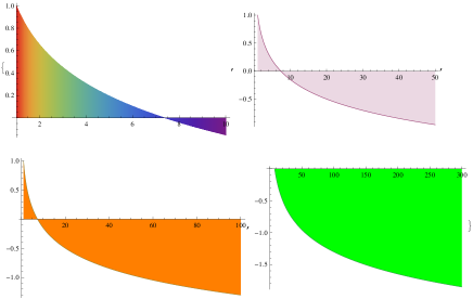
Figure 3: The evolution of $\Phi$, with different panels, representation of Universe.

6 Discussion

Spherical symmetry in general relativity turns out to be similar to Cylindrical symmetry in many of its behavior but very different in other actions.. We have presented analytical solution with spherical symmetric approach with more conventional interior sources and more general exterior geometry. However the construction of a variety of solutions presented here illustrates several informative points about metric of the Universe. On the basis of information we would like to decide the ultimate fate of the Universe.
Furthermore, the choice of gauge (coordinate system) is always a major issue in relativity; the same space-time can look quite different in different gauges, and how (and whether) to choose a standard gauge or “normal form” for a given problem is not always understandable. There are many acceptable ways to fix the gauge, and we have taken pains to describe them all and how they are related. Even after a definition of radial coordinate has been selected, further steps to a normal form can be taken by linear rescaling of the coordinates. The structure of the Einstein equation system is nontrivial. There is one more equation than one might naively expect. The extra equation serves as a constraint on the data. For the spherical vacuum solutions this constraint is a simple algebraic relation among the parameters.
Finally, we observed some surprising ambiguities of interpretation. For the evolution of $\Phi$ (see figure 1) an increasing radius, feasible region is disappear from actual frame for fixing the value of $r_{G}=2.99~{}km$, but in the case of evolution of $\Lambda$ (see figure 2 ) shows increasing behavior due to increase of $r$ in the given metric. However, we observed that when $r$ is large enough, then actual region in upper half is decreasing, ratio of two reign is decreasing. It means that ratio is directly proportional to $r$, therefore, we see from (figure 3) that in below left panel upper region will be completely disappear, which is the consistency of our theoretical results.
Furthermore, numerical solution with different parameters of the metric still need special attention for future work. In future work, we intend to investigate the compatibility of the conformal spherical symmetry with homogeneity, and also with the kinematical quantities.

7 Acknowledgment

The author would like to thanks Dr. Muhammad Nizamuddin for providing the facilities to carry out the research work and we thank Yun-Song Piao for useful suggestion.

References

• [1] H. Stephani, D. Kramer, M. MacCallum, C. Hoenselaers and E. Herlt, Exact solutions to Einstein s field equations (2003) (Cambridge:Cambridge University Press)
• [2] H. Weyl, Ann. Phys., Lpz.(1917) 54 117
• [3] T. Levi-Civita, Atti Acc. Lincei Rend. 28 (1919) 101
• [4] L. Marder, Proc. R. Soc. Lond. A 244 (1958) 524
• [5] J.R. Gott, Ap. J. 288 (1985) 422
• [6] W.A. Hiscock, Phys. Rev. D 31(1985) 3288
• [7] D. Garfinkle, Phys. Rev. D 32 (1985) 1323
• [8] B.F. Schutz, A First Course in General Relativity (2009) (Cambridge:Cambridge University Press) p 135, 159, 164, 256
• [9] M. Carmeli, Claasical fields: General Relativity and Gauge Theory (1982) John Wiley and sonsp 23, 33, 45, 51, 67
• [10] C.S. Trendafilova and S.A. Fulling, Eur. J. Phys. 32 (2011) 1663.
• [11] C. Huneau, Constraint equations for vacuum Einstein equations with a S1 symmetry ( arXiv:1302.1473 [math.AP]).
• [12] N. Pidokrajt, Black Hole Thermodynamics (2003)(Thesis) (Department of Physics, Stock-holm University)