Controlling the Polarity of the Transient Ferromagnetic-Like State in Ferrimagnets

Abstract

It was recently observed that the two antiferromagnetically coupled sublattices of a rare earth-transition metal ferrimagnet can temporarily align ferromagnetically during femtosecond laser heating, but always with the transition metal aligning in the rare earth direction. This behavior has been attributed to the slower magnetization dynamics of the rare earth sublattice. The aim of this work was to assess how the difference in the speed of the transition metal and rare earth dynamics affects the formation of the transient ferromagnetic-like state and consequently controls its formation. Our investigation was performed using extensive atomistic spin simulations and analytic micromagnetic theory of ferrimagnets, with analysis of a large area of parameter space such as initial temperature, Gd concentration and laser fluence. Surprisingly, we found that at high temperatures, close to the Curie point, the rare earth dynamics become faster than those of the transition metal. Subsequently we show that the transient state can be formed with the opposite polarity, where the rare earth aligns in the transition metal direction. Our findings shed light on the complex behavior of this class of ferrimagnetic materials and highlight an important feature which must be considered, or even exploited, if these materials are to be used in ultrafast magnetic devices.

I Introduction

Unexpected states in solid state physics attract a lot of attention from a fundamental point of view. A recent example is the transient ferromagnetic-like state (TFLS) in ferrimagnetic GdFeCo. RaduNature2011 ; OstlerNatureComm2012 ; KirilyukPhysRep2013 ; LeGuyaderAPL12 Element specific femtosecond resolution X-ray magnetic circular dichroismSiegmannBook2006 has shown that following the application of a femtosecond laser pulse, the FeCo sublattice magnetization points in the same direction as the Gd sublattice magnetization. This transient state lasts for just a few picoseconds, but the alignment against the strong antiferromagnetic coupling between the sublattices is very stable, even against large opposing magnetic fields.OstlerNatureComm2012 More recent work has shown a similar behavior in TbFe alloys, KhorsandPRL13 suggesting this state may exist in a whole class of materials. In this paper we study the TFLS in more depth, especially how the difference in relaxation times of the transition metal (TM) and rare earth (RE) sublattices leads to its formation. We find that the TFLS can also form with the alignment of the rare earth towards the transition metal sublattice, the opposite polarity to that which has been found previously. This change in polarity comes about due to a difference in the temperature dependence of the characteristic relaxation times of the two sublattices, leading to a crossover behavior, making the rare earth response faster than that of the transition metal. This is a stark contrast to the commonly proposed relation that the relaxation time of a magnetic species is proportional to the ratio of its atomic magnetic moment $\mu_{0}$ and the intrinsic Gilbert damping $\lambda$, KazantsevaEPL2008 ; MentinkPRL2012 a relation which would lead to the false conclusion that the rare earth is always slower that the transition metal. Understanding this difference is important if these materials are to be used for ultrafast magnetic devices, especially where large, dynamic temperature ranges are used.

Several theoretical descriptions have been proposed to describe the physical mechanisms underlying the TFLS. MentinkPRL2012 ; KoopmansPRB13 ; AtxitiaPRB2012 ; JoeSREP2013 All of them suggest that the TFLS is formed by an exchange of angular momentum between TM and RE magnetic lattices driven by the antiferromagnetic exchange coupling. The magnetization transfer leads to the TFLS in a non-equilibrium situation between both magnetic sublattices. The heating produced by the laser pulse causes the TM magnetization to nearly vanish, while that of the RE remains finite. Such a behavior is only possible if the demagnetization times (energy input absorption rate) of the two sublattices are sufficiently different. Therefore it is necessary to establish a theoretical approach to estimate the relationship between the relaxation times of each sublattice in ferrimagnets which would allow the engineering of generic ferrimagnetic materials, such as synthetic ferrimagnets, EvansArxiv2013 where this phenomenon could occur.

In pure ferromagnets the ratio between the magnetic moment and the Curie temperature, $\mu_{0}/T_{c}$ (or more precisely AtxitiaQ $\mu_{0}/\lambda T_{c}$) has been shown to be a good approximation of the speed of demagnetization, allowing one to classify ferromagnetic materials into two types, fast and slow. KoopmansNatMat10 Using this simplistic argument in TM-RE alloys such as TbFe, KhorsandPRL13 TbCo,AlebrandAPL12 or GdFeCo OstlerNatureComm2012 and assuming a shared $T_{c}$, OstlerPRB2011 transition metal demagnetization times are approximately $\mu_{{\text{\tiny{RE}}}}/\mu_{{\text{\tiny{TM}}}}\approx 4-5$ times faster than those of the rare earth. This simple relationship has been shown to work well for temperatures far below the Curie point. KoopmansNatMat10 This reasoning restricts the formation of the TFLS to a polarity where the TM magnetization will always reverse to align in the RE direction.

The importance of the initial temperature ($T_{0}$) on the demagnetization behavior was shown in recent experiments on ferromagnetic Ni thin films where the initial temperature before laser heating was systematically varied.KoopmansPRX2012 It was demonstrated that as $T_{0}$ increases the observed fast demagnetization becomes a well-defined two step process. Namely, an initial sub-ps demagnetization followed by a much slower demagnetization process of the order of several ps. Similar results where also obtained in Ni AtxitiaPRB10 and FePt thin filmsMendilarxiv2013 keeping the initial temperature fixed but increasing the laser fluency, and thus reaching higher temperatures. The observed slowing down of the magnetization response was associated to the increasing role played by the spin fluctuations for temperatures approaching $T_{c}$. In rare earth-transition metal alloys, similar experiments have been recently performed in situations where, although the initial temperature was varied, it did not approach $T_{c}$ closely enough to obtain clear evidence of the demagnetization behavior.MedapalliEPJB2013 ; LopezfloresArxiv2013 From general phase transition theory RushbrookeBook one may expect that approaching $T_{c}$, both sublattices would experience critical slowing down. However it is not clear if the critical slowing down is equal for both sublattices and whether the non-equivalence criterion, $\mu_{{\text{\tiny{RE}}}}/\mu_{{\text{\tiny{TM}}}}$, still holds close to $T_{c}$. To answer these questions, we theoretically investigate the dynamical response of TM-RE alloys to femtosecond heating as a function of the initial temperature and the TM-RE composition, using the prototypical example of GdFeCo.

We use the Landau-Lifshitz-Bloch (LLB) equation for multi-sublattice magnets AtxitiaPRB2012LLBferrim to provide the quantitative calculation of the magnetization relaxation times for each lattice, including those close to $T_{c}$ in GdFeCo. These calculations are complemented by large scale computer simulations based on the stochastic Landau-Lifshitz-Gilbert (LLG) equation of motion for an atomistic spin model. These simulations confirm the proposed scenario for the formation of the TFLS based on the angular momentum transfer between the two sublattices.JoeSREP2013 ; AtxitiaPRB2012 Importantly, we derive theoretically the necessary conditions for the formation of the TFLS with a reversed polarity and confirm the criteria by means of atomistic spin dynamic simulations. The paper is organized as follows. We first outline the basis of the atomistic spin model followed by a consideration of the sublattice relaxation times based on the ferrimagnetic Landau-Lifshitz-Bloch equation and importantly link this to the equilibrium magnetization curves. This leads to a criterion for equivalent sublattice relaxation times, which defines a region separating opposite polarities of TFLS; a result supported by the large-scale atomistic model simulations.

II Theoretical description of ultrafast magnetization dynamics in two-sublattice ferrimagnets.

II.1 Atomistic spin model for GdFeCo alloys

The energetics of the ferrimagnetic system are described by the classical Heisenberg Hamiltonian

$$\mathcal{H}=-\tfrac{1}{2}\sum_{\langle ij\rangle}J_{ij}\mathbf{S}_{i}\cdot\mathbf{S}_{j}-\sum_{i}d_{z,i}(S_{z,i})^{2}$$ (1)

where $\langle ij\rangle$ indicates that the sum is limited to nearest neighbor pairs with $\left|\mathbf{S}_{i}\right|=\bm{\mu}_{i}/\mu_{i}$, $\bm{\mu}_{i}$ representing the atomic magnetic moment. We use a random lattice model to represent the amorphous property of GdFeCo (see Refs. OstlerNatureComm2012, and JoeSREP2013, ). We assume a simple cubic lattice of FeCo moments and randomly substitute sites with Gd moments until the desired Gd concentration, $x$, is achieved, giving a system of Gd_x(FeCo)_1-x. The FeCo sublattice has a moment $\mu_{{\text{\tiny{FeCo}}}}=2.217\mu_{\mathrm{B}}$ representing the $3d$ itinerant electrons. BozorthBook2003 The use of a common sublattice to model FeCo is justified since the Fe and Co moments are delocalized in nature and are parallel to one another up to the Curie temperature. Moreover, the amount of Co used in the GdFeCo alloys studied in experiments is small. In our model the Gd sublattice is attributed a moment of $\mu_{{\text{\tiny{Gd}}}}=7.63\mu_{\mathrm{B}}$ which takes into account the contribution of the half-filled localized $4f$ shell ($7\mu_{B}$) and itinerant $5d$ electrons spin ($0.63\mu_{B}$)JensenBook1991 ($\mu_{\mathrm{B}}$ is the Bohr magneton in both cases). The values of exchange energy, $J_{ij}$, we use give good agreement to the experimental data of GdFeCo for the Curie temperature, $T_{c}$, and compensation point, $T_{M}$, where $M_{\mathrm{FeCo}}=M_{\mathrm{Gd}}$. Here, $M_{\mathrm{FeCo}}(T)=(1-x)\mu_{{\text{\tiny{FeCo}}}}\langle S_{\mathrm{FeCo}}\rangle(T)$ and $M_{\mathrm{Gd}}(T)=x\mu_{{\text{\tiny{Gd}}}}\langle S_{\mathrm{Gd}}\rangle(T)$ are the macroscopic magnetization of the FeCo and Gd sublattices, respectively.

The thermodynamic average the spin fluctuations of each sublattice, $\langle S_{\mathrm{Gd}}\rangle(T)$ and $\langle S_{\mathrm{FeCo}}\rangle(T)$, can be calculated using either the mean field approximation or using computational models. OstlerPRB2011 In the atomistic spin model we will use computer simulations with the values for exchange energy $J_{{\text{\tiny{RR}}}}=2.3970\times 10^{-21}$J and $J_{{\text{\tiny{TT}}}}=1.0067\times 10^{-20}$J (ferromagnetic coupling) and $J_{{\text{\tiny{RT}}}}=-2.7805\times 10^{-21}$J (antiferromagnetic coupling). Typical Gd concentrations used in recent experiments of ultrafast dynamics range from $10$ to $30\%$. KirilyukPhysRep2013 Hence, these alloys behave as an “effective” ferromagnet, FeCo, defined mainly by the value of the intra-lattice exchange integral, $J_{{\text{\tiny{TT}}}}$, and the Gd spins whose dynamics are mainly defined by the antiferromagnetic coupling to the FeCo spins, defined by the exchange integral $J_{{\text{\tiny{TR}}}}$. The effect of Gd-Gd exchange interactions in these Gd concentrations ($10-30\%$) is relatively small in comparison to other exchange interactions present in the system. We note that although in this work we are studying GdFeCo alloys in particular, the model described above is general and can be adapted to any other rare earth - transition metal alloy. The second term in the Hamiltonian represents a uniaxial anisotropy energy which is consistent with the observed out of plane magnetization of these alloys. We use a value of $d_{z}=8.07246\times 10^{-24}$ J for both FeCo and Gd sublattices.OstlerPRB2011

The dynamics of the atomistic spins interacting with a heat bath are described by the coupled stochastic Landau-Lifshitz-Gilbert (LLG) equations of motion

$$\frac{\mathrm{d}\mathbf{S}_{i}}{\mathrm{d}t}=-\frac{\gamma_{i}}{(1+\lambda_{i}^{2})}\left[\mathbf{S}_{i}\times\mathbf{H}_{i,\mathrm{eff}}+\lambda_{i}\mathbf{S}_{i}\times(\mathbf{S}_{i}\times\mathbf{H}_{i,\mathrm{eff}})\right]$$ (2)

where $\gamma_{i}$ is the gyromagnetic ratio, $\lambda_{i}$ is the coupling strength of the spin $i$ to the heat bath and the effective field of a spin on lattice site $i$ is

$$\mathbf{H}_{i,\mathrm{eff}}=-\frac{1}{\mu_{i}}\frac{\partial\mathcal{H}}{\partial\mathbf{S}_{i}}+\bm{\zeta}_{i}.$$ (3)

The stochastic fields, $\bm{\zeta}_{i}$, represent the thermal fluctuations. Although one can in principle consider colored thermal noise, AtxitiaPRL2009 here we assume that it is uncorrelated in space and time, i.e. the white noise approximation. The first and second moments of the bath variable are written as:

$$\langle\zeta^{k}_{i}\rangle=0,\quad\langle\zeta^{k}_{i}(t)\zeta^{l}_{j}(t^{\prime})\rangle=2\lambda_{i}\frac{\mu_{i}}{\gamma_{i}}k_{\mathrm{B}}T\delta_{ij}\delta_{kl}\delta(t-t^{\prime}),$$ (4)

where $i,j$ denotes lattice sites and $k,l$ are the Cartesian components, $k_{B}$ is the Boltzmann constant, and $T$ is the heat-bath temperature. We couple the spin system to a heat bath representing the electronic system and defined by the temperature $T_{e}$. This acts as the origin of the spin-flip processes and is where energy enters the system from the laser heating. KazantsevaPRB2008 The coupling constant $\lambda_{i}$ essentially represents the energy transfer rate between the spin and heat bath. Here each sublattice is separately coupled to the same heat bath, although they could be coupled to different heath baths, such as electron and phonon heat baths as shown in Ref. WienholdtPRB2013, or the same sublattice can be coupled simultaneously to the two baths. SultanPRB2012 As a consequence of the different magnetization response of each sublattice, given by the intrinsic parameters, one sublattice can heat faster (“hot”) than the other (“cold”). The absorbed energy is afterwards dissipated in both the heat bath (fluctuation-dissipation) and to the other sublattice (and eventually to the heat bath) through the atomic scale exchange coupling. EllisPRB2012 The transient ferromagnetic like state in GdFeCo is formed under non-equilibrium situations where the latter mechanism dominates. AtxitiaPRB2012

Atomistic spin models of this type have become a de facto tool in the investigation of ultrafast magnetism due to their good quantitative description of the temperature dependent magnetic properties, as well as the timescales of dynamical phenomenon such as the TFLS. In principle one can include many complexities into such a model, for example different values of $\gamma_{i}$ and $\lambda_{i}$. Such scenarios may be closer to the physical reality, however to clearly explain the most basic relationships behind the dynamics which cause the formation of the TFLS we assume $\gamma_{\mathrm{FeCo}}=\gamma_{\mathrm{Gd}}=\gamma_{e}$ and $\lambda_{\mathrm{FeCo}}=\lambda_{\mathrm{Gd}}=0.01$. These values are the same as those used in previous works and describe well the ultrafast demagnetization time scales found experimentally. OstlerNatureComm2012

II.2 Formation of the transient ferromagnetic like state

The role of the magnetization compensation point in the laser induced magnetization switching and the TFLS formation is still a subject of controversy in the literature. StanciuPRL2007 ; MekomenPRL2011 ; WienholdtPRL12 ; AlebrandPRB2012 ; HassdenteufelAdvanceMaterials13 ; SchlickeiserPRB2012 ; JoeSREP2013 Recently we showed that a minimum amount of laser energy input of the order of the energy gap between the two ferrimagnetic modes, i.e. $\hbar\Delta\omega\sim\hbar\omega_{\mathrm{ex}}\sim J_{{\text{\tiny{RT}}}}\left(M_{\mathrm{FeCo}}(T_{0})-M_{\mathrm{Gd}}(T_{0})\right)$, is required for the formation of the TFLS,JoeSREP2013 where $\omega_{\mathrm{ex}}$ is the frequency of the so-called antiferromagnetic coherent exchange mode. The disordered nature of the GdFeCo spin lattice leads an effect that the most efficient energy transfer (the smallest energy gap) does not correspond exactly to the coherent mode with $k=0$ but to non-zero $k$ value, related to the characteristic length of the Gd spins cluster size.JoeSREP2013

This slightly shifts the minimum energy for the TFLS formation with respect to the magnetization compensation point, where $M_{\mathrm{FeCo}}(T_{0})\approx M_{\mathrm{Gd}}(T_{0})$ but the minimum energy still lies close to it. The condition for the minimum energy gap can be fulfilled in two temperature regions (i) close to the $T_{M}$ where $M_{\mathrm{FeCo}}(T_{M})\approx M_{\mathrm{Gd}}(T_{M})$, (with $M_{\mathrm{FeCo}}(T_{M})\neq 0,M_{\mathrm{Gd}}(T_{M})\neq 0$), and (ii) approaching the Curie temperature $T_{c}$, where both $M_{\mathrm{FeCo}}(T_{M})$ and $M_{\mathrm{Gd}}(T_{M})$ are close to zero. The temperature dependence of the ferrimagnetic exchange modes depends on the concentration of Gd ($x$), the initial temperature ($T_{0}$) and the inter-lattice exchange coupling ($J_{{\text{\tiny{RT}}}}$). SchlickeiserPRB2012 Among these parameters $x$ and $T_{0}$ can be changed experimentally however $J_{{\text{\tiny{RT}}}}$ is very difficult to change in a GdFeCo alloy. We therefore focus on the fundamental properties of the TFLS formation by varying the concentration and initial temperature.

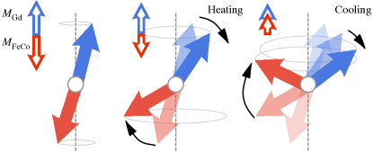
Figure 1: Schematic description of the transition into the transient ferromagnetic-like state (TFLS) with rare earth (RE) polarity. Initially, at equilibrium, there is little excitation of high energy antiferromagnetic exchange spin oscillations. During the heating phase these are excited and the TFLS is formed with RE polarity since the RE dynamics are faster.

Figure 1 shows a schematic representation of the transient ferromagnetic like state formation. As explained in detail in Ref. JoeSREP2013, , three well defined regions can be distinguished (i) at equilibrium before laser heating, the thermal excitation of the modes does not lead to any net spin transfer between sublattices, (ii) during laser heating, the spin wave modes of the system are excited out of equilibrium, leading to an efficient transfer of spin angular momentum between sublattices. JoeSREP2013 (iii) This process results in a precessional reversal path for the magnetization at the nanoscale AtxitiaPRB2012 . Around $T_{M}$ the energy efficiency of this mechanism is large since the relevant modes are lower in energy ($\hbar\omega_{\textrm{ex}}(T_{M})\approx 0$) than when the system is far from $T_{M}$. JoeSREP2013 Nevertheless, this does not restrict the appearance of the TFLS to the existence of any compensation point. Indeed the TFLS has been shown above the compensation point both in spin models and experimentally. OstlerNatureComm2012

Apart from the excitation of those modes, before the TFLS can form, a full macroscopic demagnetization of the magnetic sublattice which switches (hot) is needed, OstlerNatureComm2012 whereas the other remains finite (cold). Hence, the heating produced by the laser pulse into one of the sublattices should have the same time scale as the magnetization relaxation time $\tau_{\nu,\|}$, with $\nu=$RE,TM. Thus, the estimation of $\tau_{\nu,\|}$ is of fundamental importance.

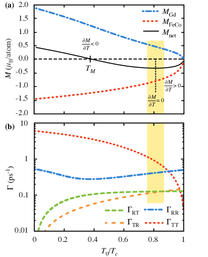
Figure 2: (a) Equilibrium magnetization of each sublattice as a function of reduced temperature $T_{0}/T_{c}$ ($T_{c}=800$ K). The yellow shaded region corresponds to $\partial M_{\textrm{net}}/\partial T=0$ and separates two regions, $\partial M_{\mathrm{FeCo}}/\partial T<\partial M_{\mathrm{Gd}}/\partial T$ and $\partial M_{\mathrm{Gd}}/\partial T>\partial M_{\mathrm{FeCo}}/\partial T$. (b) Relaxation rate parameters defining the Landau-Lifshitz-Bloch dynamical equation as a function of $T_{0}/T_{c}$.

II.3 Estimation of the temperature dependent magnetization relaxation time in ferromagnets

The demagnetization behavior of even simple ferromagnets, after a femtosecond timescale laser pulse, is still a subject of intensive research. MannPRX2012 ; WietstrukPRL2011 ; BattiatoPRL2010 ; SchellekensPRL2013 ; AtxitiaQ ; ManchonPRB2012 ; MuellerPRL2013 In ferrimagnets, there is a large interest on demagnetization rates of each species, following the use of X-ray magnetic circular dichroism SiegmannBook2006 to monitor the sub-picosecond dynamics of each sublattice magnetization individually. KirilyukPhysRep2013 Thermal effects dominate the magnetization dynamics during the heating produced by the laser. On this basis recent works KazantsevaEPL2008 ; MentinkPRL2012 suggested that the typical demagnetization time of the sublattice $\nu$ is given by $\tau_{\nu}\sim\gamma_{\nu}\mu_{\nu}/(\lambda_{\nu}k_{\mathrm{B}}T_{e})$, where $T_{e}$ refers to the dynamical electron temperature. This estimate is based on the assumption that the magnetic system behaves as a paramagnet before or instantaneously after the application of the heating. Effectively this assumes that the dynamics is completely dominated by temperature and all spin correlations are lost, thus this time scale takes no account of the magnetic interactions. This assumption is extremely hard to justify in light of recent theories which suggest the spin correlations play an important role in forming the TFLS.JoeSREP2013 Nevertheless, for GdFeCo alloys, it has been found to give a good estimate of the relationship between the demagnetization times of FeCo and Gd sublattice when compared to experimental observations where $\tau_{{\text{\tiny{Gd}}}}/\tau_{{\text{\tiny{FeCo}}}}\approx\mu_{{\text{\tiny{Gd}}}}/\mu_{{\text{\tiny{FeCo}}}}\approx 3.5$ (a $\lambda_{{\text{\tiny{Gd}}}}=\lambda_{{\text{\tiny{FeCo}}}}$ were assumed). RaduNature2011 This coincidence has caused some confusion and restricts research on this new phenomenon to materials with very different atomic magnetic moments.

More sophisticated approaches such as the Landau-Lifshitz-Bloch (LLB) AtxitiaPRB10 ; AtxitiaQ and microscopic three temperature model (M3TM) KoopmansNatMat10 models take into account the spin exchange interactions within the mean field approximation. The M3TM model also within the MFA (Weiss) shows that the timescale is essentially defined by $\mu_{0}/T_{c}$. Within the LLB model a similar estimate can been found.AtxitiaQ In particular, for ferromagnets, the relaxation time has been shown to be defined as $\tau_{\|}\sim\widetilde{\chi}_{\|}(T)/\lambda$, where $\widetilde{\chi}_{\|}=(\partial m/\partial H)_{H\rightarrow\infty}$ is the longitudinal susceptibility and $m$ is the thermally averaged spin polarization. This depends on: (i) the particular dissipation mechanism represented by the coupling parameter $\lambda$, and (ii) the longitudinal susceptibility $\widetilde{\chi}_{\|}(T)$. In the LLB model $\lambda$ is related to the spin-flip scattering probabilities, and taken as a parameter GaraninPhysicaA91 ; UnpublishedPablo while within the M3TM model it is related to electron-phonon Elliot-Yafet scattering mechanism. SchellekensPRL2013

In the MFA the longitudinal susceptibility can be calculated using the equilibrium magnetization curve given by the Curie-Weiss equation $m=\mathcal{L}(mJ_{0}/k_{\mathrm{B}}T)$, where $\mathcal{L}$ stands for the Langevin function in the classical case, $\mathcal{L}(x)=\coth(x)-1/x$ and $J_{0}=\sum_{j}J_{0j}=3k_{B}T_{c}$. It reads

$$\widetilde{\chi}_{\|}(T)=\frac{\mu_{0}}{J_{0}}\frac{\beta J_{0}\mathcal{L}^{\prime}}{1-\beta J_{0}\mathcal{L}^{\prime}}\approx\left\{\begin{array}[]{ccc}c_{0}\frac{\mu_{0}}{T_{c}},&&T\ll T_{c}\\ &&\\ \frac{\mu_{0}}{2}\frac{T_{c}}{T-T_{c}},&&T\lesssim T_{c}\end{array}\right.$$ (5)

where $\mathcal{L}^{\prime}=\mathrm{d}\mathcal{L}(x)/\mathrm{d}x$. At low temperature $T\ll T_{c}$, the function $c_{0}=\beta J_{0}\mathcal{L}^{\prime}/(1-\beta J_{0}\mathcal{L}^{\prime})$ in Eq. (5) is almost constant with increasing temperature. We note that we have used the notation $c_{0}$, similar to that in Ref. KoopmansPRL05, , where it was proposed for the first time. Thus, the magnetization relaxation time in this region is mainly determined by $\tau_{\|}\sim\mu_{0}/\lambda T_{c}$ (or more exactly, $\tau_{\|}\sim c_{0}\mu_{0}/(\gamma\alpha_{\|}T_{c})$. Note that the dependence on $T_{c}$ comes from its linear relationship with the exchange parameter $J_{0}$, that sets the energy scale of the spin fluctuations. Within the classical spin model used here, the equilibrium magnetization at low temperatures decreases linearly with $T$, thus $|\partial m/\partial T|\approx\textrm{const}$. We note that for a quantum spin approach, at low temperature the magnetization follows the well-known Bloch $T^{3/2}$ law, and therefore, one will obtain $|\partial m/\partial T|\approx T^{1/2}$.

For temperatures close to $T_{c}$ the situation is different and the magnetization scales as $m^{2}\simeq 5/3(1-T/T_{c})$, which leads to $\widetilde{\chi}_{\|}\propto(\partial m/\partial T)^{2}(T/T_{c})\approx(\partial m/\partial T)^{2}\propto(1-T/T_{c})^{-1}$, describing the well-known magnetization critical slowing down close to the Curie temperature. The behavior of the $\partial m/\partial T$ can be interpolated for intermediate temperature regions. Thus the derivative $\partial m/\partial T$ gives a reasonable qualitative description about the demagnetization speed. This is not surprising as the physical origin of the equilibrium magnetization temperature dependence and the thermally induced longitudinal relaxation dynamics is the same - the thermal excitation of the spin waves.

II.4 Bloch relaxation of ferrimagnets as a function of temperature

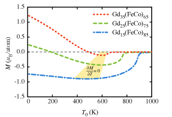
Figure 3: (Color online) Equilibrium magnetization of Gd_x(FeCo)_1-x alloys as a function of temperature for three Gd concentrations, $x_{\mathrm{Gd}}=0.15,0.25,$ and $0.35$. The yellow shaded area represents the temperature region where $\partial M_{\mathrm{FeCoGd}}/\partial T\approx 0$.

In contrast to ferromagnets, where the net equilibrium magnetization $M(T)=M_{s}(T=0\ \mathrm{K})m(T)$ always decreases with increasing temperature, in RE-TM ferrimagnetic alloys more possibilities exist. As an example to illustrate this, we consider the disordered alloy Gd₂₅(FeCo)₇₅ (with the parameters of Ref. OstlerPRB2011, ). Here, as shown in Fig 2(a), the net magnetization goes through a transition at a “magnetization derivative” compensation temperature $T_{\textrm{tr}}$ at $\partial M_{\mathrm{net}}/\partial T=0$, where $M_{\mathrm{net}}=M_{\mathrm{Fe}}x_{{\mathrm{Fe}}}m_{\mathrm{Fe}}-M_{\mathrm{Gd}}x_{{\mathrm{Gd}}}m_{\mathrm{Gd}}$. Because of the slow variation of the magnetization around $T_{\textrm{tr}}$ (see Fig. 2(a)), it is most appropriate to define the temperatures around $T_{\textrm{tr}}$ as a region in which a transition between two different demagnetization rates occur. We will show that this is the area in which a transition occurs between the two polarizations of the transient state. This is dependent on the alloy concentration as illustrated in Fig. 3, which shows the equilibrium magnetization of Gd_x(FeCo)_1-x alloys as a function of temperature for three Gd concentrations, $x_{\mathrm{Gd}}=0.15,0.25,$ and $0.35$. The yellow shaded area represents the temperature region where $\partial M_{\mathrm{FeCoGd}}/\partial T\approx 0$.

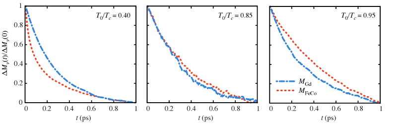
Figure 4: Dynamic relaxation after a step increase in temperature of the normalized magnetization of FeCo and Gd sublattices for three different temperatures as calculated from the atomistic approach. We use the normalization magnetization, $\Delta M_{\nu}(t)/\Delta M_{\nu}(0)$ rather than $M_{\nu}(t)$ to directly compare the relative magnetization relaxation dynamics of each sublattice. Note the change in relative relaxation rates from ’slow’ Gd at low temperatures to ’fast’ Gd approaching $T_{c}$.

Subsequently, and still for our exemplar alloy system Gd₂₅(FeCo)₇₅, we can define three well-defined temperature regions in terms of partial sublattice magnetization derivatives

$$\left|\frac{\partial M_{\mathrm{FeCo}}}{\partial T}\right|<\left|\frac{\partial M_{\mathrm{Gd}}}{\partial T}\right|\quad\mathrm{for}\quad T\lesssim\frac{3}{5}T_{c}\\$$ (6)

where the FeCo sublattice magnetization responds faster to temperature changes than the Gd sublattice. Around the point of inflection we have

$$\left|\frac{\partial M_{\mathrm{FeCo}}}{\partial T}\right|\approx\left|\frac{\partial M_{\mathrm{Gd}}}{\partial T}\right|\quad\mathrm{for}\quad\frac{3}{5}T_{c}\lesssim T\lesssim\frac{4}{5}T_{c}\\$$ (7)

and so both sublattices respond to temperature changes on a similar timescale. Finally for high temperatures close to $T_{c}$ we have

$$\left|\frac{\partial M_{\mathrm{FeCo}}}{\partial T}\right|>\left|\frac{\partial M_{\mathrm{Gd}}}{\partial T}\right|\quad\mathrm{for}\quad T_{c}\gtrsim T\gtrsim\frac{4}{5}T_{c}\\$$ (8)

indicating a temperature region where the FeCo sublattice magnetization responds slower than that of the Gd.

These criteria can be verified by comparing the quasi-equilibrium relaxation dynamics of each sublattice magnetization using the many-spin stochastic LLG equations (2), after a step like increase in temperature of $\Delta T=T_{0}/10$, as shown in Fig. 4. We present the results of our simulations in each regime, $T_{0}/T_{c}=0.4,0.85$ and $0.95$ ($T_{c}=800$ K). These results confirm the existence of the three distinct regions discussed previously. Most importantly, at temperatures very close to $T_{c}$ we do find that the Gd magnetization relaxes faster than that of the FeCo sublattice, contrary to the common perception that $\mu_{0}/T_{c}$ or $\mu_{0}/\lambda$ determine this timescale.KoopmansNatMat10 ; RaduNature2011 ; MentinkPRL2012

Therefore, our initial postulate that the relative speed of each magnetic lattice can be deduced from the value of $\partial M/\partial T$ is supported by the atomistic simulations. This is an important result relating the boundary between regimes of dynamic behavior to the relatively straightforward measurement of a static magnetic property. If this finding is experimentally confirmed, it will be very useful in the design of new materials showing novel ultrafast switching properties. However, this criterion alone does not provide a direct quantitative description of the relaxation behavior from the magnetic properties of the system. In the following we investigate the magnetization dynamics using an analytical approach based on the ferrimagnetic LLB equation. This provides an important basis for the interpretation of the detailed dynamic behavior calculated using the atomistic spin model.

II.5 Relaxation times derived from the Landau-Lifshitz-Bloch equation

Atomistic spin modeling has proved very adept at describing the non-equilibrium spin dynamics of GdFeCo in direct comparison with those observed in experiments.RaduNature2011 ; OstlerNatureComm2012 ; WienholdtPRL12 However, the many body nature of this approach makes the physical interpretation of results difficult. Moreover, a priori predictions are not possible from such an approach. In contrast, the macroscopic Landau-Lifshitz-Bloch (LLB) equationGaraninPRB1997 provides analytical expressions for the relaxation rates in terms of the magnetic properties of the system. The LLB equation describes the non-equilibrium average magnetization dynamics and is derived starting from the Heisenberg Hamiltonian (1) and the Fokker-Planck equation based on the atomistic Landau-Lifshitz equation thus providing a macroscopic description of the atomistic dynamics. GaraninPRB1997 Hence, we will use the LLB model to give clear evidence for the heuristic relation presented previously between the relaxation time and the proposed criterion in terms of $\partial M/\partial T$.

The ferrimagnetic LLB equationAtxitiaPRB2012LLBferrim is written for the reduced magnetization of each sublattice, $\langle\mathbf{S}_{\nu}\rangle=\mathbf{m}_{\nu}=\mathbf{M}_{\nu}/M_{s,\nu}$, where ${\nu}$ denotes TM or RE sublattice and $M_{s,\nu}$ is the saturation magnetization at $T=0$ K

$$\frac{\mathrm{d}\mathbf{m}_{\nu}}{\mathrm{d}t} = -|\gamma_{\nu}|\mathbf{m}_{\nu}\times\Big{[}\mathbf{H}_{\text{eff}}^{\nu}+\frac{\alpha^{\nu}_{\perp}}{m^{2}_{\nu}}\mathbf{m}_{\nu}\times\mathbf{H}_{\text{eff}}^{\nu}\Big{]}+|\gamma_{\nu}|\alpha^{\nu}_{\|}H_{\|}^{\nu}\mathbf{m}_{\nu}$$

The first two terms describe the motion of the transverse magnetization components, with a form form similar to the well-known Landau-Lifshitz-Gilbert equation, and which are driven by the effective field $\mathbf{H}_{\text{eff}}^{\nu}$ comprised of the usual anisotropy and applied fields. These two terms do not affect the pure longitudinal motion, the relaxation of which we are interested in. This Bloch-type (longitudinal) relaxation is described by the third term in Eq. (LABEL:eq:LLBferrimagFinalexpression1). Therefore we will neglect the transverse components in the following to reduce the number of parameters in Eq. (LABEL:eq:LLBferrimagFinalexpression1). Given the dominance of the Bloch-type relaxation this is a reasonable assumption that results in useful analytic expressions. Thus, the longitudinal Bloch-type relaxation is defined by

$$\frac{\mathrm{d}m_{\nu}}{\mathrm{d}t}=|\gamma_{\nu}|\alpha^{\nu}_{\|}H_{\|}^{\nu}m_{\nu}.$$ (10)

To further simplify the interpretation of the relaxation rates defining this equation and since we are interested in the relative rather the absolute relaxation times we can assume $\gamma_{{\text{\tiny{TM}}}}=\gamma_{{\text{\tiny{RE}}}}$ and $\lambda_{\|}^{{\text{\tiny{T}}}}=\lambda_{\|}^{{\text{\tiny{R}}}}$. The longitudinal field $H_{\|}^{\nu}$ which defines the different dynamics of each sublattice reads

$$H_{\|}^{\nu} = \left[\frac{1}{2\Lambda_{\nu\nu}}\left(\frac{m_{\nu}^{2}}{m_{e,\nu}^{2}}-1\right)-\frac{1}{2\Lambda_{\nu\kappa}}\left(\frac{m_{\kappa}^{2}}{m_{e,\kappa}^{2}}-1\right)\right].$$ (11)

The subscript $e$ denotes the equilibrium values. The field in Eq. (11) is comprised of the difference between the relaxation of sublattice $\nu$ to its own equilibrium value and to the equilibrium value of the $\kappa$ sublattice. The relaxation parameters are defined in Table 1. They are expressed in term of a physically measurable longitudinal susceptibilities. The latter can be also evaluated in the MFA approximation as

$$\chi^{\nu}_{\|}=\frac{\mu_{\kappa}}{|J_{0,\kappa\nu}|}\frac{-|J_{0,\nu\kappa}||J_{0,\kappa\nu}|\beta^{2}\mathcal{L}_{\kappa}^{{}^{\prime}}(.)\mathcal{L}_{\nu}^{{}^{\prime}}(.)+(\mu_{\nu}/\mu_{\kappa})|J_{0,\kappa\nu}|\beta\mathcal{L}_{\nu}^{{}^{\prime}}(.)(1-J_{0,\kappa}\beta\mathcal{L}_{\kappa}^{{}^{\prime}}(.))}{(1-J_{0,\kappa}\beta\mathcal{L}_{\kappa}^{{}^{\prime}}(.))(1-J_{0,\nu}\beta\mathcal{L}_{\nu}^{{}^{\prime}}(.))-|J_{0,\nu\kappa}||J_{0,\kappa\nu}|\beta^{2}\mathcal{L}_{\kappa}^{{}^{\prime}}(.)\mathcal{L}_{\nu}^{{}^{\prime}}(.)}$$ (12)

where the parameter definitions are given in table 1. We note that the relaxation parameters in Eq. (12) depend on the exchange and the atomic magnetic moments of both sublattices.

Parameter	Expression	Description
$\Lambda_{\nu\kappa}$	$|J_{0,\nu\kappa}|/\mu_{\nu}m_{e,\nu}/$	Relaxation parameter
$\Lambda_{\nu\nu}$	$\widetilde{\chi}^{\nu}_{\|}/\left(1-|J_{0,\nu\kappa}|\widetilde{\chi}^{\kappa}_{\|}/\mu_{\nu}\right)$	Relaxation parameter
$\alpha_{\|}^{\nu}$	$2\lambda_{\nu}/\beta\widetilde{J}_{0,\nu}$	Longitudinal damping
$\alpha_{\bot}^{\nu}$	$\lambda_{\nu}(1-1/\beta\widetilde{J}_{0,\nu})$	Perpendicular damping
$\widetilde{J}_{0,\nu}$	$J_{0,\nu}+|J_{0,\nu\kappa}|m_{e,\kappa}/m_{e,\nu}$	MFA exchange
$J_{0,\nu}$	$x_{\nu}zJ_{\nu\nu}$	Intra-lattice exchange
$J_{0,\nu\kappa}$	$x_{\kappa}zJ_{\nu\kappa}$	Inter-lattice exchange

Table 1: Explicit expressions of the parameters entering Eqs. (LABEL:eq:LLBferrimagFinalexpression1) and (11). $\widetilde{\chi}^{\nu}_{\|}=\left(\partial m_{\nu}/\partial H\right)_{H\rightarrow 0}$, and $m_{e,\nu}$ are calculated using the MFA AtxitiaPRB2012LLBferrim $\beta=1/k_{\mathrm{B}}T$. $x_{\nu}$ is the concentration of the specie $\nu$ and $z$ the number of nearest neighbours.

To calculate the relaxation rates of each sublattice, the system of coupled LLB equations (LABEL:eq:LLBferrimagFinalexpression1) is linearized by assuming small deviations from equilibrium, $m_{{\text{\tiny{TM(RE)}}}}=m_{e,{\text{\tiny{TM(RE)}}}}+\delta m_{{\text{\tiny{TM(RE)}}}}$ and $\delta\mathbf{m}=(\delta m_{\text{\tiny{TM}}},\delta m_{\text{\tiny{RE}}})$. This gives a characteristic matrix, $\mathcal{A}_{\|}$, which drives the dynamics of the linearized equation $\partial(\delta\mathbf{m})/\partial t=\mathcal{A}_{\|}\delta\mathbf{m}$. The matrix $\mathcal{A}_{\|}$ reads

$$\mathcal{A}_{\|}=\left(\begin{array}[]{ccc}-\gamma_{{\text{\tiny{TM}}}}\alpha_{\|}^{{\text{\tiny{TM}}}}/\Lambda_{{\text{\tiny{TT}}}}&\gamma_{{\text{\tiny{TM}}}}\alpha_{\|}^{{\text{\tiny{TM}}}}J_{0,{\text{\tiny{TR}}}}/\mu_{{\text{\tiny{T}}}}\\ \gamma_{{\text{\tiny{RE}}}}\alpha_{\|}^{{\text{\tiny{RE}}}}J_{0,{\text{\tiny{RT}}}}/\mu_{{\text{\tiny{R}}}}&-\gamma_{{\text{\tiny{RE}}}}\alpha_{\|}^{{\text{\tiny{RE}}}}/\Lambda_{{\text{\tiny{RR}}}}\end{array}\right)=\left(\begin{array}[]{ccc}\Gamma_{{\text{\tiny{TT}}}}&\Gamma_{{\text{\tiny{TR}}}}\\ \Gamma_{{\text{\tiny{RT}}}}&\Gamma_{{\text{\tiny{RR}}}}\end{array}\right)$$ (13)

It is important to note that the matrix elements in equation (13) are temperature dependent. The general solution of the characteristic equation, $|\mathcal{A}_{\|}-\Gamma^{\pm}\mathcal{I}|=0$, gives two different eigenvalues, $\Gamma^{\pm}=1/\tau_{\pm}$, corresponding to the eigenvectors $\mathbf{v}_{\pm}=(\Gamma_{{\text{\tiny{TR}}}},-(\Gamma_{{\text{\tiny{TT}}}}+\Gamma^{\pm}))$. In ferromagnets, relaxation can usually be described well by only one relaxation rate, at least in the linear regime. By contrast, in two sublattice ferrimagnets, a combination of the two characteristic relaxation rates $\Gamma^{\pm}$ describes the magnetization relaxation of each sublattice with a weighting determined by the eigenvectors. This means that one cannot describe the relaxation of a two-component system with as single exponential decay function except in some limits that we will consider next.

Figure 2 (b) shows the temperature dependence of the matrix elements Eq. (13), for a Gd₂₅(FeCo)₇₅ alloy. At temperatures far from $T_{c}$, $T\leq(3/4)T_{c}$, the relaxation rates fulfill the conditions $\Gamma_{{\text{\tiny{TT}}}}\gg\Gamma_{{\text{\tiny{RR}}}}>\Gamma_{{\text{\tiny{RT(TR)}}}}$. Therefore the motion of each sublattice is approximately defined by the corresponding diagonal element, i.e. $\partial\delta m_{{\text{\tiny{TM(RE)}}}}/\partial t=-\Gamma_{{\text{\tiny{TT(RR)}}}}\delta m_{{\text{\tiny{TM(RE)}}}}$, or equivalently, each eigenvector is associated with one sublattice. The relaxation rates ($\tau^{-1}$) are $-\gamma_{\nu}\alpha_{\|}^{\nu}/\Lambda_{\nu\nu}$, ($\nu=$RE, TM). It has been shown that $\gamma_{{\text{\tiny{RE}}}}\alpha_{\|}^{{\text{\tiny{RE}}}}\approx\gamma_{{\text{\tiny{TM}}}}\alpha_{\|}^{{\text{\tiny{TM}}}}$, AtxitiaPRB2012 thus the leading contribution to the temperature dependence of the demagnetization times comes from the parameters $\Lambda_{\nu\nu}$ which can be regarded as an effective longitudinal susceptibility in analogy with the pure ferromagnetic case. This parameter in turn depends on the actual longitudinal susceptibilities as

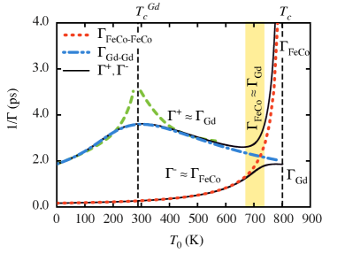
Figure 5: Characteristic relaxation times in GdFeCo alloy as a function of temperature. At relatively low temperatures $\Gamma^{+}\approx\Gamma_{\mathrm{Gd}}$ and $\Gamma^{-}\approx\Gamma_{\mathrm{FeCo}}$. The Gd relaxation time presents a maximum at $T_{c}^{\mathrm{Gd}}$ caused by the slowing down of the Gd fluctuations related to Gd-Gd interactions. The yellow shaded area corresponds to a mixed relaxation times and both sublattices relax similarly. Close to $T_{c}$, $\Gamma_{\mathrm{Gd}}\gg\Gamma_{\mathrm{FeCo}}$, and Gd sublattice magnetization relaxes faster.

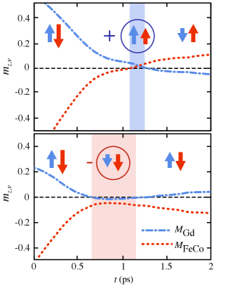
Figure 6: (Color online) (up) A positive TFLS means that the FeCo sublattice reverses first after the application of a laser heat pulse, (down) and a negative TFLS that the Gd sublattice reverses.

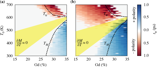
Figure 7: (Color online) (a) and (b) phase diagrams of the TFLS duration and polarity as a function of the initial temperature $T_{0}$ and Gd concentration for a heat step pulse of $600$ fs and $T_{\mathrm{max}}=1200$ K (a) and $T_{\mathrm{max}}=1500$ K (b) gained by computer atomistic simulations. A positive TFLS means that the FeCo sublattice reverse first, and a negative TFLS that Gd sublattice does. The dashed line in (a) and (b) corresponds to the transition temperature $T_{\mathrm{tr}}$ and $T_{\mathrm{M}}$. For low excitation heat pulses ($T_{\mathrm{max}}$=1200 K in (b)) these characteristic temperatures define well the regions where the TFLS can be encountered and its polarity.

$$\tau_{\|}^{\nu}=\frac{\Lambda_{\nu\nu}(T)}{\gamma_{\nu}\alpha^{\nu}_{\|}}=\frac{1}{\gamma_{\nu}\alpha^{\nu}_{\|}}\frac{\widetilde{\chi}^{\nu}_{\|}(T)}{1+\frac{J_{0,\nu\kappa}}{\mu_{\nu}}\widetilde{\chi}^{\kappa}_{\|}(T)}.$$ (14)

Equation (14) allows us to analyze the differences between both magnetic sublattices for $T_{0}\leq(3/4)T_{c}$. For RE concentrations $(x=0.2-0.3)$ where the TFLS has been experimentally observed, the mean field exchange interaction between TM and RE spins can be neglected, $J_{0,{\text{\tiny{TR}}}}=xzJ_{{\text{\tiny{TR}}}}$ is small given that $J_{0,{\text{\tiny{TT}}}}\gg J_{0,{\text{\tiny{TR}}}}$. This leads to the approximate form of Eq. (14) as $\gamma_{{\text{\tiny{TM}}}}\alpha^{{\text{\tiny{TM}}}}_{\|}\tau_{\|}^{{\text{\tiny{TM}}}}(T)=\widetilde{\chi}^{{\text{\tiny{TM}}}}_{\|}(T)\propto\mu_{{\text{\tiny{TM}}}}/J_{0,{\text{\tiny{TT}}}}$. This dependence reflects the fact that the TM relaxation is mainly determined by the exchange interaction between TM neighbors because each atomic TM moment is almost totally surrounded by other TM moments ($1-x=0.7-8$). The RE relaxation is determined by the antiferromagnetic exchange coupling with the TM neighbors $J_{0,{\text{\tiny{RR}}}}=xzJ_{{\text{\tiny{RR}}}}$ which is small due to the small probability that any RE moments interact with a RE nearest neighbor at low RE concentrations. At low temperatures and rare earth concentrations, one can consider the limiting case of a dilute paramagnetic rare earth species within a transition metal bulk. Using $(J_{0,{\text{\tiny{TR}}}}/\mu_{{\text{\tiny{RE}}}})\widetilde{\chi}_{\|}^{{\text{\tiny{TM}}}}\ll 1$, from Eq. (14) one obtains that that $\gamma_{{\text{\tiny{RE}}}}\alpha^{{\text{\tiny{RE}}}}_{\|}\tau_{\|}^{{\text{\tiny{RE}}}}=\widetilde{\chi}^{{\text{\tiny{RE}}}}_{\|}(T)$, which explains the local maximum in $\Gamma_{\mathrm{Gd}}$ at $T_{c}^{\mathrm{Gd}}=291$ K and which is related to the slowing down due to ferromagnetic Gd-Gd interactions [dashed lines in Fig. 5]. In this temperature region, the relevant magnetic parameter defining the RE magnetization relaxation is $\gamma_{{\text{\tiny{RE}}}}\alpha^{{\text{\tiny{RE}}}}_{\|}\tau_{\|}^{{\text{\tiny{RE}}}}=\mu_{{\text{\tiny{RE}}}}/|J_{0,{\text{\tiny{RT}}}}|$ and we obtain:

$$\frac{\tau^{{\text{\tiny{RE}}}}_{\|}}{\tau^{{\text{\tiny{TM}}}}_{\|}}\sim\frac{\mu_{{\text{\tiny{RE}}}}|J_{0,{\text{\tiny{TT}}}}|}{\mu_{{\text{\tiny{TM}}}}|J_{0,{\text{\tiny{RT}}}}|}\gg 1.$$ (15)

As temperature increases, the off diagonal terms in matrix equation $|\mathcal{A}_{\|}-\Gamma^{\pm}\mathcal{I}|=0$ start to play an increasing role. It is no longer possible to attribute one eigenvector to one sublattice but instead there are mixed contributions from both sublattices. This means that both the TM and RE sublattices relax with a similar mix of the two characteristic times, $\Gamma^{\pm}$ [grey zone in Fig. 5]. Both sublattices are magnetically equivalent in terms of relaxation rates around some temperature $T_{\text{tr}}$, where $\Gamma_{{\text{\tiny{TT}}}}\approx\Gamma_{{\text{\tiny{RR}}}}$ holds. This finding clearly shows that the simple ratio between atomic magnetic moments $\mu_{{\text{\tiny{TM}}}}/\mu_{{\text{\tiny{RE}}}}$ is no longer a sufficiently good estimate of the non-equivalence of the sublattice relaxation times.

Above $T_{\text{tr}}$ and approaching $T_{c}$, the TM relaxation time becomes longer than that of the RE. The TM is undergoing critical slowing down towards $T_{c}$ RushbrookeBook due to the divergence of $\widetilde{\chi}^{{\text{\tiny{TM}}}}_{\|}$ [see Fig. 5]. The RE relaxation time is only slightly temperature dependent even approaching $T_{c}$ as $\gamma_{{\text{\tiny{RE}}}}\alpha^{{\text{\tiny{RE}}}}_{\|}\tau_{\|}^{{\text{\tiny{RE}}}}=\mu_{{\text{\tiny{RE}}}}/|J_{0,{\text{\tiny{RT}}}}|\left(\widetilde{\chi}^{{\text{\tiny{TM}}}}_{\|}/\widetilde{\chi}_{\|}^{{\text{\tiny{RE}}}}\right)$, where the ratio between partial susceptibilities does not strongly depend on temperature. AtxitiaPRB2012LLBferrim

We conclude that $T_{\text{tr}}$ separates two non-equivalence regimes for the element specific magnetization dynamics. Though this result is strictly applicable only in the linear regime (small deviations from equilibrium), we show next that it can be extended for the laser heating induced TFLS and a similar transition can be observed.

III Control of the TFLS polarity

With our knowledge of these two non-equivalent regimes, we shall demonstrate that one may selectively excite a certain polarity depending on the composition of the alloy and the initial temperature. To do so, we use the atomistic spin model described by the Hamiltonian (1) and the set of atomistic LLG equations (2) to perform extensive computer simulations of pump-probe laser heating experiments in GdFeCo alloys for a range of Gd concentrations, initial temperatures, and laser fluence. The dynamical behavior of $T_{e}(t)$ after the application of a femtosecond laser pulse has been shown to be well reproduced by the two-temperature model (2TM).Chen2006 Within this model the electron and phonon systems are described as heat baths with associated temperatures $T_{e}(t)$ and $T_{ph}(t)$. The laser pulse heats the electron system which increases its temperature in the timescale of the order of hundreds of femtoseconds, to around 1000 to 2000 K, afterwards the electron system cools down by transferring energy to the phonon system in the picosecond time scale through the electron-phonon coupling. In our current calculations, this model is simplified by considering that the effect of the laser is to increase the electron temperature from the initial temperature $T_{0}$ to $T_{\textrm{max}}$ and then to reduce back to $T_{0}$ (a temperature step with $600$ fs duration in our model). We use this simple profile for the electron temperature so that we may disentangle the magnetization dynamics from the effect of different temperature profiles which are usually considered in ultrafast pump-probe experiments.

The results in Fig. 6 clearly show that the TFLS can be formed in either TM (+) or RE (-) polarities. This depends on the initial temperature and the Gd concentration. In Fig. 7(a),(b) we calculate the polarity and duration of the TFLS for two different pulse powers with $T_{\textrm{max}}=1200$ and $1500$ K, representing a low and high power input. The coloring, red or blue, represents the polarity of the state formed and the intensity of the color represents the duration. The result with a low power input ($T_{\mathrm{max}}=1200$ K) is that the transition temperature $T_{\mathrm{tr}}$ lies close to our theoretical prediction, $T_{\mathrm{tr}}$. This happens because the temperature difference between $T_{0}$ and $T_{\mathrm{max}}$ at high temperatures when $T_{0}\approx T_{c}$ is not very large, and the pulse duration is short so the dynamics are still within the linear regime. The positive polarity, the one already observed experimentally (blue area), follows the $T_{M}$ line, supporting the ferrimagnetic exchange mode excitation described in detail in Sec. II.2.

For a higher power input ($T_{\mathrm{max}}=1500$ K), Fig. 7(b), the TFLS is formed beyond the boundary of our predicted transition temperature, because the linear approximation is no longer valid. Nonetheless, the qualitative shape of these regions is still captured by our theoretical curves. This confirms that the insights gained from our theoretical estimations based on the LLB model still are useful in such highly non-equilibrium situations.

In both high and low power examples, the region of relaxation time equivalence (marked in yellow) prohibits the formation of a TFLS as we had expected. This result gives a clear link between the equilibrium temperature measurements that are likely to be easily measured in experiments and the non-equilibrium ultrafast laser induced control of the transient ferromagnetic-like state in ferrimagnets.

The experimental verification of our findings is a real challenge since initial high temperature measurements using element specific femtosecond resolution XMCD would not be straightforward due to the small magnetic signals expected. However, recent experiments in CoTb alloys have shown that Tb magnetization demagnetizes faster as the ratio $T_{0}/T_{c}$ increases. LopezfloresArxiv2013 To demonstrate this they used different Tb concentrations rather than changing the initial temperature. This result agrees with our findings. In addition, recent experiments GravesNatureMaterials2013 measured the spatial distribution of FeCo and Gd atoms in a heterogeneous GdFeCo alloy, showing significant clustering of the RE and TM species into regions with large correlation lengths. Using time resolved XMCD that probed nanoscale spin dynamics they found that, for some Gd-rich regions (equivalent to our high Gd concentration alloys), the transient ferromagnetic like state has Gd polarity. Graves et al. GravesNatureMaterials2013 associated this behavior with a non-local magnetization transfer between Gd-rich and FeCo-rich regions by superdiffusive spin transport. This observation also provides at least indirect support for the formation of the RE- driven TFLS polarity predicted here. Moreover, the laser heating in their work completely demagnetizes the sample, i.e. a high laser fluence scenario and we know from Fig. 7 that with a higher fluence the negative polarity state becomes more prevalent. A direct comparison between Fig. 7 and these experiments is not possible due to the macroscopic clustering found by Graves et al. GravesNatureMaterials2013 which will cause a distribution of effective Curie temperatures in the sample. Also, the sensitively of the results to the Curie temperatures and compensation temperatures mean that a more detailed knowledge of the magnetic properties of their sample would be needed for a direct comparison. Our results however, show that non-local angular momentum transfer is not necessary to interpret their experimental findings if one applies our theory.

IV Conclusions

In summary, we have shown that the femtosecond laser induced transient ferromagnetic-like state (TFLS) polarity in rare earth-transition metal (RE-TM) ferrimagnets can be controlled by tuning the initial temperature and Gd impurity concentration. We have demonstrated that a non-equivalent heating efficiency of the two sublattices is a key criterion for the formation of the TFLS. To show this, we have studied in detail the RE-TM ferrimagnetic GdFeCo alloy and shown that due to the different nature of the spin fluctuations the magnetic response of each sublattice depends distinctly on the temperature. Microscopically, the magnetization dynamics of the TM sublattice is dominated by ferromagnetic fluctuations that slow down its dynamics approaching $T_{c}$. The dynamics of the rare-earth impurities are dominated by antiferromagnetic fluctuations that make its dynamics almost temperature independent. Therefore, our results predict that, at high temperatures, the conventionally slow relaxing rare earth magnetic impurities may become faster than the transition metal magnetization. Our results highlight the requirement for the two sublattices to have different relaxation times in order to form a TFLS which can lead to switching in the positive polarity. In the region of equivalence in the relaxation rate of the two sublattices, no TFLS can be formed and therefore switching is also prohibited. These results could have important implications for the design of future all-optical THz devices since we have also provided a simple picture of this non-equivalence in terms of measurable quantities, $M(T)$ and $\partial M/\partial T$, with the further advantage that it can be generalized to other multi-sublattice alloys.

V Acknowledgement

This work was supported by the Spanish Ministry of Science and Innovation under the grant FIS2010-20979-C02-02 and by the European Community’s Seventh Framework Programme (FP7/2007-2013) under grant agreement No. 281043, FEMTOSPIN. U.A. gratefully acknowledges support from Basque Country Government under ”Programa Posdoctoral de perfeccionamiento de doctores del DEUI del Gobierno Vasco”.

References

- (1) I. Radu, K. Vahaplar, C. Stamm, T. Kachel, N. Pontius, H. A. Dürr, T. A. , J. Barker, R. F. L. Evans, R. W. Chantrell, A. Tsukamoto, A. Itoh, A. Kirilyuk, Th. Rasing and A. V. Kimel, Nature, 472, 205 (2011).
- (2) T. A. Ostler, J. Barker, R. F. L. Evans, R. W. Chantrell, U. Atxitia, O. Chubykalo-Fesenko, S. El Moussaoui, L. Le Guyader, E. Mengotti, L. J. Heyderman, F. Nolting, A. Tsukamoto, A. Itoh, D. Afanasiev, B. A. Ivanov, A. M. Kalashnikova, K. Vahaplar, J. Mentink, A. Kirilyuk, Th. Rasing, and A. V. Kimel, Nature Commun. 3, 666 (2012).
- (3) L. Le Guyader, S. El Moussaoui, M. Buzzi, R. V. Chopdekar, L. J. Heyderman, A. Tsukamoto, A. Itoh, A. Kirilyuk, Th. Rasing, A. V. Kimel, and F. Nolting, Appl. Phys. Lett. 101 022410 (2012)
- (4) A. Kirilyuk, A. V. Kimel, and Th. Rasing, Reports on Progress in Physics, 76, 026501 (2013)
- (5) J. Stöhr, and H. C. Siegmann, Magnetism: from Fundamentals to Nanoscale Dynamics (Springer, Berlin, 2006).
- (6) A. R. Khorsand, M. Savoini, A. Kirilyuk, A. V. Kimel, A. Tsukamoto, A. Itoh, and Th. Rasing, Phys. Rev. Lett., 110, 107205 (2013)
- (7) J. H. Mentink, J. Hellsvik, D. V. Afanasiev, B. A. Ivanov, A. Kirilyuk, A. V. Kimel, A. V. O. Eriksson, M. I. Katsnelson, and Th. Rasing, Phys. Rev. Lett. 108 057202 (2012).
- (8) N. Kazantseva, U. Nowak, R. W. Chantrell, J. Hohlfeld and A. Rebei, Europhys. Lett. 81 27004 (2008)
- (9) A. J. Schellekens, and B. Koopmans, Phys. Rev. B 87 020407 (2013).
- (10) U. Atxitia, T. Ostler, J. Barker, R. F. L. Evans, R. W. Chantrell and O. Chubykalo-Fesenko, Phys. Rev. B 87 224417 (2013)
- (11) J. Barker, U. Atxitia, T. A. Ostler, H. Ovorka, O. Chubykalo-Fesenko, and R. W. Chantrell, Scientific Reports, 3 3262 (2013)
- (12) R. F. L.Evans, T. A. Ostler, R. W. Chantrell, I. Radu, and Th. Rasing arxiv.1310.5170v1 (2013)
- (13) U. Atxitia and O. Chubykalo-Fesenko, Phys. Rev. B 84, 144414 (2011)
- (14) B. Koopmans, G. Malinowski, F. Dalla Longa, D. Steiauf, M. Faehnle, T. Roth, M. Cinchetti, and M. Aeschlimann Nature Materials 9 259 (2010)
- (15) S. Alebrand, M. Gottwald, M. Hen, D. Steil, M. Chinchetti, D. Lacour, E. E. Fullerton, M. Aeschlimann, and S. Mangin, Appl. Phys. Lett. , 162408 (2012)
- (16) T. A. Ostler, J. Barker, R. F. L. Evans, R. W. Chantrell, U. Atxitia, O. Chubykalo-Fesenko, S. El Moussaoui, L. Le Guyader, E. Mengotti, L. J. Heyderman, F. Nolting, A. Tsukamoto, A. Itoh, D. Afanasiev, B. A. Ivanov, A. M. Kalashnikova, K. Vahaplar, J. Mentink, A. Kirilyuk, Th. Rasing and A. V. Kimel, Phys. Rev. B. 84, 024407 (2011).
- (17) T. Roth, A. J. Schellekens, S. Alebrand, O. Schmitt, D. Steil, B. Koopmans, M. Cinchetti, M. Aeschlimann, Phys. Rev. X, 2, 021006, (2012).
- (18) U. Atxitia, O. Chubykalo-Fesenko, J. Walowski, A. Mann and M. Münzenberg, Phys. Rev. B, 81, 174401 (2010).
- (19) J. Mendil, P. Nieves, O. Chubykalo-Fesenko, J. Walowski, M. Munzenberg, T. Santos, and S. Pisana, arXiv:1306.3112v1
- (20) V. Lopez-Flores, N. Bergeard, V. Halte, C Stamm, N. Pontius, M. Hehn, E. Otero, E. Beaurepaire, C. Boeglin, Phys. Rev. B, 87, 214412 (2013)
- (21) R. Medapalli, I. Razdolski, M. Savoini, A. R. Khorsand, A. M. Kalashnikova, A.Tsukamoto, A. Itoh, A. Kirilyuk, A. V. Kimel, Th. Rasing, Eur. Phys. J. B. 86, 183 (2013)
- (22) J. G. S. Rushbrooke and G. A. Baker, Phase Transitions and Critical Phenomena (Academic, New York, 1974), Vol. 3.
- (23) U. Atxitia, P. Nieves, and O. Chubykalo-Fesenko, Phys. Rev. B , 104414 (2012).
- (24) R. M. Bozorth, Ferromagnetism (IEEE, New York, 2003).
- (25) J. Jensen and A. R. Mackintosh, Rare Earth Magnetism: Structures and Excitations (Clarendon, Oxford, 1991).
- (26) U. Atxitia, O. Chubykalo-Fesenko, R. W. Chantrell, U. Nowak, and A. Rebei Phys. Rev. Lett. 102 057203 (2009)
- (27) N. Kazantseva , et al. Phys. Rev. B 184428 (2008)
- (28) S. Wienholdt, D. Hinzke, K. Carva, P.M. Oppeneer, and U. Nowak Phys. Rev. B, 88, 020406 (2013)
- (29) M. Sultan, U. Atxitia, A. Melnikov, O. Chubykalo-Fesenko, U. Bovensiepen, Phys. Rev. B , 184407 (2012)
- (30) M. O. A. Ellis, T. A. Ostler, and R. W. Chantrell, Phys. Rev. B 86, 174418 (2012)
- (31) C. D. Stanciu, F. Hansteen, A. V. Kimel, A. Kirilyuk, A. Tsukamoto, A. Itoh, Th. Rasing, Phys. Rev. Lett.
- (32) A. Mekonnen, M. Cormier, A. V. Kimel, A. Kirilyuk, A. Hrabec, L. Ranno, and T. Rasing, Phys. Rev. Lett. 107, 117202 (2011).
- (33) F. Schlickeiser, U. Atxitia, S. Wienholdt, D. Hinzke, O. Chubykalo-Fesenko, and U. Nowak, Phys. Rev. B 86 214416 (2012)
- (34) A. Hassdenteufel, B. Hebler, C. Schubert, A. Liebig, M. Teich, M. Helm, M. Aeschlimann, M. Albrecht, and R. Bratschitsch, Adv. Mat. 25 3122 (2013)
- (35) S. Wienholdt, D. Hinzke, U. Nowak, Phys. Rev. Lett. 108, 247207 (2012).
- (36) S. Alebrand, A. Hassdenteufel, D. Steil, M. Cinchetti, M. Aeschlimann Phys. Rev. B 85, 092401 (2012)
- (37) A. Mann, J. Walowski, M. Munzenberg, S. Maat, M. J. Carey, J. R. Childress, C. Mewes, D. Ebke, V. Drewello, G. Reiss, A. Thomas, Phys. Rev. X 2, 041008 (2012).
- (38) M. Battiato, K. Carva, and P. M. Oppeneer, Phys. Rev. Lett. 105, 027203 (2010)
- (39) B. Y. Mueller, A. Baral, S. Vollmar, M. Cinchetti, M. Aeschlimann, H. C. Schneider, and B. Rethfeld, Phys. Rev. Lett. 111 167204 (2013)
- (40) M. Wietstruk, A. Melnikov, C. Stamm, T. Kachel, N. Pontius, M. Sultan, C. Gahl, M. Weinelt, H. A. Durr, and U. Bovensiepen, Phys. Rev. Lett. 106, 127401 (2011).
- (41) A. J. Schellekens, and B. Koopmans. Phys. Rev. Lett. 110, 217204 (2013).
- (42) A. Manchon, Q. Li, L. Xu, and S.Zhang, 85 064408, Phys. Rev. B (2012)
- (43) D. A. Garanin, Physica A 172, 470 (1991)
- (44) P. Nieves, D. Serantes, U. Atxitia, and O. Chubykalo-Fesenko, unpublished.
- (45) B. Koopmans, J. J. Ruigrok, F. D. Longa, and W. J. de Jonge, Phys. Rev. Lett. 95 267207(2005)
- (46) D. A. Garanin, Phys. Rev. B , 3050 (1997)
- (47) J. K. Chen, D. Y. Tzou, and J. E. Beraun, Int. J. Heat Mass Transfer 49, 307-316 (2006).
- (48) C. E. Graves, A. H. Reid, T. Wang, B. Wu, S. de Jong, K. Vahaplar, I. Radu, D. P. Bernstein, M. Messerschmidt, L. Müller, R. Coffee, M. Bionta, S. W. Epp, R. Hartmann, N. Kimmel, G. Hauser, A. Hartmann, P. Holl, H. Gorke, J. H. Mentink, A. Tsukamoto, A. Fognini, J. J. Turner, W. F. Schlotter, D. Rolles, H. Soltau, L. Struder, Y. Acremann, A. V. Kimel, A. Kirilyuk, Th. Rasing, J. Stohr, A. O. Scherz and H. A. Durr, Nat. Materials, 12 293 (2013)