Geometrical Probability Distribution Functions for Cable-in-Conduit Conductors with Simply and Multiply Connected Cross-Sections

Abstract

A geometrical method is presented for the calculation of the strand distribution functions for cable-in-conduit superconductors with simple and multiply connected cross-sections. The method is illustrated on different cable designs with simply and multiply connected structures. We start with the simple case of a round cable (a simply connected structure) and continue with some multiply connected structures: a cable with a central channel then one with a central channel and wrapped petals and finally a cable with segregated copper and central channel. Analytical relations are given which can be used in numerical simulations to calculate average values of certain cable properties like the average electric field.

I Introduction

A cable-in-conduit conductor (CICC) is usual made of a bunch of strands encapsulated in a metal conduit. The bunch consists of a large number of strands, around 1000, twisted together in many different stages, starting from a simple basis unit. Usually this is a triplet, a twist of three strands, but cables where the basic unit is a more complicated build such as a copper core surrounded by a number of superconducting strand twisted around it or even a relatively large braid are known. Not all strands in the cable are or should be by necessity superconducting. Segregated copper strands ca replace some of the superconducting ones either at the level of the basic unit or at higher stages. For example, instead of a full superconducting triplet one can have a triplet with the structure 2S+1Cu consisting of two superconducting and one copper wires. Alternatively, copper segregation can be produced by inserting copper wires or copper subcables in the cabling process at certain upper stages. The cross-section of the cable can be therefore very rich in structure showing either a dispersed segregation of copper wires if copper was introduced at the basic stage or islands of copper if copper is introduced at later stages. A typical cable in conduit conductor is shown in Fig.1

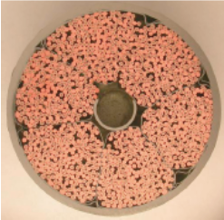
Figure 1: Color online. Typical Cable in Conduit Conductor with central channel and inter-petal void spaces.

Another source of inhomogeneity in the cable cross-section is related to the void spaces. Some cables are provided with a central channel added in order to improve the helium circulation and to reduce the pressure drop. In other cables the last stage (called “petal” for obvious reasons) is wrapped with a steel tape creating additional inter-petal spiral channels. In this respect we speak from cables which have a simply connected or a multiply connected structure.

Due to the self-field effect, the magnetic field distribution in the cable cross-section is not uniform. Through the dependence of critical current on field, the cable will show a non-uniform distribution of electric field in the cross-section if the volt-ampere characteristic of the strands is of power-law type. The measured electrical field(using voltage taps on the cable jacket) is a kind of average over an ensemble of strands. The calculation of the average electric field in a cable is based on the ergodic hypothesis ref1 which states that all strands trajectories are equivalent and the length average of one strand can be replaced by an ensemble average. This is similar to the principle from the statistical mechanics where the time average of a physical quantity can be replaced by an ensemble average. It was demonstrated in ref2 that for short length the ergodic hypothesis is not true and that in this case a statistical interpretation of the experimental results based on the central limit theorem should be made. For long cables sections however, with length of hundreds of the last stage twist pitch it seems, based on numerical simulation of strand trajectories, that the ergodic hypothesis holds ref2 . In this case the ensemble average can be calculated using a geometric probability distribution function as applied for the first time by Ekin ref3 for filaments in a strand and extended later in ref4 for simple connected full-size CICC. However, no mathematical proof exists for the time being that the twisted cables are ergodic for any number of stages and any combination of twist pitches.

According to Ekin’s proposalref3 , the average electric field (or any other observable) is calculated using the formula

$$\left\langle E\right\rangle\overset{\wedge}{=}\int{E\left(r\right)w\left(r\right)dr=\int{E\frac{dA_{E}}{A}}}$$ (1)

where $E\left(r\right)$ is the local electric field and $w\left(r\right)dr$ the probability density that a strand at position $r$ senses an electrical field $E(r)$

$$w\left(r\right)dr\overset{\wedge}{=}\frac{dN_{E}}{N}$$ (2)

with $dN_{E}$ the number of strands sensing the same electric field $E$ and $N$ is the total number of strands.

The last equality in Eq.(1) is based on the important assumption that the strands are distributed in the cable cross section such that a density (number of strands per unit area) can be defined. We assume therefore that we always can write

$$\begin{array}[]{c}dN_{E}=\rho dA_{E}\\ \\ N=\rho A\\ \end{array}$$ (3)

In the above equation, $\rho$ is the density of strands in the cable cross-section, $A$ is the total cable cross-sectional area and $dA_{E}$ represents a geometrical area element with the property that inside this area the electric field is constant. In other words it is the set of cable cross-section points having the same electrical field $E$

$$dA_{E}\overset{\wedge}{=}\left\{{r\in A\left|{E\left(r\right)=E}\right.}\right\}$$ (4)

In most of the cases of interest the density $\rho$ is constant and we we limit ourselves here to this case. Generalization to non uniform distribution of strands is straightforward and will be developed in the next sections. At this point it is important to make the difference between uniform density of strands and random strand position. A uniform density of strands in the cable cross section can be obtained also with strands twisted in concentric layers much similar to the superconducting filaments in the strand itself.Unfortunately this arrangement is not ergodic. By contrast, in multiple twisted cables the strands are much more randomly distributed as a consequence of the erratic overlapping of multiple twist stages with different (incommensurate) twist pitches. Therefore, it is generally believed that such cables satisfy the ergodicity condition. Therefore for the definition of the geometric probabilities we request first the randomness and then the uniform density. The randomness and ergodicity are the necessary conditions to calculate averages the way defined in Eq.(1).

The form of the elemental area can change from case to case. For the self-field problems it is a linear stripe perpendicular to the magnetic field gradient. For a round cable with transport current and no external field, the elemental area is a circular ring. The form of $dA_{E}$ should be therefore defined for each problem at hand but because in this paper we will discuss only the self-field effect the elemental area will be always a stripe as shown in Fig.2b.

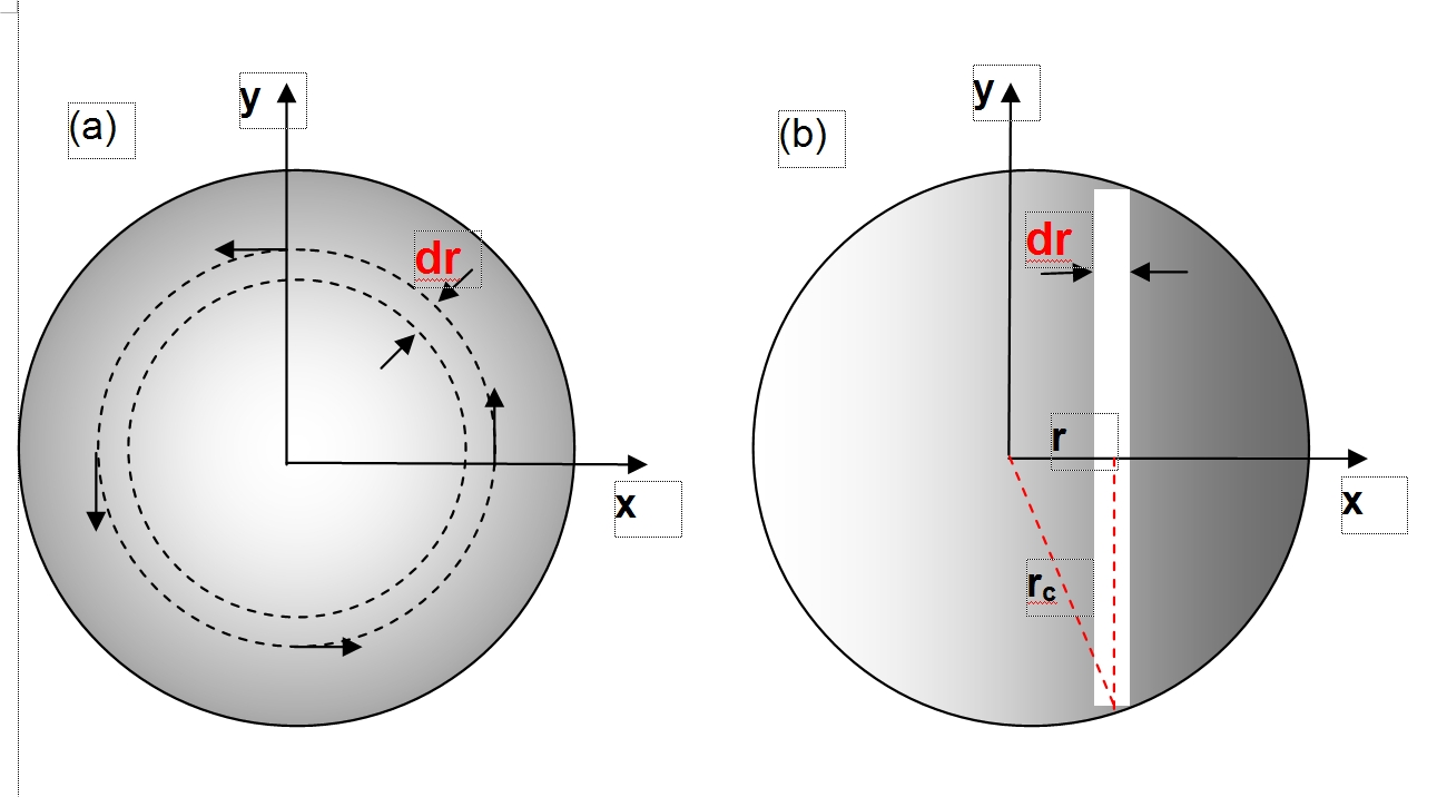
Figure 2: Color on line. Typical elemental areas for geometrical probability. a) no external field, self field has a radial distribution, b) superposition of an external uniform field (along Oy-axis) with the self-field of the cable results in a linear field distribution (field gradient) along the Ox-axis. Dark gray corresponds to higher magnetic field.

II Illustrative calculation for a simply connected cable contour

The simplest case of a simply connected cable is a circular cable without internal voids. As discussed above, the superposition of the uniform external field with the azimuthal field of the cable results in a linear variation of the magnetic over the cable cross-section. In this case the elemental area is a stripe (Fig.2b), parallel to the external field direction with area given by

$$dA_{E}=dA\left(r\right)=2\sqrt{r_{c}^{2}-r^{2}}dr$$ (5)

where $r_{c}$ is the cable radius and $r$ is the coordinate along the field gradient (Ox-axis in our case). The total cable cross-section area is

$$A=\pi r_{c}^{2}$$ (6)

and using Eqs.(2) and (3) we get the following expression for the probability distribution function

$$w_{0}\left(r\right)=\frac{2\sqrt{r_{c}^{2}-r^{2}}}{\pi r_{c}^{2}}$$ (7)

This is a strongly nonlinear function with a large slope close to $r=-r_{c}$ and $r=r_{c}$ and is represented graphically in Fig.3. Further, it can be checked by direct integration that $w_{0}\left(r\right)$, Eq.(7) satisfies the conditions of a probability distribution function i.e. we have first,

$$\int\limits_{-r_{c}}^{r_{c}}{w_{0}\left(r\right)dr=1}$$ (8)

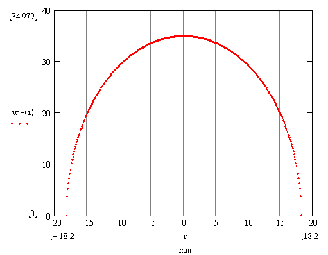
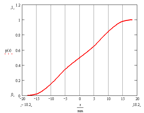
Figure 3: Color online. The probability distribution function $w_{0}(r)$(left panel) and the probability $p_{0}(r)$ (right panel), for a cable with a simple connected contour.

and second, the probability that a given strand is placed somewhere between $-r_{c}$ and $r$ is smaller than 1 for any $r\in[-r_{c},r_{c}]$

$$p_{0}\left(r\right)=\int\limits_{-r_{c}}^{r}{w_{0}\left(r\right)dr\leqslant 1}$$ (9)

The infinitesimal probability $dp_{0}$ is by definition

$$dp_{0}\left(r\right)\overset{\wedge}{=}w_{0}\left(r\right)dr=\frac{2\sqrt{r_{c}^{2}-r^{2}}}{\pi r_{c}^{2}}dr$$ (10)

Similarly, for a rectangular conductor of width $a$ and height $b$ as in Fig.4 we obtain

$$\begin{array}[]{l}w_{a}\left(x\right)dx=\dfrac{bdx}{ab}=\dfrac{1}{a}dx\mbox{ \quad\quad for }\nabla B\left\|a\right.\\ \\ w_{b}\left(x\right)dx=\dfrac{adx}{ab}=\dfrac{1}{b}dy\mbox{ \quad\quad for }\nabla B\left\|b\right.\\ \end{array}$$ (11)

In this case the elemental area is either $dA_{E}=b~{}dx$ or $dA_{E}=a~{}dx$ and the total area is $A=ab$. The probability distributions are both uniform but can differ substantially because $a<b$.

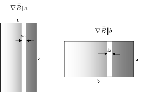
Figure 4: Geometrical parameters for rectangular conductor of width $a$ and height $b$. Left panel $\nabla B||a$, right panel $\nabla B||b$.

III General problem, multiple-connected cable contours

Multiple connected cables have holes or regions in the cross-sectional area occupied by another material and not by the superconducting strands. The holes could be for example the central channel or the inter-petal spaces for the conductors with wrapped last stage. Non homogeneous regions could be the copper islands in case of segregated copper cables. The holes and the inhomogeneous regions can be fixed ( they do not change the position in the cable cross-section as one moves along the cable axis) or itinerant ( they have variable position in the cable cross-section as one moves along the cable axis). The central channel is a good example of a fixed hole while the inter-petal spaces are itinerant holes. They rotate as part of the last stage with the same twist pitch as the cable’s last stage. As we will see later the area contribution of fixed holes and itinerant holes to the probability distribution function is quite different. The same holds for copper islands, although fixed copper islands are not found in the modern cable design.

In order to illustrate the calculation method for multiple connected cables let as refer to the geometry presented in Fig.5. The cable cross-section consists of two regions $A_{1}$ and $A_{2}$ with the property: $A=A_{1}\cup A_{2};\mbox{ }A_{1}\cap A_{2}=\emptyset$, where $\emptyset$ is the empty set. Transversally, there is a magnetic field gradient created by the superposition of the background field with the self field of the cable as shown in Fig.2.

For $|r|<r_{h}$ the infinitesimal probability is by definition

$$w_{r<r_{h}}\left(r\right)dr=\frac{dN_{1}+dN_{2}}{N}$$ (12)

with $dN_{i},\quad i=1,2$ the number of strands in the infinitesimal area $dA_{i}$. Assuming a uniform strand distribution in the two regions with densities $\rho_{1}$ and $\rho_{2}$ we have

$$\begin{array}[]{l}dN_{1}=\rho_{1}dA_{1};\mbox{ }dN_{2}=\rho_{2}dA_{2};\\ \\ N=\rho_{1}A_{1}+\rho_{2}A_{2};\mbox{ }A=A_{1}+A_{2}\end{array}$$ (13)

Substituting this back in Eq.12 we obtain

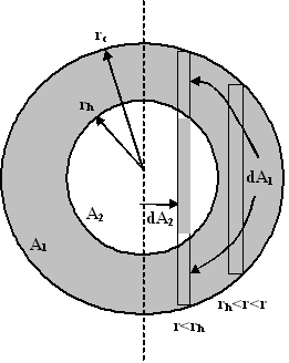
Figure 5: Geometry for a multiple connected cable

$$\begin{array}[]{c}w_{r<r_{h}}\left(r\right)dr=\dfrac{\rho_{1}dA_{1}+\rho_{2}dA_{2}}{\rho_{1}A_{1}+\rho_{2}A_{2}}=\\ \\ =\dfrac{\rho_{1}}{\rho_{1}A_{1}+\rho_{2}A_{2}}dA_{1}+\dfrac{\rho_{2}}{\rho_{1}A_{1}+\rho_{2}A_{2}}dA_{2}=\\ \\ =\dfrac{A}{A_{1}+\lambda A_{2}}\dfrac{dA_{1}}{A}+\dfrac{\lambda A}{A_{1}+\lambda A_{2}}\dfrac{dA_{2}}{A}\end{array}$$ (14)

with $\lambda={\rho_{2}}/{\rho_{1}}$.

For $r_{h}<|r|<r_{c}$ we have similarly

$$w_{r>r_{h}}(r)dr=\dfrac{dN_{1}}{N}=\dfrac{\rho_{1}dA_{1}}{\rho_{1}A_{1}+\rho_{2}A_{2}}=\dfrac{dA_{1}}{A_{1}+\lambda A_{2}}$$ (15)

An important special case is when $\rho_{2}=0$ i.e. when there is a central hole of area $A_{2}=\pi r_{h}^{2}$ in the cable cross section. In this case Eq.14 becomes

$$\begin{array}[]{c}w_{r<r_{h}}\left(r\right)dr=\dfrac{dA_{1}}{A_{1}}=\dfrac{dA_{1}}{A-A_{2}}=\dfrac{dA-dA_{2}}{A-A_{2}}=\\ \\ =\dfrac{2\left[{\sqrt{r_{c}^{2}-r^{2}}-\sqrt{r_{h}^{2}-r^{2}}}\right]}{\pi\left({r_{c}^{2}-r_{h}^{2}}\right)}dr\end{array}$$ (16)

and Eq.15

$$w_{r>r_{h}}=\dfrac{2\sqrt{r_{c}^{2}-r^{2}}}{\pi(r_{c}^{2}-r_{h}^{2})}$$ (17)

which gives finally the probability distribution function for a cable with a central channel of radius $r_{h}$

$$w_{h}\left(r\right)=\left\{{{\begin{array}[]{ll}{\dfrac{2\left[{\sqrt{r_{c}^{2}-r^{2}}-\sqrt{r_{h}^{2}-r^{2}}}\right]}{\pi\left({r_{c}^{2}-r_{h}^{2}}\right)}\mbox{\quad\quad for }\left|r\right|<r_{h}\hfill}\\ \\ {\dfrac{2\sqrt{r_{c}^{2}-r^{2}}}{\pi\left({r_{c}^{2}-r_{h}^{2}}\right)}\mbox{\quad\quad for }\left|r\right|>r_{h}\hfill}\\ \end{array}}}\right.$$ (18)

The probability density $w_{h}(r)$ and the probability function $p_{h}(r)$ calculated with Eq.18 are presented in Fig.6

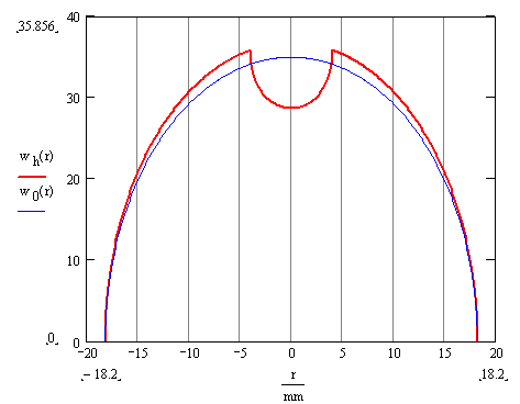
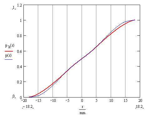
Figure 6: Color on line. The probability distribution function $w_{h}(r)$(left) and the probability $p_{h}(r)$ (right) for a cable with fixed hole in the central part of the cross-section. The blue line is the reference line for a compact cable, the probability density $w_{0}(r)$ and the probability $p_{0}(r)$.

The example presented above shows the calculation of the probability distribution function for a cable with a fixed hole in the middle of the cross-section, a typical example of a cable with a central channel. We are going to show now how to calculate the probability distribution function for a cable with four regions, two of which being itinerant. To be more precise, the object here is a cable in conduit conductor with wrapped last stage petals and a central channel. As shown in Fig.7 the first region is a strand region. Regions 2 and 3 are itinerant regions since they rotate through the cross-section, on advancing along the cable axis, with a period given by the the last twist pitch of the cable. These regions are created by the upper and lower inter-petal holes. The contribution of these two regions to the effective density is lower than that for the region one and we call them therefore diluted (or depleted) regions. Finally, there is a fourth region which is the central hole. This is fixed and has zero density contribution. The following equations are obtained by generalizing (extending) Eqs.13 and 14:

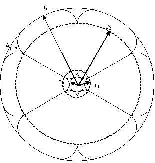
Figure 7: Example of a CICC with 6 wrapped petals in the last stage and a central hole. Observe the upper and lower inter-petal voids. They rotate along the conductor length and are therefore called itinerant holes (voids)as opposed to the central hole which is fixed. In this example $r_{c}$ =18.2 mm, $r_{2}$=15 mm, $r_{1}$ =6 mm and $r_{h}$ =4 mm.

$$\begin{array}[]{c}w\left(r\right)dr=\dfrac{\rho_{1}dA_{1}+\rho_{2}dA_{2}+\rho_{3}dA_{3}+\rho_{4}dA_{4}}{\rho_{1}A_{1}+\rho_{2}A_{2}+\rho_{3}A_{3}+\rho_{4}A_{4}}=\\ \\ A=A_{1}+A_{2}+A_{3}+A_{4}\\ \end{array}$$ (19)

the first expressing the definition of the probability density function and the second the total cross sectional area. The calculation proceeds in steps considering different ranges for the coordinate along the field gradient, $r$in the four regions. The four regions are

$$\begin{array}[]{l}\mbox{Region 1: }r_{2}<\left|r\right|\\ \\ \mbox{Region 2: }r_{1}<\left|r\right|<r_{2}\\ \\ \mbox{Region 3: }r_{h}<\left|r\right|<r_{1}\\ \\ \mbox{Region 4: }\left|r\right|<r_{h}\end{array}$$ (20)

In the first region we have

$$\begin{array}[]{c}\left[{w\left(r\right)dr}\right]_{1}=\dfrac{\rho_{2}dA_{2}}{\rho_{1}A_{1}+\rho_{2}A_{2}+\rho_{3}A_{4}}=\\ \\ =\dfrac{\lambda_{2}dA_{2}}{A_{1}+\lambda_{2}A_{2}+\lambda_{3}A_{3}}\end{array}$$ (21)

where we have defined

$$\lambda_{2}=\frac{\rho_{2}}{\rho_{1}};\mbox{ }\lambda_{3}=\frac{\rho_{3}}{\rho_{1}};\mbox{ }\lambda_{4}=\frac{\rho_{4}}{\rho_{1}}=0$$ (22)

where the last relation is for the central hole where no strand are present. Further we use the following relations:

$$\begin{array}[]{c}dA_{2}=2\left(\sqrt{r_{c}^{2}-r^{2}}\right)dr\\ \\ A_{1}=\pi\left({r_{2}^{2}-r_{1}^{2}}\right)\\ \\ A_{2}=\pi\left({r_{c}^{2}-r_{2}^{2}}\right)\\ \\ A_{3}=\pi\left({r_{1}^{2}-r_{h}^{2}}\right)\\ \\ A_{4}=\pi r_{h}^{2}\\ \\ \end{array}$$ (23)

The dilution factors for the two itinerant regions are

$$\begin{array}[]{c}\lambda_{2}=\dfrac{\rho_{2}}{\rho_{1}}=\dfrac{1}{\rho_{1}}\dfrac{N_{2}}{A_{2}}=\dfrac{1}{\rho_{1}}\dfrac{\rho_{1}\left({A_{2}-6A_{pch}}\right)}{A_{2}}=\\ \\ =1-\dfrac{6A_{pch}}{A_{2}}\end{array}$$ (24)

where $A_{pch}$ is the area of the inter petal void and the factor 6 comes from the fact that there are six inter petal cable voids. Similarly, if $a_{pch}$ is the area of the lower inter-petal void we have

$$\lambda_{3}=\frac{\rho_{3}}{\rho_{1}}=1-\frac{6a_{pch}}{A_{3}}$$ (25)

In general we observe that the dilution factor for the itinerant regions is always of the form

$$\lambda_{i}=1-\frac{A_{i,void}}{A_{i}}$$ (26)

and are intermediate between full stranded regions where $\lambda=1$ and fixed hole regions with $\lambda=0$. The name diluted regions comes from this fact.

Using Eqs.24 and 25, the denominator in Eq.21 can be expressed as

$$A_{1}+\lambda_{2}A_{2}+\lambda_{3}A_{3}=$$ (27)

$$=A_{1}+\left({1-\dfrac{A_{2,void}}{A_{2}}}\right)A_{2}+\left({1-\dfrac{A_{3,void}}{A_{3}}}\right)A_{3}=$$

$$=A_{1}+A_{2}+A_{3}-A_{2,void}-A_{3,void}=$$

$$=A-A_{2,void}-A_{3,void}-A_{4}$$

Finally we get the following expression for the probability density function in Region 1

$$\left[{w\left(r\right)}\right]_{1}=\frac{2\sqrt{r_{c}^{2}-r^{2}}\left({1-\dfrac{A_{2,void}}{A_{2}}}\right)}{A-A_{2,void}-A_{3,void}-A_{4}}$$ (28)

In the second region we have

$$\begin{array}[]{l}\left[{w\left(r\right)dr}\right]_{2}=\dfrac{\rho_{1}dA_{1}+\rho_{2}dA_{2}}{A_{1}+\lambda_{2}A_{2}+\lambda_{3}A_{3}}=\dfrac{dA_{1}+\lambda_{2}dA_{2}}{\rho_{1}A_{1}+\rho_{2}A_{2}+\rho_{3}A_{3}}=\\ \\ =\dfrac{dA_{1}+\lambda_{2}dA_{2}}{A-A_{2,void}-A_{3,void}-A_{4}}\\ \end{array}$$ (29)

where we have used Eq.27. Now, observe that

$$dA_{1}=2\sqrt{r_{2}^{2}-r^{2}}dr$$ (30)

$$dA_{2}=2\left[{\sqrt{r_{c}^{2}-r^{2}}-\sqrt{r_{2}^{2}-r^{2}}}\right]dr$$

and from Eq.29 using Eq.26 we obtain the probability density function in the region 2 as

$$\left[{w\left(r\right)}\right]_{2}=\dfrac{2\sqrt{r_{2}^{2}-r^{2}}+2\left({1-\dfrac{A_{2,void}}{A_{2}}}\right)\left({\sqrt{r_{c}^{2}-r^{2}}-\sqrt{r_{2}^{2}-r^{2}}}\right)}{A-A_{2,void}-A_{3,void}-A_{4}}$$ (31)

In the third region we have $r_{h}<\left|r\right|<r_{1}$ and according to the general definition we have

$$\begin{array}[]{c}\left[{w\left(r\right)dr}\right]_{3}=\dfrac{\rho_{1}dA_{1}+\rho_{2}dA_{2}+\rho_{3}dA_{3}}{\rho_{1}A_{1}+\rho_{2}A_{2}+\rho_{3}A_{3}}=\\ \\ =\dfrac{dA_{1}+\lambda_{2}dA_{2}+\lambda_{3}dA_{3}}{A_{1}+\lambda_{2}A_{2}+\lambda_{3}A_{3}}=\\ \\ =\dfrac{dA_{1}+\lambda_{2}dA_{2}+\lambda_{3}dA_{3}}{A-A_{2,void}-A_{3.void}-A_{4}}\\ \end{array}$$ (32)

where we have first divided the nominator and denominator by $\rho_{1}$ and then have used Eq.27. Now we write again the expressions for the elemental areas of interest which in the third region are:

$$\begin{array}[]{c}dA_{1}=2\left({\sqrt{r_{2}^{2}-r^{2}}-\sqrt{r_{1}^{2}-r^{2}}}\right)dr\\ \\ dA_{2}=2\left({\sqrt{r_{c}^{2}-r^{2}}-\sqrt{r_{2}^{2}-r^{2}}}\right)dr\\ \\ dA_{3}=2\sqrt{r_{1}^{2}-r^{2}}dr\\ \end{array}$$ (33)

and after substituting in Eq.32and simplifying $dr$ we get

$$\left[{w\left(r\right)}\right]_{3}=\dfrac{2\left({\sqrt{r_{2}^{2}-r^{2}}-\sqrt{r_{1}^{2}-r^{2}}}\right)+2\left({1-\dfrac{A_{2,void}}{A_{2}}}\right)\left({\sqrt{r_{c}^{2}-r^{2}}-\sqrt{r_{2}^{2}-r^{2}}}\right)+2\left({1-\dfrac{A_{3,void}}{A_{3}}}\right)\sqrt{r_{1}^{2}-r^{2}}}{A-A_{2,void}-A_{3,void}-A_{4}}$$ (34)

Finally, we have the fourth region with $\left|r\right|<r_{h}$. The probability distribution is

$$\begin{array}[]{c}\left[{w\left(r\right)dr}\right]_{4}=\dfrac{\rho_{1}dA_{1}+\rho_{2}dA_{2}+\rho_{3}dA_{3}}{\rho_{1}A_{1}+\rho_{2}A_{2}+\rho_{3}A_{3}}=\\ \\ =\dfrac{dA_{1}+\lambda_{2}dA_{2}+\lambda_{3}dA_{3}}{A-A_{2,void}-A_{3,void}-A_{4}}\\ \end{array}$$ (35)

with the new elemental areas for this region

$$\begin{array}[]{l}dA_{1}=2\left({\sqrt{r_{2}^{2}-r^{2}}-\sqrt{r_{1}^{2}-r^{2}}}\right)dr\\ dA_{2}=2\left({\sqrt{r_{c}^{2}-r^{2}}-\sqrt{r_{2}^{2}-r^{2}}}\right)dr\\ dA_{3}=2\left({\sqrt{r_{1}^{2}-r^{2}}-\sqrt{r_{h}^{2}-r^{2}}}\right)dr\\ \\ \end{array}$$ (36)

After substitution in Eq.35 and simplifying $dr$ on both sides of the equation we obtain

$$\begin{array}[]{c}\left[{w\left(r\right)}\right]_{4}=\\ \\ =\dfrac{2\left({\sqrt{r_{2}^{2}-r^{2}}-\sqrt{r_{1}^{2}-r^{2}}}\right)+2\left({1-\dfrac{A_{2,void}}{A_{2}}}\right)\left({\sqrt{r_{c}^{2}-r^{2}}-\sqrt{r_{2}^{2}-r^{2}}}\right)+2\left({1-\dfrac{A_{3,void}}{A_{3}}}\right)\left({\sqrt{r_{1}^{2}-r^{2}}-\sqrt{r_{h}^{2}-r^{2}}}\right)}{A-A_{2,void}-A_{3,void}-A_{4}}\\ \end{array}$$ (37)

The final result for the probability density function is obtained by putting together the four pieces calculated before, Eq.28, Eq.31, Eq.34 and Eq.37, in the form of a piecewise continuous function which is plotted in Fig.8

$$w\left(r\right)=\left\{{{\begin{array}[]{*{20}l}{\left[{w\left(r\right)}\right]_{1}\mbox{ for }r_{2}<\left|r\right|\hfill}\\ \\ {\left[{w\left(r\right)}\right]_{2}\mbox{ for }r_{1}<\left|r\right|<r_{2}\hfill}\\ \\ {\left[{w\left(r\right)}\right]_{3}\mbox{ for }r_{h}<\left|r\right|<r_{1}\hfill}\\ \\ {\left[{w\left(r\right)}\right]_{4}\mbox{ for }\left|r\right|<r_{h}\hfill}\\ \end{array}}}\right.$$ (38)

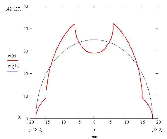
Figure 8: Color online. Probability density function for the CICC calculated with the relations developed in this paper. For reference also the probability density for a simple connected cable is shown.

IV A cable-in-conduit conductor with segregated copper

Next we illustrate the general method to calculate the geometrical probability function for a cable with segregated, discrete copper. Discrete means that the copper wires, which replace some of the superconducting strands, are not dispersed uniformly in the cable cross-section but grouped together in what appears as islands in the cable structure. The geometry, presented in Fig.9 is borrowed from the new advanced $Nb_{3}Sn$ conductor ref5 , a test conductor developed and tested at the SULTAN facility. As can be seen, in the central cable region there are six round copper islands each being a braid of 27 copper wires. The islands are itinerant i.e. rotate in the cross-section as one advance along the cable. As before we define different regions starting from the cable jacket with a radius $r_{c}$. The region 1 is the reference region and we take $\lambda_{1}=1$. The second region is a diluted region due to the circular movement of the copper islands and the dilution factor will be calculated later. The third region is as the first region and we take $\lambda_{3}=1$. Finally, the fourth region is a hole with radius $r_{h}$ and therefore we have here $\rho_{4}=0$ and $\lambda_{4}=0$.

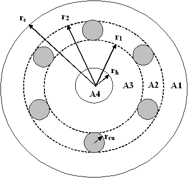
Figure 9: Geometry data for the advanced Nb3Sn cable with six itinerant copper islands and a central hole

In the first region, $r_{2}<|r|<r_{c}$ and we have therefore

$$\begin{array}[]{c}[w(r)]_{1}=\dfrac{\rho_{1}dA_{1}}{\rho_{1}A_{1}+\rho_{2}A_{2}+\rho_{3}A_{3}}=\\ \\ =\dfrac{dA_{1}}{A_{1}+\lambda_{2}A_{2}+A_{3}}\\ \end{array}$$ (39)

Further we have $dA_{1}=2\left(\sqrt{r_{c}^{2}-r^{2}}\right)dr$ and

$$\begin{array}[]{c}A_{1}+\lambda_{2}A_{2}+A_{3}=A_{1}+(A_{2}-A_{2,void})+A_{3}=\\ \\ =A_{1}+A_{2}+A_{3}-A_{2,void}=A-A_{2,void}-A_{4}\\ \end{array}$$ (40)

where $A=\pi r_{c}^{2}$ is the total cable area, $A_{4}=\pi r_{h}^{2}$ the hole area, $A_{2,void}=6\pi r_{Cu}^{2}$ and we used the fact that $A_{1}+A_{2}+A_{3}=A-A_{4}$. Substituting all these in Eq.39 we get

$$[w(r)]_{1}=\dfrac{2\sqrt{r_{c}^{2}-r^{2}}}{A-A_{2,void}-A_{4}}=\dfrac{2\sqrt{r_{c}^{2}-r^{2}}}{A_{eff}}$$ (41)

where in order to simplify the notation we defined $A_{eff}=A-A_{2,void}-A_{4}$.

In the second region, $r_{1}<|r|<r_{2}$ the probability density is

$$[w(r)]_{2}=\dfrac{\rho_{1}dA_{1}+\rho_{2}dA_{2}}{\rho_{1}A_{1}+\rho_{2}A_{2}+\rho_{3}A_{3}}=\dfrac{dA_{1}+\lambda_{2}dA_{2}}{A_{eff}}$$ (42)

and with $dA_{1}=2\left[\sqrt{r_{c}^{2}-r^{2}}-\sqrt{r_{2}^{2}-r^{2}}\right]dr$ and $dA_{2}=2\sqrt{r_{2}^{2}-r^{2}}dr$ we obtain

$$[w(r)]_{2}=\dfrac{2\sqrt{r_{c}^{2}-r^{2}}+2\lambda_{2}\sqrt{r_{2}^{2}-r^{2}}}{A_{eff}}$$ (43)

For the other regions the calculation follows the same scheme and we give here only the final result. For the third and the fourth region we get

$$\begin{array}[]{c}[w(r)]_{3}=\dfrac{2\left[\sqrt{r_{c}^{2}-r^{2}}-\sqrt{r_{2}^{2}-r^{2}}\right]+2\lambda_{2}\left[\sqrt{r_{2}^{2}-r^{2}}-\sqrt{r_{1}^{2}-r^{2}}\right]+2\sqrt{r_{1}^{2}-r^{2}}}{A_{eff}}\\ \\ \left[w(r)\right]_{4}=\dfrac{2\left[\sqrt{r_{c}^{2}-r^{2}}-\sqrt{r_{2}^{2}-r^{2}}\right]+2\lambda_{2}\left[\sqrt{r_{2}^{2}-r^{2}}-\sqrt{r_{1}^{2}-r^{2}}\right]+2\left[\sqrt{r_{1}^{2}-r^{2}}-\sqrt{r_{h}^{2}-r^{2}}\right]}{A_{eff}}\end{array}$$ (44)

The dilution factor for the second region containing the copper islands is

$$\lambda_{2}=1-\dfrac{A_{2,void}}{A_{2}}=1-\dfrac{6\pi r_{Cu}^{2}}{\pi(r_{2}^{2}-r_{1}^{2})}$$ (45)

since the void area is equal to the area of the six copper islands.

The final solution is then of the same form as Eq.38 i.e. a piece-wise continuous function. The result of numerical calculation is shown in Fig.10 and corresponds to the following set of parameters: $r_{h}$=4 mm, $r_{Cu}$=3.25 mm, $r_{1}$=7.85 mm, $r_{2}$=14.35 mm and $r_{c}$=18.2 mm.

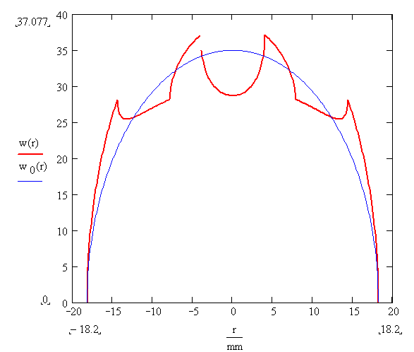
Figure 10: Color online. The probability distribution function for the cable with six copper islands and a central hole

V Conclusions

A method and general relations for calculating the probability distribution function for cable-in-conduit conductors with different geometry have been presented. The probability distribution function is an essential ingredient in the calculation of the average electric field of a cable carrying transport current and exposed to an external uniform magnetic field. This is the only calculation which can be compared with the measured electric field and is an important element in the DC characterization of a cable.

The method was illustrated for two favorite cable geometries with multiple-connected topology. The results of the calculation for a cable with six petals and a central hole and for a cable with six segregated copper islands show that neglecting these geometric aspects could led to large errors in evaluating the average electric field. The central hole is seen to induce a depletion of the probability distribution function in the central region of the cable. Wrapping the last stage results in a depletion close to the jacket and an enhancement close to and around the central hole as illustrated in Fig.8. It is worth mentioning that the depletion in this case occurs at and close to the peak field position. The copper islands effect, Fig.10 is also a depletion but strongly localized around the annulus where the copper segregation is present. The calculation method presented here can be use for almost any type of cable satisfying the ergodic principle.

References

(1) V.I.Arnold and A.Avez,
”Ergodic problems of clasical mechanics”, Redwood City,
California, Addison-Wesley 1989, in the series Advanced book
classics
(2) A.Anghel,
”Self-Field Effect in Large Superconducting Cables for
ITER”, SOFT 21, September 11-15, 2000 Madrid, Spain, published in
Fusion Engineering and Design, 58-59,(2001) 7-11.
(3) J.W.Ekin,
”Strain scaling law and the prediction of uniaxial and
bending strain effects in multifilamentary superconductors”, in
Cryogenic Materials Series, Filamentary A15 Superconductors,
Edited by Masaki Suenaga and Alan F. Clark, Plenum Press New York
and London 1980
(4) N.Mitchell,
”Steady state analysis of non-uniform current distribution
in cable-in-conduit conductors and comparison with experimental
data”, Cryogenics 40, (2000) 99-116
(5) G.Pasztor, P.Bruzzone, A.Anghel and B.Stepanov
”An alternative CICC design aimed at understanding
critical performance issues in Nb3Sn conductors for ITER”,
presented at MT14, 20 October 2003, Morioka, Japan