Exact interacting Green’s function for the Anderson impurity at high bias voltages

Abstract

We describe some exact high-energy properties of a single Anderson impurity connected to two noninteracting leads in a nonequilibrium steady state. In the limit of high bias voltages, and also in the high-temperature limit at thermal equilibrium, the model can be mapped on to an effective non-Hermitian Hamiltonian consisting of two sites, which correspond to the original impurity and its image that is defined in a doubled Hilbert space referred to as Liouville-Fock space. For this, we provide a heuristic derivation using a path-integral representation of the Keldysh contour and the thermal field theory, in which the time evolution along the backward contour is replicated by extra degrees of freedom corresponding to the image. We find that the effective Hamiltonian can also be expressed in terms of charges and currents. From this, it can be deduced that the dynamic susceptibilities for the charges and the current fluctuations become independent of the Coulomb repulsion $U$ in the high bias limit. Furthermore, the equation of motions for the Green’s function and two other higher-order correlation functions constitute a closed system. The exact solution obtained from the three coupled equations extends the atomic-limit solution such that the self-energy correctly captures the imaginary part caused by the relaxation processes at high energies. The spectral weights of the upper and lower Hubbard levels depend sensitively on the asymmetry in the tunneling couplings to the left and right leads.

I Introduction

The impurity Anderson model is one of the most fundamental models for strongly correlated electrons in dilute magnetic alloys,Anderson quantum dots,HDW ; MW and also bulk systems in conjunction with the dynamical mean-field theory.DMFT The model captures essential physics of quantum impurities for the whole energy regions: namely from the formation of a local magnetic moment and the Coulomb blockade occurring at high energies to the low-energy Kondo screening of the local moment.Hewson_book

The Kondo effect has been studied intensively for quantum dots, especially in a nonequilibrium steady state driven by an applied bias voltage.HDW ; MW For instance, the universal Kondo behavior of the steady currentKNG ; ao2001 ; HBA and the shot noiseGogolinKomnik ; Sela2006 ; Golub ; Mora2009 ; Fujii2010 ; Sakano have been shown to be determined by the local-Fermi-liquid parameters for quasiparticles at low energies, where both the bias voltage $eV$ and temperature $T$ are much smaller than the Kondo energy scale $T_{K}$. Low-temperature experiments have also been carried out for the steady currentGrobis ; ScottNatelson and the shot noiseHeiblum ; Kobayashi to examine the universal behavior.

In contrast to the low-energy regions, the properties in the higher energy regions beyond the Fermi-liquid regime have still not been fully understood. In order to explore the intermediate energy regions, numerical approaches such as the Wilson numerical renormalization group,Anders the density matrix renormalization group,Kirino the continuous-time quantum Monte Carlo methods, Werner ; MuhlbacherUrbanKomnik and the Matsubara-voltage approach,Han have been applied. However, analytical approaches, which should be complementary to the numerical ones, are still desired.

In this work, we study the high-energy limit, which is completely opposite to the ground state but is still non-trivial as the Coulomb repulsion $U$ remains competing with the hybridization energy scale $\Delta$. Furthermore, definitive knowledge of the opposite limit is helpful to clarify the nonequilibrium properties of the system for the whole energy regions. Specifically, we consider the high bias limit $eV\to\infty$ where $eV$ is much greater than $T$ and other energy scales of the impurity. In this limit, the model can be mapped exactly onto an effective two-site non-Hermitian Hamiltonian. This can be deduced from an asymptotic form of the Keldysh Green’s function,Keldysh ; Caroli using also a thermal-field-theoretical description.UmeMatTac ; EzaAriHas

We show that the dynamic susceptibilities for the charges, spins, and the current noise, do not depend on $U$ in the high bias limit. More generally, those correlation functions of the operators which commute with the total charge take their noninteracting forms in the limit of $eV\to\infty$. Furthermore, we show that the equation of motion for the Green’s function constitutes a closed system with two other equations of motion for the related higher-order correlation functions. The exact solution in the high bias limit takes an extended form of the well-known atomic-limit solution,HubbardI ; Donianch ; HaugJauho and depends sensitively on the asymmetry in the couplings, $\Gamma_{L}$ and $\Gamma_{R}$, between the impurity and two reservoirs on the left and right, respectively. This asymmetry, which is parameterized by $r\equiv(\Gamma_{L}-\Gamma_{R})/\Delta$ with $\Delta\equiv\Gamma_{L}+\Gamma_{R}$, varies the impurity occupation from half-filling. Furthermore, the self-energy captures a non-trivial imaginary part of the value $3\Delta$ in the denominator. This value of the imaginary part coincides with the corresponding term emerged in the order $U^{2}$ self-energy.AO2002 We also find that the order $U^{2}$ self-energy becomes exact for $\Gamma_{L}=\Gamma_{R}$ in the high bias limit. A similar situation occurs also in the high-temperature limit $T\to\infty$ at thermal equilibrium $eV=0$ without the symmetry between the couplings $\Gamma_{L}$ and $\Gamma_{R}$.AO2002 Namely, in the high-temperature limit, local correlation functions such as the impurity Green’s function do not depend on $r$ and take the same functional forms as those in the symmetric-coupling $\Gamma_{L}=\Gamma_{R}$ case of the high bias limit $eV\to\infty$.

The thermal-field-theoretical approach,UmeMatTac ; EzaAriHas which we will describe in a heuristic way, is equivalent to the Keldysh formalism. This approach may be regarded as a method of images applied to the Hilbert space, and similar formulation has recently been applied to quantum transport problems. EspositeHarolaMukamel ; DzioevKosov ; SaptosovWegewijs In this approach, the degrees of freedoms which correspond to the backward contour in the Keldysh formalism are described by extra operators, defined with respect to a doubled Hilbert space refereed to as Liouville-Fock space. By definition, the extra operators for the enlarged part of the Hilbert space are independent of the original electron operators corresponding to the forward contour. However, a boundary condition is also imposed to the wavefunction at the turnaround point, $t=+\infty$, of the Keldysh contour in order to replicate the linear dependence among the four components of the Keldysh correlation functions.

Our formulation is closely related to that of Saptosov and Wegewijs.SaptosovWegewijs They have pointed out the solvability of the Anderson model in the high-temperature limit $T\to\infty$, where the average occupation of the impurity level is fixed at half-filling, on the basis of an observation that the nonequilibrium reduced density matrix for the impurity site can be constructed exactly by a 16-component supervector with non-Hermitian superoperators defined in the Liouville-Fock space. They have studied in detail the structure of this Hilbert space in the high-temperature limit, by classifying the basis set according to the symmetric properties of some conserved quantities, and have also demonstrated some numerical results for the symmetric couplings $\Gamma_{L}=\Gamma_{R}$.SaptosovWegewijs The 16-component basis apparently corresponds to the two-site degrees of freedom of fermions in our representation. However, the physical back ground which leads some special properties to emerge in the high-energy limit, specifically properties of various correlation functions, still have not been fully clarified.

In this work, we consider the high bias limit $eV\to\infty$, which also has a correspondence to the high-temperature limit as mentioned.AO2002 In general case of the high bias limit, the asymmetry in the couplings $\Gamma_{L}\neq\Gamma_{R}$ varies the average impurity occupation and affects significantly the correlation effects due to $U$. In order to clearly extract the underling physics, we provide a heuristic derivation of the effective two-site Hamiltonian, starting from the path-integral representation of the time evolution along the Keldysh contour. The effective Hamiltonian is non-Hermitian, and can be expressed in terms of charges and currents. Furthermore, the equations of motion for the charges and currents constitute a closed system, in a way that is somewhat similar to the case of the Tomonaga-Luttinger model.GL ; ES We describe these aspects in Sec. II and III. Formulation for the correlation functions is given in Sec. IV. Then, in Sec. V, it is deduced from these equations of motion that the dynamic susceptibilities which conserve the total charge do not depend on $U$ in the high bias limit. It is also the results of this charge and current dynamics that the Green’s function can be deduced exactly from a closed system of the three coupled equations of motion. The exact solution in the high bias limit is compared with the atomic-limit solution in Sec. VI. Summary is given in Sec. VII.

II Keldysh formalism

We start with the single Anderson impurity coupled to two noninteracting leads;

$$\mathcal{H}= \sum_{\sigma}\epsilon_{d,\sigma}\,n_{d\sigma}+U\,n_{d\uparrow}\,n_{d\downarrow}+\!\sum_{\alpha=L,R}\sum_{\sigma}\int_{-D}^{D}\!\!d\epsilon\,\epsilon\,c^{\dagger}_{\epsilon\alpha\sigma}c_{\epsilon\alpha\sigma}$$

$$+\sum_{\alpha=L,R}\sum_{\sigma}v_{\alpha}\left(\psi_{\alpha,\sigma}^{\dagger}d_{\sigma}+d_{\sigma}^{{\dagger}}\psi_{\alpha,\sigma}\right)\;.$$ (1)

Here, $U$ is the Coulomb interaction between the electrons in the quantum dot, and $n_{d\sigma}=d^{{\dagger}}_{\sigma}d_{\sigma}$. The operator $d^{{\dagger}}_{\sigma}$ creates an electron in the quantized level of the energy $\epsilon_{d,\sigma}$ which depends on spin $\sigma$ in the presence of a magnetic field. The operator $c_{\epsilon\alpha\sigma}^{\dagger}$ creates an conduction electron in the lead on the left $\alpha=L$ or right $\alpha=R$ with $\{c^{\phantom{\dagger}}_{\epsilon\alpha\sigma^{\prime}},c^{\dagger}_{\epsilon^{\prime}\alpha^{\prime}\sigma^{\prime}}\}=\delta_{\alpha\alpha^{\prime}}\,\delta_{\sigma\sigma^{\prime}}\delta(\epsilon-\epsilon^{\prime})$. The matrix element $v_{\alpha}$ couples the dot and the lead on $\alpha$ through $\psi_{\alpha\sigma}\equiv\int_{-D}^{D}d\epsilon\sqrt{\rho}\,c^{\phantom{\dagger}}_{\epsilon\alpha\sigma}$, and causes the level broadening $\Delta\equiv\Gamma_{L}+\Gamma_{R}$ with $\Gamma_{\alpha}=\pi\rho\,v_{\alpha}^{2}$ and $\rho=1/(2D)$. We consider the parameter region where the half band-width $D$ is much grater than the other energy scales, $D\gg\max(\Delta,U,|\epsilon_{d,\sigma}|,T,eV)$.

The nonequilibrium steady state, driven by applied bias voltage, can be described by an effective action $\mathcal{S}=\mathcal{S}_{0}+\mathcal{S}_{U}$ for the time evolution in the Keldysh formalism;Keldysh ; Caroli ; MW ; HDW

$$\!\!\mathcal{Z}\,=\,\int\!D\overline{\eta}\,D\eta\ e^{i\,\left[\,\mathcal{S}_{0}(\overline{\eta},\,\eta)\,+\,\mathcal{S}_{U}(\overline{\eta},\,\eta)\,\right]},$$ (2)

$$\!\!\mathcal{S}_{0}\,=\,\sum_{\sigma}\int_{-\infty}^{\infty}dt\,dt^{\prime}\;\overline{\bm{\eta}}_{\sigma}(t)\,\bm{K}_{0,\sigma}(t,t^{\prime})\,\bm{\eta}_{\sigma}(t^{\prime})\;,$$ (3)

$$\!\!\!\mathcal{S}_{U}=-U\!\int\!\!dt\,\Bigl{\{}\,\overline{\eta}_{-,\uparrow}(t)\,\eta_{-,\uparrow}(t)\,\overline{\eta}_{-,\downarrow}(t)\,\eta_{-,\downarrow}(t)$$

$$\qquad\qquad\qquad-\,\overline{\eta}_{+,\uparrow}(t)\,\eta_{+,\uparrow}(t)\,\overline{\eta}_{+,\downarrow}(t)\,\eta_{+,\downarrow}(t)\Bigr{\}}.$$ (4)

Here, $\overline{\bm{\eta}}_{\sigma}=\left(\,\overline{\eta}_{-,\sigma},\,\overline{\eta}_{+,\sigma}\,\right)$ is a pair of the Grassmann numbers for the $-$ and $+$ branches of the Keldysh contour. The kernel $\bm{K}_{0,\sigma}(t,t^{\prime})$ is given by the Fourier transform of the noninteracting Green’s function,

$$\ \quad\bm{K}_{0,\sigma}(t,t^{\prime})\,=\int_{-\infty}^{\infty}\!{d\omega\over 2\pi}\,\left\{\bm{G}_{0,\sigma}(\omega)\right\}^{-1}e^{-i\omega(t-t^{\prime})}\;,$$ (5)

$$\!\!\!\left\{\bm{G}_{0,\sigma}(\omega)\right\}^{-1}=\,(\omega-\epsilon_{d,\sigma})\,\bm{\tau}_{3}-\bm{\Sigma}_{0}(\omega)\;,$$ (6)

$$\qquad\ \bm{\Sigma}_{0}(\omega)\,=\,-i\Delta\bigl{[}\,1-2f_{\mathrm{eff}}(\omega)\,\bigr{]}\bigl{(}\bm{1}-\bm{\tau}_{1}\bigr{)}+\Delta\bm{\tau}_{2}\;.$$ (7)

Here, $\bm{1}$ is the unit matrix and $\bm{\tau}_{j}$ for $j=1,2,3$ are the Pauli matrices,

$$\!\!\!\bm{\tau}_{1}=\left(\begin{matrix}0&1\cr 1&0\cr\end{matrix}\right),\quad\bm{\tau}_{2}=\left(\begin{matrix}0&-i\cr i&\ 0\cr\end{matrix}\right),\quad\bm{\tau}_{3}=\left(\begin{matrix}1&\ 0\cr 0&-1\cr\end{matrix}\right).$$ (8)

The distribution function $f_{\mathrm{eff}}(\omega)$ describes the energy window as shown in Fig. 1, and is defined by

$$f_{\mathrm{eff}}(\omega)\,=\,\frac{\Gamma_{L}\,f_{L}(\omega)+\Gamma_{R}\,f_{R}(\omega)}{\Gamma_{L}+\Gamma_{R}}\;.$$ (9)

Here, $f_{\alpha}(\omega)=[\,e^{(\omega-\mu_{\alpha})/T}+1\,]^{-1}$ and $\mu_{\alpha}$ is the chemical potential for lead $\alpha$. This function $f_{\mathrm{eff}}(\omega)$ also determines the long time behavior of $\bm{K}_{0,\sigma}(t,t^{\prime})$ as a function of $t-t^{\prime}$. Furthermore, the temperature $T$ and bias voltage $eV\equiv\mu_{L}-\mu_{R}$ enter through $f_{\mathrm{eff}}(\omega)$ for the local correlation functions for the impurity site.

Figure 1: The nonequilibrium distribution function $f_{\mathrm{eff}}(\omega)$ for $\mu_{L}-\mu_{R}=eV$ and $T=0$. The Fermi level at equilibrium, $eV=0$, is chosen to be the origin of energy $\omega=0$.

III Liouville-Fock space for $eV\to\infty$

We now consider two kinds of the high-energy limits. One is the high bias limit $eV\gg T$, where $f_{L}\to 1$ and $f_{R}\to 0$. The other is high-temperature limit $T\gg eV$, where $f_{L}=f_{R}\to 1/2$, including thermal equilibrium at $eV=0$ as a special case. In both of the limits, the distribution function $f_{\mathrm{eff}}(\omega)$ becomes a constant independent of the frequency $\omega$,

$$\!\!\!\!\!\!\!\!f_{\mathrm{eff}}(\omega)\,\to\left\{\begin{array}[]{lr}\frac{\Gamma_{L}}{\Gamma_{L}+\Gamma_{R}}\;,&\mbox{for}\ eV\to\infty\\ \quad\frac{1}{2}\quad\ ,&\mbox{for}\ \ \,T\to\infty\rule{0.0pt}{11.38092pt}\end{array}\right.\;,$$ (12)

and then the non-interacting self-energy $\bm{\Sigma}_{0}(\omega)$ also becomes independent of $\omega$. This makes the problems in the high-energy limits solvable. In the following, we concentrate on the $eV\to\infty$ limit because the $T\to\infty$ limit is equivalent to the $\Gamma_{L}=\Gamma_{R}$ case of the $eV\to\infty$ limit as long as the local properties at the impurity site are concerned.

III.1 Effective non-Hermitian Hamiltonian

In this high bias limit, Eq. $\eqref{eq:U0_self_keldysh}$ simplifies in the form

$$\lim_{eV\to\infty}\!\bm{\Sigma}_{0}(\omega)\,=\,\bm{\tau}_{3}\,\bm{L}_{0}\;,$$ (13)

$$\!\!\!\bm{L}_{0}\,\equiv\,i\left[\,\begin{matrix}\Gamma_{L}-\Gamma_{R}&-2\Gamma_{L}\,\cr-2\Gamma_{R}&-(\Gamma_{L}-\Gamma_{R})\rule{0.0pt}{14.22636pt}\cr\end{matrix}\right].$$ (14)

In this limit, the kernel $\bm{K}_{0,\sigma}(t,t^{\prime})$ becomes a short-time function of a Markovian form and vanishes for $t\neq t^{\prime}$. The explicit form contains the $t$ dependence only through the first derivative which arises from the $\omega$ linear part of $\left\{\bm{G}_{0,\sigma}(\omega)\right\}^{-1}$,

$$\!\mathcal{S}_{0}\to\sum_{\sigma}\!\int_{-\infty}^{\infty}\!\!dt\,\bm{\eta}_{\sigma}^{\dagger}(t)\left\{\bm{1}\!\left(\!i\frac{\partial}{\partial t}-\epsilon_{d,\sigma}\!\right)\!-\bm{L}_{0}\right\}\bm{\eta}_{\sigma}(t).$$ (15)

Here, a transformation, $\bm{\eta}_{\sigma}^{\dagger}=\overline{\bm{\eta}}_{\sigma}\,\bm{\tau}_{3}$ keeping the counter part ${\bm{\eta}}_{\sigma}$ unchanged, has been introduced in order to take the time-derivative term diagonal. The interaction part of action $\mathcal{S}_{U}$ does not change the form of Eq. (4) under this transformation,

$$\mathcal{S}_{U}\,=\,-U\!\int\!\!dt\,\Bigl{\{}\,\eta_{-,\uparrow}^{\dagger}(t)\,\eta_{-,\uparrow}(t)\,\eta_{-,\downarrow}^{\dagger}(t)\,\eta_{-,\downarrow}(t)$$

$$\qquad\qquad\qquad\ \ -\,\eta_{+,\uparrow}^{\dagger}(t)\,\eta_{+,\uparrow}(t)\,\eta_{+,\downarrow}^{\dagger}(t)\,\eta_{+,\downarrow}(t)\Bigr{\}}.$$ (16)

Therefore, in the high bias limit, the integrand for the effective action $\mathcal{S}_{0}+\mathcal{S}_{U}$, namely the Lagrangian, does not have an explicit time-dependence other than the first derivative $i\partial/\partial t$ in Eq.  (15).

The effective action of this form can be constructed from a non-Hermitian Hamiltonian which consists of two orbitals; $\,\widehat{H}_{\mathrm{eff}}=\widehat{H}_{\mathrm{eff}}^{(0)}+\widehat{H}_{\mathrm{eff}}^{(U)}$,

$$\widehat{H}_{\mathrm{eff}}^{(0)}= \ \sum_{\sigma}\xi_{d,\sigma}\,Q_{\sigma}\,+\sum_{\sigma}\left(\bm{d}_{\sigma}^{\dagger}\bm{L}_{0}\bm{d}_{\sigma}-i\Delta\right),$$ (17)

$$\widehat{H}_{\mathrm{eff}}^{(U)}= \ U\biggl{[}\Bigl{(}\!n_{-,\uparrow}\!-\!\frac{1}{2}\Bigr{)}\!\Bigl{(}\!n_{-,\downarrow}\!-\!\frac{1}{2}\Bigr{)}\!-\!\Bigl{(}\!n_{+,\uparrow}\!-\!\frac{1}{2}\Bigr{)}\!\Bigl{(}\!n_{+,\downarrow}\!-\!\frac{1}{2}\Bigr{)}\biggr{]}$$

$$= \ U\left(\,Q_{\uparrow}q_{\downarrow}+Q_{\downarrow}q_{\uparrow}\right).$$ (18)

Here, $\xi_{d,\sigma}=\epsilon_{d,\sigma}+U/2$, and ${\bm{d}}_{\sigma}^{\dagger}=\bigl{(}d_{-,\sigma}^{\dagger}\,,\,d_{+,\sigma}^{\dagger}\bigr{)}$ is a set of two independent fermion operators introduced for the $-$ and $+$ branches, respectively. The corresponding charges are defined by $n_{\mu,\sigma}=d_{\mu,\sigma}^{\dagger}d_{\mu,\sigma}$,

$$q_{\sigma}\equiv\frac{n_{-,\sigma}-n_{+,\sigma}}{2},\qquad\ Q_{\sigma}\equiv n_{-,\sigma}+n_{+,\sigma}-1,$$ (19)

and $Q\equiv\sum_{\sigma}Q_{\sigma}$ is the total charge. In this representation, the fermion operators with the label “$-$” describe the original impurity electron $d_{-,\sigma}^{\dagger}\equiv d_{\sigma}^{\dagger}$. The other component with the label “$+$” corresponds to a tilde-conjugate operators $\widetilde{d}_{\sigma}^{\dagger}$ in the standard notation of the thermal field theoryUmeMatTac ; EzaAriHas and is defined in a doubled Hilbert space, which is also referred to as a Liouville-Fock space. EspositeHarolaMukamel ; DzioevKosov ; SaptosovWegewijs Specifically, our representation corresponds to a particle-hole transformed version, in which $\,d_{+,\sigma}^{\dagger}\equiv\widetilde{d}_{\sigma}$.

The time evolution in the doubled Hilbert space can be described by the Heisenberg representation defined with respect to $\widehat{H}_{\mathrm{eff}}$, UmeMatTac ; EzaAriHas

$$\mathcal{O}(t)\,\equiv \ e^{i\widehat{H}_{\mathrm{eff}}t}\,\mathcal{O}\,e^{-i\widehat{H}_{\mathrm{eff}}t}\;,$$ (20)

$$i\,\frac{\partial\mathcal{O}(t)}{\partial t}\,= \ \left[\,\mathcal{O}(t)\,,\,\widehat{H}_{\mathrm{eff}}\,\right]\;.$$ (21)

III.2 Charge and current representation

The Liouville-Fock space for $\widehat{H}_{\mathrm{eff}}$ consists of $4^{2}$ states, which can be classified according to the total charge and spin. One of the meaningful observations on this is that $\widehat{H}_{\mathrm{eff}}$ can be expressed in terms of the charges and currents,

$$\widehat{H}_{\mathrm{eff}}\,= \ \sum_{\sigma}\xi_{d,\sigma}\,Q_{\sigma}+i\sum_{\sigma}\left(P_{\sigma}-\Delta\right),$$ (22)

$$P_{\sigma}\,\equiv \ I_{R,\sigma}+I_{L,\sigma}+2\,\mathcal{W}_{\sigma}\,q_{\sigma},$$ (23)

$$\mathcal{W}_{\sigma}\,\equiv \ (\Gamma_{L}-\Gamma_{R})-i\,\frac{U}{2}\,Q_{\overline{\sigma}}\;.$$ (24)

The Coulomb interaction enters through the last term in the right-hand-side of Eq. (24), where the label $\overline{\sigma}$ for $Q_{\overline{\sigma}}$ denotes the spin opposite to $\sigma$. The operators $I_{R,\sigma}$ and $I_{L,\sigma}$ are defined by

$$I_{R,\sigma}=-2\Gamma_{R}\,d_{+,\sigma}^{\dagger}d_{-,\sigma},\quad\ I_{L,\sigma}=-2\Gamma_{L}\,d_{-,\sigma}^{\dagger}d_{+,\sigma}.$$ (25)

These operators are equivalent to the current flowing from the dot to the right lead and the current flowing from the left lead to the dot, respectively, although they are not Hermitian in the Liouville-Fock space. We find that $Q_{\sigma}$ and $P_{\sigma}$ are conserved, and the equations of motion for the relative charge $q_{\sigma}$ defined in Eq. (19) and the relative current

$$p_{\sigma}\,\equiv\,I_{R,\sigma}-I_{L,\sigma}$$ (26)

consititute a closed system,

$$\frac{\partial Q_{\sigma}}{\partial t}=0,\qquad\quad\frac{\partial P_{\sigma}}{\partial t}=0,$$ (27)

$$\frac{\partial q_{\sigma}}{\partial t}=-\,p_{\sigma},\qquad\frac{\partial p_{\sigma}}{\partial t}=\,4\,\mathcal{L}_{\sigma}^{2}\,q_{\sigma}+2\,\mathcal{W}_{\sigma}P_{\sigma}\;.$$ (28)

Here, the operators $\mathcal{L}_{\sigma}^{2}$ and $\mathcal{W}_{\sigma}$ take complex eigenvalues which depend on the conserved charge $Q_{\overline{\sigma}}$ as

$$\mathcal{L}_{\sigma}^{2}\,\equiv\,\left(\frac{U}{2}\right)^{2}Q_{\overline{\sigma}}^{2}\,+\,i\,(\Gamma_{L}-\Gamma_{R})\,UQ_{\overline{\sigma}}\,-\,\Delta^{2}.$$ (29)

Furthermore, it is deduced from Eqs. (27) and (28) that the second derivative of $p_{\sigma}$ takes a simple form

$$\frac{\partial^{2}p_{\sigma}}{\partial t^{2}}\,= \ -4\,\mathcal{L}_{\sigma}^{2}\,p_{\sigma}\;.$$ (30)

Specifically, in the subspace of $Q_{\overline{\sigma}}=0$, the operator $\mathcal{L}_{\sigma}^{2}$ takes the eigenvalue of $-\Delta^{2}$ that does not depend on the Coulomb interaction. Therefore, the Heisenberg operators for the charges and currents can be expressed simply as a linear combination of $e^{2\Delta t}$ and $e^{-2\Delta t}$, which represent relaxation of a particle-hole pair excitation. Furthermore, due to these properties, the susceptibilities for the charges and currents become independent of the Coulomb interaction in the high bias limit and take the noninteracting forms as it will be discussed in Sec. V. We will also show in Sec. VI that the equations of motion given in Eqs. (27) and (28) also determine essential dynamics of the single-particle Green’s function as well as the fluctuations of the charges and currents.

IV Two reference states: $\langle\!\langle I|\!|$ and $|\!|\rho\rangle\!\rangle$

In this section, we introduce the explicit forms of the final and initial states for the time-dependent perturbation theory in the doubled Hilbert space. These two are also referred to as $\langle\!\langle I|\!|$ and $|\!|\rho\rangle\!\rangle$ in the standard notation of the thermal field theory,UmeMatTac ; EzaAriHas or the Liouville-Fock approaches.EspositeHarolaMukamel ; DzioevKosov ; SaptosovWegewijs Specifically, $\langle\!\langle I|\!|$ is defined such that it satisfies the boundary conditions at $t=+\infty$ while $|\!|\rho\rangle\!\rangle$ includes the information about the statistical distribution. We describe the properties of these two states in the following.

IV.1 Time evolution in the interaction representation

In this subsection, we discuss more in detail the time evolution, which is described in the interaction representation by the operators,

$$\widehat{\mathcal{U}}(t_{2},t_{1})\equiv \ \mathrm{T}\exp\left[-i\displaystyle\int_{t_{1}}^{t_{2}}dt\,e^{i\widehat{H}_{\mathrm{eff}}^{(0)}t}\widehat{H}_{\mathrm{eff}}^{(U)}e^{-i\widehat{H}_{\mathrm{eff}}^{(0)}t}\right],$$ (31)

$$\mathcal{O}^{\mathcal{I}}(t)\,\equiv \ \,e^{i\widehat{H}_{\mathrm{eff}}^{(0)}t}\,\mathcal{O}\,e^{-i\widehat{H}_{\mathrm{eff}}^{(0)}t}\;.$$ (32)

Here, $\mathrm{T}$ in the right-hand side of Eq. (31) is the time-ordering operator.

The unperturbed part of the effective Hamiltonian can be rewritten in a diagonal form

$$\widehat{H}_{\mathrm{eff}}^{(0)}\,= \ \sum_{\sigma}\xi_{d,\sigma}\left(a_{\sigma}^{-1}a_{\sigma}+b_{\sigma}^{-1}b_{\sigma}-1\right)$$

$$\ +\,\sum_{\sigma}\,i\Delta\left(a_{\sigma}^{-1}a_{\sigma}-b_{\sigma}^{-1}b_{\sigma}-1\right)\;.$$ (33)

Here, the operators correspond to the left and right eigenvectors of $\bm{L}_{0}$,

$$\!\!\!a_{\sigma}\equiv\frac{d_{-,\sigma}-d_{+,\sigma}}{\sqrt{2}},\quad a_{\sigma}^{-1}\equiv\frac{\sqrt{2}\bigl{(}\Gamma_{L}d_{-,\sigma}^{\dagger}\!-\Gamma_{R}d_{+,\sigma}^{\dagger}\bigr{)}}{\Gamma_{L}+\Gamma_{R}},$$ (34)

$$\!\!\!b_{\sigma}^{-1}\equiv\frac{d_{-,\sigma}^{\dagger}+\,d_{+,\sigma}^{\dagger}}{\sqrt{2}},\quad b_{\sigma}\equiv\frac{\sqrt{2}\bigl{(}\Gamma_{R}d_{-,\sigma}^{\phantom{|}}\!+\Gamma_{L}d_{+,\sigma}^{\phantom{|}}\bigr{)}}{\Gamma_{L}+\Gamma_{R}}.$$ (35)

These operators satisfy the anti-commutation relations;

$$\!\!\bigl{\{}a_{\sigma},a_{\sigma^{\prime}}^{-1}\bigr{\}}=\bigl{\{}b_{\sigma},b_{\sigma^{\prime}}^{-1}\bigr{\}}=\,\delta_{\sigma\sigma^{\prime}}\;,$$ (36)

$$\!\!\bigl{\{}b_{\sigma},a_{\sigma^{\prime}}^{-1}\bigr{\}}=\bigl{\{}a_{\sigma},b_{\sigma^{\prime}}^{-1}\bigr{\}}=\bigl{\{}a_{\sigma},a_{\sigma^{\prime}\!}\bigr{\}}=\bigl{\{}b_{\sigma},b_{\sigma^{\prime}\!}\bigr{\}}=0.$$ (37)

These operators show different types of long-time behavior in the interaction representation,

$$a_{\sigma}^{\mathcal{I}}(t)=a_{\sigma}e^{(\Delta-i\xi_{d,\sigma})t},\quad\ b_{\sigma}^{\mathcal{I}}(t)=b_{\sigma}e^{-(\Delta+i\xi_{d,\sigma})t}.$$ (38)

This shows that the annihilation operators decay or expand in time depending on the imaginary part of the eigenvalue because of the non-Hermiticy of $\widehat{H}_{\mathrm{eff}}^{(0)}$. Therefore, the final and initial states satisfy a strong requirement that they must describe the relaxation of the correlation functions correctly. We find that such states can be constructed from the left and right eigenstates of doubly-occupied $a_{\sigma}$ particles,

$$\langle\!\langle I|\!|\,\equiv\,\left\langle 0\right|a_{\downarrow}a_{\uparrow}\;,\qquad|\!|\rho\rangle\!\rangle\,\equiv\,a_{\uparrow}^{-1}a_{\downarrow}^{-1}\left|0\right\rangle\;.$$ (39)

One of the reasons is that the components showing an exponential growth can be eliminated only in the case where the propagators are defined with respect to this pair of the states, as

$$\langle\!\langle I|\!|\mathrm{T}\,a^{\mathcal{I}}_{\sigma}(t)\,a^{-1\mathcal{I}}_{\sigma^{\prime}}(0)|\!|\rho\rangle\!\rangle\,= \,-\delta_{\sigma\sigma^{\prime}}\,\theta(-t)\,e^{(\Delta-i\xi_{d,\sigma})t},$$ (40)

$$\langle\!\langle I|\!|\mathrm{T}\,b^{\mathcal{I}}_{\sigma}(t)\,b^{-1\mathcal{I}}_{\sigma^{\prime}}(0)|\!|\rho\rangle\!\rangle\,= \ \ \ \delta_{\sigma\sigma^{\prime}}\,\theta(t)\,e^{-(\Delta+i\xi_{d,\sigma})t}\;.$$ (41)

As a result, these propagators decay for $|t|\to\infty$ properly. We consider the interacting propagators in Sec. IV.3.

The final state $\langle\!\langle I|\!|$, defined in Eq. (39), also satisfies the following relations,

$$\langle\!\langle I|\!|d_{-,\sigma}=\langle\!\langle I|\!|d_{+,\sigma}\;,\qquad\langle\!\langle I|\!|d_{-,\sigma}^{\dagger}=-\langle\!\langle I|\!|d_{+,\sigma}^{\dagger}\;.$$ (42)

These relations are necessary for the construction of the approach and can be regarded as the boundary conditions which replicate the mutual dependence between the $-$ and $+$ components of the Keldysh contour. Furthermore, in the high bias limit, the initial state $|\!|\rho\rangle\!\rangle$ also has similar properties,

$$\Gamma_{L}\,d_{+,\sigma}|\!|\rho\rangle\!\rangle\,= \ -\Gamma_{R}\,d_{-,\sigma}|\!|\rho\rangle\!\rangle\;,$$ (43)

$$\Gamma_{R}\,d_{+,\sigma}^{\dagger}|\!|\rho\rangle\!\rangle\,= \ \ \Gamma_{L}\,d_{-,\sigma}^{\dagger}|\!|\rho\rangle\!\rangle\;.$$ (44)

We see in these relations that the Hamiltonian parameters $\Gamma_{L}$ and $\Gamma_{R}$ appear as the coefficients. These reflect the properties of the density matrix in the limit of $eV\to\infty$, described in the following.

IV.2 Density matrix

The two states $\langle\!\langle I|\!|$ and $|\!|\rho\rangle\!\rangle$, defined in Eq. (39), have some other notable properties: both of them belong to a spin-singlet subspace with the total charge $Q=0$ and are also the eigenstates of $P_{\sigma}$, as

$$\langle\!\langle I|\!|Q_{\sigma}=\,0\;,\qquad\qquad\langle\!\langle I|\!|P_{\sigma}\,=\,\langle\!\langle I|\!|\,\Delta\;,$$ (45)

$$Q_{\sigma}|\!|\rho\rangle\!\rangle\,=\,0\;,\qquad\qquad P_{\sigma}|\!|\rho\rangle\!\rangle\,=\,\Delta\,|\!|\rho\rangle\!\rangle\;.$$ (46)

Furthermore, $\langle\!\langle I|\!|$ and $|\!|\rho\rangle\!\rangle$ are the zero-energy eigenstates of both $\widehat{H}_{\mathrm{eff}}^{(0)}$ and $\widehat{H}_{\mathrm{eff}}$,

$$\langle\!\langle I|\!|\widehat{H}_{\mathrm{eff}}^{(0)}=\,0\;,\qquad\langle\!\langle I|\!|\widehat{H}_{\mathrm{eff}}\,=\,0\;,$$ (47)

$$\widehat{H}_{\mathrm{eff}}^{(0)}|\!|\rho\rangle\!\rangle=\,0\;,\qquad\,\widehat{H}_{\mathrm{eff}}|\!|\rho\rangle\!\rangle\,=\,0\;.$$ (48)

Due to these zero values of the eigenenergies, these two states do not evolve in time,

$$\!\!\!\!\!\langle\!\langle I|\!|\,\widehat{\mathcal{U}}(t,t^{\prime})=\langle\!\langle I|\!|,\quad\ \,|\!|\rho(t)\rangle\!\rangle\equiv\widehat{\mathcal{U}}(t,-\infty)|\!|\rho\rangle\!\rangle=|\!|\rho\rangle\!\rangle.\!\!\!$$ (49)

We consider statistical averages which are defined with respect to $\langle\!\langle I|\!|$ and $|\!|\rho(t)\rangle\!\rangle$ at $t=0$,

$$\langle\mathcal{O}(t)\rangle\equiv\langle\!\langle I|\!|\mathcal{O}(t)|\!|\rho(0)\rangle\!\rangle\ =\ \langle\!\langle I|\!|\mathcal{O}(t)|\!|\rho\rangle\!\rangle\;.$$ (50)

Here, the second equation has been obtained by using Eq. (49). We note that the normalization condition $\langle\!\langle I|\!|\rho\rangle\!\rangle=1$ is satisfied by definition, given in Eq. (39). The underlying statistical weight can be extracted as an Hermitian density matrix, which satisfies $\widehat{\rho}\,|\!|I\rangle\!\rangle=|\!|\rho\rangle\!\rangle$,

$$\widehat{\rho}\,= \,\prod_{\sigma}\bigl{(}\,1+2r\,q_{\sigma}\bigr{)}\;,\qquad\ \ r\equiv\frac{\Gamma_{L}-\Gamma_{R}}{\Gamma_{L}+\Gamma_{R}}\;.$$ (51)

This density matrix for the high bias limit has the properties that the statistical weight does not depend on $U$ but varies as a function of $r$ which parameterizes the asymmetry in the couplings. Specifically, for the symmetric couplings $r=0$, the distribution becomes uniform $\widehat{\rho}=1$.

The average formula, Eq.  (50), reproduces the exact value of the number of the electrons occupied in the dot in the high bias limit [see Appendix A].

$$\langle\!\langle I|\!|n_{-,\sigma}|\!|\rho(0)\rangle\!\rangle\,=\,\frac{\Gamma_{L}}{\Gamma_{L}+\Gamma_{R}}\;,$$ (52)

and $\langle n_{+,\sigma}\rangle=1-\langle n_{-,\sigma}\rangle$. Furthermore, the steady currents through the dot are correctly reproduced and are properly conserved,

$$\!\!\!\!\langle\!\langle I|\!|I_{R,\sigma}|\!|\rho(0)\rangle\!\rangle=\langle\!\langle I|\!|I_{L,\sigma}|\!|\rho(0)\rangle\!\rangle\ =\ \frac{2\Gamma_{L}\Gamma_{R}}{\Gamma_{L}+\Gamma_{R}}\;.$$ (53)

Even in the presence of the Coulomb repulsion $U$, the averages of the charges and currents really take the same values as those in the noninteracting case in the high bias limit, as shown in the Appendix A. The same holds also true for a class of correlation functions, such as the dynamic susceptibilities of charge and currents, as shown in Sec. V.

IV.3 Green’s function for the doubled Hilbert space

In this subsection, we describe the relation between the Green’s function defined with respect to the Liouville-Fock space and the original Keldysh Green’s function. We introduce the noninteracting Green’s function, defined by

$$\mathcal{G}_{0,\sigma}^{\mu\nu}(t)\,\equiv \ -i\,\langle\!\langle I|\!|\mathrm{T}\,d^{\mathcal{I}}_{\mu,\sigma}(t)\,d^{\dagger\mathcal{I}}_{\nu,\sigma}(0)|\!|\rho\rangle\!\rangle\;.$$ (54)

This Green’s function can be calculated by using Eqs. (38) and (39). The result shows a one-to-one correspondence

$$\bm{\mathcal{G}}_{0,\sigma}(t)\equiv\left[\,\begin{matrix}\mathcal{G}^{--}_{0}(t)&\mathcal{G}^{-+}_{0}(t)\cr\mathcal{G}^{+-}_{0}(t)&\mathcal{G}^{++}_{0}(t)\cr\end{matrix}\,\right]\ =\ \bm{G}_{0,\sigma}(t)\,\bm{\tau}_{3}$$ (55)

with the Keldysh Green’s function $\bm{G}_{0,\sigma}$, the explicit form of which in the high bias limit is given by substituting Eq. (13) into Eq. (6) and replacing $\epsilon_{d,\sigma}$ by $\xi_{d,\sigma}$, following the definition of $\widehat{H}_{\mathrm{eff}}^{(0)}$, as

$$\left\{\bm{G}_{0,\sigma}(\omega)\right\}^{-1}=\,\bm{\tau}_{3}\,\Bigl{[}\,(\omega-\xi_{d,\sigma})\bm{1}\,-\,\bm{L}_{0}\,\Bigr{]}\;.$$ (56)

For instance, the retarded Green’s function is given by $G_{0,\sigma}^{r}(t)=-i\theta(t)\,e^{-(\Delta+i\xi_{d,\sigma})t}$ in real time. This explicitly indicates that the dynamics with the non-Hermitian relaxations can be described correctly by the final and initial states defined in Eq. (39).

For interacting case with $U\neq 0$, the full Green’s function in the Liouville-Fock space is defined by

$$\mathcal{G}_{\sigma}^{\mu\nu}(t)\,\equiv \ -i\,\langle\!\langle I|\!|\mathrm{T}\,d^{\phantom{\dagger}}_{\mu,\sigma}(t)\,d^{\dagger}_{\nu,\sigma}(0)|\!|\rho(0)\rangle\!\rangle$$ (57)

$$= \,-i\,\langle\!\langle I|\!|\mathrm{T}\,d^{\mathcal{I}}_{\mu,\sigma}(t)\,d^{\dagger\mathcal{I}}_{\nu,\sigma}(0)\,\widehat{\mathcal{U}}(\infty,-\infty)|\!|\rho\rangle\!\rangle\;.$$ (58)

The same relation between $\bm{\mathcal{G}}_{\sigma}$ and $\bm{G}_{\sigma}$, which is the interacting Keldysh Green’s function, as that in the noninteracting case also holds for $U\neq 0$,

$$\bm{G}_{\sigma}(t)\,= \ \bm{\mathcal{G}}_{\sigma}(t)\,\bm{\tau}_{3}\;.$$ (59)

The Feynman diagrammatic expansion based on the Wick’s theorem is applicable to the interaction representation, Eq. (58), with the final and initial states defined in Eq. (39). The diagrams generated for $\bm{\mathcal{G}}_{\sigma}$ have exact one-to-one correspondence to those for $\bm{G}_{\sigma}$ obtained with the Keldysh perturbation expansion [see Appendix B].

Using the linear dependence among the four components of the Keldysh Green’s function, the retarded and advanced functions can be expressed in the form

$$G_{\sigma}^{r}\,= \ \mathcal{G}_{\sigma}^{--}+\mathcal{G}_{\sigma}^{-+}\,=\,\mathcal{G}_{\sigma}^{+-}+\mathcal{G}_{\sigma}^{++}\;,$$ (60)

$$G_{\sigma}^{a}\,= \ \mathcal{G}_{\sigma}^{--}-\mathcal{G}_{\sigma}^{+-}\,=\,\mathcal{G}_{\sigma}^{++}-\mathcal{G}_{\sigma}^{-+}\;.$$ (61)

In the right-hand side of these two equations, the second equalities for $\mathcal{G}_{\sigma}^{\mu\nu}(t)$’s can also be deduced directly from Eq. (57) using Eq. (42).

It can also be deduced from Eqs. (42)-(44) that each of the four components of $\mathcal{G}_{\sigma}^{\mu\nu}$ can be expressed in terms of $G_{\sigma}^{r}$ and $G_{\sigma}^{a}$ in the limit $eV\to\infty$,

$$\!\!\bm{\mathcal{G}}_{\sigma}(t)\,=\,\frac{G_{\sigma}^{r}(t)}{\Delta}\left[\begin{matrix}\Gamma_{R}&\Gamma_{L}\cr\Gamma_{R}&\Gamma_{L}\rule{0.0pt}{14.22636pt}\cr\end{matrix}\right]+\frac{G_{\sigma}^{a}(t)}{\Delta}\left[\begin{matrix}\ \Gamma_{L}&-\Gamma_{L}\cr-\Gamma_{R}&\ \Gamma_{R}\rule{0.0pt}{14.22636pt}\cr\end{matrix}\right].$$ (62)

This is also one of the properties emerging in the high bias limit, where the density matrix is time independent.

V Charge and current fluctuations

One of the characteristics emerging in the high bias limit is a property of the commutation relation between the unperturbed and perturbed parts of the effective Hamiltonian

$$\left[\,\widehat{H}_{\mathrm{eff}}^{(0)}\,,\,\widehat{H}_{\mathrm{eff}}^{(U)}\,\right]\,=\,iU\left(\,p_{\uparrow}Q_{\downarrow}+p_{\downarrow}Q_{\uparrow}\right)\;.$$ (63)

Specifically, $\widehat{H}_{\mathrm{eff}}^{(U)}$ and $\widehat{H}_{\mathrm{eff}}^{(0)}$ commute in a spin singlet subspace of the total charge $Q=0$, to which both the finial $\langle\!\langle I|\!|$ and the initial $|\!|\rho\rangle\!\rangle$ states belong. This affects significantly the dynamics of the charges and currents which are determined by the system of equations of motion given in Eqs. (27) and (28). The $U$ dependent terms vanish from the equations of motion since the coefficients for the last equation of the four take the noninteracting values $\mathcal{L}_{\sigma}^{2}=-\Delta^{2}$ and $\mathcal{W}_{\sigma}=\Gamma_{L}-\Gamma_{R}$ in the spin singlet subspace with $Q=0$. This is the central reason for the simplifications emerging in the high bias limit.

In order to see this in more detail, we consider the correlation function

$$X_{AB}(t,t^{\prime})\,\equiv \ -i\,\langle\!\langle I|\!|\,\mathrm{T}\,A(t)\,B(t^{\prime})|\!|\rho(0)\rangle\!\rangle\;,$$ (64)

for the operators $A$ and $B$ which commute with the total charge $Q$,

$$\bigl{[}A\,,\,Q\bigr{]}\,=\,\bigl{[}B\,,\,Q\bigr{]}\,=\,0\;.$$ (65)

Furthermore, we assume that both $A$ and $B$ satisfy the conditions:

$$\langle\!\langle I|\!|\bigl{[}\mathcal{O}\,,\,\widehat{H}_{\mathrm{eff}}^{(U)}\bigr{]}\,=\,0\;,\qquad\bigl{[}\mathcal{O}\,,\,\widehat{H}_{\mathrm{eff}}^{(U)}\bigr{]}|\!|\rho\rangle\!\rangle\,=\,0\;,$$ (66)

for $\mathcal{O}=A$ and $B$. One of the most notable properties emerging in the high bias limit is that $X_{AB}(t,t^{\prime})$ is not dependent on $U$. This is because the intermediate state for $X_{AB}(t,t^{\prime})$ between the times $t$ and $t^{\prime}$ also belong to the spin-singlet subspace with $Q=0$ owing to the first condition (65). Furthermore, in this subspace, it is deduced from Eqs. (63) and (66) that $\widehat{H}_{\mathrm{eff}}^{(U)}$ commutes with $A$ and $B$ as well as $\widehat{H}_{\mathrm{eff}}^{(0)}$. Therefore, the correlation function can be rewritten as

$$X_{AB}(t,0)$$

$$\ \ =\,-i\langle\!\langle I|\!|\,\mathrm{T}\,e^{i\widehat{H}_{\mathrm{eff}}^{(0)}t}e^{i\widehat{H}_{\mathrm{eff}}^{(U)}t}Ae^{-i\widehat{H}_{\mathrm{eff}}^{(U)}t}e^{-i\widehat{H}_{\mathrm{eff}}^{(0)}t}\,B|\!|\rho(0)\rangle\!\rangle$$

$$\ \ =\,-i\langle\!\langle I|\!|\,\mathrm{T}\,e^{i\widehat{H}_{\mathrm{eff}}^{(0)}t}Ae^{-i\widehat{H}_{\mathrm{eff}}^{(0)}t}\,B|\!|\rho\rangle\!\rangle\;.$$ (67)

Here, we set $t^{\prime}=0$ for simplicity. The conditions (65) and (66) are satisfied for the charges, currents and also spin operators. Thus, in the limit of $eV\to\infty$, the corresponding susceptibilities take their non-interacting forms, which can also be calculated from a particle-hole bubble in the Keldysh diagrammatic formalism.

V.1 Charge and spin susceptibilities

As an example, we consider the susceptibility for the impurity occupation $\delta n_{\mu,\sigma}\,\equiv\,n_{\mu,\sigma}-\langle n_{\mu,\sigma}\rangle$, which satisfies those conditions given in Eq. (66),

$$\chi^{\mu\nu}_{\sigma\sigma^{\prime}}(t)\,\equiv \ -i\,\mathrm{sign}(\mu)\,\mathrm{sign}(\nu)\,\langle\!\langle I|\!|\,\mathrm{T}\,\delta n_{\mu,\sigma}(t)\,\delta n_{\nu,\sigma^{\prime}}|\!|\rho\rangle\!\rangle$$

$$= \ -i\langle\!\langle I|\!|\,\mathrm{T}\,\delta q_{\sigma}(t)\,\delta q_{\sigma^{\prime}}(0)|\!|\rho\rangle\!\rangle\;.$$ (68)

By definition, each ($\mu$, $\nu$) component of this function is identical to the corresponding Keldysh correlation function with the same label. The factor of $\mathrm{sign}(\mu)$ emerges through a similar way that $\bm{\tau}_{3}$ appears in Eq. (59). The second line of Eq.  (68) can be obtained by using an identity $\delta n_{\mu,\sigma}=\frac{1}{2}\,Q_{\sigma}-\mathrm{sign}(\mu)\,\delta q_{\sigma}$ with $\delta q_{\sigma}\equiv q_{\sigma}-\langle q_{\sigma}\rangle$. As in the case of Eq. (67), $\chi^{\mu\nu}_{\sigma\sigma^{\prime}}(t)$ becomes $U$ independent for $eV\to\infty$ and takes the noninteracting form, the Fourier transform of which is given by

$$\chi^{\mu\nu}_{\sigma\sigma^{\prime}}(\omega)= \ \frac{\Gamma_{L}\Gamma_{R}}{(\Gamma_{L}+\Gamma_{R})^{2}}\left(\frac{1}{\omega+i2\Delta}-\frac{1}{\omega-i2\Delta}\right)\,\delta_{\sigma\sigma^{\prime}}\;.$$ (69)

Here, the value of the imaginary part $2\Delta$ in the denominator is determined by the operator $\mathcal{L}_{\sigma}^{2}$ which takes eigenvalue $-\Delta^{2}$ in this case. As mentioned in Sec. III.2, this eigenvalue causes a $e^{\pm 2\Delta t}$ dependence for the time-evolution of charges and currents through Eq. (30). Alternatively, in the diagrammatic approach this value emerges through the bubble diagram for the particle-hole pair excitation. It gives the total damping rate of $2\Delta$ in the limit of $eV\to\infty$ as a simple sum of the contributions of the particle and the hole parts.

We note that the charge and the spin susceptibilities are given by $\chi^{\mu\nu}_{\uparrow\uparrow}\pm\chi^{\mu\nu}_{\uparrow\downarrow}$. Furthermore, Eq. (69) indicates that all the ($\mu$, $\nu$) components take the same value in the high bias limit, and thus the retarded susceptibilities vanish $\chi^{r}_{\sigma\sigma^{\prime}}\equiv\chi^{--}_{\sigma\sigma^{\prime}}-\chi^{-+}_{\sigma\sigma^{\prime}}\ \to\,0$ in the high bias limit.

V.2 Shot noise

Another important example is the current noise, the spectrum of which can be deduced from the current-current correlation functions (in units of $e^{2}/\hbar$),

$$S_{\alpha\alpha^{\prime}}(\omega)=\int_{-\infty}^{\infty}\!\!dt\,e^{i\omega t}\bigl{[}\langle\delta I_{\alpha}(t)\,\delta I_{\alpha^{\prime}}(0)\rangle+\langle\delta I_{\alpha^{\prime}}(0)\,\delta I_{\alpha}(t)\rangle\bigl{]},$$ (70)

where $\delta I_{\alpha}(t)\equiv\sum_{\sigma}\bigl{[}I_{\alpha,\sigma}(t)-\langle I_{\alpha,\sigma}(t)\rangle\bigr{]}$ denotes the current fluctuations. The current operators commute with the total charge as $\bigl{[}I_{\alpha,\sigma},Q_{\sigma^{\prime}}\bigr{]}=0$. Furthermore, they satisfy the conditions given in Eq. (66) because $\bigl{[}I_{R,\sigma},\widehat{H}_{\mathrm{eff}}^{(U)}\bigr{]}=UQ_{\overline{\sigma}}I_{R,\sigma}$ and $\bigl{[}I_{L,\sigma},\widehat{H}_{\mathrm{eff}}^{(U)}\bigr{]}=-UQ_{\overline{\sigma}}I_{L,\sigma}$. Therefore, the current-current correlation functions are also not affected by the Coulomb interaction in the high bias limit as the one in Eq. (67). Thus, $S_{\alpha\alpha^{\prime}}(\omega)$ also takes the non-interacting form

$$S_{RL}(\omega)= \,\frac{16\Gamma_{L}\Gamma_{R}}{(\Gamma_{L}+\Gamma_{R})^{2}}\ i\left(\frac{\Gamma_{R}^{2}}{\omega+i2\Delta}-\frac{\Gamma_{L}^{2}}{\omega-i2\Delta}\right),$$ (71)

$$S_{LR}(\omega)= \,\frac{16\Gamma_{L}\Gamma_{R}}{(\Gamma_{L}+\Gamma_{R})^{2}}\ i\left(\frac{\Gamma_{L}^{2}}{\omega+i2\Delta}-\frac{\Gamma_{R}^{2}}{\omega-i2\Delta}\right),$$ (72)

$$S_{LL}(\omega)= \left(\frac{4\Gamma_{L}\Gamma_{R}}{\Gamma_{L}+\Gamma_{R}}\right)^{2}(-i)\left(\frac{1}{\omega+i2\Delta}-\frac{1}{\omega-i2\Delta}\right),$$ (73)

and $S_{RR}(\omega)=S_{LL}(\omega)$.

There is one thing that we need to take into account for discussing the current-current correlation functions. In the Liouville-Fock space for the effective Hamiltonian $\widehat{H}_{\mathrm{eff}}$, the operator equivalence between $I_{\alpha,\sigma}$, defined in Eq. (25), and the corresponding original current vertex is sufficient for the off-diagonal components $S_{LR}$ and $S_{RL}$. However, it is not faithful for obtaining the diagonal components corresponding to $S_{LL}$ and $S_{RR}$. This is because those processes which correspond to the bubble diagrams, consisting of the Keldysh Green’s function for the impurity site $\bm{G}_{0,\sigma}$ and that for the isolated lead $\bm{g}_{\alpha}$ as shown in Fig. 2, cannot be described by the operators, $I_{L,\sigma}$ and $I_{R,\sigma}$, projected into the finite Liouville-Fock space for $\widehat{H}_{\mathrm{eff}}$. These processes can be systematically taken into account, using the explicit expression of the current vertecies. These additional contributions to the diagonal components, for the current from the left lead, are given by

$$\widetilde{S}_{LL}(\omega)\,=\,S_{LL}(\omega)+\delta S_{LL}\;,$$ (74)

$$\delta S_{LL}\,=\,\sum_{\sigma}\!\int_{-\infty}^{\infty}\!\frac{d\epsilon}{2\pi}\,v_{L}^{2}$$

$$\qquad\times\Bigl{[}\,g_{L}^{+-}(\epsilon)\,G_{0,\sigma}^{-+}(\epsilon+\omega)+g_{L}^{-+}(\epsilon)\,G_{0,\sigma}^{+-}(\epsilon-\omega)$$

$$\qquad\qquad+g_{L}^{-+}(\epsilon)\,G_{0,\sigma}^{+-}(\epsilon+\omega)+g_{L}^{+-}(\epsilon)\,G_{0,\sigma}^{-+}(\epsilon-\omega)\,\Bigr{]}$$

$$\qquad\xrightarrow{eV\to\infty}\ \ \frac{8\Gamma_{L}\Gamma_{R}}{\Gamma_{L}+\Gamma_{R}}\;.$$ (75)

Here, $g_{L}^{-+}=i2\pi\rho_{L}f_{L}$, and $g_{L}^{+-}=-i2\pi\rho_{L}(1-f_{L})$. The distribution function takes the form $f_{L}(\epsilon)\to 1$ in the limit of $eV\to\infty$. Similarly, for the current to the right lead, we obtain $\widetilde{S}_{RR}(\omega)=S_{RR}(\omega)+\delta S_{RR}$ with $\delta S_{RR}\equiv\delta S_{LL}$. Therefore, the zero-frequency shot noise is given by

$$S_{RL}(0)= \ S_{LR}(0)=\widetilde{S}_{LL}(0)=\widetilde{S}_{RR}(0)$$

$$= \ \frac{4\Gamma_{L}\Gamma_{R}}{\Gamma_{L}+\Gamma_{R}}\,\left(1+r^{2}\right)\ =\ \left(1-r^{4}\right)\Delta\;.$$ (76)

This also agrees with the noninteracting value that can be deduced from the Landauer-type formula in the limit of $eV\to\infty$ [see Appendix A].

 

Figure 2: Feynman diagrams for $\delta S_{LL}$ and $\delta S_{RR}$, which give additional contributions to the diagonal noise spectrum. The solid line denotes the dot Green’s function $G^{\mu\nu}_{0,\sigma}$ and the dashed line denotes that of the isolated lead $g^{\mu\nu}_{\alpha}$ for $\alpha=L,\,R$.

VI Exact Green’s function for $U\neq 0$

In contrast to the correlation functions for the charges and currents discussed above, the Green’s function captures a non-trivial $U$ dependence. This is because the conditions described in Eqs. (65) and (66) do not hold for the single-particle and the single-hole excitations, and the intermediate states belong to the subspace of $Q=1$ and $-1$. We provide in this section the exact interacting Green’s function that is obtained in the high bias limit.

In the limit $eV\to\infty$, all the four components of the Green’s function can be expressed in terms of $G_{\sigma}^{r}$ and $G_{\sigma}^{a}$ as shown in Eq. (62). Furthermore, the advanced function can be obtained from the retarded function through the Fourier transform $G_{\sigma}^{a}(\omega)=\left\{G_{\sigma}^{r}(\omega)\right\}^{*}$. Therefore, we concentrate on the retarded function, which can also expressed in the following form by using Eqs. (42) and (60),

$$G_{\sigma}^{r}(t)\,= \ -i\,\theta(t)\,\langle\!\langle I|\!|\,d_{\mu,\sigma}(t)\,\left(d_{-,\sigma}^{\dagger}+d_{+,\sigma}^{\dagger}\right)|\!|\rho\rangle\!\rangle\;.$$ (77)

Here, the $G_{\sigma}^{r}$ in the left-hand side does not depend on whether the branch $\mu$ for the annihilation operator in the right-hand side is $-$ or $+$ owing to the properties of the final state $\langle\!\langle I|\!|$, shown in Eq. (42).

VI.1 Equations of motion for the retarded functions

The Green’s function can be exactly calculated in the high bias limit from the Heisenberg representation given in Eq. (57), using the Lehmann representation in the finite Liouville-Fock space.SaptosovWegewijs We provide, however, an alternative derivation using the standard equation of motion approach that can easily be compared with the well-known atomic limit solution.HubbardI The equation of motion for $G_{\sigma}^{r}$ can be derived simply by taking a derivative of Eq. (77) with respect to $t$. Then, another correlation function appears through the commutation relation between $d_{\mu,\sigma}$ and $\widehat{H}_{\mathrm{eff}}^{(U)}$. Specifically, in the high bias limit, the dynamics of the charges and currents is determined by the closed system of equations, given in (27) and (28). We find that this also makes the equation of motion for $G_{\sigma}^{r}$ a closed system with two other composite correlation functions of $q_{\overline{\sigma}}(t)$ and $p_{\overline{\sigma}}(t)$, defined by

$$\!\!\!\Phi_{q;\sigma}^{r}(t)\equiv-i\,\theta(t)\langle\!\langle I|\!|\,q_{\overline{\sigma}}(t)\,d_{\mu,\sigma}(t)\!\left(d_{-,\sigma}^{\dagger}\!+d_{+,\sigma}^{\dagger}\right)\!|\!|\rho\rangle\!\rangle,\!$$ (78)

$$\!\!\!\Phi_{p;\sigma}^{r}(t)\equiv-i\,\theta(t)\langle\!\langle I|\!|\,p_{\overline{\sigma}}(t)\,d_{\mu,\sigma}(t)\!\left(d_{-,\sigma}^{\dagger}\!+d_{+,\sigma}^{\dagger}\right)\!|\!|\rho\rangle\!\rangle.\!$$ (79)

Each of these two functions does not depend on whether $\mu=-$ or $+$ in the right-hand side, similarly to $G_{\sigma}^{r}$ shown in Eq. (77). We obtain such a closed system of equations of motion for $G_{\sigma}^{r}$, $\Phi_{q;\sigma}^{r}$ and $\Phi_{p;\sigma}^{r}$, after some straightforward calculations,

$$\left(i\frac{\partial}{\partial t}-\xi_{d,\sigma}+i\Delta\right)G_{\sigma}^{r}(t)-\,U\,\Phi_{q;\sigma}^{r}(t)\,=\ \delta(t)\;,$$ (80)

$$\left(i\frac{\partial}{\partial t}-\xi_{d,\sigma}+i\Delta\right)\Phi_{q;\sigma}^{r}(t)+i\Phi_{p;\sigma}^{r}(t)-\frac{U}{4}G_{\sigma}^{r}(t)\,=\ \frac{1}{2}\,\frac{\Gamma_{L}-\Gamma_{R}}{\Gamma_{L}+\Gamma_{R}}\ \delta(t),$$ (81)

$$\left(i\frac{\partial}{\partial t}-\xi_{d,\sigma}+i\Delta\right)\Phi_{p;\sigma}^{r}(t)\,-\,2\Delta\left[\,\frac{U}{4}\,+\,i(\Gamma_{L}-\Gamma_{R})\,\right]G_{\sigma}^{r}(t)\,+\,i\Bigl{[}\,4\,\Delta^{2}-i\,(\Gamma_{L}-\Gamma_{R})U\,\Bigr{]}\,\Phi_{q;\sigma}^{r}(t)\,=\ 0\;.$$ (82)

This set of equations can be solved by carrying out the Fourier transformation,

$$G_{\sigma}^{r}(\omega)\,= \ \frac{\omega-\xi_{d,\sigma}+i3\Delta+\,r\,\frac{U}{2}}{\mathcal{D}_{\sigma}(\omega)}\;,$$ (83)

$$\Phi_{q;\sigma}^{r}(\omega)\,= \ \frac{1}{4}\,\frac{U+\,2\,r\,(\omega-\xi_{d,\sigma}+i3\Delta)}{\mathcal{D}_{\sigma}(\omega)}\;,$$ (84)

$$\Phi_{p;\sigma}^{r}(\omega)\,= \ \frac{U}{2}\,\frac{\left(1-r^{2}\right)\Delta}{\mathcal{D}_{\sigma}(\omega)}\;.$$ (85)

Here, $\mathcal{D}_{\sigma}(\omega)$ in the denominator is defined by

$$\mathcal{D}_{\sigma}(\omega)=\left(\omega-\xi_{d,\sigma}+i3\Delta\right)\left(\omega-\xi_{d,\sigma}+i\Delta\right)-\frac{U^{2}}{4}-ir\Delta U.$$ (86)

Here, $r$ is the parameter that describes the asymmetry in the couplings as shown in Eq. (51), and $\Delta=\Gamma_{L}+\Gamma_{R}$, as mentioned.

VI.2 Properties of the exact $G_{\sigma}^{r}(\omega)$

We can also deduce the self-energy $\Sigma_{\sigma}^{r}(\omega)$ from Eq. (83), which can be rewritten in a similar form to the atomic-limit solution,

$$G_{\sigma}^{r}(\omega)\,= \ \frac{1}{\omega-\epsilon_{d,\sigma}-\langle n_{d-\sigma}\,\rangle\,U+i\Delta\,-\,\Sigma_{\sigma}^{r}(\omega)}\;,$$ (87)

$$\Sigma_{\sigma}^{r}(\omega)\,= \ \frac{\langle n_{d-\sigma}\rangle\,\bigl{(}1-\langle n_{-\sigma}\rangle\bigr{)}\,U^{2}}{\omega-\epsilon_{d,\sigma}\,-\,\bigl{(}1-\langle n_{d-\sigma}\rangle\bigr{)}\,U+i3\Delta}\;,$$ (88)

where

$$\langle n_{d-\sigma}\rangle\,\equiv\,\frac{\Gamma_{L}}{\Gamma_{L}+\Gamma_{R}}\ =\,\frac{1+r}{2}\;.$$ (89)

The asymmetry in the couplings $r$ varies the impurity occupation from half-filling. We also see that in the high bias limit the self-energy $\Sigma_{\sigma}^{r}(\omega)$ has an imaginary part, $3\Delta$, in the denominator. The original atomic-limit solution does not have such an imaginary part.HubbardI ; Donianch This value, $3\Delta$, corresponds to a sum of the damping rates in the intermediate states, namely $2\Delta$ of virtually excited one particle-hole pair, the propagation of which can be described by Eq. (69), and an additional $\Delta$ of the incident particle (or hole). This value also coincides with the damping rate that one could phenomenologically expect from a Mathiessenn’s rule for systems with a number of independent relaxation processes. In the special case of the symmetric couplings $r=0$, the average impurity occupation is given by $\langle n_{d-\sigma}\rangle=1/2$, and then the exact self-energy takes the same form as that of the order $U^{2}$ results,AO2002 namely $\Sigma_{\sigma}^{r}(\omega)=\left(\frac{U}{2}\right)^{2}/(\omega-\xi_{d,\sigma}+i3\Delta)$. This is also exact for the high-temperature limit of thermal equilibrium, as mentioned.

Figure 3 shows the spectral function, $-\mathrm{Im}\,G_{\sigma}^{r}(\omega)$, for several cases of the asymmetric couplings, choosing $U/(\pi\Delta)=1.0$ and $4.0$. The spectral weight for the upper (lower) Hubbard level increases for $r>0$ ($r<0$) as the asymmetry in the couplings $|r|$ increases. This peak approaches a Lorentzian form with the width $\Delta$ in the limit of $|r|\to 1$. Furthermore, in this figure, the separation of the upper and lower levels is clearly seen for strong interaction $U/(\pi\Delta)=4.0$ while the peak structure is smeared for weak interaction $U/(\pi\Delta)=1.0$. Similarly, for $r<0$, the spectral weight of the lower Hubbard level increases.

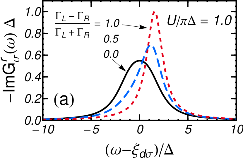
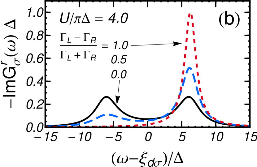
Figure 3: (Color online) Spectral function at $eV\to\infty$ for $U/(\pi\Delta)=1.0$ (a) and $4.0$ (b) for several values of the asymmetric couplings $r\equiv(\Gamma_{L}-\Gamma_{R})/(\Gamma_{L}+\Gamma_{R})$.

The retarded Green’s function, given in Eq. (83), can also be decomposed into the partial fractions,

$$G_{\sigma}^{r}(\omega)\,=\ \frac{Z_{+}}{\omega-\xi_{d,\sigma}+i2\Delta-\mathcal{E}}+\frac{Z_{-}}{\omega-\xi_{d,\sigma}+i2\Delta+\mathcal{E}}\;,$$ (90)

$$Z_{\pm}=\frac{1}{2}\left[1\pm\frac{i\Delta+r\frac{U}{2}}{\mathcal{E}}\right],\quad\,\mathcal{E}\equiv\sqrt{\left(\frac{U}{2}\right)^{2}\!\!-\Delta^{2}+ir\Delta U}.$$ (91)

Here, the complex energy scale $\mathcal{E}$ determines the positions of the poles and its square $\mathcal{E}^{2}$ corresponds to the eigenvalue of the operator $\mathcal{L}_{\overline{\sigma}}^{2}$, defined in Eq.  (29), for $Q_{\sigma}=1$. This energy scale emerges also as an eigenvalue of the effective Hamiltonian.SaptosovWegewijs The complex residues, $Z_{+}$ and $Z_{-}$, represent the contributions of the upper and lower Hubbard levels, which cause two different components emerging in the long-time behavior

$$\!\!\!\!G_{\sigma}^{r}(t)=-i\theta(t)\,e^{-i(\xi_{d,\sigma}-i2\Delta)t}\Bigl{(}Z_{+}\,e^{-i\mathcal{E}t}+Z_{-}\,e^{i\mathcal{E}t}\Bigr{)}.$$ (92)

Therefore, the relaxation time is determined by the imaginary part of the complex energy scale $\mathcal{E}$.SaptosovWegewijs

Figure 4 shows the real and imaginary parts of $\mathcal{E}$ as a function of $U$ for several cases of the asymmetric couplings $r$. The imaginary part of the complex energy is bounded in the range $|\mathrm{Im}\,\mathcal{E}|\leq\Delta$, and thus the relaxation rate of $G_{\sigma}^{r}(t)$ at long time takes the value of $2\Delta-|\mathrm{Im}\,\mathcal{E}|\geq\Delta$. This indicates that the relaxation becomes fast for $U>0$ whereas the asymmetry $|r|$ in the coupling makes relaxation slow. Note that in the noninteracting limit $U\to 0$, the complex energy scale and the residues approach $\mathcal{E}\to i\Delta$, $Z_{+}\to 1$, and $Z_{-}\to 0$. For the symmetric couplings $r=0$, the complex energy scale $\mathcal{E}$ becomes pure imaginary for $U<2\Delta$, and then it becomes real for $U>2\Delta$. The asymmetry in the couplings, $r\neq 0$, makes this sudden change continuous, and $\mathcal{E}$ takes the asymptotic form of $\mathcal{E}\to U/2+i\,r\Delta$ for strong Coulomb repulsion $U\gg\Delta$ while $\mathcal{E}\to|r|\,U/2+i\,\mathrm{sign}(r)\,\Delta$ for weak interactions $U\ll\Delta$. Furthermore, in the limit of $r=\pm 1$, where one of the leads is disconnected, the complex energy scale and the residues takes the values $\mathcal{E}=U/2\pm i\Delta$, $Z_{\pm}=1$, and $Z_{\mp}=0$, respectively.

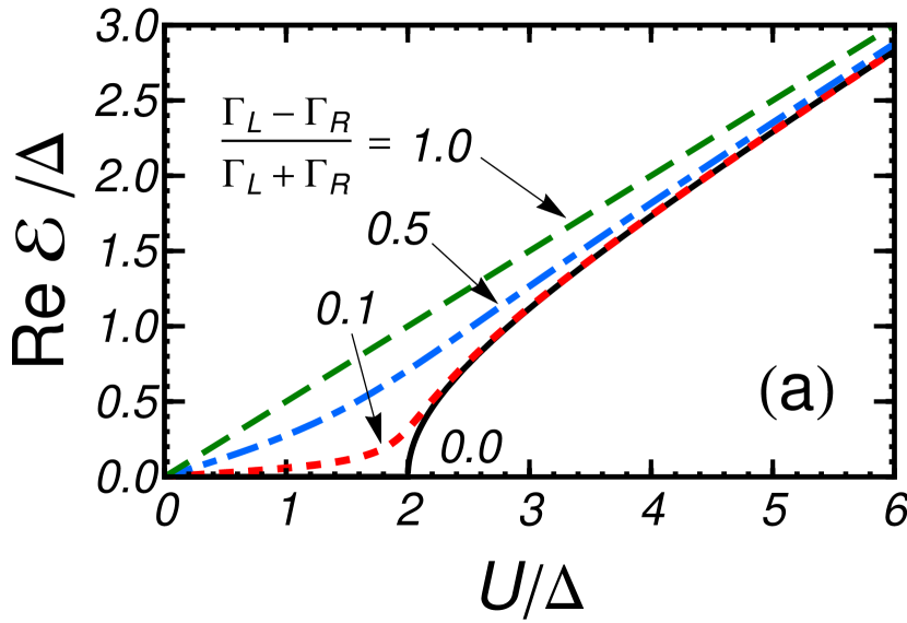
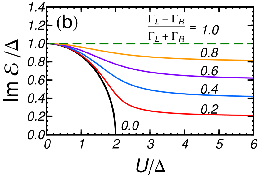
Figure 4: (Color online) $\mathrm{Re}\,\mathcal{E}$ and $\mathrm{Im}\,\mathcal{E}$ of the complex energy scale $\mathcal{E}=\left[\left(U/2\right)^{2}-\Delta^{2}+i\,r\Delta U\right]^{1/2}$ are plotted vs $U$ for several values of $r\equiv(\Gamma_{L}-\Gamma_{R})/(\Gamma_{L}+\Gamma_{R})$ in (a) and (b), respectively.

VII Summary

We have presented the asymptotically exact solutions for the interacting Green’s function and the dynamic correlation functions for the charge, spin and current noise of the Anderson impurity in the high bias limit $eV\to\infty$ of a non-equilibrium steady state.

In this limit, the effective action along the Keldysh contour takes a simplified form because the long-time tail of the kinetic part vanishes, as shown in Eq. (15). This form of the effective action can be replicated by the effective non-Hermitian Hamiltonian $\widehat{H}_{\mathrm{eff}}$, given in Eqs. (17) and (18), with the boundary conditions described in Eqs. (42)–(44). The obtained effective Hamiltonian consists of the two sites, which correspond to the original impurity site and its image, defined with respect to the Liouville-Fock space in the context of the thermal field theory.

It is found that $\widehat{H}_{\mathrm{eff}}$ can be expressed in terms of the charges and currents as Eq. (22). This represents the essential characteristics of the high bias limit, and the equations of motion for the charges and the currents constitute a closed system, given in Eqs. (27) and (28). From this, it is deduced that the dynamic correlation functions for the operators which conserve the total charge become independent of $U$ in the high bias limit as shown in Sec. V.

It is also deduced from the properties of the effective Hamiltonian that all the components of the Keldysh Green’s function are determined by a single element, for instance, by the retarded or advanced Green’s function, as shown in Eq. (62). Furthermore, owing to the characteristics of the charge and current dynamics in the high bias limit, the equations of motion for the retarded Green’s function $G_{\sigma}^{r}$ and the other two high-order correlation functions, $\Phi_{q;\sigma}^{r}$ and $\Phi_{p;\sigma}^{r}$, constitute a closed system, given in Eqs. (80)–(82). The analytic solution for the Green’s function and the self-energy can be expressed in the forms of Eqs. (87) and (88), which can be compared with the atomic-limit solutionHubbardI ; Donianch ; HaugJauho and the order $U^{2}$ results.AO2002 The results show that the self-energy generally captures a non-trivial imaginary part of the value of $3\Delta$ in the denominator in the high bias limit. Furthermore, the asymmetry in the couplings $\Gamma_{L}\neq\Gamma_{R}$ varies the average impurity occupation and affects significantly the correlation effects due to $U$.

Since the seminal work of Hubbard,HubbardI the idea of the atomic limit has been applied and improved in various fields of condensed matter physics. For instance, it has recently been extended to study for quantum dots connected to superconductors. Affleck ; Vecino ; sc2 ; TanakaNQDS ; YsuhiroYamada This work provides a new variety in the atomic-limit approaches. The exact results obtained at the high bias bounds will also be useful to explore further the nonequilibrium properties of quantum impurities in a wide energy range.

Appendix A Some exact results at $eV\to\infty$

Using the usual Keldysh formalism, we show that the impurity occupation and the steady current do not depend on $U$ in the high bias limit. First of all, the impurity occupation can be calculated, for instance, in the following way,Dutt

$$\langle n_{d,\sigma}\rangle\,= \ \int_{-\infty}^{\infty}\frac{d\omega}{2\pi i}\,G_{\sigma}^{-+}(\omega)\,=\,\int_{-\infty}^{\infty}d\omega\,f_{\mathrm{eff}}(\omega)\,A_{\sigma}(\omega)$$

$$\xrightarrow{eV\to\infty} \ \int_{-\infty}^{\infty}d\omega\,\frac{\Gamma_{L}}{\Gamma_{R}+\Gamma_{L}}\,A_{\sigma}(\omega)\ =\ \frac{\Gamma_{L}}{\Gamma_{R}+\Gamma_{L}}\;.$$ (93)

Note that the spectral function $A_{\sigma}(\omega)\equiv\left(-\frac{1}{\pi}\right)\mathrm{Im}\,G_{\sigma}^{r}(\omega)$ satisfies the sum rule $\int_{-\infty}^{\infty}d\omega\,A_{\sigma}(\omega)=1$. Owing to this sum rule, the impurity occupation $\langle n_{d,\sigma}\rangle$ becomes independent of the Coulomb repulsion $U$ and the level position $\epsilon_{d,\sigma}$ in the high bias limit although $A_{\sigma}(\omega)$ varies as a function of $U$ and $\epsilon_{d,\sigma}$. Similarly, in the high bias limit the current $J_{\sigma}$ due to the electrons with spin $\sigma$ can be calculated asMW

$$\!\!\!J_{\sigma}=\frac{e}{\hbar}\int_{-\infty}^{\infty}\!\!\frac{d\omega}{2\pi}\,\bigl{[}\,f_{L}(\omega)-f_{R}(\omega)\,\bigr{]}\,\frac{4\Gamma_{L}\Gamma_{R}}{\Gamma_{L}+\Gamma_{R}}\,\pi A_{\sigma}(\omega)$$

$$\xrightarrow{eV\to\infty}\frac{e}{\hbar}\!\int_{-\infty}^{\infty}\!\!d\omega\,\,\frac{2\Gamma_{L}\Gamma_{R}}{\Gamma_{L}+\Gamma_{R}}\,A_{\sigma}(\omega)=\frac{e}{\hbar}\,\frac{2\Gamma_{L}\Gamma_{R}}{\Gamma_{L}+\Gamma_{R}}.$$ (94)

Here, the factor $e/\hbar$, which was assumed to be $1$ as a unit in the text, is shown explicitly. One can also deduce the high-temperature value of the thermal noise from the linear conductance, using the fluctuation-dissipation theorem,

$$4T\frac{dJ}{dV}\, =\,\frac{e^{2}}{\hbar}\sum_{\sigma}\frac{4\Gamma_{L}\Gamma_{R}}{\Gamma_{L}+\Gamma_{R}}\!\int_{-\infty}^{\infty}\!\!\frac{d\omega}{2\pi}\,4T\left(\!-\frac{\partial f}{\partial\omega}\right)\pi A_{\sigma}(\omega)$$

$$\,\xrightarrow{T\to\infty}\frac{e^{2}}{\hbar}\,\frac{4\Gamma_{L}\Gamma_{R}}{\Gamma_{L}+\Gamma_{R}}\;.$$ (95)

In the noninteracting case $U=0$, the zero-frequency current noise can be expressed in the Landauer-type form

$$\!\!\!\!\!S_{0}(0)\,=\,\frac{e^{2}}{\hbar}\sum_{\sigma}\int\!\frac{d\omega}{2\pi}\ 2\biggl{\{}\,\mathcal{T}_{\sigma}\,\left(\,1-\mathcal{T}_{\sigma}\,\right)\,\left[\,f_{L}\,-\,f_{R}\,\right]^{2}$$

$$\qquad\qquad\quad+\mathcal{T}_{\sigma}\,\bigl{[}\,f_{L}\,(1-f_{L})+(1-f_{R})\,f_{R}\,\bigr{]}\biggr{\}},$$ (96)

$$\!\!\!\!\!\mathcal{T}_{\sigma}(\omega)\,\equiv\,\frac{4\Gamma_{L}\Gamma_{R}}{\left(\omega-\epsilon_{d,\sigma}\right)^{2}+\left(\Gamma_{L}+\Gamma_{R}\right)^{2}}\;.$$ (97)

From this expression, the value of the shot noise in the high bias limit $eV\to\infty$ can be deduced in the form

$$S_{0}(0)\xrightarrow{eV\to\infty} \,\frac{e^{2}}{\hbar}\sum_{\sigma}\int_{-\infty}^{\infty}\!\frac{d\omega}{2\pi}\,2\,\mathcal{T}_{\sigma}\,\left(\,1-\mathcal{T}_{\sigma}\,\right)$$

$$= \ \frac{e^{2}}{\hbar}\,\frac{4\Gamma_{L}\Gamma_{R}}{\Gamma_{L}+\Gamma_{R}}\,\left[\,1+\left(\frac{\Gamma_{L}-\Gamma_{R}}{\Gamma_{L}+\Gamma_{R}}\right)^{2}\,\right].$$ (98)

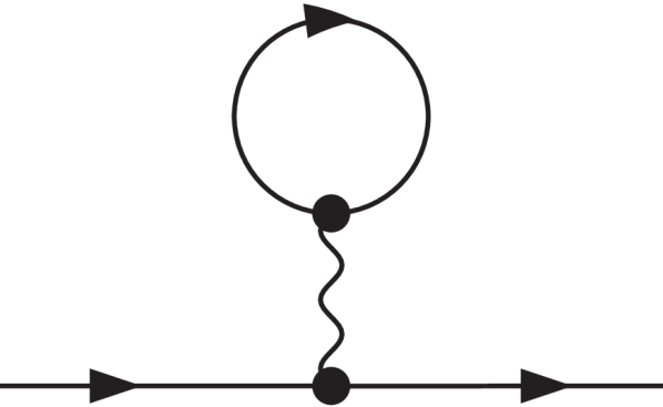
Figure 5: Feynman diagram for the Hartree term.

Appendix B Feynman rule for the Hartree term

There is a slight difference between the Feynman rules for the Keldysh Green’s function $G^{\mu\nu}_{\sigma}$ and those for the Green’s function $\mathcal{G}^{\mu\nu}_{\sigma}$ defined with respect to the doubled Hilbert space. It emerges for the $+$ component of the Hartree-type self-energy $\Sigma^{++}_{\sigma}$, which corresponds to the tadpole diagram shown in Fig. 5. As the arguments $t$ and $t^{\prime}$ for the inner Green’s function along the loop are equal, the limit is required to be taken carefully such that $G^{++}_{\overline{\sigma}}(t+0^{+},t)$ in the Keldysh approach whereas the opposite limit is required for $\mathcal{G}^{++}_{\overline{\sigma}}(t,t+0^{+})$ in the thermal-field-theoretical approach. This is caused by the difference in the direction of the time-ordering for the operators belonging to the $+$ branch. Thus, for the $-$ component of the Hartree-type self-energy $\Sigma^{--}_{\sigma}$, the same limit $t^{\prime}\to t+0^{+}$ is taken for both the Keldysh and the thermal-field-theoretical Green’s functions.

The effective Hamiltonian $\widehat{H}_{\mathrm{eff}}$, defined in Eqs. (17) and (18), includes the $U$-dependent terms such that

$$\frac{U}{2}\sum_{\sigma}Q_{\sigma}\!+\widehat{H}_{\mathrm{eff}}^{(U)}= \ U\left(n_{-,\uparrow}\,n_{-,\downarrow}-n_{+,\uparrow}\,n_{+\downarrow}\right)+\widehat{H}_{\mathrm{eff}}^{(\mathrm{CT})},$$

$$\widehat{H}_{\mathrm{eff}}^{(\mathrm{CT})}\equiv \ U\left(n_{+,\uparrow}+n_{+,\downarrow}-1\right)\;,$$ (99)

Therefore, the last term, $\widehat{H}_{\mathrm{eff}}^{(\mathrm{CT})}$, also appears in the perturbation expansion with respect to $U$ in the thermal-field-theoretical approach. This term can be regarded as a counter term for the particles in the $+$ branch, and compensates the difference that arises in the $+$ component of the Hartree energy shift, mentioned above. We also note that, by definition, the relation between the Keldysh self-energy $\bm{\Sigma}_{\sigma}$ for $\bm{G}_{\sigma}$ and the self-energy $\bm{\mathit{\Sigma}}_{\sigma}^{\mathrm{TFT}}$ for $\bm{\mathcal{G}}_{\sigma}$ can be expressed in the form

$$\bm{\Sigma}_{\sigma}(\omega)\,=\,\bm{\tau}_{3}\,\bm{\mathit{\Sigma}}_{\sigma}^{\mathrm{TFT}}(\omega)\;.$$ (100)

References

- (1) P. W. Anderson, Phys. Rev. 124, 41 (1961).
- (2) S. Hershfield, J. H. Davies, and J. W. Wilkins, Phys. Rev. B 46, 7046 (1992).
- (3) Y. Meir and N. S. Wingreen, Phys. Rev. Lett. 68, 2512 (1992).
- (4) A. Georges, G. Kotliar, W. Krauth, and M. J. Rozenberg, Rev. Mod. Phys. 68, 13 (1996).
- (5) A. C. Hewson, The Kondo Problem to Heavy Fermions (Cambridge University Press, Cambridge, 1993).
- (6) A. Kaminski, Yu. V. Nazarov, and L. I. Glazman, Phys. Rev. B 62, 8154 (2000).
- (7) A. Oguri, Phys. Rev. B 64, 153305 (2001).
- (8) A. C. Hewson, J. Bauer, and A. Oguri, J. Phys.: Condes. Matter. 17, 5413 (2005).
- (9) A. O. Gogolin and A. Komnik, Phys. Rev. B 73, 195301 (2006).
- (10) E. Sela, Y. Oreg, F. von Oppen and J. Koch, Phys. Rev. Lett. 97, 086601 (2006)
- (11) A. Golub, Phys. Rev. B 73, 233310 (2006).
- (12) C. Mora, P. Vitushinsky, X. Leyronas, A. A. Clerk, and K. Le Hur, Phys. Rev. B 80, 155322 (2009).
- (13) T. Fujii, J. Phys. Soc. Jpn. 79, 044714 (2010).
- (14) R. Sakano, T. Fujii, and A. Oguri, Phys. Rev. B 83, 075440 (2011).
- (15) M. Grobis, I. G. Rau, R. M. Potok, H. Shtrikman, and D. Goldhaber-Gordon, Phys. Rev. Lett. 100, 246601 (2008).
- (16) G. D. Scott, Z. K. Keane, J. W. Ciszek, J. M. Tour, and D. Natelson, Phys. Rev. B 79, 165413 (2009).
- (17) O. Zarchin, M. Zaffalon, M. Heiblum, D. Mahalu, and V. Umansky, Phys. Rev. B 77, 241303 (2008).
- (18) Y. Yamauchi, K. Sekiguchi, K. Chida, T. Arakawa, S. Nakamura, K. Kobayashi, T. Ono, T. Fujii, and R. Sakano, Phys. Rev. Lett. 106, 176601 (2011).
- (19) F. B. Anders, Phys. Rev. Lett. 101, 066804 (2008).
- (20) S. Kirino, T. Fujii, J. Zhao, and K. Ueda, J. Phys. Soc. Jpn 77, 084704 (2008).
- (21) P. Werner, T. Oka, and A. J. Millis, Phys. Rev. B 79, 035320 (2009).
- (22) L. Mühlbacher, D. F. Urban, and A. Komnik Phys. Rev. B 83, 075107 (2011).
- (23) J. E. Han, A. Dirks, and T. Pruschke, Phys. Rev. B 86, 155130 (2012).
- (24) L. V. Keldysh, Sov. Phys. JETP 20, 1018 (1965) [Zh. Eksp. Teor. Fiz. 47, 1515 (1964)].
- (25) C. Caroli, R. Combescot, P. Nozieres, and D. Saint-James, J. Phys. C 4, 916 (1971).
- (26) H. Umezawa, H. Matsumoto, and M. Tachiki, Themo Field Dynamics and Condensed States (North-Holland, Amsterdam, 1982).
- (27) H. Ezawa, T. Arimitsu, and Y. Hashimoto, Themal Field Theories (North-Holland, Amsterdam, 1991).
- (28) J. Hubbard, Proc. Roy. Soc. A276, 238 (1963).
- (29) S. Doniach, Adv. Phys. 18, 819 (1969).
- (30) H. Haug and A. -P. Jauho Quantum Kinetics in Transport and Optics of Semiconductors (Springer, Berlin, 1996).
- (31) A. Oguri, J. Phys. Soc. Jpn. 71, 2969 (2002).
- (32) M. Esposite, U. Harbola, and S. Mukamel, Rev. Mod. Phys. 81, 1665 (2009).
- (33) A. A. Dzhioev and D. S. Kosov, J. Chem. Phys. 34, 154107 (2011).
- (34) R. B. Saptsov and M. R. Wegewijs, Phys. Rev. B 86, 235432 (2012).
- (35) Y. Dzyaloshinskii, and A. I. Larkin, Soviet Phys. JETP 38, 202 (1974) [Zh. Eksp. Teor. Fiz. 65, 411 (1973)].
- (36) E. U. Everts and H. Shultz, Solid State Commun. 15, 1413 (1974).
- (37) I. Affleck, J. -S. Caux, and A. M. Zagoskin, Phys. Rev. B 62, 1433 (2000).
- (38) E. Vecino, A. Martin-Rodero, and A. Levy Yeyati, Phys. Rev. B 68, 035105 (2003).
- (39) Yoshihide Tanaka, A. Oguri, and A. C. Hewson, New J. Phys. 9, 115 (2007); 10, 029801(E) (2008).
- (40) Yoichi Tanaka, N. Kawakami, and A. Oguri, J. Phys. Soc. Jpn. 76, 074701 (2007); 77, 098001(E) (2008).
- (41) Yasuhiro Yamada, Yoichi Tanaka, and N. Kawakami, Phys. Rev. B 84, 075484 (2011).
- (42) P. Dutt, J. Koch, J. E. Han, Karyn Le Hur, Ann. Phys. 326, 2963 (2011).