Analytical model of overlapping Feshbach resonances

Abstract

Feshbach resonances in ultracold collisions often result from an interplay between many collision channels. Simple two-channel models can be introduced to capture the basic features, but cannot fully reproduce the situation when several resonances from different closed channels contribute to the scattering process. Using the formalism of multichannel quantum defect theory we develop an analytical model of overlapping Feshbach resonances. We find a general formula for the variation of the scattering length with magnetic field in the vicinity of an arbitrary number of resonances, characterized by simple parameters. Our formula is in excellent agreement with numerical coupled channels calculations for several cases of overlapping resonances in the collisions of two ⁷Li atoms or two Cs atoms.

I Introduction

Magnetically tunable Feshbach resonances have become an essential tool for the control of atomic interactions in ultracold quantum gases Chin et al. (2010). This is because such resonances allow the continuous tuning of the two-body $s$-wave scattering length, a key parameter that controls phenomena such as Bose-Einstein condensation Inouye et al. (1998); Cornish et al. (2000), the crossover physics between Bose-Einstein condensate and Bardeen-Cooper-Schriefer paring in fermonic gases of mixed species Bourdel et al. (2004); Zwierlein et al. (2004), and the formation of weakly bound Feshbach molecules Jochim et al. (2003); Lang et al. (2008). Near the pole position of a resonance at magnetic field $B_{res}$, the scattering length $a(B)$ takes on the following simple form as the field $B$ is varied Moerdijk et al. (1995); Timmermans et al. (1999):

$$a(B)=a_{bg}\left(1-\frac{\Delta}{B-B_{res}}\right)\,,$$ (1)

where $a_{\mathrm{bg}}$ is a constant “background” scattering length in the region of the pole, and $\Delta$ is the width of the resonance; $a(B)=0$ at the “zero crossing” where $B=B_{res}+\Delta$. While scattering lengths are difficult to measure accurately, except for the locations of extreme features such as poles or zero crossings, they can generally be calculated accurately for alkali metal atom species using coupled channels calculations based on models of the ground state potentials Chin et al. (2010). An accurate $a(B)$ function is essential to interpret experiments involving three-body physics, since a key component of the theory is to know the scattering length at the laboratory field $B$ Kraemer et al. (2006); Knoop et al. (2009); Zaccanti et al. (2009); Gross et al. (2010a); Ferlaino et al. (2011); Berninger et al. (2011, 2013); Dyke et al. (2013).

While Eq. (1) is applicable to an isolated single resonance, there are many cases of multiple overlapping resonances, and a generalization to such cases is needed. We derive here an analytic representation of $a(B)$ due to a set of $N$ overlapping resonances from $N$ different closed channels interacting with a single open channel based on the Mies version of multichannel quantum defect theory (MQDT) Mies (1984); Mies and Julienne (1984); Julienne and Mies (1989); Mies and Raoult (2000); Julienne and Gao (2006); Julienne (2009a):

$$a(B)=a_{bg}\left(1-\sum_{i=1}^{N}{\frac{\Delta_{i}}{B-B_{i}-\delta B_{i}-\sum_{j\neq i}{\frac{B-B_{i}}{B-B_{j}}\delta B_{j}}}}\right),$$ (2)

where the sum in the denominator represents a shift due to the mutual interaction of the resonances with the open scattering channel. We will show the connection between this formula and an alternative product form that is based on a square well model of multiple resonances Lange et al. (2009).

This paper will give the MQDT framework for deriving Eq. (2) and illustrate it using fits to coupled channel calculations involving overlapping resonances relevant to the Efimov physics of colliding ⁷Li atoms or Cs atoms. We will discuss how mutual interaction between the resonances affects their positions and local widths. In particular, we will show how a narrow resonance on the shoulder of a broad one can be viewed as a “local” resonance in $B$ with a modified background and width due to the presence of the other resonance.

This work is organized as follows. In Sec. II we briefly review the formulation of MQDT for van der Waals interactions. Sec. III is devoted to derivation and analysis of the formulas describing a single Feshbach resonance using two-channel MQDT theory. In Sec. IV we extend the model to the case of an arbitrary number of closed channels and resulting overlapping resonances. Sec. V contains comparison of our theory to numerical and experimental results as well as characterization of some known resonances in lithium and cesium. Conclusions are drawn in Sec. VI.

II Quantum defect theory.

The collision of two cold atoms, including internal spin degrees of freedom and the effect of short-range forces, can generally be described by a multichannel matrix Schrödinger equation

$$\frac{\partial\mathbf{F(r)}}{\partial r^{2}}+\frac{2\mu}{\hbar^{2}}(E\mathbf{I}-\mathbf{W}(r))\mathbf{F}(r)=0\,,$$ (3)

where $r$, $E$, $\mu$ and $\mathbf{I}$ are respectively the interatomic distance, energy, reduced mass, and the unit matrix. References Köhler et al. (2006); Chin et al. (2010) discuss the various kinds of basis sets that can be used to set up to describe the $(N+1)\times(N+1)$ interaction matrix $\mathbf{W}$ for the collision of two ground S state alkali metal atoms. The number of scattering channels depends on the number of internal spin states of each atom and the number of orbital angular momenta needed to represent the collision. The matrix $\mathbf{W}$ asymptotically approaches a diagonal form

$$W_{ij}\stackrel{{\scriptstyle r\to\infty}}{{\longrightarrow}}\left(E^{\infty}_{i}+\frac{\hbar^{2}\ell_{i}(\ell_{i}+1)}{2\mu r^{2}}-\frac{C_{6}}{r^{6}}\right)\delta_{ij}\,.$$ (4)

Here $\ell_{i}$ is the orbital angular momentum quantum number, $C_{6}$ is the coefficient of the van der Waals potential, and $E^{\infty}_{i}$ is the threshold energy for the $i$th channel. Depending on collision energy $E$, some of the channels can be open ($E>E^{\infty}_{i}$), and some are closed ($E<E^{\infty}_{i}$). Here we assume a single $s$-wave open channel ($\ell=0$).

We start our analysis by a brief review of the MQDT formalism of Mies Mies (1984); Mies and Julienne (1984); Mies and Raoult (2000), which offers some different physical insights than alternative MQDT formalisms Burke et al. (1998); Gao (2008, 2011). Because of the long-range van der Waals potential, we will like Gao Gao (2008, 2011) use $R_{6}=(2\mu C_{6}/\hbar^{2})^{1/4}$ as the unit of length and $E_{6}=\hbar^{2}/2\mu R_{6}^{2}$ as the unit of energy. In MQDT one replaces $\mathbf{W}$ by a set of reference potentials which reproduce the asymptotic form of $\mathbf{W}$ and parameterizes the solution of the new diagonal reference problem at short distances using functions with WKB-like normalization $\hat{f}$, $\hat{g}$. These functions are connected with the long-distance scattering solutions $f$, $g$ (for open channels) or exponentially decaying solutions $\phi$ (for closed channels) using the MQDT functions $C(E)$, $\tan\lambda(E)$ and $\nu(E)$ Julienne and Mies (1989); Mies and Raoult (2000); Julienne (2009a); Idziaszek et al. (2011)

$$\begin{array}[]{lll}f_{i}(r)&=&C_{i}^{-1}(E)\hat{f}_{i}(r)\\ g_{i}(r)&=&C_{i}(E)(\hat{g}_{i}(r)+\tan\lambda_{i}\hat{f}_{i}(r))\\ \phi_{i}(r)&=&\mathcal{N}(E)(\cos\nu_{i}(E)\hat{f}_{i}(r)-\sin\nu_{i}(E)\hat{g}_{i}(r)),\end{array}$$ (8)

where $\mathcal{N}(E)$ ensures unit normalization of the bound state function; see Ref. Julienne (2009a) for a discussion of the normalization of the MQDT functions. Eigenvalues $E_{ni}$ of the reference closed channel $i$ occur where $\tan\nu_{i}(E_{ni})=0$. The general solution of the coupled channels problem can be written as

$$\mathbf{F}(r)=(\mathbf{f}^{0}(r)+\mathbf{Y}\mathbf{g}^{0}(r))\mathbf{A},$$ (9)

where $\mathbf{f}^{0}(r)$ and $\mathbf{g}^{0}(r)$ are diagonal matrices of the reference solutions, $\mathbf{Y}$ is the quantum defect matrix which contains information about the short-range couplings, and $\mathbf{A}$ gives the amplitudes. The short-range processes which determine $\bf{Y}$ are assumed to be present only at length scales $R_{0}\ll R_{6}$. This brings an important simplification to the problem, as the energy scales associated with the short range are much bigger than $E_{6}$, which is of the order of milikelvins. As a result, for ultracold collisions the $\mathbf{Y}$ matrix can be regarded as energy-independent. Moreover, assuming that the potential varies from its long-range form only at short distances makes it possible to use the analytic theory of van der Waals interactions for the MQDT functions Gao (1998, 2000).

The observable properties of the system are given in terms of the open channel block of the scattering matrix $\mathbf{S}$. Within the framework of MQDT, it can be obtained from the quantum defect matrix $\mathbf{Y}$ and the open channel quantum defect functions, as follows Mies (1984):

$$\mathbf{S}_{oo}=e^{i\mathbf{\xi}_{oo}}(1+i\mathbf{R}_{oo})(1-i\mathbf{R}_{oo})^{-1}e^{i\mathbf{\xi}_{oo}},$$ (10)

where $i\mathbf{\xi_{oo}}$ is a diagonal matrix with elements $\xi_{i}\delta_{ij}$ giving the phase shifts for the reference potentials, and

$$\mathbf{R}_{oo}=\mathbf{C}^{-1}(E)(\bar{\mathbf{Y}}_{oo}^{-1}-\tan\mathbf{\lambda}(E)_{oo})^{-1}\mathbf{C}^{-1}(E)\,.$$ (11)

The matrices of the reference channel quantum defect functions $\tan\lambda(E)$, $C(E)$ and $\tan\nu(E)$ are diagonal. The renormalized open channel $\bar{\mathbf{Y}}_{oo}$ matrix is

$$\bar{\mathbf{Y}}_{oo}=\mathbf{Y}_{oo}-\mathbf{Y}_{oc}(\tan\mathbf{\nu}(E)_{cc}+\mathbf{Y}_{cc})^{-1}\mathbf{Y}_{co}\,,,$$ (12)

where the indices $o$ and $c$ respectively denote open and closed channels. Here we assume a single open channel.

III MQDT description of a two-channel resonance.

We will now provide the MQDT description of a single magnetically tunable Feshbach resonance in the simplest case when only one open and one closed channel are present Julienne and Gao (2006). This is general, since Mies et al. Mies et al. (2000) showed how a problem with a single isolated resonance due to multiple closed channels can be reduced to a problem with a single effective closed channel; see also Ref. Nygaard et al. (2006). By choosing the reference potentials to reproduce the true scattering lengths of the uncoupled open and closed channels, the quantum defect matrix $\mathbf{Y}$ will contain only off-diagonal terms

$$\mathbf{Y}=\left(\begin{array}[]{ll}0&y\\ y&0\end{array}\right)\,.$$ (13)

The dimensionless short range coupling parameter $y$ is assumed to be independent of $E$ and $B$. Substituting this into equations (10)-(12), we obtain the $\mathbf{S}_{oo}$ matrix (which in the case of a single open channel is just a complex number $S$) in a factored form with the two factors representing the background and resonant scattering parts:

$$S=e^{2i\xi}\left(1-\frac{2iy^{2}C^{-2}(E)}{\tan\nu(E)+y^{2}\tan\lambda(E)+iy^{2}C^{-2}(E)}\right)\,.$$ (14)

The open reference channel phase shift $\xi\to-ka_{bg}$ as $k\to 0$, and for convenience we choose to write the background scattering length in our $R_{6}$ length units as $a_{bg}=r\bar{a}$, using the mean scattering length of the van der Waals potential, $\bar{a}=2\pi/\Gamma\left(\frac{1}{4}\right)^{2}\approx 0.478$, introduced by Gribakin and Flambaum Gribakin and Flambaum (1993).

The $C^{-2}(E)$ and $\tan\lambda(E)$ functions control the threshold behavior of resonance scattering, giving the respective amplitude and phase relations between the short- and long-range reference functions. Discussion of the physical meaning of these MQDT functions in the cold collision context is given in Refs. Julienne and Mies (1989); Mies and Raoult (2000); Julienne and Gao (2006); Julienne (2009b). When the collision energy $E=\hbar^{2}k^{2}/(2\mu)$ in the open channel becomes large compared to $E_{6}$, then $C^{-2}(E)\to 1$ and $\tan\lambda(E)\to 0$. The threshold behavior for $s$-waves as $E\to 0$ is Mies and Raoult (2000)

$$C^{-2}(E)\to k\bar{a}\left(1+(1-r)^{2}\right),\,\,\,\,\,\tan\lambda(E)\to 1-r\,.$$ (15)

The $\tan\nu(E)$ function in Eq. (14) vanishes at an eigenvalue $E=E_{n}$, where the quantum number $n$ labels the vibrational level. Near such an eigenvalue we can expand the energy-dependence as Mies and Julienne (1984)

$$\tan\nu(E)\approx\left(\frac{\partial\nu}{\partial E}\right)_{E=E_{n}}\left[E-\delta\mu(B-B_{1})\right]$$ (16)

where $E_{n}=\delta\mu(B-B_{1})$ is the field-dependent position of the “bare” closed channel eigenvalue, $\delta\mu$ is the magnetic moment difference between the bare open and closed channel states (measured in $E_{6}$ per gauss units), and $B_{1}$ is the magnetic field at which the bare bound state crosses the open channel threshold. Note that $\pi(\partial E/\partial\nu)_{E_{n}}=\delta E_{n}$ is the mean vibrational spacing near $E=E_{n}$, and $\delta E_{n}/h$ is the corresponding vibrational frequency. If $n$ does not represent the last bound state of the closed channel, a useful approximation is $\delta E_{n}\approx(E_{n+1}-E_{n-1})/2$.

It is straightforward to relate the expression in Eq. (14) to conventional resonant scattering by rewriting the resonant factor as

$$1-\frac{i\hat{\Gamma}C^{-2}(E)}{E-\delta\mu(B-B_{1})+\frac{1}{2}\hat{\Gamma}\tan\lambda(E)+i\frac{1}{2}\hat{\Gamma}C^{-2}(E)}\,,$$ (17)

where

$$\hat{\Gamma}=2y^{2}\left(\frac{\partial E}{\partial\nu}\right)_{E=E_{n}}$$ (18)

is a constant that represents a short-range decay width. Note that the form in Eq. (17) gives the entire $B$-dependence in the $B-B_{1}$ term from the expansion of $\tan\nu(E)$, while the $C(E)^{-2}$ and $\tan\lambda(E)$ MQDT functions give the near-threshold variation with energy. The two terms in the denominator proportional to $\hat{\Gamma}$ represent the energy-dependent shift and width due to the threshold resonance. The numerator of the pole term in Eq. (17) represents the threshold decay width

$$\Gamma(E)=2\pi|\langle\phi_{n}|W_{oc}(r)|f_{o}\rangle|^{2}=\hat{\Gamma}C^{-2}(E)$$ (19)

where $W_{oc}(r)$ is the short-range coupling between the bare open and closed channels. Thus, $\hat{\Gamma}$ represents the width when the open channel scattering wave function $f(r)$ is replaced by the $\hat{f}(r)$ wave function with short range WKB normalization. Following Ref. Mies and Julienne (1984), when $y^{2}\ll 1$ the quantity $4y^{2}$ can be interpreted as the short-range probability that the bound state decays into the open channel during a single vibrational cycle. Multiplying by $C^{-2}(E)$ converts the short-range probability into the proper threshold probability. Consequently, the bare bound state decay rate $\Gamma(E)/\hbar=(4y^{2}C^{-2}(E))(\delta E_{n}/h)$ can be interpreted as the decay probability per cycle times the closed channel vibrational frequency (number of cycles per second).

Simple algebraic transformations of (14) give the energy-dependent scattering length Bolda et al. (2002); Krych and Idziaszek (2009); Idziaszek and Julienne (2010), defined as $\frac{1}{ik}\frac{1-S}{1+S}$, in the form

$$a(E,B)=\frac{C^{-2}y^{2}/k-(\tan\nu+y^{2}\tan\lambda)\tan\xi/k}{\tan\nu+y^{2}\tan\lambda+C^{-2}y^{2}\tan\xi}\,.$$ (20)

By taking the $E\to 0$ limit and making use of relations (16)-(18), we obtain the standard scattering length

$$a(B)=a_{bg}-\frac{\frac{1}{2}\left.\hat{\Gamma}C^{-2}(E)/k\right|_{E\to 0}}{\delta\mu(B-B_{1})-\frac{1}{2}\left.\hat{\Gamma}\tan\lambda(E)\right|_{E\to 0}}\,.$$ (21)

We can now define a resonance width $\Delta$ by writing the “pole strength” in the numerator in Eq. (21) as

$$s_{6}=a_{\mathrm{bg}}\Delta\delta\mu=\frac{1}{2}\hat{\Gamma}C^{-2}(E)/k$$ (22)

Note that the $\Delta$ so defined is the same as in Eq. (22) of Chin et al. Chin et al. (2010); the dimensionless resonance strength parameter defined by Chin et al. Chin et al. (2010) is $s_{\mathrm{res}}=\bar{a}s_{6}\approx 0.478s_{6}$. The $s_{\mathrm{res}}$ (or $s_{6}$) parameter is very important for characterizing the properties of an isolated resonance and also may turn out to be of particular importance in the analysis of three-body recombination near the resonance Wang and Julienne (2013).

With the above definitions, and using the threshold properties in Eq. (15), the $s$-wave scattering length is given by the familiar formula Moerdijk et al. (1995); Timmermans et al. (1999); Chin et al. (2010)

$$a(B)=a_{bg}\left(1-\frac{\Delta}{B-B_{1}-\delta B}\right),$$ (23)

where the width and shift are proportional to $y^{2}$:

$$\Delta = \frac{\delta E_{n}}{\pi\delta\mu}y^{2}\frac{1+(1-r)^{2}}{r}=\frac{s_{6}}{a_{bg}\delta\mu}$$ (24)

$$\delta B = \frac{\delta E_{n}}{\pi\delta\mu}y^{2}(1-r)=\Delta\frac{r(1-r)}{1+(1-r)^{2}}$$ (25)

The latter formula for the shift, previously given in Refs. Köhler et al. (2006); Julienne and Gao (2006); Chin et al. (2010) without derivation, shows that the shift can not be much larger in magnitude than $|\Delta|$, towards which it tends for large $|r|$.

IV Many closed channels.

In many physical systems coupling to a single closed channel is not sufficient to describe the scattering and bound states. In fact, coupled-channels calculations often show many overlapping resonances due to couplings with several closed channels which have poles near one another as a function of $B$ Takekoshi et al. (2012); Berninger et al. (2013); Gross et al. (2011). It is noteworthy that several resonances that have been used to study exotic three-body physics and the Efimov effect occur in regions with overlapping resonances Berninger et al. (2011); Gross et al. (2011). When resonances appear near one another, the simple formula (23) fails to describe the scattering length properly. However, it is straightforward to extend the results from the previous section by adding additional closed channels to the model. We thus start from the quantum defect matrix of the form

$$\mathbf{Y}=\left(\begin{array}[]{llll}0&y_{1}&y_{2}&\ldots\\ y_{1}&0&0&\ldots\\ y_{2}&0&0&\ldots\\ \ldots&\ldots&\ldots&\ldots\end{array}\right).$$ (26)

It is in fact usually not necessary to include couplings between the closed channel states. We can instead assume that we use a basis in which the closed channels are already diagonalised Mies (1968). Then by choosing the reference potentials to reproduce the scattering lengths we get rid of the diagonal terms in the quantum defect matrix as well. As a result of a similar procedure as before and simple algebraic transformations, we obtain the energy-dependent scattering length

$$ka(E)=\frac{C^{-2}\sum_{i}{\frac{y_{i}^{2}}{\tan\nu_{i}}}-\tan\xi\left(1+\tan\lambda\sum_{i}{\frac{y_{i}^{2}}{\tan\nu_{i}}}\right)}{C^{-2}\tan\xi\sum_{i}{\frac{y_{i}^{2}}{\tan\nu_{i}}}+1+\tan\lambda\sum_{i}{\frac{y_{i}^{2}}{\tan\nu_{i}}}}\,,$$ (27)

where the dependence on $B$ is contained in the expansion of each $\tan\nu_{i}(E)$ terms as in Eq. (16). The standard scattering length as $E\to 0$ is

$$a(B)=a_{\mathrm{bg}}-\sum_{i=1}^{N}P_{i}(B)\,.$$ (28)

where the resonant pole terms,

$$P_{i}(B)={\frac{\frac{1}{2}\frac{\hat{\Gamma}_{i}}{\delta\mu_{i}}C^{-2}(E)/k}{B-B_{i}-\frac{1}{2}\tan\lambda(E)\left(\frac{\hat{\Gamma}_{i}}{\delta\mu_{i}}-\sum_{j\neq i}{\frac{B-B_{i}}{B-B_{j}}\frac{\hat{\Gamma}_{j}}{\delta\mu_{j}}}\right)}}\,,$$

imply the $E\to 0$ limit, the widths $\hat{\Gamma}_{i}=2y_{i}^{2}(\delta E_{n\,i}/\pi)$ are defined as in Eq. (18), and $C(E)^{-2}$, $\tan\lambda(E)$, and $r$ are defined for the open channel with background scattering length $a_{bg}$. By defining a resonance width $\Delta_{i}$ and shift $\delta B_{i}$ for each resonance as in Eqs. (22) and (25), we find

$$a(B)=a_{bg}\left(1-\sum_{i}{\frac{\Delta_{i}}{B-B_{i}-\delta B_{i}-\sum_{j\neq i}{\frac{B-B_{i}}{B-B_{j}}\delta B_{j}}}}\right).$$ (29)

The mutual influence of the resonances on one another is thus contained in the terms $\frac{B-B_{i}}{B-B_{j}}\delta B_{j}$. We note that this influence is not due to direct coupling between the closed channels, but rather to indirect interaction via the open channel.

Several important comments are in order here. Firstly, from looking at the structure of Eq. (29) one may suppose that there may be no simple local parameter similar to $s_{res}$ any more, since all the widths are needed to fully describe each resonance. However, it is possible to rewrite Eq. (29) in the form of isolated terms with new parameters, so that it is possible to define a meaningful $s_{res}$ parameter for each resonance. One particularly interesting case is the interplay between a broad resonance and a very narrow one. This is a fairly common situation if a weak resonance of high partial wave character exists near a broad $s$-wave resonance. Assuming two resonances with $\left|\Delta_{1}\right|\ll\left|\Delta_{2}\right|$, Eq. (29) can be simplified to

$$a(B)\approx a_{bg}\left(1-\frac{\Delta_{2}}{B-B^{res}_{2}}-\frac{\alpha\Delta_{1}}{B-B^{res}_{1}}\right),$$ (30)

where $\alpha=\left((B_{1}-B_{2})/(B_{1}-B_{2}-\delta B_{2})\right)^{2}$ renormalizes the width of the narrow resonance and $B^{res}_{i}$ denotes the two pole positions. The new width can be either larger or smaller than $\Delta_{1}$, depending on the background scattering length and the relative position of resonances. One can treat the narrow resonance as an isolated one and describe it by the $s_{res}$ parameter using the renormalized width. By rewriting Eq. (30) as

$$a(B)=a^{\prime}_{bg}\left(1-\frac{\Delta^{\prime}_{1}}{B-B_{1}^{res}}\right)\,,$$ (31)

the scattering length can be approximated as a “local” isolated narrow resonance near $B\approx B_{1}^{res}$ with

$$a^{\prime}_{bg}=a_{bg}\left(1-\frac{\Delta_{2}}{B_{1}^{res}-B_{2}^{res}}\right),\,\,\,\,\Delta^{\prime}_{1}=\frac{\alpha\Delta_{1}}{1-\frac{\Delta_{2}}{B_{1}^{res}-B_{2}^{res}}},$$ (32)

where $s_{6}/\delta\mu_{1}=a^{\prime}_{bg}\Delta^{\prime}_{1}=a_{bg}\alpha\Delta_{1}$ is the same whether the “local” background $a^{\prime}_{bg}$ or “global” background $a_{bg}$ is used.

In general, it is also possible to algebraically transform formula (29) into a product form which was previously derived using a simple model of coupled square wells Lange et al. (2009)

$$a(B)=a_{bg}\prod_{i=1}^{N}{\left(1-\frac{\tilde{\Delta}_{i}}{B-B^{res}_{i}}\right)}.$$ (33)

The transformation can be done by noticing that both (29) and (33) may be represented in the form $a_{bg}\left(1-w_{1}(B)/w_{2}(B)\right)$, where $w_{1}$ and $w_{2}$ are polynomials of $(N-1)$th and $N$th order in $B$. By equating the coefficients in the polynomials one obtains a set of equations connecting both formulas, which can be solved numerically. The resonance positions $B^{res}_{i}$ are given by the zeros of the denominators in (29). However, this usually does not determine the $\tilde{\Delta}$ parameters uniquely. The most “intuitive” solution gives $\tilde{\Delta}_{i}$ as the distance between the pole and the nearest zero of the scattering length, but other solutions are also possible. Consequently, there is no clear interpretation of the $\tilde{\Delta}_{i}$ parameters as resonance widths. Remarkably, each $\tilde{\Delta}_{i}$ and resonance position $B^{res}_{i}$ is a function of all the bare widths $\Delta_{i}$, crossing positions $B_{i}$ and the background scattering length in Eq. (29). Thus, one can always use Eq. (33) to define a pole strength for a “local” pole $i$ as in Eq. (31) as a product of a “local” width $\tilde{\Delta}_{i}$ and a “local” background scattering length,

$$\tilde{a}_{bg,i}=a_{bg}\prod_{j\neq i}^{N}{\left(1-\frac{\tilde{\Delta}_{j}}{B^{res}_{i}-B^{res}_{j}}\right)}\,.$$ (34)

Both $\tilde{a}_{bg,i}$ and $\tilde{\Delta}_{i}$ are functions of all the other pole terms (that is, all the $y_{i}$ parameters), and only their product remains well-determined when the fitting range eliminates distant poles that affect the local region.

Another important question is how to extract multiple resonance parameters by fitting numerical coupled channel calculations of $a(B)$. In some cases, such as ⁷Li in the $f=1,\,m_{f}=0$ spin channel, there are only two resonances Gross et al. (2011), and fitting the formula (29) is relatively easy. In other cases, such as cesium in its $f=3,\,m_{f}=3$ spin channel, the number of resonances is very high Berninger et al. (2013), and the fitting becomes computationally costly. Excluding some resonances from the fitting will matter for the uniqueness of the fit, as Eq. (29) is nonseparable. The effect is larger if any omitted resonances are quite broad or if they lie close to the region of interest. A parameter,

$$\beta_{i}=\frac{\tilde{a}_{bg,i}\tilde{\Delta}_{i}}{a_{bg}\Delta_{i}}\,,$$ (35)

which can be numerically determined by separately fitting $a(B)$ to Eqs. (29) and (33), can be introduced as a measure of the impact of other resonances on the $i$th one. In any case, the product $\tilde{a}_{bg,i}\tilde{\Delta_{i}}$ obtained from the fitting tends to be robust, even if the individual terms are not. Consequently, a meaningful pole strength $\tilde{s}_{6}=\tilde{a}_{bg,i}\tilde{\Delta}_{i}\delta\mu_{i}$ can be defined for each resonance.

Finally, it should be noted that our general formula in Eq. (27) shows how to obtain the scattering properties at finite energies away from $E=0$. Thus, it is more general than the expressions in Eqs.(29) or (33) and can yield effective range or other, more rigorous, finite energy corrections in the presence of single or multiple resonances.

V Applications

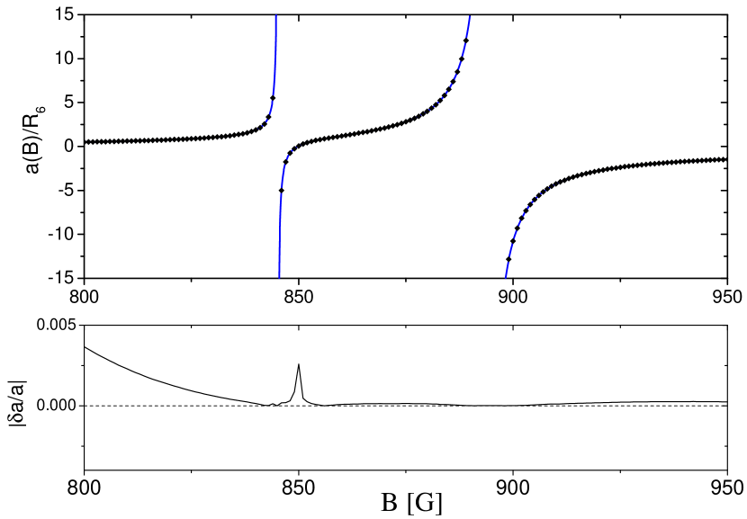
Figure 1: (color online) Top: two $s$-wave Feshbach resonances for the collision of two $f=1,\,m_{f}=0$ ⁷Li atoms. Coupled-channel calculations (black points) compared with the fitted formula (29) (blue line). Bottom: the relative deviation of the fit from the numerical calculations.

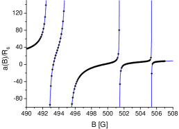
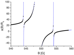
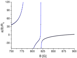
Figure 2: (color online) Some examples of overlapping Feshbach resonances in the collisions of two $f=3,m_{f}=3$ cesium atoms. Left: a structure of four overlapping $d$-wave Feshbach resonances. Middle: a set of two narrow $g$-wave resonances overlapping with a broad $s$-wave one. Right: a broad $s$-wave Feshbach resonance overlapping with a narrow $d$-wave one. Coupled channel calculations Berninger et al. (2013) (black points) are compared with the fit basing on formula (29) (blue lines). The fits are better than $99\%$ accurate in all cases.

Precise Feshbach spectroscopy has been performed for many alkali metal species, and we will use examples of overlapping resonances here that have been studied experimentally for ultracold $f=1,\,m_{f}=0$ ⁷Li Gross et al. (2009, 2011) and $f=3,\,m_{f}=3$ cesium Chin et al. (2004); Berninger et al. (2013). Both of these species have been used in experimental studies of exotic three-body Efimov physics Kraemer et al. (2006); Ferlaino et al. (2011); Berninger et al. (2011); Gross et al. (2009, 2010b, 2011), where it is important to understand the character of the resonances and the mapping of the experimental $B$ field to scattering length. In order to demonstrate in practice how several overlapping resonances can be described, we apply our MQDT formulas to analyze the results of numerical coupled channels calculations using full Hamiltonian models that have been calibrated to reproduce a variety of experimental data. To account for the changing spin character of the channel states at moderate magnetic fields as well as the influence of resonances which were not included in the fit, we allow a small linear variation with $B$ in $a_{bg}(B)=a_{bg}(1+b(B-B_{0}))$ as a first-order correction. We used simple least-square fitting procedures that converge slowly and have to be performed carefully for nonlinear and diverging functions.

Figures 1 and 2 give the results of our fitting. Figure 1 shows the two $s$-wave resonances in collision of two ⁷Li atoms in the $f=1,\,m_{f}=0$ spin channel. For this system the characteristic length $R_{6}\approx 64.973\,a_{0}$ ($a_{0}$ is the Bohr radius) for $C_{6}=$ 1393.39 atomic units Yan et al. (1996) ($E_{\mathrm{h}}a_{0}^{6}$). The coupled channels scattering model was derived from our very accurate model for the collision of ⁶Li atoms Zürn et al. (2013). We fit the binding energy data for the $f=1,\,m_{f}=+1$ ⁷Li spin channel from Ref. Dyke et al. (2013), using a changed scattering length from that of the ⁶Li₂ ${}^{1}\Sigma_{g}^{+}$ potential to account for the failure of isotopic mass scaling, and find coupled channels pole positions at $845.14$ G and $894.00$ G Gau for two $f=1$ ,$m_{f}=1$ atoms, in excellent agreement with the experimental values, 844.9(8) G and 893.7(4) G, reported by Gross et al. Gross et al. (2011). Our least squares fitting of Eq. (29) to a discrete set of coupled channels calculations tabulated on a 1 G grid between 750 G and 950 G yields the same two $B^{res}_{i}$ positions, with $B_{1}=857.08$ G, $B_{2}=828.10$ G, widths $\Delta_{1}=-73.24$ G, $\Delta_{2}=-189.74$ G and the background scattering length $a_{bg}/R_{6}=-0.2339+0.000773(B-800\,G)$ (the definitions ensure that $a_{bg}$ and $\Delta$ have the same sign to fulfill the requirement that $s_{res}$ be positive definite Chin et al. (2010)). These four $B_{i}$ and $\Delta_{i}$ values found are insensitive to the fit range used. Note that $B_{i}$ differs in each case from the pole position $B_{i}^{res}$ because of the large shifts involved. Figure 1 also shows the relative deviation of the fit from the numerics, indicating that the fit quality is better than $99.5\%$ everywhere. A fit of the same quality is obtained if the product form in Eq. (33) is used. Using $\delta\mu\approx 2.66$MHz$/$G, we obtained the $s_{res}$ parameters for these resonances equal to $0.0467$ for the narrow one and $0.493$ for the wide one. Calculating the $\beta$ parameter defined as in Eq. (35) gives $\beta_{1}=0.310$ and $\beta_{2}=1.27$.

In the case of cesium, for which $R_{6}=202.1\,a_{0}$ and $C_{6}=6890.5$ atomic units Berninger et al. (2013), many overlapping resonances in various partial waves (up to the $i$-wave) were observed, and several regions of overlapping resonances are present, some quite complex Berninger et al. (2013). We focus here on three particular regions of magnetic field for which interesting three-body features have also been reported Kraemer et al. (2006); Ferlaino et al. (2011); Berninger et al. (2011). The first is a set of four $d$-wave resonances near $500$ G, the second involves an $s$-wave and two narrow $g$-wave resonances near $550$ G, and finally the third region has an extremely broad $s$-wave resonance near $800$ G with a narrow $d$-wave one on its shoulder not .

Figure 2 shows a comparison of the fits obtained by doing a least-squares fit of Eq. (29) to the coupled channels $a(B)$ function from the Supplemental Material for Ref. Berninger et al. (2013). Table I lists the fitting parameters found using the respective fitting ranges $490$ G to $508$ G, $530$ G to $570$ G, and $750$ G to $900$ G. Note that the background scattering lengths obtained from locally fitting the resonances in each region differ from the global $a_{bg}$, which is expected to be on the order of $\approx 10\,R_{6}$. This means that other resonances not included in the fit are near enough to affect the local background and widths. Nevertheless, the fit quality in all cases stays at the $99\%$ level. A comparable quality fit is obtained by fitting to the product form in Eq. (33). The resonance at $492.7$ G is especially interesting here, as it is broadened by the presence of two stronger ones, that is, its nearby zero-crossing is shifted $0.63$ G from the pole of the resonance. This is consistent with the value of $\beta=$ 12.98, where $\beta$ from Eq. (35) is an analogue of $\alpha$ in Eq. (30) for a narrow resonance affected by two broad ones.

Table I also shows the $s_{res}$ and $\beta$ parameters describing each of the resonances. The $s_{res}$ parameter defined for each resonance is insensitive to fitting ranges. Our respective values of $s_{res}$ of $160$ and $1480$ for the $554.79$ G and $786.83$ G strong $s$-wave resonances compare with the values $170$ and $1470$ estimated by Chin et al. Chin et al. (2010) from an earlier coupled channels model fit to Eq. (1) for a single isolated resonance. The $\beta$ parameter for the broad resonances tend to be the order of unity. However, the narrower resonances on their shoulders show large departures of $\beta$ from unity, implying a renormalization of the pole strength due to interactions among the resonances. We also found that the $554.0$7 G $g$-wave and $820.33$ G $d$-wave resonances, both being narrow ones sitting on the shoulder of the nearby broad $s$-wave one, have respective $s_{res}$ values of 1.6 and 16, differing by an order of magnitude. These $s_{res}$ values are relevant to explaining the three-body physics that has been explored in the vicinity of these resonances Ferlaino et al. (2011); Berninger et al. (2011); Wang and Julienne (2013).

When the formula in Eq. (30) was applied to each of the narrow resonances near $554$ G and $820$ G, with respective $\alpha$ parameters of $\approx$ $0.35$ and $4.5$, the fit quality was only $90\%$ to $95\%$ accurate. However, we found that by using a more complex formula that takes into account the small change in the width of the broad resonance due to its interaction with the narrow ones, we were able to obtain a fit accurate to approximately $99\%$, comparable to that obtained with Eqs. (29) or (33).

$B_{i}^{res}[G]$	$\ell_{i}$	$a_{bg}/R_{6}$	$B_{i}[G]$	$\Delta_{i}$ [G]	$\beta_{i}$	$\delta\mu_{i}/E_{6}$ [G-1]	$s_{res}$
492.68	$d$-wave	$15.2312(1+0.00368(B-500\,G))$	493.315	0.1518	12.98	3.91	56
495.04	$d$-wave	$15.2312(1+0.00368(B-500\,G))$	499.617	3.397	1.05	3.84	100
501.44	$d$-wave	$15.2312(1+0.00368(B-500\,G))$	502.186	2.088	0.093	3.79	5.4
505.38	$d$-wave	$15.2312(1+0.00368(B-500\,G))$	505.483	0.2389	0.194	3.85	1.3
544.19	$g$-wave	$12.7729(1+0.00448(B-550\,G))$	544.108	0.02179	4.95	1.52	1.0
548.79	$s$-wave	$12.7729(1+0.00448(B-550\,G))$	556.693	6.626	1.01	3.90	160
554.07	$g$-wave	$12.7729(1+0.00448(B-550\,G))$	553.793	0.5048	0.387	1.34	1.6
786.17	$s$-wave	$10.7164(1+0.000469(B-800\,G))$	884.638	92.26	0.856	3.66	1480
820.32	$d$-wave	$10.7164(1+0.000469(B-800\,G))$	819.386	0.4508	3.38	2.05	16

Table 1: Resonance parameters obtained from fitting to coupled channels calculations for cesium Berninger et al. (2013) using formula (29). The columns show the position of the resonance $B_{res}$ (magnetic field at which the scattering length diverges), its relevant partial wave $\ell$, the background scattering length $a_{bg}$, magnetic field $B_{i}$ at which the bare bound state crosses the threshold, resonance width $\Delta_{i}$, ratio $\beta_{i}$ from Eq. (35), difference of magnetic moments $\delta\mu_{i}$ (from the coupled channel calculations), and an estimate for $s_{res}\approx 0.478\beta_{i}a_{bg}\Delta_{i}\delta\mu_{i}$.

VI Conclusion

In conclusion, we presented a simple analytical model to describe the variation of the $s$-wave scattering length with magnetic field when there is an arbitrary number of Feshbach resonances. We introduced simple parameters characterizing the system, analogous to the resonance width and background scattering length in the two-channel case. We discussed the non-separability of the scattering length formula for overlapping resonances and provided examples where we accurately reproduced coupled channels numerical results and found the resonance parameters. Apart from characterization of overlapping sets of resonances, our model should be quite helpful for precise mapping of the scattering length to the laboratory $B$ field, which is a critical aspect in the interpretation of experiments with three-body recombination and Efimov physics.

This work was supported by the Foundation for Polish Science International PhD Projects Programme co-financed by the EU European Regional Development Fund, by AFOSR MURI Grant No. FA9550-09-1-0617, and in part by the National Science Foundation under Grant No. NSF PHY11-25915.

References

- Chin et al. (2010) C. Chin, R. Grimm, P. S. Julienne, and E. Tiesinga, Rev. Mod. Phys. 82, 1225 (2010).
- Inouye et al. (1998) S. Inouye, M. R. Andrews, J. Stenger, H.-J. Miesner, D. M. Stamper-Kurn, and W. Ketterle, Nature 392, 151 (1998).
- Cornish et al. (2000) S. L. Cornish, N. R. Claussen, J. L. Roberts, E. A. Cornell, and C. E. Wieman, Phys. Rev. Lett. 85, 1795 (2000).
- Bourdel et al. (2004) T. Bourdel, L. Khaykovich, J. Cubizolles, J. Zhang, F. Chevy, M. Teichmann, L. Tarruell, S. J. J. M. F. Kokkelmans, and C. Salomon, Phys. Rev. Lett. 93, 050401 (2004).
- Zwierlein et al. (2004) M. W. Zwierlein, C. A. Stan, C. H. Schunck, S. M. F. Raupach, A. J. Kerman, and W. Ketterle, Phys. Rev. Lett. 92, 120403 (2004).
- Jochim et al. (2003) S. Jochim, M. Bartenstein, A. Altmeyer, G. Hendl, S. Riedl, C. Chin, J. Hecker Denschlag, and R. Grimm, Science 302, 2101 (2003).
- Lang et al. (2008) F. Lang, K. Winkler, C. Strauss, R. Grimm, and J. Hecker Denschlag, Phys. Rev. Lett. 101, 133005 (2008).
- Moerdijk et al. (1995) A. J. Moerdijk, B. J. Verhaar, and A. Axelsson, Phys. Rev. A 51, 4852 (1995).
- Timmermans et al. (1999) E. Timmermans, P. Tommasini, M. Hussein, and A. Kerman, Phys. Rep. 315, 199 (1999).
- Kraemer et al. (2006) T. Kraemer, M. Mark, P. Waldburger, J. G. Danzl, C. Chin, B. Engeser, A. D. Lange, K. Pilch, A. Jaakkola, H.-C. Nägerl, et al., Nature 440, 315 (2006).
- Knoop et al. (2009) S. Knoop, F. Ferlaino, M. Mark, J. G. Danzl, T. Kraemer, H.-C. Nägerl, and R. Grimm, Nature Phys. 5, 227 (2009).
- Zaccanti et al. (2009) M. Zaccanti, B. Deissler, C. D’Errico, M. Fattori, M. Jona-Lasinio, S. Müller, G. Roati, M. Inguscio, and G. Modugno, Nature Physics 5, 586 (2009).
- Gross et al. (2010a) N. Gross, Z. Shotan, S. Kokkelmans, and L. Khaykovich, Phys. Rev. Lett. 105, 103203 (2010a).
- Ferlaino et al. (2011) F. Ferlaino, A. Zenesini, M. Berninger, B. Huang, H. C. Naegerl, and R. Grimm, Few Body Sys. 51, 113 (2011).
- Berninger et al. (2011) M. Berninger, A. Zenesini, B. Huang, W. Harm, H.-C. Nägerl, F. Ferlaino, R. Grimm, P. S. Julienne, and J. M. Hutson, Phys. Rev. Lett. 107, 120401 (2011).
- Berninger et al. (2013) M. Berninger, A. Zenesini, B. Huang, W. Harm, H.-C. Nägerl, F. Ferlaino, R. Grimm, P. S. Julienne, and J. M. Hutson, Phys. Rev. A 87, 032517 (2013).
- Dyke et al. (2013) P. Dyke, S. E. Pollack, and R. G. Hulet, arXiv:1302.0281 (2013).
- Mies (1984) F. H. Mies, J. Chem. Phys. 80, 2514 (1984).
- Mies and Julienne (1984) F. H. Mies and P. S. Julienne, J. Chem. Phys. 80, 2526 (1984).
- Julienne and Mies (1989) P. S. Julienne and F. H. Mies, J. Opt. Soc. Am. B 6, 2257 (1989).
- Mies and Raoult (2000) F. H. Mies and M. Raoult, Phys. Rev. A 62, 012708 (2000).
- Julienne and Gao (2006) P. S. Julienne and B. Gao, in Atomic Physics 20, edited by C. Roos, H. Häffner, and R. Blatt (AIP, Melville, New York, 2006), pp. 261–268.
- Julienne (2009a) P. S. Julienne, Chapter 6 of Cold Molecules: Theory, Experiment, Applications, ed. by R. V. Krems, W. C. Stwalley, B. Friedrich, CRC Press (arXiv:0902.1727) pp. 221–243 (2009a).
- Lange et al. (2009) A. D. Lange, K. Pilch, A. Prantner, F. Ferlaino, B. Engeser, H.-C. Nägerl, R. Grimm, and C. Chin, Phys. Rev. A 79, 013622 (2009).
- Köhler et al. (2006) T. Köhler, K. Góral, and P. S. Julienne, Rev. Mod. Phys. 78, 1311 (2006).
- Burke et al. (1998) J. P. Burke, C. H. Greene, and J. L. Bohn, Phys. Rev. Lett. 81, 3355 (1998).
- Gao (2008) B. Gao, Phys. Rev. A 78, 012702 (2008).
- Gao (2011) B. Gao, Phys. Rev. A 83, 062712 (2011).
- Idziaszek et al. (2011) Z. Idziaszek, A. Simoni, T. Calarco, and P. S. Julienne, New Journal of Physics 13, 083005 (2011).
- Gao (1998) B. Gao, Phys. Rev. A 58, 1728 (1998).
- Gao (2000) B. Gao, Phys. Rev. A 62, 050702 (2000).
- Mies et al. (2000) F. H. Mies, E. Tiesinga, and P. S. Julienne, Phys. Rev. A 61, 022721 (2000).
- Nygaard et al. (2006) N. Nygaard, B. I. Schneider, and P. S. Julienne, Phys. Rev. A 73, 042705 (2006).
- Gribakin and Flambaum (1993) G. F. Gribakin and V. V. Flambaum, Phys. Rev. A 48, 546 (1993).
- Julienne (2009b) P. S. Julienne, Faraday Discuss. 142, 361 (2009b).
- Bolda et al. (2002) E. L. Bolda, E. Tiesinga, and P. S. Julienne, Phys. Rev. A 66, 013403 (2002).
- Krych and Idziaszek (2009) M. Krych and Z. Idziaszek, Phys. Rev. A 80, 022710 (2009).
- Idziaszek and Julienne (2010) Z. Idziaszek and P. S. Julienne, Phys. Rev. Lett. 104, 113202 (2010).
- Wang and Julienne (2013) Y. Wang and P. S. Julienne, unpublished (2013).
- Takekoshi et al. (2012) T. Takekoshi, M. Debatin, R. Rameshan, F. Ferlaino, R. Grimm, H.-C. Nägerl, C. R. Le Sueur, J. M. Hutson, P. S. Julienne, S. Kotochigova, et al., Phys. Rev. A 85, 032506 (2012).
- Gross et al. (2011) N. Gross, Z. Shotan, O. Machtey, S. Kokkelmans, and L. Khaykovich, Comptes Rendus Phys. 12, 4 (2011).
- Mies (1968) F. H. Mies, Phys. Rev. 175, 164 (1968).
- Gross et al. (2009) N. Gross, Z. Shotan, S. Kokkelmans, and L. Khaykovich, Phys. Rev. Lett. 103, 163202 (2009).
- Chin et al. (2004) C. Chin, V. Vuletić, A. J. Kerman, S. Chu, E. Tiesinga, P. J. Leo, and C. J. Williams, Phys. Rev. A 70, 032701 (2004).
- Gross et al. (2010b) N. Gross, Z. Shotan, S. Kokkelmans, and L. Khaykovich, Phys. Rev. Lett. 105, 103203 (2010b).
- Yan et al. (1996) Z.-C. Yan, J. F. Babb, A. Dalgarno, and G. W. F. Drake, Phys. Rev. A 54, 2824 (1996).
- Zürn et al. (2013) G. Zürn, T. Lompe, A. N. Wenz, S. Jochim, P. S. Julienne, and J. M. Hutson, Phys. Rev. Lett. 110, 135301 (2013).
- (48) Units of gauss rather than tesla, the accepted SI unit for the magnetic field, have been used in this paper to conform to the conventional usage in this field of physics.
- (49) Following the usage of Ref. Chin et al. (2010), an -wave resonance means an -wave bound states is coupled to an -wave open channel.