Time optimization and state-dependent constraints in the quantum optimal control of molecular orientation

Abstract

We apply two recent generalizations of monotonically convergent optimization algorithms to the control of molecular orientation by laser fields. We show how to minimize the control duration by a step-wise optimization and maximize the field-free molecular orientation using state-dependent constraints. We discuss the physical relevance of the different results.

1 Introduction

Optimal control tackles the question of bringing a dynamical system from one state to another with minimum expenditure of time and resources [1, 2]. When applied to quantum systems, control is facilitated by matter wave interference, thus often termed ’coherent control’ [3, 4]. The target state is reached by constructive interference while destructive interference suppresses undesired outcomes. Optimal control has been applied to quantum systems first in the context of physical chemistry to steer chemical reactions [5, 6, 7], followed by control of spin dynamics for applications in NMR [8, 9]. Recently, optimal control is attracting much attention in the context of quantum information processing, for example as a tool to determine the minimum duration of high-fidelity quantum gates [10], and for quantum simulation [11].

For quantum systems with complex dynamics and optimization targets that are difficult to reach, it is impedient to utilize optimal control algorithms that converge fast and monotonically. The core of an optimization algorithm is made up of the control equations which govern the system dynamics and update of the control field. These equations are derived by variation of the target and additional cost functionals. Monotonicity can either be ensured by a smart discretization of the coupled control equations [6, 12, 13] or built in using Krotov’s method [5, 14, 15]. The latter approach comes with the advantage of independence from the specific form of the optimization functional and matter-field interaction [14, 16]. A non-linear matter-field interaction is encountered in multi-photon couplings which are important for example in the control of alignment and orientation [17, 18, 19]. Additional constraints in the optimization functional can be employed to keep the system dynamics within a certain subspace [20] or to restrict the bandwidth of the optimized field [21, 22, 23, 24, 25]. The control time [26, 27, 28, 29] is also a crucial parameter and its optimization can help to avoid, for example, parasitic phenomena with a longer time scale.

The purpose of the present paper is to test the efficiency of two recent optimization procedures, namely state-dependent constraints and time-optimization, when applied to the orientation dynamics of a linear molecule driven by an electromagnetic field. The control of molecular alignment and orientation is by now a well-recognized topic in quantum control with different applications extending from the control of chemical reactions to nanoscale design and quantum computing, see Refs. [30, 31] and references therein. In the past few years, different methods have been proposed to produce molecular orientation such as the use of non-resonant light [32, 33, 34, 35] or THz laser pulses. The latter have the advantage to couple resonantly to the molecular rotational dynamics [36, 37, 38, 39]. It is this option that will be investigated here.

The efficiency of the orientation is one important aspect in view of applications. Another fundamental feature, which has received less attention so far, is the time during which the molecular orientation is above a given threshold under field-free conditions. A standard way to maximize this duration is to restrict the dynamics to a given subspace spanned by the lowest rotational states [40, 41]. Here we study the joint optimization of orientation and its duration, employing the state-dependent constraint algorithm of Ref. [20]. Most of the theoretical and experimental studies have so far been performed in the limit of an isolated molecule where intermolecular collisions are neglected [42, 43]. Dissipative effects such as those due to collisions can be avoided if the optimization time is sufficiently small. We investigate the question of optimization time using the time-optimization algorithm [26, 28, 29], which allows to find the best compromise between the field fluence and the control duration.

The remainder of this paper is organized as follows. The principles of monotonically converging optimal control algorithms are outlined in Sec. 2, with special attention paid to state-dependent constraints and the time-optimization formulation. Section 3 introduces the physical model. The numerical results are presented and discussed in Sec. 4. We conclude in Sec. 5 with an outlook.

2 Review of optimal control algorithms

We present in this section three different optimal control algorithms, considering pure quantum states and assuming the time evolution to be coherent. The formalism is easily extended to mixed states or the control of evolution operators by expanding in a basis [15]. We take the control target to maximize the population of a target state, but modification of the algorithms to maximizing the expectation value of an observable is straightforward. The dynamics of the quantum system is governed by the Hamiltonian

$$H(t)=H_{0}+E(t)H_{1}$$ (1)

with $E(t)$ the control field and $H_{0}$ the field-free Hamiltonian. The operator $H_{1}$ describes the interaction between the system and the control field, which we assume to be linear. We denote the initial and target states by $|\phi_{0}\rangle$ and $|\phi_{f}\rangle$, respectively, and represent a general state by $|\psi(t)\rangle$.

2.1 The standard formulation

We first review the standard formulation of optimal control algorithms with the goal of bringing the system to a target state [5, 6]. The total time $t_{f}$ is fixed. The aim of the control problem is to maximize the cost functional $J$,

$$J[E]=|\langle\psi(t_{f})|\phi_{f}\rangle|^{2}-\lambda\int_{0}^{t_{f}}[E(t)-E_{ref}(t)]^{2}/S(t)dt\,,$$ (2)

where $\lambda$ is a positive parameter which weights the relative importance of the energy of the control field with respect to the projection onto the target state. In Eq. (2), $E_{ref}(t)$ is a reference pulse and $S(t)$ an envelope shape given by $S(t)=\sin^{2}(\pi t/t_{f})$. The function $S(t)$ ensures that the field is smoothly switched on and off at the beginning and at the end of the control. We consider a monotonic optimal control algorithm which allows to increase the cost functional for any choice of the free parameter of the system. More precisely, we determine the field $E_{k+1}$ at step $k+1$ from the field $E_{k}$ at step $k$, such that the variation $\Delta J=J(E_{k+1})-J(E_{k})\geq 0$. At step $k+1$, the reference field $E_{ref}(t)$ is taken to be $E_{k}(t)$ [15]. Then the correction of the control field at step $k+1$ is given by

$$E_{k+1}=E_{k}+\frac{S(t)}{2\lambda}\mathfrak{Im}\left[\langle\chi_{k}|H_{1}|\psi_{k+1}\rangle\right]\,,$$ (3)

where $|\chi_{k}(t)\rangle$ is obtained from backward propagation of the target $|\phi_{f}\rangle$. The dynamics of $|\chi_{k}(t)\rangle$ is governed by the Schrödinger equation just as that for the state of the system $|\psi_{k}(t)\rangle$. The monotonic algorithm for the standard control problem of optimizing state-to-state transfer is summarized as follows:

1. Guess an initial control field for $k=0$ and take $E_{ref}(t)=E_{k}(t)$ at step $k+1$.

2. Propagate forward in time the state of the system $|\psi_{k}\rangle$ with $E_{k}(t)$ from $|\phi_{0}\rangle$.

3. Starting from $|\phi_{f}\rangle\langle\phi_{f}|\psi(t_{f})\rangle$, propagate $|\chi_{k}(t)\rangle$ backward in time with $E_{k}(t)$.

4. Evaluate the correction of the control field, $E_{k+1}-E_{k}$, according to Eq. (3), while propagating the state $|\psi_{k+1}\rangle$ forward in time with $E_{k+1}$, starting from $|\phi_{0}\rangle$.

5. With the new control, $E_{k+1}$, go to step 3 by incrementing the index $k$ by 1.

2.2 State-dependent constraints

Optimal control theory with a state-dependent constraint [20] has been developed in order to restrict the system evolution to a certain subspace. This is useful in order to block multi-photon ionization that can be caused by control fields with high intensity and to avoid subspaces that are subject to decoherence. Formally, optimal control with a state-dependent constraint is equivalent to optimizing a time-dependent target [44, 45]. The corresponding cost functional is expressed as the sum of the functional given in Eq. (2) with a state-dependent intermediate-time cost [20],

$$J^{\mathrm{sdc}}[E]=|\langle\psi(t_{f})|\phi_{f}\rangle|^{2}-\lambda\int_{0}^{t_{f}}[E(t)-E_{ref}]^{2}/S(t)dt+\mu\int_{0}^{t_{f}}\langle\psi(t)|\hat{P}|\psi(t)\rangle dt\,,$$ (4)

where $\mu$ is a positive weight parameter and $\hat{P}$ is here the projector onto the allowed subspace. The control equations which allow for a monotonic increase of the functional, Eq. (4), correspond to those obtained for the standard algorithm modified by an inhomogeneity in the Schrödinger equation for $|\chi_{k}(t)\rangle$, the backward propagated wave function,

$$\frac{\partial}{\partial t}|\chi_{k}(t)\rangle=-i\left[H_{0}+H_{1}E_{k}(t)\right]|\chi_{k}(t)\rangle+\mu\hat{P}|\psi_{k}(t)\rangle\,.$$ (5)

Such an inhomogeneous Schrödinger equation can be solved e.g. by a modified Chebychev propagator [46]. At each iteration $k$, the new control field is given by Eq. (3) with the dynamics of the state $|\psi_{k}(t)\rangle$ governed by the homogeneous Schrödinger equation as before. Other choices for the observable in the intermediate-time cost are possible without perturbing monotonicity of the algorithm, provided the operator is positive or negative semi-definite. This ensures that the sign of the corresponding integral is well-defined [16].

For a state-dependent constraint, the monotonic algorithm is summarized as follows:

1. Guess an initial control field for $k=0$ and take $E_{ref}(t)=E_{k}(t)$ at step $k+1$.

2. Propagate the state of the system, $|\psi_{k}\rangle$, forward in time with $E_{k}$, starting from $|\phi_{0}\rangle$.

3. Evaluate the ’initial’ condition, $|\chi(t_{f})=|\phi_{f}\rangle\langle\phi_{f}|\psi(t_{f})\rangle$, and propagate $|\chi_{k}(t)\rangle$ backward in time with $E_{k}(t)$ by solving the inhomogeneous Schrödinger equation, Eq. (5) [46].

4. Evaluate the correction to the control field, $E_{k+1}-E_{k}$, according to Eq. (3), while propagating the state of the system, $|\psi_{k+1}\rangle$, forward in time with $E_{k+1}$, starting from $|\phi_{0}\rangle$.

5. With the new control, $E_{k+1}$, go to step 3 by incrementing the index $k$ by 1.

2.3 Time optimization

Different formulations of monotonically convergent algorithms with time optimization have been proposed in the literature [26, 28, 29]. Here we follow the approach introduced in Ref. [26] where a cost penalizing both the field fluence and the control duration is used. The cost functional to be maximized can be written as follows:

$$J^{\mathrm{to}}[E]=|\langle\psi(t_{f})|\phi_{f}\rangle|^{2}-\lambda\int_{0}^{t_{f}}[E(t)-E_{ref}(t)]^{2}/S(t)dt\,,$$ (6)

with $t\in[0,t_{f}]$. A rescaling of time $s=t/t_{f}$ leads to normalized quantities independent of $t_{f}$, which will be denoted by a ’tilde’ sign in the following. The new wave function and control field are given by

$$|\tilde{\psi}(s)\rangle=|\psi(st_{f})\rangle\,;\quad\tilde{E}(s)=E(st_{f})\,,$$ (7)

and the cost functional transforms into

$$\tilde{J}^{\mathrm{to}}[\tilde{E};t_{f}]=|\langle\tilde{\psi}(1)|\phi_{f}\rangle|^{2}-\lambda t_{f}\int_{0}^{1}[\tilde{E}(s)-\tilde{E}_{ref}(s)]^{2}/\tilde{S}(s)ds\,.$$ (8)

The goal of the algorithm is now to maximize $\tilde{J}^{\mathrm{to}}$ with respect to $\tilde{E}$ and the time $t_{f}$, which plays here the role of a parameter.

With this new time-parametrization, the wave function $|\tilde{\psi}\rangle$ and the associated adjoint state $|\tilde{\chi}\rangle$ satisfy

$$i\frac{\partial}{\partial s}|\tilde{\psi}(s)\rangle = t_{f}[H_{0}+\tilde{E}(s)H_{1}]|\tilde{\psi}(s)\rangle\,,$$

$$i\frac{\partial}{\partial s}|\tilde{\chi}(s)\rangle = t_{f}[H_{0}+\tilde{E}(s)H_{1}]|\tilde{\chi}(s)\rangle\,.$$

Let us assume that at step $k$ of the iterative algorithm the system is described by the quadruplet $\left(|\tilde{\psi}_{k}\rangle,|\tilde{\chi}_{k}\rangle,\tilde{E}_{k},t_{f}^{(k)}\right)$. We determine the quadruplet at step $k+1$ from the one at step $k$ by the following operations, which are decomposed into two substeps. We first fix the time parameter $t_{f}^{(k)}$ and optimize the control field by a standard algorithm, as the one described in Sec. 2.1. We then get a new quadruplet $\left(|\tilde{\psi}^{\prime}_{k}\rangle,|\tilde{\chi}^{\prime}_{k}\rangle,\tilde{E}_{k+1},t_{f}^{(k)}\right)$. In the second substep, we determine the new control time by keeping the field $\tilde{E}_{k+1}$ fixed. A straightforward computation shows that the variation $\Delta\tilde{J}^{\mathrm{to}}$ of the cost functional during this step is given by

$$\Delta\tilde{J}^{\mathrm{to}}=\left(t_{f}^{(k+1)}-t_{f}^{(k)}\right)\int_{0}^{1}\mathfrak{Im}\left[\langle\tilde{\chi^{\prime}}_{k}|H_{k+1}|\tilde{\psi}_{k+1}\rangle\right]ds-\lambda\left(t_{f}^{(k+1)}-t_{f}^{(k)}\right)\int_{0}^{1}\left(\tilde{E}_{k+1}-\tilde{E}_{k}\right)^{2}ds\,,$$ (9)

where $H_{k+1}=H_{0}+\tilde{E}_{k+1}H_{1}$. From Eq. (9), it is clear that the choice

$$t_{f}^{(k+1)}=t_{f}^{(k)}+\varepsilon\left(\int_{0}^{1}\mathfrak{Im}\left[\langle\tilde{\chi^{\prime}}_{k}|H_{k+1}|\tilde{\psi}_{k+1}\rangle\right]ds-\lambda\int_{0}^{1}\left(\tilde{E}_{k+1}-\tilde{E}_{k}\right)^{2}ds\right)$$ (10)

ensures an increase of $\tilde{J}^{\mathrm{to}}$. In Eq. (10), the new time $t_{f}^{(k+1)}$ is computed from $|\tilde{\psi}_{k+1}\rangle$, whose propagation requires the value of $t_{f}^{(k+1)}$. A small parameter $\varepsilon$ such that $t_{f}^{(k+1)}\simeq t_{f}^{(k)}$ allows to replace $t_{f}^{(k+1)}$ by $t_{f}^{(k)}$ in the Schrödinger equation governing the dynamics of $|\tilde{\psi}_{k+1}\rangle$. The new time $t_{f}^{(k+1)}$ can then be computed from Eq. (10) with $|\tilde{\psi}_{k}^{\prime}\rangle$ instead of $|\tilde{\psi}_{k+1}\rangle$.

The complete iterative algorithm is described as follows:

1. Guess an initial control field for $k=0$ and an initial time $t_{f}^{(0)}$.

2. Fixing the time parameter, apply one iteration of a standard iterative algorithm as the one described in Sec. 2.1 to obtain $\tilde{E}_{k+1}$.

3. Fixing the control field $\tilde{E}_{k+1}$, propagate $|\tilde{\chi^{\prime}}_{k}(t)\rangle$ backward in time with the ’initial’ condition, $|\tilde{\chi}(1)\rangle=|\phi_{f}\rangle\langle\phi_{f}|\tilde{\psi}(1)\rangle$. The control time is here $t_{f}^{(k)}$.

4. Compute the new time parameter $t_{f}^{(k+1)}$ from Eq. (10), approximating $|\tilde{\psi}_{k+1}\rangle$ by $|\tilde{\psi}_{k}^{\prime}\rangle$.

5. With the new control parameters, $\tilde{E}_{k+1}$ and $t_{f}^{(k+1)}$, go to step 2 by incrementing the index $k$ by 1.

3 The model system

We consider the control of a linear molecule by a THz laser field, linearly polarized along the $z$-axis of the laboratory frame. It is by now well-established that THz pulses, which interact resonantly with molecular rotation, induce field-free orientation and alignment [36, 37, 38, 39].

For zero rotational temperature, the dynamics of the system is governed by the time-dependent Schrödinger equation,

$$i\frac{\partial}{\partial t}|\psi(t)\rangle=H(t)|\psi(t)\rangle,$$ (11)

where $H(t)$ is the Hamiltonian of the system. We use atomic units throughout this paper unless specified otherwise. Within the rigid rotor approximation, the Hamiltonian is given by

$$H(t)=BJ^{2}-E(t)\mu_{0}\cos\theta,$$ (12)

where $B$ is the rotational constant and $\mu_{0}$ the permanent dipole moment. $E(t)$ denotes the component of the electric field along the $z$- axis. The polar angle $\theta$ is the angle between the internuclear axis and the direction of field polarization. In our numerical examples, we consider the parameters of the CO molecule, i.e., $B=1.9312\,$cm^-1 and $\mu_{0}=0.044\,$a.u. The initial state is the ground state, denoted by $|0,0\rangle$ in the spherical harmonics basis set $\{|j,m\rangle\}$. Due to the symmetry of the Hamiltonian with respect to the $z$- axis, the projection $m$ of the angular momentum is a good quantum number. This property implies that only states $|j,0\rangle$, $j\geq 0$, will be populated during the dynamics. In our calculations, we consider a finite Hilbert space of size $j_{max}=15$. This size is sufficient for the intensity of the laser field used here. For sake of simplicity, all the numerical computations are carried out for zero rotational temperature, but could straightforwardly be extended to finite temperature.

4 Numerical results

4.1 State-dependent constraints in the control of molecular rotation

In this section, we apply the state-dependent constraints algorithm to maximize the molecular orientation of the CO molecule. The terminal cost is defined as the expectation value of the operator $\cos\theta$, $J_{t_{f}}=\langle\psi(t_{f})|\cos\theta|\psi(t_{f})\rangle$. This value is taken as a quantitative measure of the orientation [30, 31]. Here, in order to maximize both the orientation and its duration in field-free conditions, we add a state-dependent constraint to the optimization problem by restricting the dynamics to the first five rotational levels [40, 41], defining this to be the allowed subspace. This choice is motivated by the fact that the duration of field-free orientation is related, at least approximately, to the number of states, $(j_{opt}+1)$, that make up the rotational wavepacket (see Refs. [47, 40, 41] for mathematical details on this relation). This time decreases when $j_{opt}$ increases. Note that a very small subspace with $j_{opt}=4,5$ turns out to be a good compromise for efficient and long-lived orientation [47]. We measure the population in the allowed subspace by the temporal average

$$I_{p}=\frac{1}{t_{f}}\int_{0}^{t_{f}}\langle\psi(t)|\hat{P}|\psi(t)\rangle dt\,,$$ (13)

where $\hat{P}$ is the projector onto the space $\{|j,0\rangle\}$, $j=0,\cdots,4$. The guess field is taken to be a Gaussian pulse of 144 fs full width at half maximum (FWHM), centered at $t_{0}=T_{\textrm{per}}/5$, $T_{\textrm{per}}$ being the rotational period of the molecule. The control time $t_{f}$ is chosen to be equal to $T_{\textrm{per}}$.

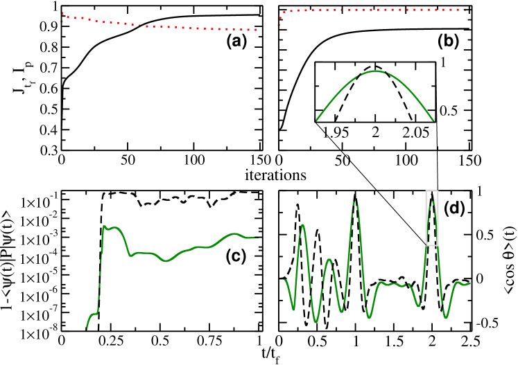
Figure 1: (Color online) Terminal cost $J_{t_{f}}$ (solid black line) and average population of the allowed subspace $I_{p}$ (dashed red line) as a function of the number of iterations for standard optimization (a) and including the state-dependent constraint (b). The corresponding time evolution of the population in the forbidden subspace, $1-\langle\psi(t)|\hat{P}|\psi(t)\rangle$, is shown in panel (c), with (solid green line) and without (dashed black line) state-dependent constraint. The time evolution of the figure of merit for orientation, the expectation value of $\cos\theta$, is displayed in panel (d) for fields optimized with (solid green line) and without (dashed black line) the state-dependent constraint. The parameters $\lambda$ and $\mu$ used in the simulations are fixed to 20 and 50/$t_{f}$, respectively. The small insert in panel (b) represents a zoom of the dynamical evolution near a maximum of $\langle\cos\theta\rangle$.

Figure 1 compares the results obtained by a standard optimization procedure and by one employing the state-dependent constraint. The fidelities achieved by the optimized fields are about 95$\%$ and 91$\%$ for the standard and state-dependent constraint optimization algorithms, respectively. The optimized field without the constraint leads to a larger orientation due to population of states $j>j_{opt}$. This is evident from inspection of the dashed black curve in Fig. 1(c) and corresponds to exploring solutions in the forbidden subspace. At the end of the optimization process, more than 25$\%$ of the population remains in the forbidden subspace. The solid green curve of Fig. 1(c) demonstrates that population stays almost completely within the allowed subspace if the state constraint is taken into account. The population transfer towards the forbidden subspace is reduced by two orders of magnitude. Figure 1(d) shows the time evolution of $\langle\cos\theta\rangle$ during two and a half rotational periods. During the first rotational period the field is on, afterwards the evolution is field-free. The optimized field without the state-dependent constraint achieves a higher molecular orientation than the one obtained with the constraint also in the field-free case, due to the rotational wavepacket being made up of states with high $j$. However, as could be expected, the constraint formulation leads to a longer duration of the orientation in field-free conditions. More precisely, we get a FWHM of 0.086 and 0.136 without and with constraint. The duration of the field-free orientation amounts to what can be expected for a rotational wavepacket being comprised of $j\leq\j_{opt}$ [47].

4.2 Time-optimization of molecular rotation

This section focuses on the production of molecular orientation by a joint optimization of the control time and of the laser fluence. Instead of optimizing the expectation value $|\langle\cos\theta\rangle|$ itself, we choose here a target state $|\phi_{f}\rangle$ which maximizes $|\langle\cos\theta\rangle|$ in a finite-dimensional Hilbert space, $\mathcal{H}_{j_{opt}}$, spanned by the states $\{|j,0\rangle\}$ with $0\leq j\leq j_{opt}$. The details of the construction of $|\phi_{f}\rangle$ are found in Refs. [40, 41]. In the numerical computations, the parameter $j_{opt}$ is fixed to the value 4. The control scheme is the one described in Sec. 2.3 with the guess field of Sec. 4.1.

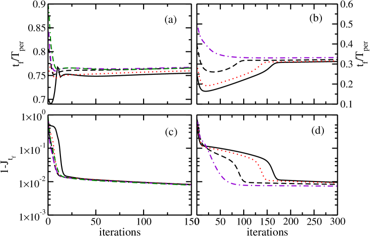
Figure 2: (Color online) Normalized control time $t_{f}/T_{\mathrm{per}}$ as a function of the number of iterations for different values of $t_{f}^{(0)}$ (panels (a) and (b)). Deviation from unity of the corresponding terminal cost (panels (c) and (d)). The parameters $\lambda$ and $\epsilon$ are fixed to 5 and 1000 respectively.

Figure 2(a) and (b) illustrates that $t_{f}$ is indeed independent of the initial time $t_{f}^{(0)}$, a crucial property of the algorithm. Two limit points of the sequence $(t_{f}^{(k)})$ are found for $t_{f}^{0}/T_{\mathrm{per}}\in[0.25,0.9]$. The two attraction points are $t_{f}/T_{\mathrm{per}}\approx 0.31$ for $t_{f}^{(0)}/T_{\mathrm{per}}\in[0.25,0.6]$ and $t_{f}/T_{\mathrm{per}}\approx 0.77$ for $t_{f}^{(0)}/T_{\mathrm{per}}\in[0.75,0.9]$. Note that other limit points can be found if $t_{f}^{(0)}>T_{\mathrm{per}}$. Extensive numerical tests show that the two attraction points are not changed by small modifications of $\lambda$ and the maximum amplitude of the guess field. The optimal solutions corresponding to the two limit points, shown in Fig. 2(c) and (d), have a very similar efficiency.

The numerical algorithm has revealed that two times, clearly shorter than one rotational period, are well-suited to maximize molecular orientation. This result is interesting in view of practical applications since, in standard experimental conditions [42, 43], collisions play a significant role only for times larger than 3 or 4 rotational periods.

5 Conclusion

We have applied two recent formulations of optimal control algorithms to the manipulation of molecular orientation by THz laser fields. Such algorithms have the advantage of simplicity and general applicability for any quantum dynamics. The molecular rotation studied here serves as an illustrative example to demonstrate the efficiency of the methods.

Moreover, our work provides insight into the different ways to produce molecular orientation. For this complicated control problem, there exists no unique optimal solution. A particular pathway can be selected by adding constraints, either on the control field (here the optimization of the control time) or on the state space (here only a subspace of the total Hilbert space is allowed to be populated by the control field). Generally, constraints could also be designed to account for experimental imperfections or requirements related to a specific material or device. The possibility of including such constraints renders the optimal control theory more useful in view of experimental applications and helps bridge the gap between control theory and control experiments.

6 Acknowledgments

We gratefully acknowledge financial support from the Conseil Régional de Bourgogne and the QUAINT coordination action (EC FET-Open).

References

- [1] Pontryagin, L.S.; Boltyanskii, V.G.; Gamkrelidze, R.V.; et al. The mathematical theory of optimal processes. : , 1962.
- [2] Bryson, A.E.; Ho, Y.C. Applied optimal control. : , 1975.
- [3] Rice, S.A.; Zhao, M. Optical control of molecular dynamics. John Wiley & Sons: New York, 2000.
- [4] Brumer, P.; Shapiro, M. Principles and Applications of the Quantum Control of Molecular Processes. Wiley VCH: Weinheim, 2011.
- [5] Somlói, J.; Kazakovski, V.A.; Tannor, D.J. Chem. Phys. 1993, 172, 85–98.
- [6] Zhu, W.; Botina, J.; Rabitz, H. J. Chem. Phys. 1998, 108 (5), 1953–1963.
- [7] Brif, C.; Chakrabarti, R.; Rabitz, H. New J. Phys. 2010, 12 (7), 075008.
- [8] Skinner, T.E.; Reiss, T.O.; Luy, B.; Khaneja, N.; et al. J. Magn. Reson. 2003, 163 (1), 8 – 15.
- [9] Khaneja, N.; Reiss, T.; Kehlet, C.; Schulte-HerbrĂĽggen, T.; et al. Optimal control of coupled spin dynamics: design of {NMR} pulse sequences by gradient ascent algorithms. J. Magn. Reson. 2005, 172 (2), 296 – 305.
- [10] Goerz, M.H.; Calarco, T.; Koch, C.P. J. Phys. B 2011, 44, 154011.
- [11] Doria, P.; Calarco, T.; Montangero, S. Phys. Rev. Lett. 2011, 106, 190501.
- [12] Werschnik, J.; Gross, E.K.U. J. Phys. B 2007, 40 (18), R175–R211.
- [13] Maday, Y.; Turinici, G. J. Chem. Phys. 2003, 118 (18), 8191–8196.
- [14] Sklarz, S.E.; Tannor, D.J. Phys. Rev. A 2002, 66 (5), 053619.
- [15] Palao, J.P.; Kosloff, R. Phys. Rev. A 2003, 68, 062308.
- [16] Reich, D.M.; Ndong, M.; Koch, C.P. J. Chem. Phys. 2012, 136, 104103.
- [17] Ohtsuki, Y.; Nakagami, K. Phys. Rev. A 2008, 77, 033414.
- [18] Lapert, M.; Tehini, R.; Turinici, G.; et al. Phys. Rev. A 2008, 78, 023408.
- [19] Ndong, M.; Lapert, M.; Koch, C.P.; et al. Phys. Rev. A 2013, 87 (Apr), 043416.
- [20] Palao, J.P.; Kosloff, R.; Koch, C.P. Phys. Rev. A 2008, 77, 063412.
- [21] Werschnik, J.; Gross, E. Journal of Optics B: Quantum and Semiclassical Optics 2005, 7 (10), S300–S312.
- [22] Gollub, C.; Kowalewski, M.; de Vivie-Riedle, R. Phys. Rev. Lett. 2008, 101, 073002.
- [23] Schröder, M.; Brown, A. New J. Phys. 2009, 11, 105031 (13pp).
- [24] Lapert, M.; Tehini, R.; Turinici, G.; et al. Phys. Rev. A 2009, 79, 063411.
- [25] Skinner, T.E.; Gershenzon, N.I. J. Magn. Reson. 2010, 204 (2), 248.
- [26] Lapert, M.; Salomon, J.; Sugny, D. Phys. Rev. A 2012, 85, 033406.
- [27] Zhang, Y.; Lapert, M.; Sugny, D.; Braun, M.; et al. J. Chem. Phys. 2011, 134, 054103.
- [28] Mishima, K.; Yamashita, K. J. Chem. Phys. 2009, 130, 034108.
- [29] Mishima, K.; Yamashita, K. J. Chem. Phys. 2009, 131, 014109.
- [30] Stapelfeldt, H.; Seideman, T. Rev. Mod. Phys. 2003, 75, 543–557.
- [31] Seideman, T.; Hamilton, E. Adv. At. Mol. Opt. Phys. 2005, 52, 289 – 329.
- [32] Friedrich, B.; Herschbach, D. Phys. Rev. Lett. 1995, 74, 4623–4626.
- [33] Leibscher, M.; Averbukh, I.S.; Rabitz, H. Phys. Rev. Lett. 2003, 90, 213001.
- [34] Salomon, J.; Dion, C.M.; Turinici, G. J. Chem. Phys. 2005, 123, 144310.
- [35] Abe, H.; Ohtsuki, Y. Phys. Rev. A 2011, 83, 053410.
- [36] Fleischer, S.; Zhou, Y.; Field, R.W.; et al. Phys. Rev. Lett. 2011, 107, 163603.
- [37] Shu, C.C.; Yuan, K.J.; Hu, W.H.; et al. J. Chem. Phys. 2010, 132, 244311.
- [38] Lapert, M.; Sugny, D. Phys. Rev. A 2012, 85, 063418.
- [39] Shu, C.C.; Henriksen, N.E. Phys. Rev. A 2013, 87, 013408.
- [40] Sugny, D.; Keller, A.; Atabek, O.; Daems, D.; Dion, C.M.; Guérin, S.; et al. Phys. Rev. A 2005, 71, 063402.
- [41] Sugny, D.; Keller, A.; Atabek, O.; Daems, D.; Dion, C.M.; Guérin, S.; et al. Phys. Rev. A 2005, 72, 032704.
- [42] Ramakrishna, S.; Seideman, T. Phys. Rev. Lett. 2005, 95, 113001.
- [43] Vieillard, T.; Chaussard, F.; Sugny, D.; Lavorel, B.; et al. J. Raman Spec. 2008, 39 (6), 694–699.
- [44] Kaiser, A.; May, V. J. Chem. Phys. 2004, 121 (6), 2528–2535.
- [45] Şerban, I.; Werschnik, J.; Gross, E.K.U. Phys. Rev. A 2005, 71, 053810.
- [46] Ndong, M.; Tal-Ezer, H.; Kosloff, R.; et al. J. Chem. Phys. 2009, 130, 124108.
- [47] Sugny, D.; Keller, A.; Atabek, O.; Daems, D.; Guérin, S.; et al. Phys. Rev. A 2004, 69, 043407.