The solution of the scalar wave equation in the exterior of a sphere

Abstract

We derive new, explicit representations for the solution to the scalar wave equation in the exterior of a sphere, subject to either Dirichlet or Robin boundary conditions. Our formula leads to a stable and high-order numerical scheme that permits the evaluation of the solution at an arbitrary target, without the use of a spatial grid and without numerical dispersion error. In the process, we correct some errors in the analytic literature concerning the asymptotic behavior of the logarithmic derivative of the spherical modified Hankel function. We illustrate the performance of the method with several numerical examples.

1 Introduction

In this paper, we consider a simple problem, namely the solution of the scalar wave equation

$$u_{tt}=\Delta u,\quad t>0,$$ (1)

subject to homogeneous initial conditions

$$u(r,\theta,\phi,0)=0,\qquad u_{t}(r,\theta,\phi,0)=0$$ (2)

in the exterior of the unit sphere. Here, $(r,\theta,\phi)$ denote the spherical coordinates of a point in ${\mathbb{R}}^{3}$ with $r>1$. Standard textbooks on mathematical physics (such as [5, 11]) present exact solutions for the time-harmonic cases governed by the Helmholtz equation, but generally fail to discuss the difficulties associated with the fully time-dependent case (1). As we shall see, it is a nontrivial matter to develop closed-form solutions, and a surprisingly subtle matter to develop solutions that can be computed without catastrophic cancellation.

In this paper, we restrict our attention to boundary value problems with Dirichlet or Robin conditions. We consider the Dirichlet problem first, and assume we are given data on the boundary of the unit sphere of the form:

$$u(1,\theta,\phi,t)=f(\theta,\phi,t).$$ (3)

It is natural to begin by expanding both $u$ and $f$ in terms of spherical harmonics.

$$u(r,\theta,\phi,t) =\sum_{n=0}^{\infty}\sum_{m=-n}^{n}u_{nm}(r,t)Y_{nm}(\theta,\phi),$$ (4)

$$f(\theta,\phi,t) =\sum_{n=0}^{\infty}\sum_{m=-n}^{n}f_{nm}(t)Y_{nm}(\theta,\phi),$$

where

$$Y_{n}^{m}(\theta,\phi)=\sqrt{\frac{2n+1}{4\pi}}\sqrt{\frac{(n-|m|)!}{(n+|m|)!}}\,P_{n}^{|m|}(\cos\theta)e^{im\phi}\,,$$ (5)

$P_{n}(x)$ is the standard Legendre polynomial of degree $n$, and the associated Legendre functions $P_{n}^{m}$ are defined by the Rodrigues’ formula

$$P_{n}^{m}(x)=(-1)^{m}(1-x^{2})^{m/2}\frac{d^{m}}{dx^{m}}P_{n}(x).$$

We let $\hat{u}_{nm}(r,s)$ and $\hat{f}_{nm}(s)$ denote the Laplace transforms of $u_{nm}(r,t)$ and $f_{nm}(t)$:

$$\hat{u}_{nm}(r,s)=\int_{0}^{\infty}e^{-st}u_{nm}(r,t)dt,$$ (6)

$$\hat{f}_{nm}(s)=\int_{0}^{\infty}e^{-st}f_{nm}(t)dt.$$ (7)

It is straightforward [1] to see that $\hat{u}_{nm}(r,s)$ satisfies the linear second order ordinary differential equation (ODE)

$$r^{2}\hat{u}_{nm}(r,s)_{rr}+2r\hat{u}_{nm}(r,s)_{r}-[s^{2}r^{2}+n(n+1)]\hat{u}_{nm}(r,s)=0,$$

for which the decaying solution as $r\rightarrow\infty$ is the modified spherical Hankel function $k_{n}(sr)$. It follows that

$$\hat{u}_{nm}(r,s)=c_{nm}(s)k_{n}(sr).$$

Matching boundary data on the unit sphere, we have $c_{nm}(s)=\hat{f}_{nm}(s)/k_{n}(s)$, and

$$\hat{u}_{nm}(r,s)=\frac{k_{n}(sr)}{k_{n}(s)}\hat{f}_{nm}(s).$$ (8)

The remaining difficulty is that we have an explicit solution in the Laplace transform domain, but we seek the solution in the time domain. For this, we write the right hand side of (8) in a form for which the inverse Laplace transform can carried out analytically. First, from [1, 10, 12], we have

$$k_{n}(z)=\frac{p_{n}(z)}{z^{n+1}}e^{-z}=\frac{\prod_{j=1}^{n}(z-\alpha_{n,j})}{z^{n+1}}e^{-z},$$ (9)

where $\alpha_{n,j}$ ($j=1,\cdots,n$) are the simple roots of $k_{n}$ lying on the open left half of the complex plane. Thus,

$$\frac{k_{n}(sr)}{k_{n}(s)} =\frac{1}{r}e^{-s(r-1)}\prod_{j=1}^{n}\frac{s-\frac{1}{r}\alpha_{n,j}}{s-\alpha_{n,j}}$$ (10)

$$=\frac{1}{r}e^{-s(r-1)}\left(1+\sum_{j=1}^{n}\frac{a_{n,j}(r)}{s-\alpha_{n,j}}\right),$$

where the second equality follows from an expansion using partial fractions and the coefficients $a_{n,j}$ are given from the residue theorem by the formula:

$$a_{n,j}(r) =\frac{\prod_{k=1}^{n}(\alpha_{n,j}-\frac{1}{r}\alpha_{n,k})}{\prod_{k=1,k\neq j}^{n}(\alpha_{n,j}-\alpha_{n,k})}$$ (11)

$$=\frac{p_{n}(\alpha_{n,j}r)}{r^{n}p^{\prime}_{n}(\alpha_{n,j})}$$

$$=re^{\alpha_{n,j}(r-1)}\frac{k_{n}(\alpha_{n,j}r)}{k^{\prime}_{n}(\alpha_{n,j})},\qquad j=1,\cdots,n.$$

Substituting (10) into (8), we obtain

$$\hat{u}_{nm}(r,s)=\frac{1}{r}\left(1+\sum_{j=1}^{n}\frac{a_{n,j}(r)}{s-\alpha_{n,j}}\right)(e^{-s(r-1)}\hat{f}_{nm}(s)).$$ (12)

Taking the inverse Laplace transform of both sides, we have

$$u_{nm}(r,t)=\frac{1}{r}\left(f_{nm}(t-r+1)+\sum_{j=1}^{n}a_{n,j}(r)\int_{0}^{t-r+1}e^{\alpha_{n,j}(t-r+1-\tau)}f_{nm}(\tau)d\tau\right).$$ (13)

This involves the use of the convolution theorem and the formulas $\mathcal{L}^{-1}\left(\frac{1}{s-\alpha}\right)=e^{\alpha t}$ and $\mathcal{L}^{-1}\left(e^{-s(r-1)}\hat{f}_{nm}(s)\right)=f_{nm}(t-r+1)H(t-r+1)$, where $H$ is the Heaviside function.

Remark 1.

Wilcox [17] studied the solution of the scalar wave equation and derived formula (13) in 1959. In that short note, Wilcox stated that the coefficients $a_{n,j}$ given by (11) grew slowly based on the claim that $\frac{k_{n}(\alpha_{n,j})}{k_{n}^{\prime}(\alpha_{n,j})}=O(n^{1/2})$ as $n\rightarrow\infty$. Unfortunately, this estimate is incorrect. In fact, even after multiplication by the exponentially decaying factor $e^{\alpha_{n,j}(r-1)}$, the coefficients $a_{n,j}$ ($j=1,\cdots,n$) grow exponentially fast as $n\rightarrow\infty$. In the next section, we explain this growth in detail. As a result, even though (13) is very convenient for the purpose of theoretical studies, it cannot be used for numerical calculation due to catastrophe cancellation in carrying out the summation.

Remark 2.

Benedict, Field and Lau [3] have recently developed algorithms for compressing the kernel, which they call the teleportation kernel, arising in sphere-to-sphere propagation of data both for the standard wave equation as well as wave equations arising in linearized gravitational theories. For the wave equation their compressed kernels can be used to perform the same function as our solution of the Dirichlet problem. The largest value of $n$ considered in [3] is $64$. It is as yet unclear if useful compressions for much larger values of $n$ can be constructed using their methods.

1.1 Asymptotic growth of the logarithmic derivative of the spherical modified Bessel function

We first show that the coefficients $a_{n,j}$ ($j=1,\cdots,n$) defined in (11) grow exponentially as $n\rightarrow\infty$, for fixed large $r$. Indeed, Lemma 3 in Section 3 shows that the zeros $\alpha_{n,j}$ of $k_{n}$ satisfy the estimates: $|\alpha_{n,j}|\sim O(n)$ for all $j$ and $|\alpha_{n,j}-\alpha_{n,k}|\propto|j-k|$. Thus when $r$ is large, we have

$$\max_{j}|a_{n,j}(r)| =\max_{j}\left|\frac{\prod_{k=1}^{n}(\alpha_{n,j}-\frac{1}{r}\alpha_{n,k})}{\prod_{k=1,k\neq j}^{n}(\alpha_{n,j}-\alpha_{n,k})}\right|$$ (14)

$$\sim\frac{n^{n}}{n!}$$

$$\sim e^{n},$$

where the last line follows from Stirling’s formula $n!\sim\sqrt{2\pi n}\left(\frac{n}{e}\right)^{n}$. We have computed $\max_{j}|a_{n,j}|$ for $n=1,\cdots,200$ using (11), and plotted them in Figure 1 for $r=2$, clearly exhibiting the exponential growth of $\max_{j}|a_{n,j}|$. We also plot $|a_{n,j}(r)|$ as a function of $j$ for a fixed value of $n$ in Fig. 2.

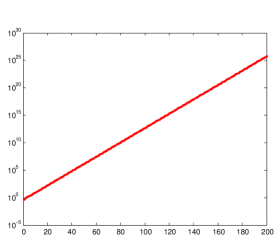
Figure 1: The function $\max_{j}|a_{n,j}(r)|$ for increasing values of $n$, with $r=2$.

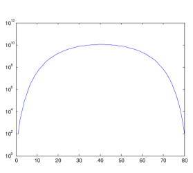
Figure 2: A plot of $|a_{n,j}(r)|$ as a function of $j$, for $n=80$ and $r=2$.

From the preceding analysis, it is clear that one cannot use (13) as stated, since the desired solution is $O(1)$ and catastrophic cancellation will occur in computing $u(r,\theta,\phi,t)$ from exponentially large intermediate quantities.

Fortunately, even though $\max_{j}|a_{n,j}(r)|$ grows exponentially as $n$ increases, we can rewrite (13) in the form of a convolution, which involves much more benign growth:

$$u_{nm}(r,t)=\frac{1}{r}\left(f_{nm}(t-r+1)+\int_{0}^{t-r+1}C_{n}(r,t-r+1-\tau)f_{nm}(\tau)d\tau\right),$$ (15)

where the convolution kernel $C_{n}$ is defined by the formula

$$C_{n}(r,t)=\sum_{j=1}^{n}a_{n,j}(r)e^{\alpha_{n,j}t}.$$ (16)

If we write

$$C_{n}(r,t)=\mathcal{L}^{-1}\left(\hat{C}_{n}(r,s)\right),$$ (17)

then from (11), we have

$$\hat{C}_{n}(r,s) =\prod_{j=1}^{n}\frac{s-\frac{1}{r}\alpha_{n,j}}{s-\alpha_{n,j}}-1=\sum_{j=1}^{n}\frac{a_{n,j}(r)}{s-\alpha_{n,j}}$$ (18)

$$=re^{s(r-1)}\frac{k_{n}(sr)}{k_{n}(s)}-1$$

$$=\sqrt{r}e^{s(r-1)}\frac{K_{n+1/2}(sr)}{K_{n+1/2}(s)}-1,$$

where $K_{n+1/2}$ is the modified Bessel function of the second kind. The last expression follows from the fact that $k_{n}(z)=\sqrt{\frac{2}{\pi z}}K_{n+\frac{1}{2}}(z)$.

The convolution kernel $C_{n}(r,t)$ and its Laplace transform $\hat{C}_{n}(r,s)$ are plotted in Figs. 3 and 4, respectively.

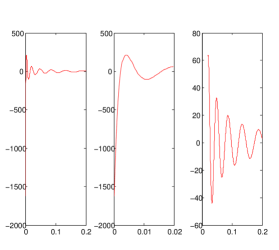
Figure 3: The convolution kernel $C_{n}(r,t)$ as a function of $t$ for $n=80$ and $r=2$. The left-hand plot shows $C_{n}(r,t)$ for $t\in[0,0.2]$, the middle plot shows the same function on $[0,0.02]$, and the right-hand plot shows the function on $[0.02,0.2]$.

Figure 4: The Laplace transform $\hat{C}_{n}(r,s)$ of the convolution kernel is plotted on the imaginary axis over the range $[-1000i,1000i]$ for $n=80$ and $r=2$. The red (lower) curve corresponds to the real part of $\hat{C}_{n}(r,s)$ and the blue (upper) curve corresponds to its imaginary part.

The following lemma shows that the convolution kernel grows only quadratically as a function of $n$ at $t=0$. Numerical experiments (see Fig. 3) suggest that $C_{n}(r,t)$ is maximal in magnitude at $t=0$. Thus, while the sum of exponential expression (16) involves catastrophic cancellation, the function $C_{n}(r,t)$ is, itself, well-behaved and we may seek an alternative method for the evaluation of the convolution integral.

Lemma 1.

Let $r>1$. Then

$$C_{n}(r,0)=\sum_{j=1}^{n}a_{n,j}(r)=\frac{n(n+1)}{2}\left(\frac{1}{r}-1\right).$$ (19)

Proof.

By the initial value theorem for the Laplace transform,

$$C_{n}(r,0)=\lim_{s\rightarrow\infty}s\hat{C}_{n}(r,s).$$ (20)

The first equality in (19) follows from (18). From [1] (formula 9.7.2 on page 378), we have the asymptotic expansion

$$K_{\nu}(z)\sim\sqrt{\frac{\pi}{2z}}e^{-z}\left\{1+\frac{\mu-1}{8z}+\frac{(\mu-1)(\mu-9)}{2!(8z)^{2}}+\cdots\right\},$$ (21)

where $\mu=4\nu^{2}$. Substituting (18) and (21) into (20), we obtain

$$C_{n}(r,0)=\lim_{s\rightarrow\infty}s\left(\frac{1+\frac{\mu-1}{8sr}+O(s^{-2})}{1+\frac{\mu-1}{8s}+O(s^{-2})}-1\right)=\frac{\mu-1}{8}\left(\frac{1}{r}-1\right).$$ (22)

The result (19) now follows from the fact that $\mu=4\nu^{2}=4\left(n+\frac{1}{2}\right)^{2}$. ∎

Despite the fact that $\max_{j}|a_{n,j}(r)|$ grows exponentially with $n$, (19) shows that the sum of weights $a_{n,j}$ is only $O(n^{2})$ for fixed $r$. Still, however, the formula (13) cannot be used in practice because of catastrophic cancellation in the summation

$$\sum_{j=1}^{n}a_{n,j}(r)\int_{0}^{t-r+1}e^{\alpha_{n,j}(t-r+1-\tau)}f_{nm}(\tau)d\tau.$$

Thus, we will need a different representation for the convolution operator $\int_{0}^{t-r+1}C_{n}(r,t-r+1-\tau)f_{nm}(\tau)d\tau$ which is suitable for numerical computation.

1.2 Stable computation of the convolution integral

To obtain a stable formula, we note first that we may rewrite (13) in the form:

$$u_{nm}(r,t)=\frac{1}{r}\int_{0}^{t-r+1}\mathcal{L}^{-1}\left(\hat{C}_{n}(r,s)+1\right)(r,t-r+1-\tau)f_{nm}(\tau)d\tau.$$ (23)

We then use (18) to express $\hat{C}_{n}$ as

$$\hat{C}_{n}(r,s)+1 =\prod_{j=1}^{n}\frac{s-\frac{1}{r}\alpha_{n,j}}{s-\alpha_{n,j}} =\prod_{j=1}^{n}\left(1+\frac{(1-\frac{1}{r})\alpha_{n,j}}{s-\alpha_{n,j}}\right).$$ (24)

We can, therefore, compute $u_{nm}$ recursively:

$$\phi_{0}(t) =f_{nm}(t),$$ (25)

$$\phi_{j}(t) =\phi_{j-1}(t)+\left(1-\frac{1}{r}\right)\alpha_{n,j}\int_{0}^{t}e^{\alpha_{n,j}(t-\tau)}\phi_{j-1}(\tau)d\tau,\quad j=1,\cdots,n$$

and, finally,

$$u_{nm}(r,t)=\frac{1}{r}\phi_{n}(t-r+1).$$ (26)

Numerical experiments indicate that the above recursion is stable if the zeros $\alpha_{n,j}$ of $k_{n}$ are arranged in ascending order according to their real parts, i.e., $\alpha_{n,1}$ is closest to the negative real axis and $\alpha_{n,n}$ is closest to the imaginary axis.

Remark 3.

Alternatively, it is easy to show that the functions $\phi_{j}$ ($j=1,\cdots,n$) are the solutions to the following first order system of ordinary differential equations (ODEs) with zero initial conditions.

$$A\frac{d\phi}{dt}=B\phi+F(t),$$ (27)

where $\phi$ is a column vector of length $n$ with the $j$th entry being $\phi_{j}$, $A$, $B$ are $n\times n$ constant matrices defined by the formulas

$$A=\left(\begin{array}[]{cccc}1&&&0\\ -1&\ddots&&\\ &\ddots&\ddots&\\ 0&&-1&1\end{array}\right),\qquad B=\left(\begin{array}[]{cccc}\alpha_{n,1}&&&0\\ -\frac{\alpha_{n,2}}{r}&\ddots&&\\ &\ddots&\ddots&\\ 0&&-\frac{\alpha_{n,n}}{r}&\alpha_{n,n}\end{array}\right),$$ (28)

and $F$ is a column vector of length $n$ whose only nonzero entry is $F_{1}(t)=f^{\prime}_{nm}(t)-\frac{\alpha_{n,1}}{r}f_{nm}(t)$.

Remark 4.

The ODE system (27) can actually be solved analytically. That is, one may multiply both sides of (27) by $A^{-1}$ to obtain

$$\frac{d\phi}{dt}=M\phi+A^{-1}F(t),$$ (29)

where $M=A^{-1}B$. It is clear that $M$ is a constant lower triangular matrix. One could then diagonalize the system using the eigen-decomposition $M=S\Lambda S^{-1}$. This, however, is numerically unstable since $M$ is a highly nonnormal matrix. Thus, even though the condition number of $M$ is not very high (numerical evidence shows that $\text{cond}(M)=O(n)$), $S$ is extremely ill-conditioned. In fact, more detailed analysis shows that this approach leads exactly to the formula (13). Nevertherless, the ODE system (27) itself can be solved numerically using standard ODE packages, albeit less efficiently than the explicit recursive approach we present in section 3, especially for high precision.

2 The Robin problem

In this section, we consider the Robin problem for the scalar wave equation on the unit sphere:

$$v_{tt}-\Delta v=0,\qquad r>1,\quad t>0,$$ (30)

with homogeneous initial data

$$v(r,\theta,\phi,0)=0,\qquad v_{t}(r,\theta,\phi,0)=0,\qquad r>1,$$ (31)

and the boundary condition

$$\left(\frac{\partial}{\partial r}+1\right)v(r,\theta,\phi,t)=g(\theta,\phi,t),\qquad r=1.$$ (32)

It should be noted that Tokita [14] extended Wilcox’s analysis of the Dirichlet problem to the case of Robin boundary conditions of the form $(\frac{\partial}{\partial r}+\sigma)v=g$, although he assumed that $\sigma<1$ in his discussion. We are primarily concerned with the case $\sigma=1$ since it arises in the solution of the full Maxwell equations [7].

As in the analysis of the Dirichlet problem, we first expand $v$ and $g$ in terms of spherical harmonics, perform the Laplace transform in $t$, match the boundary data and obtain

$$v(r,\theta,\phi,t) =\sum_{n=0}^{\infty}\sum_{m=-n}^{n}\mathcal{L}^{-1}(\hat{v}_{nm}(r,s))Y_{nm}(\theta,\phi),$$ (33)

$$g(\theta,\phi,t) =\sum_{n=0}^{\infty}\sum_{m=-n}^{n}\mathcal{L}^{-1}(\hat{g}_{nm}(s))Y_{nm}(\theta,\phi),$$

and

$$\hat{v}_{nm}(r,s)=\frac{k_{n}(sr)}{sk^{\prime}_{n}(s)+k_{n}(s)}\hat{g}_{nm}(s).$$ (34)

We turn now to a study the properties of the kernel in (34), letting

$$\mathcal{K}_{n}(r,s)=\frac{k_{n}(sr)}{sk^{\prime}_{n}(s)+k_{n}(s)},$$ (35)

and

$$D_{n}(z)=zk^{\prime}_{n}(z)+k_{n}(z).$$ (36)

Recalling from 9 that $k_{n}(z)=\frac{p_{n}(z)}{z^{n+1}}e^{-z}$, we have

$$D_{n}(z)=\frac{-zp_{n}(z)-np_{n}(z)+zp^{\prime}_{n}(z)}{z^{n+1}}e^{-z}\equiv\frac{q_{n+1}(z)}{z^{n+1}}e^{-z}.$$ (37)

Hence,

$$\mathcal{K}_{n}(r,s)=\frac{1}{r}\frac{p_{n}(sr)}{q_{n+1}(s)r^{n}}e^{-s(r-1)}.$$ (38)

In particular, for $n=0$, we have

$$\mathcal{K}_{0}(r,s)=-\frac{1}{rs}e^{-s(r-1)}.$$ (39)

Obviously, the poles of $\mathcal{K}_{n}$ are simply the zeros of $D_{n}$. Those zeros have been characterized by Tokita [14] in the following lemma.

Lemma 2.

[adapted from [14].] For $n\geq 1$, $D_{n}(z)=zk^{\prime}_{n}(z)+k_{n}(z)$ has $n+1$ simple roots denoted by $\{\beta_{n,0},\cdots,\beta_{n,n}\}$. All the roots lie in the open left half of the complex plane symmetrically with respect to the real axis. Furthermore, they satisfy the following estimates

$$\Re\beta_{n,j}<-An^{\frac{1}{3}},$$ (40)

$$|\beta_{n,j}|<Bn,$$ (41)

for sufficiently large $n$ and $0\leq j\leq n$. Hence, there exists a positive number $\mu$ such that

$$\Re\beta_{n,j}<-\mu,$$ (42)

for all $n\geq 1$ and $0\leq j\leq n$.

From the preceding lemma, for $n\geq 1$ we have

$$\mathcal{K}_{n}(r,s) =\frac{1}{r}e^{-s(r-1)}\frac{\prod_{j=1}^{n}\left(s-\frac{1}{r}\alpha_{n,j}\right)}{-\prod_{j=0}^{n}(s-\beta_{n,j})}$$ (43)

$$=-\frac{1}{r}e^{-s(r-1)}\frac{1}{s-\beta_{n,0}}\prod_{j=1}^{n}\left(1+\left(\beta_{n,j}-\frac{1}{r}\alpha_{n,j}\right)\frac{1}{s-\beta_{n,j}}\right).$$

One could carry out a partial fraction expansion for the right hand side of (43) to obtain

$$\mathcal{K}_{n}(r,s)=\frac{1}{r}e^{-s(r-1)}\sum_{j=0}^{n}\frac{b_{n,j}(r)}{s-\beta_{n,j}},$$ (44)

where the coefficients $b_{n,j}$ are given by the formula

$$b_{n,j}(r) =-\frac{\prod_{k=1}^{n}\left(\beta_{n,j}-\frac{1}{r}\alpha_{n,k}\right)}{\prod_{k=0,k\neq j}^{n}(\beta_{n,j}-\beta_{n,k})}$$ (45)

$$=\frac{p_{n}(\beta_{n,j}r)}{r^{n}q^{\prime}_{n+1}(\beta_{n,j})}$$

$$=re^{\beta_{n,j}(r-1)}\frac{k_{n}(\beta_{n,j}r)}{D^{\prime}_{n}(\beta_{n,j})}.$$

This would yield

$$v_{nm}=\frac{1}{r}\sum_{j=0}^{n}b_{n,j}(r)\int_{0}^{t-r+1}e^{\beta_{n,j}(t-r+1-\tau)}g_{nm}(\tau)d\tau,\qquad n>0.$$ (46)

Unfortunately, the coefficients $b_{n,j}$ ($j=0,\cdots,n$) behave as badly as the coefficients $a_{n,j}$ defined in (11) for the Dirichlet problem. That is, catastrophic cancellation in (46) makes it ill-suited for numerical computation.

Fortunately, as in section 1.2, we can compute $v_{nm}$ without catastrophic cancellation using the following recurrence ($\beta_{0,0}=0$):

$$\psi_{0}(t) =\int_{0}^{t}e^{\beta_{n,0}(t-\tau)}g_{nm}(\tau)d\tau,$$ (47)

$$\psi_{j}(t) =\psi_{j-1}(t)+\left(\beta_{n,j}-\frac{1}{r}\alpha_{n,j}\right)\int_{0}^{t}e^{\beta_{n,j}(t-\tau)}\psi_{j-1}(\tau)d\tau,\quad j=1,\cdots,n,$$

with

$$v_{nm}(r,t)=-\frac{1}{r}\psi_{n}(t-r+1).$$ (48)

We leave the derivation of the recurrence to the reader.

Remark 5.

It is possible to write down a system of ODEs that is equivalent to (47). We omit details since the derivation is straightforward and we prefer the recurrence for numerical purposes in any case.

3 A numerical method

In order to carry out the recurrences (25) or (47), we first need to compute to compute the zeros of $k_{n}(z)$ and $D_{n}(z)$. The following lemma provides asymptotic approximations of the zeros of these two functions, which we will use as initial guesses followed by a simple Newton iteration. In practice, we have found that six Newton steps are sufficient to achieve double precision accuracy for $n<10,000$.

Lemma 3.

(Asymptotic distribution of the zeros of $k_{n}(z)$ and $D_{n}(z)$, adapted from [10, 14]); see also the appendix.

1. The zeros of $k_{n}(z)$ have the following asymptotic expansion

   $$\alpha_{n,j}\sim n(z(\zeta_{j})+O(n^{-1})),\text{ $n\rightarrow\infty$},$$ (49)

   uniformly in $j$, where $\zeta_{j}$ is defined by the formula

   $$\zeta_{j}=e^{-2\pi i/3}\left(n+\frac{1}{2}\right)^{-2/3}a_{j},$$ (50)

   $a_{j}$ is the $j$th negative zero of the Airy function $Ai$ whose asymptotic expansion is given by the formula

   $$a_{j}\sim-(\frac{3\pi}{2})^{2/3}(j-\frac{1}{4})^{2/3}+O(j^{-4/3}),$$ (51)

   and $z(\zeta)$ is obtained from inverting the equation

   $$\frac{2}{3}\zeta^{3/2}=\ln{\frac{i(1+\sqrt{1+z^{2}})}{z}}-\sqrt{1+z^{2}},$$ (52)

   where the branch is chosen so that $\zeta$ is real when $z$ is positive imaginary. In other words, $z(\zeta)$ lies on the curve whose parametric equation is

   $$z(t)=-(t^{2}-t\tanh{t})^{1/2}\pm i(t\coth{t}-t^{2})^{1/2},$$ (53)

   where $t\in[0,t_{0}]$ and $t_{0}=1.19968\ldots$ is the positive root of $t=\coth{t}$.

2. The zeros of $D_{n}(z)=zk^{\prime}_{n}(z)+k_{n}(z)$ have the asymptotic expansion

   $$\beta_{n,j}\sim n(z(\xi_{j})+O(n^{-1})),\text{ $n\rightarrow\infty$},$$ (54)

   uniformly in $j$, where $\xi_{j}$ is defined by the formula

   $$\xi_{j}=e^{-2\pi i/3}\left(n+\frac{1}{2}\right)^{-2/3}b_{j},$$ (55)

   and $b_{j}$ is the $j$th negative zero of the first derivative of the Airy function $Ai^{\prime}$ whose asymptotic expansion is given by the formula

   $$b_{j}\sim-(\frac{3\pi}{2})^{2/3}(j-\frac{3}{4})^{2/3}+O(j^{-4/3}),$$ (56)

   and $z(\xi)$ is defined as in (52) with $\zeta$ replaced by $\xi$.

Figure 5 shows the zeros of $k_{10}(z)$, $D_{10}(z)$, $k_{11}(z)$ and $D_{11}(z)$.

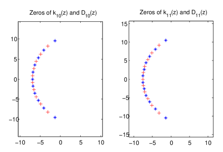
Figure 5: Zeros of $k_{10}(z)$, $D_{10}(z)$, $k_{11}(z)$ and $D_{11}(z)$. The zeros of $k_{n}$ are marked by red $+$, and the zeros of $D_{n}$ are marked by blue $\ast$.

3.1 Marching in time

We now present a high-order discretization scheme for computing $u_{nm}$ and $v_{nm}$. We will only discuss the computation of $u_{nm}$ in detail, since the treatment of $v_{nm}$ is analogous. Recall that the relevant recurrence relations are (25) and (26). To proceed, we first introduce the auxillary functions

$$h_{j}(t)=\int_{0}^{t}e^{\alpha_{n,j}(t-\tau)}\phi_{j-1}(\tau)d\tau,\qquad j=1,\cdots,n.$$ (57)

Then, (25) becomes

$$\phi_{j}(t)=\phi_{j-1}(t)+\left(1-\frac{1}{r}\right)\alpha_{n,j}h_{j}(t).$$ (58)

It is easy to check that $h_{j}(k\Delta t)$ satisfies the recurrence relation

$$h_{j}(k\Delta t)=e^{\alpha_{n,j}\Delta t}h_{j}((k-1)\Delta t)+\int_{(k-1)\Delta t}^{k\Delta t}e^{\alpha_{n,j}(k\Delta t-\tau)}\phi_{j-1}(\tau)d\tau.$$ (59)

Thus, we need only consider the calculation of the integral over $[(k-1)\Delta t,k\Delta t]$. For this, we interpolate $\phi_{j-1}(\tau)$ by a polynomial of degree $p-1$ with the shifted and scaled Legendre nodes as interpolation nodes. That is,

$$\phi_{j-1}(\tau) \approx\sum_{i=0}^{p-1}c_{i}P_{i}\left(\frac{2}{\Delta t}(\tau-(k-\frac{1}{2})\Delta t)\right)$$ (60)

$$=\sum_{i=0}^{p-1}\sum_{l=1}^{p}u_{il}\phi_{j-1}((k-1)\Delta t+\Delta t(1+x_{l})/2)P_{i}\left(\frac{2}{\Delta t}(\tau-(k-\frac{1}{2})\Delta t)\right),$$

where $x_{l}$ ($l=1,\cdots,p$) are the standard Legendre nodes on $[-1,1]$ and $u_{il}$ is the $(i,l)$ entry of the matrix converting function values to the coefficients of a Legendre expansion.

Substituting (60) into the integral on the right side of (59) and simplifying, we obtain

$$\int_{(k-1)\Delta t}^{k\Delta t}e^{\alpha(k\Delta t-\tau)}\phi_{j-1}(\tau)d\tau$$ (61)

$$\approx\sum_{l=1}^{p}u_{il}\phi_{j-1}((k-1)\Delta t+\Delta t(1+x_{l})/2)$$

$$\cdot\frac{\Delta t}{2}\sum_{i=0}^{p-1}\int_{-1}^{1}e^{\alpha_{n,j}\frac{\Delta t}{2}(1-y)}P_{i}(y)dy$$

$$=\sum_{l=1}^{p}q_{l}(\alpha_{n,j})\phi_{j-1}((k-1)\Delta t+\Delta t(1+x_{l})/2),$$

where the coefficients $q_{l}$ ($l=1,\cdots,p$) are given by the formula

$$q_{l}(\alpha_{n,j})=\frac{\Delta t}{2}\sum_{i=0}^{p-1}u_{il}\int_{-1}^{1}e^{\alpha_{n,j}\frac{\Delta t}{2}(1-y)}P_{i}(y)dy.$$ (62)

Substituting (61) into (59), we obtain

$$h_{j}(k\Delta t)=e^{\alpha_{n,j}\Delta t}h_{j}((k-1)\Delta t)+\sum_{l=1}^{p}q_{l}(\alpha_{n,j})\phi_{j-1}((k-1)\Delta t+\Delta t(1+x_{l})/2).$$ (63)

In order to be able to use (63), we need to calculate $\phi_{j-1}((k-1)\Delta t+\Delta t/2(1+x_{l}))$. For this, we can again apply the recurrence (25) and obtain

$$\phi_{0}((k-1)\Delta t+\Delta t(1+x_{l})/2)=f_{nm}((k-1)\Delta t+\Delta t/2(1+x_{l})),$$ (64)

$$\phi_{j}((k-1)\Delta t+\Delta t(1+x_{l})/2)=\phi_{j-1}((k-1)\Delta t+\Delta t/2(1+x_{l}))$$

$$+\left(1-\frac{1}{r}\right)\alpha_{n,j}e^{\alpha_{n,j}\Delta t(1+x_{l})/2}h_{j}((k-1)\Delta t)$$

$$+\left(1-\frac{1}{r}\right)\alpha_{n,j}\sum_{s=1}^{p}w_{ls}(\alpha_{n,j})\phi_{j-1}((k-1)\Delta t+\Delta t/2(1+x_{s})),$$

where the coefficients $w_{ls}$, for $l,s\in\{1,\dots,p\}$, are given by the formula

$$w_{ls}(\alpha_{n,j})=\frac{\Delta t}{2}\sum_{i=0}^{p-1}u_{is}\int_{-1}^{x_{l}}e^{\alpha_{n,j}\frac{\Delta t}{2}(x_{l}-y)}P_{i}(y)dy.$$ (65)

In summary, the algorithm for computing $u_{nm}(r,T)$ proceeds in two stages: a precomputation stage and a time-marching stage.

Algorithm 1 Precomputation phase

0:  For spherical harmonic order $n$, time step $\Delta t$, and desired order of accuracy $p$, precompute the coefficients needed in the marching scheme for $u_{nm}$.

1:  Compute and store the zeros $\alpha_{n,j}$ ($j=1,\cdots,n$) of $k_{n}$.

2:  Compute the Legendre nodes $x_{l}$ ($l=1,\cdots,p$) and the $p\times p$ matrix $u$ which converts function values to the coefficients of the corresponding Legendre expansion.

3:  for $j=1:n$ and $i=1:p$ do

4:        Compute the integrals $\int_{-1}^{1}e^{\alpha_{n,j}\frac{\Delta t}{2}(1-y)}P_{i}(y)dy$.

5:  end for

6:  for $j=1:n$ and $i=1:p$ do

7:        Compute and store the coefficients $q_{l}(\alpha_{n,j})$ defined in (62).

8:  end for

9:  for $j=1:n$, $i=1:p$, and $l=1:p$ do

10:        Compute the integrals $\int_{-1}^{x_{l}}e^{\alpha_{n,j}\frac{\Delta t}{2}(x_{l}-y)}P_{i}(y)dy$.

11:  end for

12:  for $j=1:n$, $s=1:p$, and $l=1:p$ do

13:        Compute and store the coefficients $w_{ls}(\alpha_{n,j})$ defined in (65).

14:  end for

15:  for $j=1:p$ do

16:        Compute and store $e^{\alpha_{n,j}\Delta t}$.

17:  end for

18:  for $j=1:n$ and $l=1:p$ do

19:        Compute and store $e^{\alpha_{n,j}\Delta t(1+x_{l})/2}$.

20:  end for

Algorithm 2 Marching in time

0:  Given $n$, $r$, $T$, the desired order of accuracy $p$, and the number of desired time steps $N_{T}$, compute the spherical harmonic mode $u_{nm}$ at $(r,T)$ defined by (26).

1:  Set $\Delta t=(T-r+1)/N_{T}$.

2:  for $j=1:n$ do

3:        Set $h_{j}=0$.

4:  end for

5:  for $k=1:N_{T}$ do

6:        for $l=1:p$ do

7:              Evaluate the boundary data $f_{nm}((k-1)\Delta t+\Delta t(1+x_{l})/2)$ by computing the spherical harmonic transform of the Dirichlet data $f$, and set $\phi_{0}((k-1)\Delta t+\Delta t(1+x_{l})/2)=f_{nm}((k-1)\Delta t+\Delta t/2(1+x_{l}))$.

8:        end for

9:        for $j=1:n$ and $l=1:p$ do

10:              Use (64) to compute $\phi_{j}((k-1)\Delta t+\Delta t(1+x_{l})/2)$

11:        end for

12:        for $j=1:n$ do

13:              Use (63) to update $h_{j}$.

14:        end for

15:  end for

16:  Set $u_{nm}=f_{nm}(N_{T}\Delta t)$.

17:  for $j=1:n$ do

18:        Compute $u_{nm}=u_{nm}+\left(1-\frac{1}{r}\right)\alpha_{n,j}h_{j}$.

19:  end for

20:  Compute $u_{nm}=u_{nm}/r$.

3.2 Computational complexity

For each spherical harmonic mode, it is easy to see that the precomputation cost is $O(np^{2})$ and the marching cost is $O(np^{2}N_{T})$, where $p$ is the desired order of accuracy and $N_{T}$ is the total number of time steps. Thus, if we truncate the spherical harmonic expansion order at $N$, then the precomputation cost is $O(N^{2}p^{2})$ and the marching cost is $O(N^{3}p^{2}N_{T})$. The cost of computing the spherical harmonic transform of the boundary data at all times is $O(N^{3}N_{T}p)$ and the cost of the inverse spherical harmonic transform at the final time is $O(N^{3})$. Summing all these factors up, we observe that the total computational cost of our algorithm is $O(N^{3}p^{2}N_{T})$.

4 Numerical examples

We have implemented the above algorithm in Fortran for both the Dirichlet and Robin problems governed by the scalar wave equation. To test its convergence and stability, we consider the exact solution

$$u(x,t)=\sum_{i=1}^{2}c_{i}e^{-(t-t_{i}-|x-y_{i}|)^{2}/a_{i}}\cos(k_{i}(t-|x-y_{i}|))/|x-y_{i}|$$ (66)

with $y_{1}=(0.3,-0.5,0.6)$, $t_{1}=1.2$, $a_{1}=0.05$, $k_{1}=100$, and $y_{2}=(-0.4,-0.5,0.7)$, $t_{2}=3.2$, $a_{2}=0.28$, $k_{2}=80$. The numerical solution is computed on a sphere of radius $r=100$ at $t=103$.

Tables 1-4 show the relative $L^{2}$ error of the numerical solution of the scalar wave equation for varying values of $N$, the order of the spherical expansion and total number of time steps. Note that the solution is oscillatory in both space and time, so that finite difference or finite element methods would have difficulty computing the solution in the far field with high precision because of numerical dispersion errors. In Tables 1 and 3, the order of temporal convolution is $p=10$ and we break the time interval $[99,103]$ into $200$ equispaced subintervals (yielding a total of $2000$ discretization points in time). In Tables 2 and 4, we use $80$ terms in the spherical harmonic expansions. These tables show that numerical solution converges spectrally fast to the exact solution.

$N_{S}$	102400	129600	160000	193600	230400	270400
$N$	80	90	100	110	120	130
$E$	0.84E-01	0.65E-03	0.12E-05	0.64E-09	0.89E-12	0.88E-12

Table 1: Relative $L^{2}$ error of the numerical solution of the Dirichlet problem with increasing spherical harmonic expansion order $N$. $N_{S}$ is the total number of discretization on the unit sphere. Since the discretization error is usually greater than the truncation error, $N_{\theta}=N_{\phi}$ is chosen to be $4N$. Thus $N_{S}=16N^{2}$. The total number of discretization points in time is $N_{T}=2000$.

$N_{T}$	250	500	750	1000	1500	2000
$E$	0.19E+00	0.12E-03	0.15E-05	0.30E-07	0.47E-10	0.88E-12

Table 2: Relative $L^{2}$ error of the numerical solution of the Dirichlet problem as a function of the total number of discretization points in time. Here, the spherical harmonic expansion order was set to $125$ and the total of number of discretization points on the unit sphere is $N_{S}=250000$. The order of integration for temporal convolution is fixed at $p=10$.

$N_{S}$	102400	129600	160000	193600	230400	270400
$N$	80	90	100	110	120	130
$E$	0.84E-01	0.65E-03	0.12E-05	0.64E-09	0.71E-12	0.70E-12

Table 3: Relative $L^{2}$ error of the numerical solution of the Robin problem with increasing spherical harmonic expansion order $N$. $N_{S}$ is the total number of discretization on the unit sphere. Since the discretization error is usually greater than the truncation error, $N_{\theta}=N_{\phi}$ is chosen to be $4N$. Thus $N_{S}=16N^{2}$. The total number of discretization points in time is $N_{T}=2000$.

$N_{T}$	250	500	750	1000	1250	1500
$E$	0.92E-02	0.13E-05	0.41E-07	0.15E-08	0.58E-10	0.33E-11

Table 4: Relative $L^{2}$ error of the numerical solution of the Robin problem as a function of the total number of discretization points in time. Here, the spherical harmonic expansion orer is $125$ and the total of number of discretization points on the unit sphere is $N_{S}=250000$. The order of integration for temporal convolution is $p=10$.

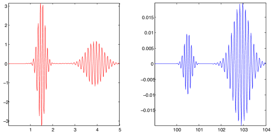
Figure 6: The left-hand plot shows the value of the boundary data at the north pole of the unit sphere as a function of time, and the right-hand plot shows the solution at the north pole of the outer sphere of radius $r=100$. The exact solution is of the same form as (66) - that is, induced by two sources in the interior of the unit sphere.

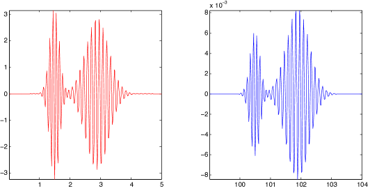
Figure 7: The analog of Fig. 6 for a “true” scattering problem. Dirichlet boundary conditions are generated by two exterior sources placed on the $z$-axis, at $(0,0,1.3)$ and $(0,0,1.7)$. The left-hand plot shows the value of the boundary data at the north pole of the unit sphere as a function of time, and the right-hand plot shows the solution at the north pole of the outer sphere of radius $r=100$.

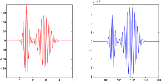
Figure 8: The analog of Fig. 6 for a “true” scattering problem. Robin boundary conditions are generated by two exterior sources placed on the $z$-axis, at $(0,0,1.3)$ and $(0,0,1.7)$. The left-hand plot shows the value of the boundary data at the north pole of the unit sphere as a function of time, and the right-hand plot shows the solution at the north pole of the outer sphere of radius $r=100$.

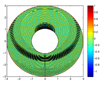
Figure 9: We plot the solution of the field scattered by the unit sphere in the $xz$-plane within the annular region $1<r<3$ at $t=4$. with boundary data as in Fig. 7. Note that the domain is approximately 50 wavelengths in size.

5 Conclusions

We have presented an analytic solution for the scalar wave equation in the exterior of a sphere in a form that is numerically tractable and permits high order accuracy even for objects many wavelengths in size. Aside from its intrinsic interest in single or multiple scattering from a collection of spheres, our algorithm provides a useful reference solution for any numerical method designed to solve problems of exterior scattering. At the present time, such codes are typically tested by Fourier transformation after a long-time simulation and comparison with a set of single frequency solutions computed by separation of variables applied to the Helmholtz equation.

Remark 6.

An exception is the work of Sauter and Veit [13], who make use of a formulation equivalent to that of Wilcox to develop a benchmark solution for a time-domain integral equation solver which can be applied to scattering from general geometries. Exponential ill-conditioning is avoided by considering only low-order spherical harmonic expansions. Recently, Grote and Sim [8] have also used an approach based on the local exact radiation boundary conditions proposed in [9] to develop a new hybrid asymptotic/finite difference formalism for multiple scattering in the time domain. The advantage of the Grote-Sim method is that spherical harmonic transformations are unnecessary and the evaluation formulas can be localized in angle. However, they also restrict their attention to low-order expansions, and our preliminary experiments using their formulas indicate a loss of conditioning for $n$ large. (The loss of conditioning presumably also applies to the radiation boundary conditions in [9].) The method developed here should be of immediate use in both contexts

As implemented above, our algorithm has $O(N^{3}N_{T})$ complexity. It is possible, however, to reduce the cost to $O(N^{2}\log NN_{T})$. This requires the use of a fast spherical harmonic transform (see, for example, [15] and references therein). With this fast algorithm, the cost of each spherical harmonic transform is reduced from $O(N^{3})$ to $O(N^{2}\log N)$. Second, we believe that the convolution kernels can be compressed as in [2], so that they involve only $O(\log n)$ modes for each $n$ for a given precision. We note that compressions for $n=64$ and various radii are reported in [3], both for the scalar wave equation considered here (which they call the flat-space wave equation) and for wave equations with Zerilli and Regge-Wheeler potentials. In the latter cases, compressed kernels are also constructed for smaller values of $n$, as the exact kernels do not have rational transforms. Tabulated coefficients required for implementing the compressed kernels may be found online [18].

For the extension of the present approach to the full Maxwell equations, see [7]. Software implementing the algorithm of the present paper will be made available upon request.

6 Appendix: asymptotic analysis of exponential growth of the coefficients $a_{n,j}$ in (11)

An alternative analysis of the instability phenomenon can be carried out using the uniform asymptotic expansions of the Bessel functons due to Olver [12]. We first recall the relationship between $K_{n+1/2}$ and the Hankel function, $H_{n+1/2}^{(1)}$:

$$K_{n+1/2}(z)=\frac{\pi i}{2}e^{i(n+1/2)\pi}H_{n+1/2}^{(1)}(iz).$$ (67)

Thus the residues we wish to estimate are given by

$$a_{n,j}(r)=\sqrt{r}e^{(r-1)\alpha_{n,j}}\frac{K_{n+1/2}(\alpha_{n,j}r)}{K_{n+1/2}^{\prime}(\alpha_{n,j})}=-i\sqrt{r}e^{(r-1)\alpha_{n,j}}\frac{H_{n+1/2}^{(1)}(i\alpha_{n,j}r)}{H_{n+1/2}^{(1)\ \prime}(i\alpha_{n,j})}.$$ (68)

To approximate these for $n\gg 1$ we use (see [12]):

$$H_{n+1/2}^{(1)}\left(\left(n+\frac{1}{2}\right)w\right)\sim$$ (69)

$$2e^{-\pi i/3}\left(n+\frac{1}{2}\right)^{-1/3}\left(\frac{4\zeta}{1-w^{2}}\right)^{1/4}{\rm Ai}\left(e^{2\pi i/3}\left(n+\frac{1}{2}\right)^{2/3}\zeta\right),$$

$$H_{n+1/2}^{(1)\ \prime}\left(\left(n+\frac{1}{2}\right)w\right)\sim$$ (70)

$$\frac{4e^{-2\pi i/3}}{w}\left(n+\frac{1}{2}\right)^{-2/3}\left(\frac{4\zeta}{1-w^{2}}\right)^{-1/4}{\rm Ai}^{\prime}\left(e^{2\pi i/3}\left(n+\frac{1}{2}\right)^{2/3}\zeta\right),$$

which hold uniformly in $\arrowvert{\rm arg}(w)\arrowvert<\pi-\delta$; thus in particular they hold in $\Re z<0$ where we will be using them. Here $\zeta$ is given by (52) with the replacement $z=iw$.

To proceed we recall the basic properties of the Airy function, ${\rm Ai}(y)$, which are listed in the Appendix of [12] as well as [1, Ch. 10]:

i.

${\rm Ai}(y)$ has infinitely many zeros which lie on the negative real axis. For $j$ large the jth zero, $a_{j}$, of ${\rm Ai}(y)$ satisfies (51) and the derivative satisfies

$${\rm Ai}^{\prime}(a_{j})\sim(-1)^{j-1}\frac{1}{\sqrt{\pi}}\left(\frac{3}{2}\pi j\right)^{1/6}.$$ (71)

ii.

For $\arrowvert{\rm arg}(y)\arrowvert<\pi$ the function ${\rm Ai}(y)$ satisfies the asymptotic formula

$${\rm Ai}(y)\sim\frac{1}{2\sqrt{\pi}}y^{-1/4}e^{-\frac{2}{3}y^{3/2}},\ \ \arrowvert y\arrowvert\gg 1.$$ (72)

Using (i.) we deduce that the poles, $\alpha_{n,j}$, are asymptotically given by (49) and approximately lie on the curve $nz(t)$ where $z(t)$ is defined in (53). This is the curve for which $e^{2\pi i/3}\zeta(z)$ is real and negative.

To evaluate the residues we must calculate using (69),(70)

$$a_{n,j} \sim \sqrt{r}e^{(r-1)\alpha_{n,j}}\alpha_{n,j}\left(n+\frac{1}{2}\right)^{1/3}\left(\frac{\zeta\ \zeta_{r}}{(1+\alpha_{n,j}^{2}r^{2})(1+\alpha_{n,j}^{2})}\right)^{1/4}$$ (73)

$$\times\frac{{\rm Ai}\left(e^{2\pi i/3}\left(n+\frac{1}{2}\right)^{2/3}\zeta_{r}\right)}{{\rm Ai}^{\prime}(a_{j})},$$

where we have introduced

$$\zeta_{r}=\zeta(\alpha_{n,j}r).$$ (74)

Obviously the scaling $z\rightarrow rz$ moves $\zeta_{r}$ off the curve where the argument of the Airy function is real and negative. Thus using (72) and (52) we deduce that the asymptotic formula for $a_{n,j}$ contains an exponential term

$$a_{n,j} \propto e^{(r-1)\alpha_{n,j}-\frac{2}{3}(n+1/2)\zeta_{r}^{3/2}}$$

$$= \exp\left[\left(n+\frac{1}{2}\right)\eta_{n,j}(r)\right]$$

where

$$\eta_{n,j}(r)=\left((r-1)\tilde{\alpha}_{n,j}-\ln\left(\frac{1+\sqrt{1+\tilde{\alpha}_{n,j}^{2}r^{2}}}{i\tilde{\alpha}_{n,j}r}\right)+\sqrt{1+\tilde{\alpha}_{n,j}^{2}r^{2}}\right).$$ (76)

Here we have introduced $\tilde{\alpha}_{n,j}=\left(n+\frac{1}{2}\right)^{-1}\alpha_{n,j}$.

Finally, we consider the real part of the expression in parentheses on the second line of (6). In particular we replace $\tilde{\alpha}_{n,j}$ by a continuous variable $\alpha$ traversing the scaled curve, $z(t)$, containing the approximate zeros. Then the function $\eta$ depends only on $r$ and the coordinate describing the curve; in particular it is independent of $n$ and $j$. In Fig. 10 we plot the real part of $\eta$ scaled by $\log_{10}{e}$ for $r=2$. This can be compared with Fig. 2 by scaling both axes by $n=80$ and recognizing the vertical axis as the base ten logarithm. We then observe good agreement with the numerical results. The maximum value plotted in Figure 10 is approximately $.13$, which is the predicted slope of the straight line plotted in Fig. 1. Again the agreement is good. We note that increasing $r$ makes the problem somewhat worse; the scaled maximum real part is approximately $.23$ for $r=5$ and $.27$ for $r=20$.

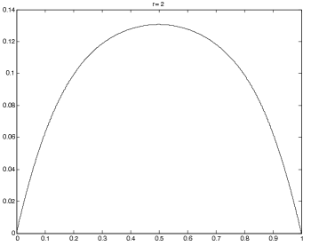
Figure 10: Base 10 exponent of the exponential part of the asymptotic formula for the residue scaled by $n+1/2$.

References

- [1] M. Abramowitz and I. Stegun, Handbook of Mathematical Functions, Dover, New York, 1965.
- [2] B. Alpert, L. Greengard, and T. Hagstrom, Rapid evaluation of nonreflecting boundary kernels for time-domain wave propagation, SIAM J. Numer. Anal. 37 (2000), 1138–1164.
- [3] A. Benedict, S. Field, and S. Lau, Fast evaluation of asymptotic waveforms from gravitational perturbations, Class. Quantum Grav. 30 (2013), 055015.
- [4] E. Carrascal, G. A. Estevez, P. Lee, and V. Lorenzo, Vector spherical harmonics and their application to classical electrodynamics, Eur. J. Phys. 12 (1991), 184-191.
- [5] R. Courant and D. Hilbert (1953), Methods of Mathematical Physics, Interscience Publishers, New York.
- [6] C. Epstein and L. Greengard, Debye Sources and the Numerical Solution of the Time Harmonic Maxwell Equations, Comm. Pure Appl. Math. 63 (2010), 413–463.
- [7] L. Greengard, T. Hagstrom, and S. Jiang, Extension of the Debye-Mie-Lorenz formalism to the time domain in preparation.
- [8] M. Grote and I. Sim, Local nonreflecting boundary condition for time-dependent multiple scattering, J. Comput. Phys. 230 (2011), 3135–3154.
- [9] T. Hagstrom and S. Hariharan, A formulation of asymptotic and exact boundary conditions using local operators, Appl. Numer. Math. 27 (1998), 403–416.
- [10] S. Jiang, Fast Evaluation of the Nonreflecting Boundary Conditions for the Schrödinger Equation, Ph.D. thesis, Courant Institute of Mathematical Sciences, New York University, New York, 2001.
- [11] P. Morse and H. Feshbach (1953), Methods of Theoretical Physics, McGraw-Hill, New York.
- [12] F. W. Olver, The asymptotic expansion of Bessel functions of large order, Philo. Trans. Roy. Soc. London A247 (1954), 328-368.
- [13] S. Sauter and A. Veit, A Galerkin method for retarded boundary integral equations with smooth and compactly supported temporal basis functions Numer. Math. (2013) 123, 145–176.
- [14] T. Tokita, Exponential decay of solutions for the wave equation in the exterior domain with spherical boundary, J. Math. Kyoto Univ. 12-2 (1972), 413-430.
- [15] M. Tygert, Fast algorithms for spherical harmonic expansions, III, J. Comput. Phys. 229 (2010), no. 18, 6181–6192.
- [16] M. Tygert, Recurrence relations and fast algorithms, Appl. Comput. Harmon. Anal. 28 (2010), no. 1, 121–128.
- [17] C. H. Wilcox, The initial-boundary value problem for the wave equation in an exterior domain with spherical boundary, Notices Amer. Math. Soc. 6 (1959), 869-870.
- [18] Tabulated values for the compressed kernels discussed in the conclusions can be obtained from the website: http://www.dam.brown.edu/people/sfield/KernelsRWZ/.