Equilibrium models of coronal loops that involve curvature and buoyancy

Abstract

We construct magnetostatic models of coronal loops in which the thermodynamics of the loop is fully consistent with the shape and geometry of the loop. This is achieved by treating the loop as a thin, compact, magnetic fibril that is a small departure from a force-free state. The density along the loop is related to the loop’s curvature by requiring that the Lorentz force arising from this deviation is balanced by buoyancy. This equilibrium, coupled with hydrostatic balance and the ideal gas law, then connects the temperature of the loop with the curvature of the loop without resorting to a detailed treatment of heating and cooling. We present two example solutions: one with a spatially invariant magnetic Bond number (the dimensionless ratio of buoyancy to Lorentz forces) and the other with a constant radius of curvature of the loop’s axis. We find that the density and temperature profiles are quite sensitive to curvature variations along the loop, even for loops with similar aspect ratios.

1 Introduction

In EUV images of the solar corona, coronal loops appear as long graceful arcs of bright plasma that trace magnetic field lines through the atmosphere. These loops can be preferentially illuminated because localized heating and inefficient cross-field diffusion lead to hot plasma spreading along individual field lines. Despite the obvious magnetic nature of these structures, it has proven challenging to measure through spectroscopic means the magnetic-field strength within the corona. Of course measuring the magnetic-field strength is equivalent to measuring the energy density, and is therefore a key constraint in the modeling of energetic and eruptive phenomena such as flares and CMEs.

Coronal loops are sometimes observed to vacillate back and forth with a regular frequency. The identification of these oscillations as resonant MHD kink waves, trapped between the loop’s footpoints (e.g., Aschwanden et al., 1999; Aschwanden & Schrijver, 1999; Nakariakov et al., 1999; Verwichte et al., 2004), launched the field of coronal loop seismology. Coronal seismology promises the opportunity to measure the magnetic-field strength along the loop through inversion of the kink-mode eigenfrequencies (e.g., Jain & Hindman, 2012). However, before such inversions can be performed the ability to construct stable, curved coronal loop models with realistic density and magnetic profiles is needed.

The state of the art in the modeling of static coronal loops is nonlinear force-free field (NLFFF) models. Typically such models have used vector magnetograph measurements in the photosphere as an observational constraint. A substantial weakness to such an approach is that the force-free assumption is rather inappropriate within the chromosphere and the low corona (Metcalf et al., 1995); thus, the region in which the force-free assumption is valid and the region in which the observational constraint is applied are disjoint. This leads to a substantial mismatch between the model field and the actual magnetic field (DeRosa et al., 2009). More recent work has partially overcome this difficulty by applying additional constraints higher in the corona. These constraints have taken the form of EUV images of bright coronal loops from instruments such as STEREO and the Atmospheric Imaging Assembly (AIA). Initially, multiple such EUV images were used, each taken from a different vantage point either using simultaneous images from the two STEREO spacecraft or using solar rotation to view the presumably static magnetic structure from different angles. Solar stereoscopy was then used to reconstruct the 3-D curve traced by a loop (see the reviews of Wiegelmann et al., 2008; Aschwanden, 2011). However, recent attempts to deduce the 3-D shape of a loop from just a single high-resolution EUV image (such as those from AIA) and a coeval photospheric magnetogram have had intriguing success (Aschwanden, 2013).

Despite the achievements that the NLFFF models have made in reconstructing the geometry of the magnetic field, the force-free assumption decouples the thermodynamic variables from the magnetic field. Certainly, if the dynamic timescales are significantly shorter than the cooling times, hydrostatic balance along field lines is still valid. However, deducing the mass density and gas pressure requires either the specification of the temperature by fiat, or the inclusion of an energy equation that models the heating and cooling of the loop (e.g., Aschwanden et al., 2001; Cargill & Klimchuk, 2004; Winebarger & Warren, 2004; Patsourakos & Klimchuk, 2008; Reale, 2002, 2010). Here we constrain the mass density within the loop in a different manner. In essence, we find an equilibrium solution by considering deviations from a force-free state. This deviation only occurs within the loop and appears as a change in the field strength without a concomitant change in the field’s direction. Such a field strength perturbation produces both magnetic buoyancy and a small Lorentz force, both of which depend intimately on the shape or geometry of the loop and which oppose each other in equilibrium. The establishment of this equilibrium requires that the mass along the loop redistributes itself with a timescale shorter than the cooling time. Thus, accounting for the buoyancy of the loop allows one to directly connect the mass density and other thermodynamic variables (such as the temperature) to the shape of the loop and the magnetic-field strength within the loop. We will show that the temperature profile of the loop is not a function that can be freely specified, but instead has a functional form that is a direct consequence of the geometry of the loop.

Our goal here is to self-consistently include curvature and buoyancy in the equilibria of coronal loops and to develop models of the temperature, density, and field strength with the geometry of the loop as the primary input. In order to permit analytic solutions we treat coronal loops as slender magnetic fibrils and adopt the thin-flux-tube approximation when deriving the force balance. The balance of forces is characterized by a magnetic Bond number which is the dimensionless ratio of the buoyancy force to the Lorentz force. The shape and curvature of the loop is succinctly expressed in terms of the magnetic Bond number, which may be a function of position along the loop. In §2 we will derive the equation that describes the balance of forces and from this equation we identify the magnetic Bond number. Then, assuming that the shape of the loop is provided by observations, we derive the temperature and mass density profiles that are consistent with this shape. In §3 we present a simple equilibrium solution for an embedded fibril which has a uniform magnetic Bond number. We discuss the atmospheric properties that are consistent with a constant magnetic Bond number and derive the resulting coronal magnetic field. In §4 we demonstrate another simple solution corresponding to a semi-circular fibril with a uniform radius of curvature. Finally, in §5 we discuss the implications of our findings and summarize the results.

2 Force Balance for a Thin Loop

We will model a coronal loop as a curved, magnetic fibril embedded in a larger coronal magnetic structure. We will further assume that the fibril is compact and thin. By thin we mean that the radius of the fibril is small compared to any other relevant length scale. Even though the thin-tube approximation may not apply to all coronal loops, it is an appropriate approximation for many. Recent high-spatial-resolution observations of the solar corona in the Fe XIII 19.5 nm line by the Hi-C instrument have enabled a resolution of about 150 km, sufficient to resolve the cross-section of most coronal loops. Using these observations, Brooks et al. (2013) examined brightness cross-sections for 91 loops in the solar corona and found a distribution of radii sharply peaked at 270 km. By examining the pixel-to-pixel brightness fluctuations across loop cross-sections, Peter et al. (2013) have argued that coronal loops are unlikely to be structured on a finer unresolved spatial scale. Since the corona’s pressure and density scale heights are generally a hundred times larger than this spatial scale and the lengths of loops a thousand times larger, the thin-flux-tube approximation appears to be quite relevant for a substantial fraction of coronal loops.

We also assume that the external corona is magnetically dominated and its magnetic field is a force-free field. We adopt the notation that quantities evaluated in the external corona have a subscript ‘e’, while those within the fibril lack a subscript. Thus, the external magnetic field is ${\mbox{{\boldmath$B$}}}_{\rm e}$; whereas, the internal magnetic field of the fibril is just $B$. One way to envision the fibril is to select a bundle of field lines within the coronal magnetic field and uniformly increase or decrease the field strength within that bundle by a constant factor, $B^{2}=\left(1+\alpha\right)B_{\rm e}^{2}$. We call the constant $\alpha$ the field-strength deviation and it can be positive or negative depending on whether the fibril is strongly or weakly magnetized compared to its surroundings. We consider only loops that are small deviations from the force-free state. Thus, the field-strength deviation will be a small quantity, $\left|\alpha\right|<<1$. The constant $\alpha$ was chosen such that it represents the constant of proportionality between the exterior magnetic pressure and the magnetic-pressure contrast (the difference in the magnetic pressure between the inside and outside of the fibril),

$$\frac{\Delta B^{2}}{8\pi}\equiv\frac{B^{2}-B_{\rm e}^{2}}{8\pi}=\alpha\,\frac{B_{\rm e}^{2}}{8\pi}\;.$$ (2.1)

The field-strength deviation $\alpha$ must be constant along the fibril. Otherwise the fibril and surrounding corona would not have a common flux surface where they join. Since the internal magnetic field is proportional to the external magnetic field, the internal field is also force free. However, because of the discontinuity in the field strength at the edge of the fibril, there exists a current sheath that surrounds the fibril.

We neglect the spherical geometry of the solar atmosphere and assume that the corona can be treated as a plane-parallel atmosphere with constant gravity $g$. We employ a Cartesian coordinate system, with the $x$–$y$ plane corresponding to the photosphere and the $z$ coordinate increasing upwards (i.e., ${\mbox{{\boldmath$g$}}}=-g{\mbox{{\boldmath$\hat{z}$}}}$). We restrict our attention to coronal loops that are symmetric about the origin and that are confined to the $x$–$z$ plane. Such loops lack torsion.

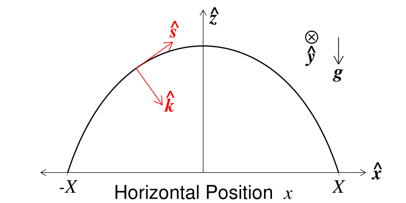
Figure 1: The geometry of the coronal loop, with the loop’s axis shown in black. The photosphere corresponds to the $x$–$y$ plane, while the loop is confined to the $x$–$z$ plane. The $y$-axis points into the page. The local Frenet coordinates are indicated in red. The local tangent vector is $\hat{s}$ and the principle normal $\hat{k}$ lies in the direction of curvature. The binormal is everywhere constant and pointed in the $\hat{y}$ direction.

In addition to the Cartesian coordinate system, both within the fibril and within the external corona we will employ the local Frenet coordinates for a field line (illustrated in Figure 1). The direction tangent to the magnetic field will be denoted with the unit vector $\hat{s}$ (thus ${\mbox{{\boldmath$B$}}}_{\rm e}=B_{\rm e}{\mbox{{\boldmath$\hat{s}$}}}$), and the longitudinal coordinate $s$ is the pathlength along a field line measured from the photosphere ($s=0$ corresponds to the footpoint intersecting the photosphere in the region $x<0$). The curvature vector for the field line is indicated by $k$, and points in the direction of the principle normal $\hat{k}$ with a modulus equal to the reciprocal of the local radius of curvature $R$ of the field line. The direction of the unit vector in the binormal direction will be indicated with $\hat{q}$ and the torsion of the field line with the variable $\tau$. In the equilibrium considered here, the loop itself lacks torsion, $\tau=0$, and its binormal uniformly points in the $y$-direction, ${\mbox{{\boldmath$\hat{q}$}}}={\mbox{{\boldmath$\hat{y}$}}}$. However, the exterior coronal magnetic field may be 3-D (with spatial symmetries near the loop). Therefore, for completeness and to aid follow-up work we consider the more general case for the moment and specialize only as necessary. The standard geometrical relations between these coordinate vectors, i.e., the Frenet-Serret formulae, are given below for reference, assuming that the position vector of a field line is given by ${\mbox{{\boldmath$r$}}}(s,t)$,

$$\hat{s} \equiv \frac{\partial{{\mbox{{\boldmath$r$}}}}}{\partial{s}}\;,$$ (2.2)

$$k \equiv \frac{\partial{{\mbox{{\boldmath$\hat{s}$}}}}}{\partial{s}}=\frac{{\mbox{{\boldmath$\hat{k}$}}}}{R}\;,$$ (2.3)

$$\hat{q} \equiv {\mbox{{\boldmath$\hat{s}$}}}\times{\mbox{{\boldmath$\hat{k}$}}}\;,$$ (2.4)

$$\frac{\partial{{\mbox{{\boldmath$\hat{k}$}}}}}{\partial{s}} = -\frac{{\mbox{{\boldmath$\hat{s}$}}}}{R}+\tau{\mbox{{\boldmath$\hat{q}$}}}\;,$$ (2.5)

$$\frac{\partial{{\mbox{{\boldmath$\hat{q}$}}}}}{\partial{s}} = -\tau{\mbox{{\boldmath$\hat{k}$}}}\;.$$ (2.6)

Notice the lack of ‘e’ subscripts on the Frenet vectors. For a sufficiently thin tube the Frenet vectors will be nearly constant across the fibril with the same value as the surrounding corona. Therefore, we avoid appending subscripted labels to the Frenet vectors of the external field to simplify notation and to emphasize that the field lines have the same direction and shape inside and immediately outside the fibril.

2.1 Cross-Sectional Averaging of the MHD Momentum Equation

The forces acting on an isolated, thin, magnetic fibril embedded in a field-free atmosphere have been previously derived by a variety of authors (Spruit, 1981; Choudhuri, 1990; Cheng, 1992) through averaging of the MHD momentum equation over the cross-sectional area of the tube. Here we rederive the equilibrium forces in the presence of a magnetized external atmosphere. Following Spruit (1981), we begin by averaging the MHD momentum equation over the cross-section of the fibril, with the goal of deriving an equation which describes the force per unit length along the fibril. In equilibrium, there will be a balance of these forces, and this balance will specify the shape of the fibril and its thermodynamic properties.

Let $A(s)$ be a cross-sectional surface of the fibril at the location $s$ that is everywhere perpendicular to the magnetic field (i.e., perpendicular to $\hat{s}$) and let $da$ be a differential area of this surface. We define the cross-sectional average of a general quantity $f$ in the natural way,

$$\bar{f}(s)\equiv\frac{1}{A(s)}\int\limits_{\!A(s)}\!\!\int f\,da\;.$$ (2.7)

We write the MHD momentum equation using a formulation of the Lorentz force that directly acknowledges that the magnetic force is transverse to the field itself,

$$\rho\frac{D{\mbox{{\boldmath$v$}}}}{Dt}=-{\mbox{{\boldmath$\nabla$}}}{P}-{\mbox{{\boldmath$\nabla$}}}_{\perp}\left(\frac{B^{2}}{8\pi}\right)+\frac{B^{2}}{4\pi}{\mbox{{\boldmath$k$}}}+{\mbox{{\boldmath$g$}}}\rho\;,$$ (2.8)

where

$${\mbox{{\boldmath$\nabla$}}}_{\perp}\equiv{\mbox{{\boldmath$\hat{k}$}}}({\mbox{{\boldmath$\hat{k}$}}}\cdot{\mbox{{\boldmath$\nabla$}}})+{\mbox{{\boldmath$\hat{q}$}}}({\mbox{{\boldmath$\hat{q}$}}}\cdot{\mbox{{\boldmath$\nabla$}}}).$$ (2.9)

In equation (2.8), the gas pressure, magnetic-field strength, and mass density within the loop are $P$, $B$, and $\rho$, respectively and $D/Dt$ denotes the Lagrangian time derivative.

We average equation (2.8) over the cross-section $A$, and seek a static solution by setting the acceleration to zero,

$$-\frac{1}{A}\int\limits_{~{}~{}A}\!\!\!\!\int\left[{\mbox{{\boldmath$\nabla$}}}P+{\mbox{{\boldmath$\nabla$}}}_{\perp}\left(\frac{B^{2}}{8\pi}\right)\right]\,da+\frac{\overline{B^{2}{\mbox{{\boldmath$k$}}}}}{4\pi}+{\mbox{{\boldmath$g$}}}\bar{\rho}=0\;.$$ (2.10)

The two terms involving gradients can be expressed as contour integrals around $\partial A$, the boundary of $A$, by using the 2-D form of the divergence theorem appropriate for integration over an open surface,

$$-\frac{1}{A}\oint\limits_{\partial A}\left(P+\frac{B^{2}}{8\pi}\right){\mbox{{\boldmath$\hat{n}$}}}\,dl-\overline{\frac{\partial{P}}{\partial{s}}{\mbox{{\boldmath$\hat{s}$}}}}+\frac{\overline{B^{2}{\mbox{{\boldmath$k$}}}}}{4\pi}+{\mbox{{\boldmath$g$}}}\bar{\rho}=0\;.$$ (2.11)

The unit vector $\hat{n}$ is the outward normal to the tube’s bounding surface. The differential $dl$ is the differential pathlength around $\partial A$. In deriving this equation, we have decomposed the gradient of the gas pressure into longitudinal and transverse components,

$${\mbox{{\boldmath$\nabla$}}}P=\frac{\partial{P}}{\partial{s}}\,{\mbox{{\boldmath$\hat{s}$}}}+{\mbox{{\boldmath$\nabla$}}}_{\perp}P\;.$$ (2.12)

The total pressure must be continuous across the loop’s bounding surface. Therefore, on $\partial A$

$$P+\frac{B^{2}}{8\pi}=P_{\rm e}+\frac{B_{\rm e}^{2}}{8\pi}\;,$$ (2.13)

and the pressures that appear within the integrand of the contour integral in equation (2.11) may be replaced with those from the external fluid,

$$-\frac{1}{A}\oint\limits_{\partial A}\left(P_{\rm e}+\frac{B_{\rm e}^{2}}{8\pi}\right){\mbox{{\boldmath$\hat{n}$}}}\,dl-\overline{\frac{\partial{P}}{\partial{s}}{\mbox{{\boldmath$\hat{s}$}}}}+\frac{\overline{B^{2}{\mbox{{\boldmath$k$}}}}}{4\pi}+{\mbox{{\boldmath$g$}}}\bar{\rho}=0\;.$$ (2.14)

Buoyancy is the sum of the gravity acting on a body and the net gas-pressure force acting on the outer surface of the body. In this case, we also must consider the effects of the external magnetic pressure and magnetic tension. We can construct an extension of Archimedes’ principle that is relevant for our problem by performing a similar cross-sectional average of the MHD momentum equation in the exterior fluid. This requires that we assume that the mathematical form of the external pressures and density can be analytically continued inside the loop. The transverse component of the resulting equation provides an expression for the net external pressure force,

$$-\frac{1}{A}\oint\limits_{\partial A}\left(P_{\rm e}+\frac{B_{\rm e}^{2}}{8\pi}\right){\mbox{{\boldmath$\hat{n}$}}}\,dl=-\frac{\overline{B_{\rm e}^{2}{\mbox{{\boldmath$k$}}}}}{4\pi}-\overline{\rho_{\rm e}{\mbox{{\boldmath$g$}}}_{\perp}}\;,$$ (2.15)

where ${\mbox{{\boldmath$g$}}}_{\perp}={\mbox{{\boldmath$g$}}}-\left({\mbox{{\boldmath$g$}}}\cdot{\mbox{{\boldmath$\hat{s}$}}}\right){\mbox{{\boldmath$\hat{s}$}}}$ is the component of $g$ perpendicular to $\hat{s}$. Since we have assumed that the tube is thin, to lowest order in the radius of the tube, the tangent vector and curvature vector are constant across a cross-section. Thus, the previous equation can be rewritten,

$$-\frac{1}{A}\oint\limits_{\partial A}\left(P_{\rm e}+\frac{B_{\rm e}^{2}}{8\pi}\right){\mbox{{\boldmath$\hat{n}$}}}\,dl=-\frac{\overline{B_{\rm e}^{2}}}{4\pi}\,{\mbox{{\boldmath$k$}}}-\bar{\rho}_{\rm e}{\mbox{{\boldmath$g$}}}_{\perp}\;.$$ (2.16)

This expression can be used to eliminate the external pressure integrals in equation (2.14). If we once again assume that the tube is thin and the Frenet vectors do not vary significantly over the tube’s cross-section, we can replace the cross-sectional averages of the densities and pressures with their axial values to obtain

$$\left[-\frac{\partial{P}}{\partial{s}}+g_{\parallel}\rho\right]{\mbox{{\boldmath$\hat{s}$}}}+\frac{B^{2}-B_{\rm e}^{2}}{4\pi}\,{\mbox{{\boldmath$k$}}}+\left(\rho-\rho_{\rm e}\right){\mbox{{\boldmath$g$}}}_{\perp}=0\;.$$ (2.17)

where $g_{\parallel}={\mbox{{\boldmath$g$}}}\cdot{\mbox{{\boldmath$\hat{s}$}}}$ is the tangential component of gravity. For simplicity we have labeled the axial values without accents or subscripts and the external magnetic field and density are to be evaluated at the location of the magnetic fibril. Note, this equation is very general; we did not assume that either of the internal or external fields were force free, nor did we assume that the loop is torsionless. Therefore, this equation is valid for a fibril that describes a fully 3-D curve through an equilibrium atmosphere filled with a general 3-D external magnetic field. The term in square brackets is the longitudinal component and represents hydrostatic balance along field lines. The remaining terms are transverse and correspond to the magnetic and buoyancy forces. In some ways these two transverse terms are analogous; the last term, buoyancy, is a combination of gravity and the net support provided by the external gas pressure, whereas the second term, the magnetic force, is the residual Lorentz force that remains once magnetic tension and the net support provided by the external magnetic pressure have been combined. Both forces are normal to the surface of the tube. Our intuition may tell us that buoyancy is aligned with gravity; but, this is only true for bodies with closed symmetric surfaces, such as a sphere. Further, just as buoyancy can point upwards or downwards depending on whether the fibril is over- or underdense, the net magnetic force can point up or down depending on the relative strength of the magnetic field inside and outside the fibril.

2.2 The Equilibrium Shape of the Fibril

We now invoke the assumption that the fibril is torsionless ($\tau=0$) and vertically oriented, therefore lacking forces in the binormal direction. Under this assumption we can separate the mean force equation (2.17) into only two components,

$$\frac{\partial{P}}{\partial{s}} = -g\rho\left({\mbox{{\boldmath$\hat{z}$}}}\cdot{\mbox{{\boldmath$\hat{s}$}}}\right)\;,$$ (2.18)

$$\frac{B^{2}-B_{\rm e}^{2}}{4\pi}R^{-1} = g\left(\rho-\rho_{\rm e}\right)({\mbox{{\boldmath$\hat{z}$}}}\cdot{\mbox{{\boldmath$\hat{k}$}}})\;.$$ (2.19)

where we have used ${\mbox{{\boldmath$g$}}}_{\perp}=({\mbox{{\boldmath$g$}}}\cdot{\mbox{{\boldmath$\hat{k}$}}}){\mbox{{\boldmath$\hat{k}$}}}$, which holds in equilibrium when the fibril is confined to the $x$–$z$ plane.

Equation (2.18) expresses the balance of forces in the tangential or axial direction $\hat{s}$, whereas equation (2.19) describes the balance in the transverse direction of the principle normal $\hat{k}$. The axial equation is simply hydrostatic balance along magnetic field lines. The transverse equation constrains the density contrast, $\rho-\rho_{\rm e}$, through the balance of magnetic and buoyancy forces. This balance can be characterized by a magnetic Bond number (Jain & Hindman, 2012),

$$\varepsilon\equiv 4\pi gX\frac{\rho-\rho_{\rm e}}{B^{2}-B_{\rm e}^{2}}\,$$ (2.20)

which is a nondimensional ratio of the buoyancy to the magnetic forces. The length scale that we have used in this definition, $2X$, is the footpoint separation, where $x=\pm X$ is the location of each of the fibril’s footpoints in the photosphere. The magnetic Bond number appears in calculations of the Rayleigh-Taylor instability when one or more of the fluid layers are filled with a horizontal field, providing the critical wavenumber below which instability ensues (Chandrasekhar, 1961).

Equation (2.19) expresses a condition on the radius of curvature $R$ of the fibril’s axis in terms of the magnetic Bond number $\varepsilon$ and the geometry of the fibril (i.e., the direction of the principle normal relative to gravity ${\mbox{{\boldmath$\hat{z}$}}}\cdot{\mbox{{\boldmath$\hat{k}$}}}$),

$$R^{-1}=\frac{\varepsilon}{X}({\mbox{{\boldmath$\hat{z}$}}}\cdot{\mbox{{\boldmath$\hat{k}$}}})\;.$$ (2.21)

To proceed we need expressions for the Frenet unit vectors, $\hat{s}$ and $\hat{k}$, the radius of curvature, $R$, and the arclength, $s$. If $z_{0}(x)$ is the height of the fibril above the photosphere, given as a function of the horizontal coordinate $x$, and the fibril’s axis is traced by the position vector ${\mbox{{\boldmath$r$}}}(x)=x\,{\mbox{{\boldmath$\hat{x}$}}}+z_{0}(x)\,{\mbox{{\boldmath$\hat{z}$}}}$, these quantities can be easily derived from equations (2.2) and (2.3),

$$\hat{s} = \frac{{\mbox{{\boldmath$\hat{x}$}}}+z_{0}^{\prime}(x){\mbox{{\boldmath$\hat{z}$}}}}{s^{\prime}(x)}\;,$$ (2.22)

$$k = -z_{0}^{\prime\prime}(x)\,\frac{z_{0}^{\prime}(x){\mbox{{\boldmath$\hat{x}$}}}-{\mbox{{\boldmath$\hat{z}$}}}}{s^{\prime}(x)^{4}}\;,$$ (2.23)

$$R(x) \equiv \left|{\mbox{{\boldmath$k$}}}\right|^{-1}=\frac{s^{\prime}(x)^{3}}{\left|z_{0}^{\prime\prime}(x)\right|}\;,$$ (2.24)

$$s^{\prime}(x) = \sqrt{1+z_{0}^{\prime}(x)^{2}}\;,$$ (2.25)

where primes denote differentiation with respect to the photospheric coordinate $x$. If we insert equations (2.23) and (2.24) into equation (2.21), we obtain a nonlinear ODE for the height of the fibril $z_{0}(x)$,

$$\frac{z_{0}^{\prime\prime}(x)}{1+z_{0}^{\prime}(x)^{2}}=\frac{\varepsilon}{X}\;.$$ (2.26)

A quick examination of this equation reveals that the fibril will be locally concave or convex depending on the sign of the magnetic Bond number and that points of inflection correspond to vanishing magnetic Bond number. The magnetic Bond number is proportional to the signed curvature. A stable fibril with a single concave arch will have a negative Bond number everywhere, whereas a multi-arched structure will have a magnetic Bond number that changes sign.

2.3 Thermodynamics of the Fibril

The temperature, density and gas pressure within the loop can all differ from the surrounding corona. We define the contrasts is these properties in the following manner:

$$\Delta\rho(s) \equiv \rho(s)-\rho_{\rm e}(s)\;,$$ (2.27)

$$\Delta P(s) \equiv P(s)-P_{\rm e}(s)\;,$$ (2.28)

$$\Delta T(s) \equiv T(s)-T_{\rm e}(s)\;.$$ (2.29)

Technically the external variables are all functions of two spatial coordinates—e.g., $x$ and $z$. In all of these definitions, however, the external variable is evaluated at the location of the fibril. We indicate this by expressing these variables as a function of the pathlength alone. Only the contrasts in the mass density $\Delta\rho$, gas pressure $\Delta P$, and magnetic pressure $\Delta B^{2}/8\pi$ play an active role in the force balance. The temperature contrast $\Delta T$ is a dependent variable that can be derived from these active variables post facto. There are four primary equations that provide all of the inter-relations between these properties of the loop,

$${\textstyle\rm Pressure~{}Continuity}\qquad\displaystyle\Delta P = -\frac{\Delta B^{2}}{8\pi}\;,$$ (2.30)

$${\textstyle\rm Hydrostatic~{}Balance}\quad\;\displaystyle\frac{d{\Delta P}}{d{z_{0}}} = -g\Delta\rho\;,$$ (2.31)

$${\textstyle\rm Transverse~{}Force~{}Balance}\qquad\quad\displaystyle\frac{\varepsilon}{X} = -\frac{g}{2}\,\frac{\Delta\rho}{\Delta P}=\frac{z_{0}^{\prime\prime}}{1+(z_{0}^{\prime})^{2}}\;,$$ (2.32)

$${\textstyle\rm Field~{}Strength~{}Deviation}\quad\;\displaystyle\frac{\Delta B^{2}}{8\pi} = \alpha\frac{B_{\rm e}^{2}}{8\pi}\;.$$ (2.33)

The first of these is a direct consequence of equation (2.13). The second results from transforming equation (2.18) from the pathlength variable $s$ to the fibril height $z_{0}$. The third relation, equation (2.32), arises from a combination of the definition of the magnetic Bond number (2.20) and the equation of transverse force balance (2.26), where the magnetic-pressure contrast has been replaced through use of pressure continuity, equation (2.30). The last equation is a restatement of equation (2.1) which ensures that loop and external magnetic field share a common bounding flux surface. The temperature contrast $\Delta T$ can be found by using the ideal gas law ($P=R_{\rm gas}\rho T$),

$$\Delta T=\frac{g(h-H_{\rm e})}{R_{\rm gas}}\frac{\Delta\rho}{\rho}\;,$$ (2.34)

where $H_{\rm e}$ is the external corona’s pressure scale height, $H_{\rm e}=R_{\rm gas}T_{\rm e}/g$, and $h$ is the scale height of the gas-pressure contrast,

$$h^{-1}\equiv-\frac{2\varepsilon}{X}=-\frac{1}{\Delta P}\frac{d{\Delta P}}{d{z_{0}}}\;.$$ (2.35)

Conveniently, these equations can be solved analytically to obtain the contrast variables as a function of the fibril’s shape. If we combine equations (2.31) and (2.32), we obtain a differential equation that relates the pressure contrast to the derivative of the fibril’s height,

$$\frac{1}{\Delta P}\frac{d{\Delta P}}{d{z_{0}}}=\frac{2z_{0}^{\prime\prime}(x)}{1+z_{0}^{\prime}(x)^{2}}\;.$$ (2.36)

This equation can be directly integrated to obtain,

$$\Delta P=-\alpha C\left[1+(z_{0}^{\prime})^{2}\right]\;,$$ (2.37)

where $C$ is a positive integration constant that can be fixed in a variety of ways. One could apply a photospheric boundary condition or one could use spectroscopic observations to fix the temperature or density contrast at the apex of the loop. Strictly speaking, the integration constant is the product $\alpha C$. We have included the field-strength deviation in this product for later convenience and in order to remind the reader that the thermodynamic contrasts arise from a small deviation from the force-free equilibrium. If we subsequently use the equations of pressure continuity (2.30) and hydrostatic balance (2.31), we can derive equations for the mass density and magnetic-pressure contrasts,

$$\Delta\rho = \frac{2\alpha C}{g}z_{0}^{\prime\prime}\;,$$ (2.38)

$$\frac{\Delta B^{2}}{8\pi} = \alpha C\left[1+(z_{0}^{\prime})^{2}\right]\;.$$ (2.39)

Thus, if we are provided the shape of the loop, we can derive all of the loop’s contrast variables. Different values of the integration constant $\alpha C$ result in different temperature profiles along the loop. Equation (2.34) can be rewritten to show how the temperature contrast depends on the geometry of the loop and the constant $\alpha C$,

$$\Delta T=-\alpha CT_{\rm e}\,\frac{\left[1+(z_{0}^{\prime})^{2}+2H_{\rm e}z_{0}^{\prime\prime}\right]}{P_{\rm e}+2\alpha CH_{\rm e}z_{0}^{\prime\prime}}\;.$$ (2.40)

Note that the integration constant $C$ was chosen such that it appears only in the combination of $\alpha C$ in the equations above. Thus, one needs only a single constraint to define the thermodynamic variables.

2.4 Self-Consistent External Magnetic Field

Given the pressure contrast $\Delta P$, we can use equations (2.30), (2.33), and (2.37) to express the external field strength at the location of the fibril in terms of the geometry of the fibril,

$$\frac{B_{\rm e}^{2}(s)}{8\pi}=C\left[1+(z_{0}^{\prime})^{2}\right]\;.$$ (2.41)

This last equation shows that the integration constant $C$ is really just the value of the external magnetic pressure at the apex of the loop (hence $C$ is positive). Further, the equation demonstrates that not all external fields are self-consistent with an embedded fibril. If we select an arbitrary field line within a general magnetic field, equation (2.41) may not be satisfied for a constant $C$. This becomes readily apparent when we express the direction of the tangent vector in terms of the angle $\theta$ that it makes with the $x$-axis, ${\mbox{{\boldmath$\hat{s}$}}}\equiv\cos\theta\,{\mbox{{\boldmath$\hat{x}$}}}+\sin\theta\,{\mbox{{\boldmath$\hat{z}$}}}$. With a little basic manipulation, we find the following relation between the angle $\theta$ and the height function $z_{0}$:

$$\sec^{2}\theta=1+(z_{0}^{\prime})^{2}\;.$$ (2.42)

Subsequently, one can easily show that equation (2.41) is equivalent to the statement that the $x$-component of the external magnetic field is constant along the length of the fibril,

$${\mbox{{\boldmath$\hat{x}$}}}\cdot{\mbox{{\boldmath$B$}}}_{\rm e}=B_{\rm e}\cos\theta=\sqrt{8\pi C}\;.$$ (2.43)

Of course, not all force-free fields will have this property.

If needed, a self-consistent external magnetic field can be derived by noting that the shape of the fibril and the strength of the magnetic field at the location of the fibril provide a boundary condition for the coronal magnetic field that occupies the bulk of the domain. For simplicity we assume that the external magnetic field is potential and 2D. Therefore, since the field is solenoidal and 2D it can be described by a flux function $\Psi_{\rm e}$,

$${\mbox{{\boldmath$B$}}}_{\rm e}={\mbox{{\boldmath$\nabla$}}}\times\left(\Psi_{\rm e}{\mbox{{\boldmath$\hat{y}$}}}\right)=-\frac{\partial{\Psi_{\rm e}}}{\partial{z}}\,{\mbox{{\boldmath$\hat{x}$}}}+\frac{\partial{\Psi_{\rm e}}}{\partial{x}}\,{\mbox{{\boldmath$\hat{z}$}}}\;.$$ (2.44)

Since the field is potential the flux function must be harmonic,

$$\nabla^{2}\Psi_{\rm e}=0\;.$$ (2.45)

Therefore, we can find a self-consistent external field solution by solving equation (2.45) under the boundary condition

$${\mbox{{\boldmath$\nabla$}}}\Psi_{\rm e}=B_{\rm e}(s)\,{\mbox{{\boldmath$\hat{k}$}}}(s)\;,$$

applied at the location of the fibril with $B_{\rm e}(s)$ fixed by equation (2.41). This ensures that the external field is both parallel to the fibril and the field strength is given by $B_{\rm e}(s)$. There is an infinity of such solutions, all with different photospheric boundary conditions.

3 A Model with Uniform Magnetic Bond Number

For our first example solution we wish to consider one that is both simple and fully analytic. Therefore, we consider a fibril which has constant magnetic Bond number $\varepsilon$ along its length. For constant $\varepsilon$, the transverse force equation (2.32) can be integrated twice to obtain the height of the fibril $z_{0}(x)$. Similarly, using the result of the first of these integrations, equation (2.25) can be integrated to obtain the arclength $s(x)$. We choose the three constants of integration such that the footpoints occur at $x=\pm X$, the fibril is symmetric about $x=0$, and the footpoint at $x=-X$ corresponds to $s=0$,

$$z_{0}(\pm X)=z_{0}^{\prime}(0)=s(-X)=0\;.$$ (3.46)

With these conditions, we find the following solution for the geometrical properties of the fibril:

$$z_{0}(x) = -\frac{X}{\varepsilon}\ln\left(\frac{\cos\left(\varepsilon x/X\right)}{\cos\varepsilon}\right)\;,$$ (3.47)

$$z_{0}^{\prime}(x) = \tan\left(\varepsilon x/X\right)\;,$$ (3.48)

$$R(x) = -\frac{X}{\varepsilon}\sec\left(\varepsilon x/X\right)\;,$$ (3.49)

$$s(x) = \frac{X}{2\varepsilon}\ln\left(\frac{1+\sin\varepsilon}{1-\sin\varepsilon}\;\;\frac{1+\sin\left(\varepsilon x/X\right)}{1-\sin\left(\varepsilon x/X\right)}\right)\;.$$ (3.50)

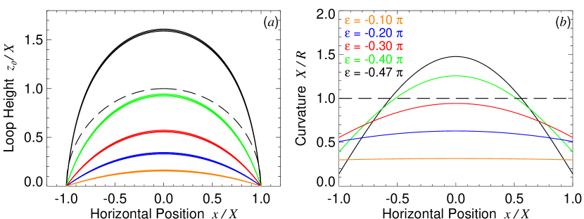
Figure 2: Equilibrium ($a$) height and ($b$) curvature of coronal loops with differing ratios of buoyancy to magnetic forces, i.e., differing values of the magnetic Bond number $\varepsilon$. The value of $\varepsilon$ associated with each color is indicated in the right panel. In both panels the dashed line corresponds to a semi-circle with constant radius of curvature $R=X$. Loops with weak buoyancy ($\left|\varepsilon\right|<<1$) are flat with large radius of curvature everywhere. Loops with substantial buoyancy ($\varepsilon\approx-\pi/2$) are tall with small curvature in the legs and large curvature at its apex. Loops with positive $\varepsilon$ or with $\varepsilon<-\pi/2$ are unstable.

Figure 2 displays solutions for several different values of $\varepsilon$. It is clear that fibril posesses a nonconstant radius of curvature, with strong curvature near the apex and weaker curvature in the legs.

The length of the fibril $L$ is obtained by inserting the rightmost footpoint position $x=X$ into equation (3.50),

$$L=\frac{X}{\varepsilon}\ln\left(\frac{1+\sin\varepsilon}{1-\sin\varepsilon}\right)\;.$$ (3.51)

Two interesting limits of this equation exist. As $\varepsilon\to 0$ the length of the loop converges to the footpoint separation $L\to 2X$. This arises because the loop becomes straight, flat, and confined to the photosphere. As $\varepsilon\to\pm\pi/2$ the loop length diverges logarithmically because the height of the loop grows without bound. This can be seen by recognizing that the loop reaches its apex at its center ($x=0$), therefore achieving a maximum height of

$$z_{\rm apex}=z_{0}(0)=\frac{X}{\varepsilon}\ln\left(\cos\varepsilon\right)\;.$$ (3.52)

One can easily see that $\varepsilon=\pm\pi/2$ corresponds to a logarithmic singularity in the height. Clearly the height $z_{0}(x)$ should be a positive function for the range $x\in(-X,~{}X)$. With a little thought, from equation (3.47) we can see that this is only possible if $\varepsilon\in(-\pi/2,0)$, once again emphasizing that a fibril with a single concave arch has a negative magnetic Bond number.

3.1 Thermodynamics of a Fibril with Uniform Magnetic Bond Number

The contrast variables have a common geometrical factor, $1+(z_{0}^{\prime})^{2}$, appearing in their functional forms. For the model with uniform magnetic Bond number this factor takes on a simple form. Using equations (3.47) and (3.48), we find

$$1+(z_{0}^{\prime})^{2}=\sec^{2}\left(\varepsilon x/X\right)=\sec^{2}\varepsilon\;\exp\left(-z_{0}/h\right)\;.$$ (3.53)

Using this expression and the equations derived in subsection §2.3 we can solve for all of the contrast variables and the external magnetic pressure in terms of the scale height $h$ that depends on the Bond number, $h=-X/2\varepsilon$,

$$\Delta P = -\frac{\Delta B^{2}}{8\pi}=-\alpha C\,\exp\left(\frac{z_{\rm apex}-z_{0}}{h}\right)\;,$$ (3.54)

$$\Delta\rho = -\frac{\alpha C}{gh}\,\exp\left(\frac{z_{\rm apex}-z_{0}}{h}\right)\;,$$ (3.55)

$$\Delta T = T_{\rm e}\left(\frac{h}{H_{\rm e}}-1\right)\frac{\Delta\rho}{\rho_{\rm e}+\Delta\rho_{\rm e}}\;,$$ (3.56)

$$\frac{B_{\rm e}^{2}}{8\pi} = C\,\exp\left(\frac{z_{\rm apex}-z_{0}}{h}\right)\;.$$ (3.57)

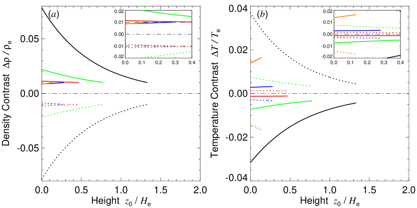
Figure 3: Fractional ($a$) mass density and ($b$) temperature contrast as a function of height for loops with constant magnetic Bond number and a footpoint separation of $2X=250$ Mm. The external atmosphere is isothermal with a scale height of $H_{\rm e}=75$ Mm. The different colors indicate different Bond numbers with the same color coding as in Figure 2. For all loops, the fractional density contrast has been set to a value of $\Delta\rho/\rho_{\rm e}=\pm 0.01$ at the loop’s apex. The solid curves are for overdense loops $\Delta\rho>0$ and the dotted curves are for underdense loops $\Delta\rho<0$. Overdense loops correspond to loops that have been heated and undedense loops to those that have been cooled. Clearly, overdense loops are more physically relevant. The dot-dashed curve is a reference line for vanishing contrast. The insets display zoom-in views designed to highlight short loops with small magnetic Bond number. In the mass density inset, the dashed horizontal lines indicate the values of the contrast fixed at the apex. The contrasts decrease in magnitude with height for loops with $H_{\rm e}<h$ and increase in magnitude for loops with $H_{\rm e}>h$, where $h$ is the scale height for the contrast variables. For the illustrated values of the magnetic Bond number, $h$ ranges from 34 Mm to 160 Mm, with the black curve ($\varepsilon=-0.47\,\pi$) having the smallest value and the orange curve ($\varepsilon=-0.1\,\pi$) the largest. The blue curve has $h=1.06~{}H_{\rm e}$, thus sitting near the transition between the two behaviors.

The density and pressure contrasts, as well as the external magnetic pressure, are revealed to be exponential functions of height, all with the same constant scale height $h$. The density and temperature contrast are illustrated in Figure 3, for an isothermal exterior with a scale height of $H_{\rm e}=75$ Mm. The constant $\alpha C$ has been chosen such that the fractional density contrast at the apex of the loop is $\Delta\rho/\rho_{\rm e}=\pm 0.01$. The solid curves correspond to overdense loops and the dotted curves to underdense loops, with the different colors corresponding to loops with different magnetic Bond numbers. We will see in the discussion section §5 that overdense loops have been heated relative to the surrounding corona and underdense loops have been cooled. Therefore, overdense loops are probably more physically relevant.

For an isothermal exterior, where $H_{\rm e}$ is a constant, one could choose the magnetic Bond number such that $h=H_{\rm e}$. For such a model, the temperature contrast would be identically zero all along the length of the loop and the plasma parameter $\beta=8\pi P/B^{2}$ would be a constant both inside and outside the loop, while the density contrast remains nonzero. The condition $H_{\rm e}=h$ marks a transition between disparate behavior. Loops with $H_{\rm e}<h$ have fractional density and temperature contrasts that decrease with height, whereas loops with $H_{\rm e}>h$ have fractional density and temperature contrasts that increase with height.

3.2 A Self-Consistent External Magnetic Field

In the previous subsection we discovered that a fibril with constant magnetic Bond number requires that the external magnetic pressure have a constant scale height as we slide along the fibril. This suggests that we seek a solution in which the magnetic pressure is only a function of height and varies exponentially. A simple harmonic solution that satisfies this requirement is a sinusoid in the horizontal $x$-direction multiplied by a decaying exponential in height $z$,

$$\Psi_{\rm e}(x,z)=\kappa^{-1}\,\tilde{B}_{\rm e}\cos(\kappa x)\,e^{-\kappa z}\;.$$ (3.58)

In this solution, $2\pi/\kappa$ is the horizontal repetition length of the field ($\Psi_{\rm e}$ changes sign every $\pi/\kappa$). With such a flux function, the magnetic field is as follows:

$${\mbox{{\boldmath$B$}}}_{\rm e}(x,z)=\tilde{B}_{\rm e}\left[\cos(\kappa x){\mbox{{\boldmath$\hat{x}$}}}-\sin(\kappa x){\mbox{{\boldmath$\hat{z}$}}}\right]\,e^{-\kappa z}\;.$$ (3.59)

Since the magnetic field is periodic in the $x$-direction, we will only consider the arcade that is symmetric about the origin and exists in the range $x\in(-D,D)$, where $D=\pi/(2\kappa)$. The magnetic pressure for such a field depends only on height and falls off exponentially with a scale height of $(2\kappa)^{-1}$,

$$\frac{B_{\rm e}^{2}}{8\pi}=\frac{\tilde{B}_{\rm e}^{2}}{8\pi}\,e^{-2\kappa z}\;.$$ (3.60)

In order to satisfy equation (3.57), we must insist that the external field’s horizontal wavenumber is proportional to the magnetic Bond number and that the photospheric value of the field strength depends on $C$,

$$\kappa = -\frac{\varepsilon}{X}=\frac{2}{h}\;,$$ (3.61)

$$\frac{\tilde{B}_{\rm e}}{8\pi} = C\exp\left(\frac{z_{\rm apex}}{h}\right)\;.$$ (3.62)

Lines of constant $\Psi_{\rm e}$ in the $x$–$z$ plane denote field lines. The height above the photosphere, $z_{\rm e}$, of a field line with a specified value of the flux function is easily obtained by inverting equation (3.58),

$$z_{\rm e}(x;\Psi_{\rm e})=\kappa^{-1}\ln\left(\frac{\cos(\kappa x)}{\cos(\kappa x_{\Psi})}\right)\;,$$ (3.63)

where the footpoints intersect the photosphere at $x=\pm x_{\Psi}$,

$$x_{\Psi}\equiv\kappa^{-1}\cos^{-1}\left(\frac{\kappa\Psi_{\rm e}}{\tilde{B}_{\rm e}}\right)\;.$$ (3.64)

We can clearly see from equation (3.47) that this potential field solution for the external corona is consistent with the loop model, equation, if the magnetic Bond number is inversely proportional to the repetition length of the external magnetic field, $\varepsilon=-\kappa X$, which is a condition we have already imposed to ensure that the external field strength has the appropriate value along the fibril.

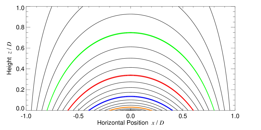
Figure 4: Field lines for a potential corona with embedded magnetic fibrils, all with constant magnetic Bond number. The coronal field (black lines) was constructed from a harmonic solution, with a single wavenumber, $\kappa=\pi/(2D)$, in the $x$-direction—see equation (3.58). The colored field lines indicate magnetic fibrils with different magnetic Bond numbers with the same color coding as Figure 2 (green: -0.4 $\pi$, red: -0.3 $\pi$, blue: -0.2 $\pi$, and orange: -0.1 $\pi$).

The field lines of this potential field are illustrated in Figure 4. In the beginning of this section we discovered that stability requires that the magnetic Bond number be bounded $\varepsilon\in(-\pi/2,0)$. In the context of this specific model, we can see that the magnetic Bond number selects the field line within the coronal field that corresponds to the axis of the fibril. Fibrils with different footpoint separations and magnetic Bond numbers are shown as various colored field lines in Figure 4. A small value of the magnetic Bond number corresponds to a short, flat, low-lying loop confined very near the origin, while a magnetic Bond number near the lower limit is a tall, long loop, with foot-points approaching the outer edge of the arcade. In fact, in the limit $\varepsilon\to-\pi/2$, the loop is infinitely tall with vertical legs located at $x=\pm X=\pm D$. Therefore, there is a direct mapping between the magnetic Bond number and the value of the flux function that corresponds to the loop’s axis,

$$\Psi_{\rm fibril}=(2D/\pi)\,\tilde{B}_{\rm e}\cos\varepsilon=h\sqrt{\frac{\pi C}{2}}\;,$$ (3.65)

and one can choose to place the loop along any field line in the coronal model by dialing the magnetic Bond number between $-\pi/2$ and 0.

4 A Model with Uniform Radius of Curvature

Another simple model to consider is a fibril with a constant radius of curvature. This model is of course an example of a fibril with a nonuniform magnetic Bond number. However, it is still a single concave arch and therefore the Bond number will be negative everywhere. With a constant radius of curvature $R$, equation (2.21) simplifies to

$$\varepsilon=-\frac{X}{z_{0}-z_{c}}\;,$$ (4.66)

where $z_{c}$ is the height above the photosphere of the fibril’s center of curvature. From this expression we can see that the magnetic Bond number diverges when $z_{0}=z_{c}$ resulting in a divergence of all the contrast variables at the same location. Therefore, for a physically meaningful solution we must insist that the center of curvature lies below the photosphere, i.e., $z_{c}<0$. The fibril is therefore a circular arc that is less than a full semi-circle and intersects the photosphere at oblique angles.

Using the procedure outlined in subsection §2.3 we derive all of the contrast variables and the external magnetic pressure from the magnetic Bond number,

$$\Delta P = -\alpha C\left(\frac{R}{z_{0}-z_{c}}\right)^{2}\;,$$ (4.67)

$$\Delta\rho = -\frac{2\alpha C}{gR}\,\left(\frac{R}{z_{0}-z_{c}}\right)^{3}\;,$$ (4.68)

$$\Delta T = T_{\rm e}\,\left(\frac{z_{0}-z_{c}}{2H_{\rm e}}-1\right)\frac{\Delta\rho}{\rho_{\rm e}+\Delta\rho}\;,$$ (4.69)

$$\frac{B_{\rm e}^{2}}{8\pi} = C\,\left(\frac{R}{z_{0}-z_{c}}\right)^{2}\;.$$ (4.70)

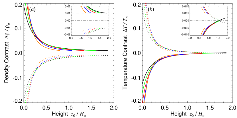
Figure 5: Fractional ($a$) mass density and ($b$) temperature contrast as a function of height for loops with constant radius of curvature. The external atmosphere is isothermal with a scale height of $H_{\rm e}=75$ Mm. The different colors indicate loops with different radii of curvature (black: $R=175$ Mm, green: 150 Mm, red: 125 Mm, blue: 100 Mm, orange: 75 Mm). For all loops, the fractional density contrast has been set to a value of $\Delta\rho/\rho_{\rm e}=\pm 0.01$ at the loop’s apex. The solid curves are for overdense loops $\Delta\rho>0$ (heated loops) and the dotted curves are for underdense loops $\Delta\rho<0$ (cooled loops). The dot-dashed curve is a reference line for vanishing contrast and the dashed curves in the inset correspond to the apex values. The contrasts generally decrease in magnitude with height. However, loops of sufficient size, $R>2H_{\rm e}$, can have a temperature inversion at their apex (see the inset in panel $b$).

Figure 5 illustrates the density and temperature contrasts for loops with radii of curvature spanning 25–125 Mm. Each is embedded in an isothermal corona with a scale height of 75 Mm. The integration constant $\alpha C$ has been chosen such that the fractional density contrast is $\Delta\rho/\rho_{\rm e}=\pm 0.01$ at the apex of the loop. For all of the loops the magnitude of the density contrast decreases with height. For the parameters chosen for the figure, the overdense loops tend to be cold compared to their surroundings, although those that are sufficiently large ($R>2H_{\rm e}$) can have a warm crest. Similarly, underdense loops tend to be hot with the tallest and widest loops possessing a cool crest. If a change of sign occurs, it will happen at a distance of two scale heights above the center of curvature.

Many external field solutions could be found that possess circular field lines; however, most will not possess the needed functional form for the external field strength along the loop. Consider the field generated by a line current located at the center of curvature. Such a line current generates a field with concentric field lines that have constant field stength as one moves along a line. We can see that this field fails because equation (4.70) dictates that the field strength must decrease with height along the fibril. The functional form for $B_{\rm e}$ given by that equation and the fact that the fibril is a circular arc, suggests that we seek a solution in polar coordinates with the following form,

$$\Psi_{\rm e}(r,\phi) = \tilde{B}_{\rm e}\,\frac{z_{c}}{R}\,\frac{r-R}{\sin\phi}\;,$$ (4.71)

$${\mbox{{\boldmath$B$}}}_{\rm e} = \frac{1}{r}\frac{\partial{\Psi_{\rm e}}}{\partial{\phi}}\,{\mbox{{\boldmath$\hat{r}$}}}-\frac{\partial{\Psi_{\rm e}}}{\partial{r}}\,{\mbox{{\boldmath$\hat{\phi}$}}}$$

$$= -\frac{z_{c}}{R}\,\frac{\tilde{B}_{\rm e}}{\sin^{2}\phi}\left(\frac{r-R}{r}\,\cos\phi\,{\mbox{{\boldmath$\hat{r}$}}}+\sin\phi\,{\mbox{{\boldmath$\hat{\phi}$}}}\right)\;,$$

where $r^{2}=x^{2}+(z-z_{c})^{2}$ and $\sin\phi=(z-z_{c})/r$. The origin of the polar coordinate system is located at the center of curvature, $R$ is the radius of curvature of the fibril, and $\phi=0$ points in the positive $x$-direction. Once again, $\tilde{B}_{\rm e}$ is the value of the external magnetic field strength at the footpoints. We can verify that this particular potential field has a circular field line at $r=R$ by noting that the flux function is constant there (in fact, $\Psi_{\rm e}=0$ on the fibril). Direct evaluation further verifies that the magnetic pressure when evaluated at the location of the fibril has the requisite functional form, equation (4.70), as long as

$$\frac{\tilde{B}_{\rm e}^{2}}{8\pi}=\frac{CR^{2}}{z_{c}^{2}}\;.$$ (4.73)

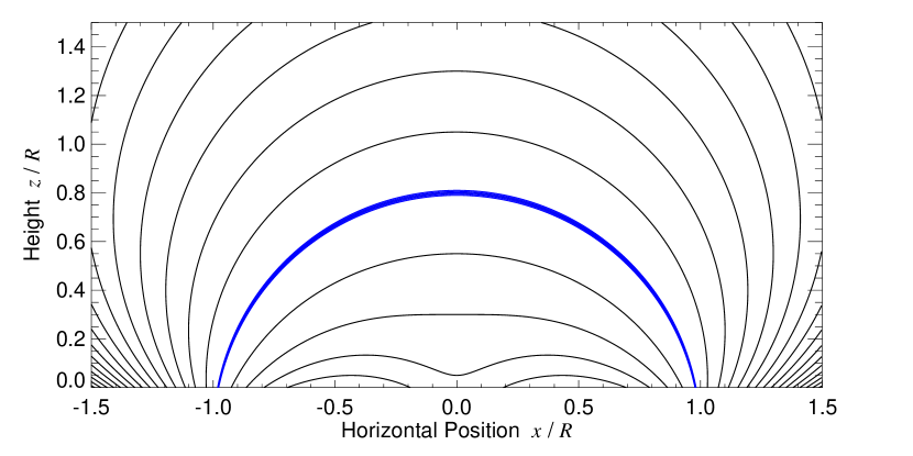
Figure 6: Field lines for a potential corona with an embedded magnetic fibril with a constant radius of curvature $R$. The field lines spread with height.

The field lines for this potential field are illustrated in Figure 6. The external field lines are drawn in black and the circular fibril is marked in blue. Note, unlike the constant magnetic Bond number model presented in section §3 where one could dial the control parameter $\varepsilon$ to change where the fibril appears in the corona, only one field line in Figure 6 meets the prerequisite of constant curvature. Thus, while self-similar, this external magnetic-field model differs for fibrils with different radii of curvature.

5 Discussion

Our equilibrium model is predicated on the implicit assumption that force balance is achieved at a much faster time scale than radiative cooling and thermal conduction redistribute heat. Hydrostatic equilibrium should be established on a dynamical time scale in between the free-fall time and the acoustic crossing time. Thus, for a loop that reaches 50 Mm above the photosphere and for a pressure scale height of 80 Mm, the dynamical time scale lies between 10–40 minutes. Transverse force balance is achieved by mass redistribution along the loop and should therefore be established on a similar time scale. Estimates of the radiative cooling and conduction times vary, but for active region loops radiative times can be on the order of 1–40 hr and conduction times are typically 1 hr (Aschwanden, 2005). Therefore, we expect that immediately after an impulsive heating event, a coronal loop will quickly re-establish force balance and will stay in force balance as the loop slowly cools. In the following section we discuss the implications of this balance.

5.1 Role of the Magnetic Bond Number

The shape of a coronal loop is determined by the force-free equilibrium of the surrounding corona. Given this shape, the mass along the loop must redistribute itself such that the buoyancy forces exactly oppose the Lorentz forces acting on the loop. The resulting balance of forces can be succinctly characterized by the magnetic Bond number which is fully specified by the height of the loop above the photosphere as a function of position. In equilibrium, the magnetic Bond number is proportional to the signed curvature of the loop, and therefore concave curvature results in a negative magnetic Bond number and convex curvature in a positive Bond number. Of course, inflection points correspond to locations where the Bond number vanishes. Therefore, a loop comprised of a single concave arch must have negative magnetic Bond number everywhere if in equilibrium. Equilibrium loops that possess multiple arches will have negative Bond number in the crests and positive Bond number in the dips or troughs.

All loops with the same geometric shape have exactly the same profile of the magnetic Bond number. However, these loops can be achieved in a continuum of different ways, all varying in the distribution of mass and field strength. This continuum is represented by different values of an integration constant $\alpha C$ which is a direct measure of the magnetic-pressure contrast at the apex of the loop. For example, an underdense loop with enhanced magnetic-field strength can have exactly the same Bond number as an overdense loop with reduced field strength. While the shape of these two loops will be the same, the thermodynamic and magnetic properties of these two loop might be very different.

5.2 Mass Redistribution along the Loop

For a loop with enhanced field strength, the mass density is proportional to the second derivative of the height function with respect to the horizontal photospheric coordinate, equation (2.38). Thus, we can immediately deduce that peaks or crests in a loop will have a mass deficit while dips or troughs have mass accumulation. Furthermore, if we define the total mass deviation between two points as the integrated density contrast,

$$\Delta M(s_{1},s_{2})\equiv\int_{s_{1}}^{s_{2}}\Delta\rho(s)\,A(s)\,ds\;,$$ (5.74)

then the mass deviation vanishes if we choose two points that correspond to extrema in height. This can be revealed by noting that flux conservation within the loop requires the following:

$$A(s)=\frac{A_{\rm apex}}{\left[1+(z_{0})^{2}\right]^{1/2}}\;,$$ (5.75)

where $A_{\rm apex}$ is the cross-sectional area of the loop at the apex. If we change variable from the pathlength to the photospheric $x$ coordinate and replace the density contrast using equation (2.38) the integral can be evaluated trivially,

$$\Delta M(x_{1},x_{2})=\frac{2\alpha CA_{\rm apex}}{g}\,\left[z_{0}^{\prime}(x_{2})-z_{0}^{\prime}(x_{1})\right]\;,$$ (5.76)

Thus, the net mass deviation between a crest and a neighboring trough is zero and the crest drains mass into the dips. For a loop comprised of a single concave arch, the mass deviation between the two footpoints is negative. Mass must drain out of the loop through the photosphere into the solar interior. In the opposite case, a loop with a reduced field strength, the mass density is proportional to the negative of the second derivative. The peaks in such a loop must have enhanced density so that buoyancy can oppose the upward Lorentz force. This obviously implies that the gas pressure must increase throughout the loop to increase the hydrostatic support. The additional mass is lifted from the photosphere into the loop.

5.3 Temperature Profile

Observations of the temperature along the length of a coronal loops have suggested that some loops might be nearly isothermal (Aschwanden et al., 2001). For the relatively small density contrasts that have been explored here, the temperature contrast is also relatively small and the temperature is perforce roughly isothermal as long as the external corona is isothermal. However, we wish to point out that the temperature contrast itself is markedly constant over height for a signficant fraction of the models we have illustrated. Three of the models with constant magnetic Bond number, appearing in Figure 3, have a temperature variation of less than a 30% percent from footpoint to apex. These three correspond to the models with the squattest loops.

Given a specific shape for a coronal loop there exists a family of possible solutions, each characterized by a different value of $\alpha C$, the integration constant—see equations (2.37)–(2.40). When illustrating our models, we chose to fix this parameter by specifying the fractional density contrast at the apex of the loop. We wish to point out, however, that the parameter $\alpha C$ is really a measure of the total heat that has been input into the coronal loop. The excess heat contained by the loop per unit length is given by

$$E(s)=c_{v}A(s)\left[\rho(s)T(s)-\rho_{\rm e}(s)T_{\rm e}(s)\right]=(\gamma-1)^{-1}A(s)\Delta P(s)\;,$$ (5.77)

where $c_{v}$ is the specific heat at constant volume and $\gamma$ is the adiabatic exponent. We can obtain the total excess heat contained by the loop by integrating $E(s)$ over the loop’s length. If we eliminate the gas-pressure contrast by using equation (2.37), we reduce the integral to a constant factor times a positive definite integral that depends only on the geometry of the loop,

$$\int_{0}^{L}E(s)\,ds=-\frac{\alpha CA_{\rm apex}}{\gamma-1}\,\int_{-X}^{X}\left[1+\left(z_{0}^{\prime}\right)^{2}\right]\,dx\;,$$ (5.78)

Since the constant $C$ and the integral appearing on the right hand side of the previous equation are always positive, we can immediately discern two facts: (1) Heated loops correspond to those with a negative field-strength deviation $\alpha$ and cooled loops to those with a positive value. Thus, heated loops are those that are undermagnetized and overdense and cooled loops are overmagnetized and underdense. (2) The integration constant $C$ is a measure of the magnitude of the heat that has been injected into or extracted from the loop. Obviously, heat deposition is more likely to be physically relevant. The family of solutions defined by different values of $C$ form a continuum of loop models with different amounts of stored heat. For example, after a large impulsive heating event, the heat content of the loop jumps but force balance is quickly re-established. This requires a redistribution of mass (and heat) along the loop and the resulting balance is characterized by a nonzero value of $C$. Then as radiative cooling and conduction slowly dissipate the loop’s excess heat, the loop responds by moving through a sequence of equilibria while simultaneously maintaining force balance. This sequence is represented by slow temporal attenuation of the parameter $C$.

5.4 Implications for Loop Seismology

Seismology of a coronal loop is only sensitive to the distribution of wave speed along the loop (e.g., Jain & Hindman, 2012). If we assume that the observed waves are kink oscillations and that they propagate at the kink speed,

$$c_{K}^{2}=\frac{B^{2}+B_{\rm e}^{2}}{4\pi(\rho+\rho_{\rm e})}\;,$$ (5.79)

then, at best, a seismic analysis can provide information about the ratio of the field strength to the density. It is impossible from only a seismic analysis to measure the field strength profile independently of the density profile. However, with additional constraints, provided either from observations or from basic physical principles, one might be able to disentangle field-strength and density variations along the loop. The force-balance model constructed here provides just such a constraint. The density contrast and magnetic-pressure contrast are related to the geometry of the loop through the magnetic Bond number,

$$\frac{\Delta B^{2}}{4\pi}=\frac{gX}{\varepsilon}\Delta\rho=gX\frac{1+(z_{0}^{\prime})^{2}}{z_{0}^{\prime\prime}}\Delta\rho\;.$$ (5.80)

If we assume that the interior magnetic field is nearly the same as the external field (hence the field-strength deviation is small), we can use this previous equation to express the kink speed solely in terms of the density contrast, the exterior density and the loop’s geometry,

$$c_{K}^{2}=2C\frac{1+(z_{0}^{\prime})^{2}}{\rho_{\rm e}+(\alpha C/g)z_{0}^{\prime\prime}}\;.$$ (5.81)

If we further assume that the exterior corona is isothermal, $\rho_{\rm e}=\tilde{\rho}_{\rm e}\exp(-z/H_{\rm e})$, this expression has only four free parameters: the integration constant $C$, the field-strength deviation $\alpha$, the coronal scale height $H_{\rm e}$ and photospheric value of the exterior density $\tilde{\rho}_{\rm e}$. Thus, even the measurement of only a few mode frequencies that provide different spatial averages of the kink speed should be sufficient to either fix these parameters or to verify a choice made using other information.

5.5 Conclusions

We have developed a model of curved coronal loops that self-consistently couples deviations from the force-free state to the thermodynamic properties. The coupling is accomplished by requiring that the loop is in equilibrium and the Lorentz force arising from the deviation from a force-free field is balanced by buoyancy. This links the curvature of the loop to the loop’s mass-density contrast and hence to the pressure and temperature through hydrostatic balance and the ideal gas law. The end result is that specification of the loop’s geometry is sufficient to derive the temperature and density profiles to within a single integration constant. This integration constant can be selected in a variety of ways, either seismically through estimates of the mean kink-wave speed or spectroscopically through estimates of the density or temperature contrast at one position along the loop. Further, this integration constant is a direct assessment of the thermal history of the loop providing an estimate of the excess heat contained by the loop relative to the surrounding corona.

References

- Aschwanden (2005) Aschwanden M. J. 2005, Physics of the Solar Corona, (Springer-Verlag: Heidelberg), pp. 321–322
- Aschwanden (2011) Aschwanden M. J. 2011, LRSP, 8, 5
- Aschwanden (2013) Aschwanden M. J. 2013, ApJ, 763, 115
- Aschwanden et al. (1999) Aschwanden M. J., Fletcher, L., Schrijver, C. J., & Alexander, D. 1999, ApJ, 520, 880
- Aschwanden & Schrijver (1999) Aschwanden M. J. & Schrijver, C. J. 2011, ApJ, 736, 102
- Aschwanden et al. (2001) Aschwanden M. J., Schrijver, C. J., Alexander, D. 2001, ApJ, 550, 1036
- Brooks et al. (2013) Brooks, D. H., Warren, H. P., Ugarte-Urra, I., & Winebarger, A. R. 2013, ApJ, 772, 19
- Cargill & Klimchuk (2004) Cargill, P. J. & Klimchuk, J. A. 2004, ApJ, 605, 911
- Chandrasekhar (1961) Chandrasekhar, S. 1961, Hydrodynamic and Hydromagnetic Stability, (Dover: New York), pp. 464–466
- Cheng (1992) Cheng, J. 1992, A&A, 264, 243
- Choudhuri (1990) Choudhuri, A. R. 1990, A&A, 239, 335
- DeRosa et al. (2009) DeRosa, M. L., Schrijver, C. J., Barnes, G., et al. 2009, ApJ, 696, 1780
- Jain & Hindman (2012) Jain, R. & Hindman, B. W. 2012, A&A, 545, 138
- Metcalf et al. (1995) Metcalf, T. R., Jiao, L., Uitenbroek, H., McClymont, A. N., & Canfield, R. C. 1995, ApJ, 439, 474
- Nakariakov et al. (1999) Nakariakov, V., Ofman, L., DeLuca, E., Roberts, B., Davila, J. M. 1999, Science, 285, 862
- Patsourakos & Klimchuk (2008) Patsourakos, S. & Klimchuk, J. A. 2008, ApJ, 689, 1406
- Peter et al. (2013) Peter, H., Bingert, S., Klimchuk, J. A., de Forest, C., Cirtain, J. W., Golub, L., Winebarger, A. R., Kobayashi, K., & Korreck, E. 2013, A&A, submitted, arXiv:1306:4685v1
- Reale (2010) Reale, F. 2010, LRSP, 7,5
- Reale (2002) Reale, F. 2002, ApJ, 580, 566
- Spruit (1981) Spruit, H. C. 1981, A&A, 98, 155
- Verwichte et al. (2004) Verwichte, E., Nakariakov, V. M., Ofman, L., & Deluca, E. E. 2004, Sol. Phys., 223, 77
- Wiegelmann et al. (2008) Wiegelmann, T., Inhester, B., & Feng, L. 2009, AnGeo, 27, 2925
- Winebarger & Warren (2004) Winebarger, A. R. & Warren, H. P. 2004, ApJ, 610, L129