USTC-ICTS-13-10

Bonn-TH-2013-10

Refined stable pair invariants for

E-, M- and $[p,q]$-strings

Min-xin Huang, Albrecht Klemm and Maximilian Poretschkin

^∗Interdisciplinary Center for Theoretical Study, University of Science and

Technology of China,  Hefei, Anhui 230026, China

^†‡Bethe Center for Theoretical Physics and ^†Hausdorff Center for Mathematics,

Universität Bonn,   D-53115 Bonn

We use mirror symmetry, the refined holomorphic anomaly equation and modularity properties of elliptic singularities to calculate the refined BPS invariants of stable pairs on non-compact Calabi-Yau manifolds, based on del Pezzo surfaces and elliptic surfaces, in particular the half K3. The BPS numbers contribute naturally to the five-dimensional ${N}=$1 supersymmetric index of M-theory, but they can be also interpreted in terms of the superconformal index in six dimensions and upon dimensional reduction the generating functions count $N=2$ Seiberg-Witten gauge theory instantons in four dimensions. Using the M/F-theory uplift the additional information encoded in the spin content can be used in an essential way to obtain information about BPS states in physical systems associated to small instantons, tensionless strings, gauge symmetry enhancement in F-theory by $[p,q]$-strings as well as M-strings.

1 Introduction

Decisive information about supersymmetric theories in various dimensions is encoded in their BPS spectrum and recently much progress has been made in defining refined BPS indices. The latter are generating functions for the multiplicities of refined BPS states, labelled by a set of commuting quantum numbers, which is optimal in the sense that they encode as much information as possible, while keeping computability and moduli dependence of the BPS spectrum under some control.

In five-dimensional supersymmetric theories with eight supercharges and an $U(1)_{\cal R}$ ${\cal R}$-symmetry living on space-time, which have at least an $U(1)_{L}\times U(1)_{R}$ isometry acting as a subgroup of the rotation group $SO(4)$, such an index for refined BPS states has been suggested in [1] and mathematical rigerously defined in [2][3] as

$$Z_{{\cal BPS}}(\epsilon_{L},\epsilon_{R},t)={\rm Tr}_{{\cal BPS}}(-1)^{2(J_{L}+J_{R})}e^{-2\epsilon_{L}J_{L}}e^{-2\epsilon_{R}J_{R}}e^{-2\epsilon_{R}J_{\cal R}}e^{\beta H}\ \,.$$ (1.1)

In flat space the $U(1)_{L}\times U(1)_{R}$ acts as the Cartan subgroup of the $SU(2)_{L}\times SU(2)_{R}$ defining the left and right spin representation. One denotes by $J_{*}$ the Cartan element $J^{3}_{*}$ of $SU(2)_{*}$ and by $j_{*}$ a $SU(2)_{*}$ spin representation or the eigenvalue of the Casimir. To make this an index it is essential to twist $J_{R}$ by the $U(1)_{\cal R}$ ${\cal R}$-symmetry.

This index counts the multiplicities $N_{j_{L},j_{R}}^{Q}$ of five-dimensional BPS states, where $Q$ denotes their charges. These states are of particular interest for theories, which come from M-theory compactification on local Calabi-Yau threefold geometries since this theories are, depending on additional fibration structure on the local geometry, related to E-strings [6, 4] [5, 7, 8], small instantons [10, 11, 6, 14], F-theory gauge symmetry enhancement by string junctions [33, 34, 35, 37], $[p,q]$-brane webs – most to the context in [36]–, M-strings [38], flat bundles on elliptic curves [22] in heterotic string compactifications [32] and ${N}=4$ topological Yang-Mills theory on complex surfaces [93, 94, 7]. Upon further compactifications one can reach interesting, especially conformal, Seiberg-Witten theories in four dimensions and upon decompactification one gets valuable information about $(1,1)$ and $(2,0)$ theories in six dimensions e.g. about theories living on a stack of M5-branes. The topological string on the del Pezzo surfaces captures [15] the topological sector [16] of three-dimensional ABJM theories proposed for the description of multiple M2-branes[17] even at strong coupling and recently it was found that the $\epsilon_{1}=0$ sector of the refined topological string encodes the non-perturbative information of M2-branes in the dual $AD_{4}\times S^{7}$ geometry [18].

The aim of this paper is to calculate these refined BPS invariants in the physically most interesting geometries and to interprete them in the above physical contexts. Mostly our local geometries are defined by complex surfaces $S$ inside a Calabi-Yau manifold $M$. Due to the Calabi-Yau condition the local description is then given by the anti-canonical bundle over $S$ and if the canonical class of $S$ is ample, $S$ is called a del Pezzo surface, it is rigid inside the Calabi-Yau and may be shrunken to a point. Morever in these cases it is easy to construct global elliptic Calabi-Yau manifolds fibred over $S$. Ampleness of the canonical class is however not strictly necessary for the set-up, which requires only that the $U(1)_{\cal R}$ symmetry is geometrically realized as an isometry of the Calabi-Yau space $M$. In particular we consider also the half K3 surfaces and line bundle geometries ${\cal O}(g-1+h)\oplus{\cal O}(g-1-h)\rightarrow\Sigma_{g}$ associated to a genus $g$ Riemann surface $\Sigma_{g}$, which generalize the conifold singularity.

Mathematically the BPS multiplicities appear as cohomological data $H^{*}({\cal M}_{\underline{q}},\mathbb{Z})$ of the moduli space ${\cal M}_{\underline{q}}$ of supersymmetric solutions with the corresponding quantum numbers ${\underline{q}}$. These solutions can be solitons, instantons, brane configurations, vortices etc. preser-ving some of the supersymmetry. In favorable situations one has group actions on ${\cal M}_{\underline{q}}$, which allow to define equivariant cohomologies and to calculate the cohomological data by equivariant localization.

In our case the moduli space is the one of stable pairs, which are defined by a pure sheaf ${\cal F}$ of complex dimension one and a section $s$ which generates ${\cal F}$ outside finitely many points. Its topological data are given by ${\rm ch}_{2}({\cal F})=\beta$ and $\chi({\cal F})=n$, where $\beta\in H_{2}(M,\mathbb{Z})$ is identified with the charge $Q$ mentionend above, while $n$ is related to $J_{L}$. The $U(1)_{\cal R}$ $\cal{R}$-symmery acts as an isometry on $M$ and its induced action on ${\cal M}_{\underline{q}}$ allows to define a motive $[{\cal M}_{\underline{q}}]$. The decomposition w.r.t. this motive yields the refinement related to $J_{R}$.

As it is typical in geometries with a group action the application of the Atiyah-Bott equivariant localization theorem leads to formulas of the type

$$e({\cal M}_{\underline{q}})=\int_{{\cal M}_{\underline{q}}}\phi=\sum_{P}\int_{P}\left(\frac{i^{*}\phi}{e(\nu_{P})}\right)\ ,$$ (1.2)

where in the smooth case $\phi$ is an equivariant top class of a holomorphic bundle $V$ over ${\cal M}_{\underline{q}}$. $P$ is the fixpoint locus under the group action, $i(P)$ the embedding map, $\nu_{P}=N_{P/{\cal M}}$ is the normal bundle and $e(\nu_{P})$ the Euler class of it. In general the integral over ${\cal M}_{\underline{q}}$ has to be replaced by the evaluation of the equivariant classes of the deformation complexes over virtual fundamental cycles in the equivariant Chow ring of ${\cal M}_{\underline{q}}$. The equivariant classes are then computed by taking alternating products of the weights w.r.t. the group action of the sections in the automorphism, deformation and obstruction bundles of the deformation complex. Physically these alternating products are related to the result of integrating out Gaussian fluctuations of bosons and fermions around BPS solutions in the semi-classical approximation to the corresponding supersymmetric path integral. Remarkably it is often the case that these localization calculations can be set up in apparently rather different ways of rather different technical complexity and nevertheless yield the same result. In particular the unrefined BPS states $n^{\beta}_{g}=\sum_{J_{R}}(-1)^{J_{R}}(2J_{R}+1)N^{\beta}_{g,J_{R}}$ can be either obtained by localization in the moduli space of maps as originally suggested by the topological string approach or technically more favorably by localization in the moduli space of stable pairs [29, 30, 31]. It is also the latter approach that can be refined for $r$-dimensional manifolds with $(\mathbb{C}^{*})^{r}$ group actions, i.e. toric varieties, by characterizing $[{\cal M}_{\underline{q}}]$ using the virtual Bialynicki-Birula decomposition of ${\cal M}_{\underline{q}}$, w.r.t. the induced $U(1)_{\cal R}$ action [2].

Unfortunately many of the interesting geometries mentioned above are not toric. Moreover the localization approaches in toric geometries lead typically to sums over partitions whose size increases with $Q$ and are therefore not effective in producing global expressions for the BPS generating functions on the space-time moduli space ${\cal M}_{phys}$ of the effective action. These generating functions are amplitudes in the effective action and space-time T-duality already predicts that they are modular objects. The most efficient way to use this modularity is to calculate the refined invariants, by mirror symmetry via the refined holomorphic anomaly equations. This formalism is very similar to the calculation of the higher genus amplitudes in topological string theory on Calabi-Yau manifolds [76], which is based on the holomorphic anomaly equations [49]. One can fix the holomorphic ambiguity using the gap boundary conditions proposed in [76, 78]. The conventional unrefined topological string theory corresponds to the case $\epsilon_{1}+\epsilon_{2}=0$. In [77, 75, 87, 88] the holomorphic anomaly equations and the gap boundary conditions are generalized to the refined case of arbitrary $\epsilon_{1}$ and $\epsilon_{2}$ parameters.

2 The refined BPS invariants on local Calabi-Yau spaces

Let us start with a description of the refined invariants, their physical interpretation and the basic technique of calculation we use.

2.1 Mathematical definition of the $N^{\beta}_{J_{l},J_{R}}$

A mathematically definition of the $N^{\beta}_{J_{L},J_{R}}$ as well as a new way to determine them on toric Calabi-Yau manifolds $M$ was given in [2], based a mathematical description of the the unrefined BPS configurations at large radius by stable pairs. Stable pairs are defined by two data

• A pure sheaf ${\cal F}$ of complex dimension one with

  $${\rm ch}_{2}({\cal F})=\beta,\qquad\chi({\cal F})=n\,,$$ (2.1)

  where $n\in\mathbb{Z}$ and $\beta\in H_{2}(M,\mathbb{Z})$.

• A section $s\in H^{0}(\cal F)$, which generates ${\cal F}$ outside a finite set of points.

The bound state of even $(D0,D2,D4,D6)$-brane charge $(n,\beta,0,1)$ can be written as a complex

$${\cal I}^{\bullet}:{\cal O}_{M}\stackrel{{\scriptstyle s}}{{\to}}{\cal F}\$$ (2.2)

and the moduli space of these stable pairs is denoted $P_{n}(M,\beta)$. Stable pairs on Calabi-Yau threefolds have a perfect and symmetric obstruction theory, which follows from Serre duality and the triviality of the canonical class, see e.g. [48].

A symmetric obstruction theory implies that the first order deformations ${\rm Ext}^{1}({\cal I}^{\bullet},{\cal I}^{\bullet})$ are dual to the obstructions ${\rm Ext}^{2}({\cal I}^{\bullet},{\cal I}^{\bullet})$ and therefore the virtual dimension of $P_{n}(M,\beta)$ is zero. In this situation one has a virtual fundamental class $[P_{n}(M,\beta)]^{\rm vir}$ of degree zero, which can be integrated to a number

$$\#^{vir}(P_{n}(M,\beta))=\int_{[P_{n}(M,\beta)]^{\rm vir}}1\ .$$ (2.3)

In the smooth cases this number is related to the Euler number of the moduli space by $\#^{vir}(P_{n}(M,\beta))=(-1)^{{\rm dim}(P_{n}(M,\beta))}\chi(P_{n}(M,\beta))$.

In the case of toric non-compact Calabi-Yau spaces $M$ the action of the torus $T=(\mathbb{C}^{*})^{3}$ on $M$ descends to an action on $P_{n}(M,\beta)$. For each topological class $\beta$ and $n$, which is determined by box configurations, equivariant localization expresses

$${\cal T}_{{\cal I}^{\bullet}}={\rm Ext}^{1}({\cal I}^{\bullet},{\cal I}^{\bullet})-{\rm Ext}^{2}({\cal I}^{\bullet},{\cal I}^{\bullet})$$ (2.4)

in terms of a Laurant polynomial of the torus weights $t_{i}$, so that the integration can be performed by taking an appropriate coefficient [90] of the $t_{i}$.

Recently [2] the above symmetric obstruction theory has been refined by an extension of the classical Bialynicki-Birula decomposition to the virtual case. The classical decomposition requires a $\mathbb{C}^{*}$-action on $P_{n}(M,\beta)$ with finitely many isolated fixpoints $p$ on which the tangent space can be decomposed into eigenspaces of non zero characters $\chi$ of $\mathbb{C}^{*}$ as $T_{p}M=\oplus_{\chi\in X(\mathbb{C}^{*})}T_{P}^{\chi}$ so that the dimensions $d_{p}^{+}={\rm dim}(\oplus_{\chi>0}T^{\chi}_{p})$ and $d_{p}^{-}={\rm dim}(\oplus_{\chi<0}T^{\chi}_{p})$ of positive and negative subspaces can be defined. One can pick a generic enough $\mathbb{C}^{*}$-action so that its fixpoints coincide with one of the $T$-action $P_{n}(M,\beta)^{T}=P_{n}(M,\beta)^{\mathbb{C}^{*}}$ and define the virtual motive

$$[P_{n}(M,\beta)]^{vir}=\sum_{p\in P_{n}(M,\beta)^{\mathbb{C}^{*}}}\left(-\mathbb{L}^{-\frac{1}{2}}\right)^{d_{p}^{+}-d_{p}^{-}}\ .$$ (2.5)

In particular it was shown in [2] that $P_{n}(M,\beta)]^{vir}$ is independent of the choice of the $\mathbb{C}^{*}$ subgroup of $T$ as long as it preserves the holomorphic three-form.

Given (2.5) as well as (2.4), the formalism of integrations and the combinatorics of the relevant box configurations described in [90], one can calculate the refined Pandharipande-Thomas partition function $Z_{PT}^{ref}$. Moreover it was shown in [2] that $Z_{PT}^{ref}$ can be expanded in terms of the physical multiplicities $N^{\beta}_{J_{L},J_{R}}$ as

$$Z^{ref}_{PT}=\prod_{\beta,J_{L},J_{R}}\prod_{m_{L/R}=-J_{L/R}}^{J_{L/R}}\prod_{m=1}^{\infty}\prod_{j=0}^{m-1}\left(1-\mathbb{L}^{-m/2+1/2+j-m_{R}}(-q)^{m-2m_{L}}Q^{\beta}\right)^{(-1)^{2(J_{L}+J_{R})}N^{\beta}_{J_{L},J_{R}}}.$$ (2.6)

With the identifications

$$q_{L}^{1/2}\to-q^{-1},\ q_{R}\to\mathbb{L}^{-1},\ e^{-\epsilon_{1}}\to\mathbb{L}^{-1/2}\left(-q\right),\ e^{-\epsilon_{2}}\to\mathbb{L}^{1/2}\left(-q\right)$$ (2.7)

this is equivalent to the expression which follows from the refined Schwinger-Loop calculation [80]

$$Z=\prod_{\beta}\prod_{j_{L/R}=0}^{\infty}\prod_{m_{L/R}=-j_{L/R}}^{j_{L/R}}\prod_{m_{1},m_{2}=1}^{\infty}\left(1-q_{L}^{m_{L}}q_{R}^{m_{r}}e^{\epsilon_{1}(m_{1}-\frac{1}{2})}e^{\epsilon_{2}(m_{2}-\frac{1}{2})}Q^{\beta}\right)^{(-1)^{2(j_{L}+j_{R})}N^{\beta}_{j_{L}j_{R}}}.$$ (2.8)

in a graviphoton background. Here we parametrized the graviphoton field strength by the two-parameters $\epsilon_{1}$ and $\epsilon_{2}$, where we also use the notation for the combination $\epsilon_{R/L}=\frac{1}{2}(\epsilon_{1}\pm\epsilon_{2})$ and $q_{R/L}=\exp(\epsilon_{R/L})$, so that $\epsilon_{R}$ and $\epsilon_{L}$ denote the self-dual and anti-self-dual parts of the graviphoton field strength respectively. $Q^{\beta}=\exp(-t\cdot\beta)$, where $t$ denotes the Kähler parameter measuring the volume of a curve in the class $\beta$. It is convenient to expand the topological string amplitude as

$$F(\epsilon_{1},\epsilon_{2},t)={\rm Log}(Z)=\sum_{n,g=0}^{+\infty}(\epsilon_{1}+\epsilon_{2})^{2n}(\epsilon_{1}\epsilon_{2})^{g-1}F^{(n,g)}(t).$$ (2.9)

Note that the Schwinger-Loop interpretation implies that only even powers of $\epsilon_{1}$ and $\epsilon_{2}$ appear, so the summation index $n$ is an integer.

2.2 The direct integration approach

In [77, 87] generalized holomorphic anomaly equations were proposed which take the form

$$\bar{\partial}_{\bar{i}}F^{(n,g)}=\frac{1}{2}\bar{C}_{\bar{i}}^{jk}\big{(}D_{j}D_{k}F^{(n,g-1)}+{\sum_{m,h}}^{\prime}D_{j}F^{(m,h)}D_{k}F^{(n-m,g-h)}\big{)}\,,\quad n+g>1\,,$$ (2.10)

where the prime denotes the omission of $(m,h)=(0,0)$ and $(m,h)=(n,g)$ in the sum. The first term on the right hand side is set to zero if $g=0$. These equations together with the modular invariance of the $F^{(n,g)}$ and the gap boundary conditions, reviewed in section 2.4, determine $F^{(n,g)}$ recursively to any order in $\epsilon_{1,2}$ [75]. The equation (2.10) has been given a B-model interpretation in the local limit [75] in which the deformation direction corresponds to the puncture operator of topological gravity coupled to the Calabi-Yau non-linear $\sigma$-model.

2.3 Elliptic curve mirrors and closed modular expressions

We are mainly concerned with Calabi-Yau manifolds defined as the anti-canonical bundle over del Pezzo surfaces $S$, i.e. the total space of ${\cal O}(-K_{S})\rightarrow S$. The mirror geometry is given by a genus one curve ${\cal C}$ with punctures and a meromorphic differential $\lambda$, with the property that $\partial_{u}\lambda$ is the holomorphic differential of ${\cal C}$. For our applications it is sufficient that this is true up to exact terms. The mirror curves are derived for toric del Pezzo in section 3.5 and more general in 3.7.

These curves can be brought into Weierstrass form

$$y^{2}=4x^{3}-g_{2}(u,{\underline{m}})x-g_{3}(u,{\underline{m}})\ ,$$ (2.11)

i.e. a family of elliptic curves ${\cal C}$ parametrized redundantly by $u$ and ${\underline{m}}$. Our formalism distinguishes $u\in{\cal M}=\mathbb{P}^{1}\setminus\{p_{1},\ldots,p_{r}\}$ as the complex modulus of the family of curves, defining the monodromy of ${\cal C}$, from the “mass” parameters ${\underline{m}}=\{m_{1},\ldots,m_{n_{f}}\}$, whose number ranges between $0\leq n_{f}\leq 6$ for the toric (almost) del Pezzo surfaces and between $0\leq n_{f}\leq 8$ for the general del Pezzo surfaces.

These masses enjoy various interpretations in the different physical context. They are masses of matter in various representations in Seiberg-Witten theories with one Coulomb parameter, they are interpreted as non-renormalizable deformations of $[p,q]$ 5-brane webs, as Wilson lines in the E-string picture, as bundle moduli of the dual heterotic string in the F-theory geometrization or as positions of $[p,q]$ 7-branes in the brane probe picture. They are related to Kähler parameters of the del Pezzo surface, which are obtained for the generic del Pezzo surfaces by linear transformations in the homology lattice from the volume af the hyperplane class in $\mathbb{P}^{2}$ and the volumes of the exceptional divisors. Indeed for the Seiberg-Witten limit we have spelled out the connection between mass and Kähler parameters in the examples (6.19), (6.33), (6.38), (6.57) and (6.63).

For the almost del Pezzo surfaces, see definition after (3.9), the $m_{i}$ can be related by rational transformations to the Kähler parameters. Examples for these rational transformation occur first for the Hirzebruch surface $\mathbb{F}_{2}$ in (6.35) and (6.37) . These transformations are neccessary, because the exceptional divisors are not in the Kähler cone. In all applications there are additional “flavor” symmetries acting on the mass parameters, which makes it natural to group them in characters of the Weyl group.

2.3.1 The genus zero sector

With the formalism developed in [75] we can calculate the prepotential $F^{(0,0)}(t,{\underline{m}})$ using its relation

$$\frac{\partial^{2}}{\partial^{2}t}F^{(0,0)}(t,{\underline{m}})=-\frac{1}{2\pi i}\tau(t,{\underline{m}})$$ (2.12)

to the $\tau$-function of the elliptic curve.

Here the relation between the local flat coordinate $t$ at a cusp point in ${\cal M}$ and $u,{\underline{m}}$ is obtained by integrating

$$\frac{dt}{du}=\sqrt{\frac{E_{4}(\tau)g_{3}(u,{\underline{m}})}{E_{6}(\tau)g_{2}(u,{\underline{m}})}}\,$$ (2.13)

with vanishing constant of integration. The $g_{i}$ are not invariants of the curve, but can be re-scaled as

$$g_{i}\rightarrow\lambda^{i}(u,\underline{m})g_{i},$$ (2.14)

which changes (2.13). One can fix this ambiguity so that $\frac{dt}{du}=\frac{1}{2\pi i}\int_{\mu}\frac{dx}{y}$ for the vanishing cycle $\mu$. In praxis this is done by matching the leading behaviour of the integral. $E_{4}$ and $E_{6}$ are the Eisenstein series. We obtain $\tau$ as a function of $t,{\underline{m}}$ by inverting the $j(\tau)$-function

$$j=1728\frac{g_{2}^{3}(t,{\underline{m}})}{\Delta(t,{\underline{m}})}=\frac{E_{4}^{2}(\tau)}{E_{4}^{3}(\tau)-g_{3}^{2}(u,{\underline{m}})}=\frac{1}{q}+744+192688q+\ldots\ .$$ (2.15)

Here $\Delta=27g_{2}^{3}(t,{\underline{m}})-g_{3}^{2}(t,{\underline{m}})$ denotes the discriminant and $q=\exp(2\pi i\tau)$. With this information (2.12) determines $F^{(0,0)}(t,{\underline{m}})$ up to classical terms, which can be recovered from properties of constant genus zero maps. The prepotential also determines the metric on the moduli space as

$$G_{t,\bar{t}}=2\partial_{t}\bar{\partial}_{\bar{t}}{\rm Re}\,\textrm{Res}\left(\bar{t}\partial_{t}F^{(0,0)}(t,{\underline{m}})\right)=4\pi\,{\rm Im}\tau\ .$$ (2.16)

2.3.2 Refining the higher genus sector in the rigid cases

It was shown in [72] in the example of local $\mathbb{P}^{2}$ how (2.10) restricts to the local mirror geometry and how the higher genus amplitudes are calculated from this local data. A crucial point is that the non-trivial Kähler connection of the global Calabi-Yau manifold trivializes in the local case iff the period $X_{0}$, that corresponds to the integration over the SYZ torus, i.e. measures the $D0$-brane charge, becomes constant in the local limit. Physically this corresponds to the limit, which decouples gravity in Type II compactifications by passing from special geometry of $N=2$ supergravity, geometrically realized in the complex moduli space of Calabi-Yau-manifolds, to rigid special geometry of theories with global $N=2$ supersymmetry, geometrically realized in the complex moduli space of Riemann surfaces. The latter fact makes it possible to generalize the formalism discussed here to higher genus Riemann surfaces in a straightforward way.

In the case of the half K3 or $n_{f}=9$ the period $X_{0}$ does not become constant [73][74], but is instead given by [84]

$$X_{0}(x_{e})=\sum_{n\geq 0}a_{n}x_{e}^{n},\qquad a_{n}=\frac{(6n)!}{(3n)!(2n)!n!}.$$ (2.17)

Here $x_{e}$ denotes the fibre coordinate. The refinement of the holomorphic anomaly equation is based on a holomorphic anomaly equation, which uses crucially the rational elliptic fibration structure [73][74]. This form naturally generalizes to elliptic fibred Calabi-Yau threefolds with Fano bases [84]. The half K3 is not rigid in the Calabi-Yau, gravity is not completely decoupled and in fact the non-trivial Kähler connection plays an important role for the derivation of the holomorphic anomaly equation. We discuss the refinement of this very interesting case seperatly in section 8.3 and continue the discussion of the rigid cases below.

$F^{(0,1)}(t,{\underline{m}})$ fulfills a holomorphic anomaly equation, which can be integrated to

$$F^{(0,1)}=-\frac{1}{2}\log\left(G_{u\bar{u}}|\Delta u^{a_{0}}\prod_{i}m_{i}^{a_{i}}|^{\frac{1}{3}}\right),$$ (2.18)

where the integration constants $a_{0},\,a_{i}$ are fixed by constant genus one maps. The function $F^{(0,1)}(t,{\underline{m}})$ is holomorphic and its form follows from its behaviour at $\Delta=0$ as

$$F^{(1,0)}=\frac{1}{24}\log(\Delta u^{b_{0}}\prod_{i}m_{i}^{b_{i}})\ .$$ (2.19)

To determine the constants $b_{0},\,b_{i}$ one requires regularity at infinity and needs information about the vanishing of a few low degree BPS numbers. It is convenient for the integration formalism to rewrite the holomorphic part of the metric $G_{u\bar{u}}$ in terms of Eisenstein series

$$F_{hol}^{(0,1)}=-\frac{1}{12}\log\left(\frac{E_{6}}{g_{3}}\Delta u^{2a_{0}}\prod_{i}m_{i}^{2a_{i}}\right)\ .$$ (2.20)

The higher $F^{(n,g)}$ with $n+g>1$ have the general form [75]

$$F^{(n,g)}=\frac{1}{\Delta^{2(g+n)-2}(u,\underline{m})}\sum_{k=0}^{3g+2n-3}X^{k}p^{(n,g)}_{k}(u,m).$$ (2.21)

Here the non-holomorphic generator $X$ is given by

$$X=\frac{g_{3}(u,\underline{m})}{g_{2}(u,\underline{m})}\frac{\hat{E}_{2}(\tau)E_{4}(\tau)}{E_{6}(\tau)}\,.$$ (2.22)

With $\hat{E}_{2}$ we denote the non-holomorphic second Eisenstein series

$$\hat{E}_{2}(\tau,\bar{\tau})=E_{2}(\tau)-\frac{3}{\pi{\rm Im}(\tau)}\,.$$ (2.23)

We note that we choose $\lambda$ in (2.14) so that

$$\frac{E_{6}^{2}}{E_{4}^{3}}=27\frac{g_{3}^{2}}{g_{2}^{3}}\ .$$ (2.24)

The proof of (2.21) proceeds by using (2.24) and (2.13) and

$$\begin{array}[]{rl}\frac{\rm d}{{\rm d}\tau}E_{2}&=\frac{1}{12}(E_{2}^{2}-E_{4})\ ,\\ \frac{\rm d}{{\rm d}\tau}E_{4}&=\frac{1}{3}(E_{2}E_{4}-E_{6})\ ,\\ \frac{\rm d}{{\rm d}\tau}E_{6}&=\frac{1}{2}(E_{2}E_{6}-E_{4}^{2})\ ,\\ \end{array}$$ (2.25)

to derive

$$\begin{array}[]{rl}\frac{\rm d}{{\rm d}t}X&=\frac{1}{\Delta}\frac{{\rm d}u}{{\rm d}t}(AX^{2}+BX+C)\ ,\\ \frac{{\rm d}^{2}u}{{\rm d}^{2}t}&=\frac{1}{\Delta}\frac{{\rm d}u}{{\rm d}t}(AX+\frac{B}{2})\ ,\\ \end{array}$$ (2.26)

with

$$A=\frac{9}{4}(2g_{2}\partial_{u}g_{3}-3g_{3}\partial_{u}g_{2}),\qquad B=\frac{1}{2}(g_{2}^{2}\partial_{u}g_{2}-18g_{3}\partial_{u}g_{3}),\qquad C=\frac{g_{2}A}{3^{3}}\ .$$ (2.27)

For any family of curves (2.11) this gives a description of the ring of quasi-modular forms in which the holomorphic anomaly equation (2.10) can be integrated.

Following [75] one can use (2.13) and the fact that the three-point function takes the form

$$C_{ttt}=\frac{\partial^{3}F^{(0,0)}}{\partial t^{3}}=-2\pi i\frac{d\tau}{dt}$$ (2.28)

to rewrite(2.10) as

$$24\frac{\partial F^{(n,g)}}{\partial X} = \frac{g_{2}(u)}{g_{3}(u)}\frac{E_{6}}{E_{4}}\Big{[}\left(\frac{du}{dt}\right)^{2}\frac{\partial^{2}F^{(n,g-1)}}{\partial u^{2}}+\frac{d^{2}u}{dt^{2}}\frac{\partial F^{(n,g-1)}}{\partial u}{}$$ (2.29)

$$+\left(\frac{du}{dt}\right)^{2}{\sum_{m,h}}^{\prime}\frac{\partial F^{(m,h)}}{\partial u}\frac{\partial F^{(n-m,g-h)}}{\partial u}\Big{]}\,.$$

As discussed in [75] one can deduce inductively that the r.h.s. of (2.29) is a polynomial of $X$ of maximal degree $2(g+n)-3$ and a rational function in $(u,{\underline{m}})$ with denominator $\Delta^{2(g+n)-2}(u,{\underline{m}})$. Equation (2.29) can also be used to integrate the holomophic anomaly efficiently up to the polynomial $p^{(n,g)}_{k}(u,{\underline{m}})$, which is undetermined after the integration.

2.4 The gap condition

For completeness we note that the boundary conditions for the higher genus invariants are given by the leading behavior of $F(\epsilon_{1},\epsilon_{2},t)$ at the nodes of the curve (2.11). Let us denote by $t$ the vanishing coordinate at the node under investigation, then the leading behavior reads

$$F(s,g_{s},t) = \int_{0}^{\infty}\frac{ds}{s}\frac{\exp(-st)}{4\sinh(s\epsilon_{1}/2)\sinh(s\epsilon_{2}/2)}+\mathcal{O}(t^{0})$$

$$= \big{[}-\frac{1}{12}+\frac{1}{24}(\epsilon_{1}+\epsilon_{2})^{2}(\epsilon_{1}\epsilon_{2})^{-1}\big{]}\log(t)$$

$$+\frac{1}{\epsilon_{1}\epsilon_{2}}\sum_{g=0}^{\infty}\frac{(2g-3)!}{t^{2g-2}}\sum_{m=0}^{g}\hat{B}_{2g}\hat{B}_{2g-2m}\epsilon_{1}^{2g-2m}\epsilon_{2}^{2m}+\ldots$$

$$=\big{[}-\frac{1}{12}+\frac{1}{24}sg_{s}^{-2}\big{]}\log(t)+\big{[}-\frac{1}{240}g_{s}^{2}+\frac{7}{1440}s-\frac{7}{5760}s^{2}g_{s}^{-2}\big{]}\frac{1}{t^{2}}$$

$$+\big{[}\frac{1}{1008}g_{s}^{4}-\frac{41}{20160}sg_{s}^{2}+\frac{31}{26880}s^{2}-\frac{31}{161280}s^{3}g_{s}^{-2}\big{]}\frac{1}{t^{4}}+\mathcal{O}(t^{0})$$

$$+\,\,\mbox{contributions to $2(g+n)-2>4$}\,,$$

where $g_{s}^{2}=(\epsilon_{1}\epsilon_{2})$ and $s=(\epsilon_{1}+\epsilon_{2})^{2}$. The expansion (2.4) is simply obtained by evaluating the Schwinger-Loop integral under the asumption that a single hypermultiplet with mass $m=t$ becomes massless at the node.

3 Mirror symmetry for non-compact Calabi-Yau spaces with del Pezzo basis

In this section we present an analysis of the non-compact Calabi-Yau spaces $X_{nc}$, which are given as the total space of the fibration of the anti-canonical line bundle

$${\cal O}(-K_{B})\rightarrow B,$$ (3.1)

over a Fano variety $B$ and their mirror manifolds. A Fano manifold is a smooth rational variety that has an ample anti-canonical class. By the adjunction formula (3.1) defines a non-compact Calabi-Yau $d$-fold for $(d-1)$-dimensional Fano varities $B_{d-1}$. It is also the normal geometry of $B$ inside a compact Calabi-Yau space. Since $-K_{B}=-c_{1}(TB)$ is negative $B$ can be shrunken to a point inside the Calabi-Yau space.

3.1 The Del Pezzo surfaces and the half K3 surface

Del Pezzo surfaces $S=B_{2}$ are two-dimensional smooth Fano manifolds and enjoy a finite classification. The list is $\mathbb{P}^{2}$ and blow-ups of $\mathbb{P}^{2}$ in up to $n=8$ points, called ${\cal B}_{n}$, as well as $\mathbb{P}^{1}\times\mathbb{P}^{1}$.

3.1.1 The general structure

By definition of a rational surface $h_{2,0}=h_{1,0}(S)=0$ hence the arithmethic genus $\chi_{0}=\sum_{i}h_{i,0}=1$. The Hirzebruch-Riemann-Roch theorem gives for the arithmetic genus and the signature $\sigma=b_{2}^{+}-b_{2}^{-}$

$$\chi_{0}=1=\frac{1}{12}\int_{S}(c_{1}^{2}+c_{2}),\quad\sigma=\frac{1}{3}\int_{S}(c_{1}^{2}-2c_{2})\$$ (3.2)

respectively. Blowing up increases the Euler number $\chi(S)$ and the second Betti number $b_{2}(S)$ by $1$. From $\chi(\mathbb{P}^{2})=3$ and the first equation of (3.2) follows $k=\int_{{\cal B}_{n}}c_{1}^{2}=9-n$, a quantity often called the degree of the del Pezzo surface. Further from $b_{2}(\mathbb{P}^{2})=1$ and $\sigma({\cal B}_{n})=1-n$ it follows that the middle cohomology lattice

$$\Lambda=H_{2}({\cal B}_{n},\mathbb{Z})$$ (3.3)

has signature $(1,n)$. Let $h$ denote the hyperplane class in $\mathbb{P}^{2}$ and $e_{i}$ the exceptional divisors associated to the $i$’th blow-up, then the intersection pairing “$\cdot$” is defined by the non-vanishing intersections $h^{2}=-e_{i}^{2}=1$. The anti-canonical class is

$$K=c_{1}({\cal B}_{n})=3h-\sum_{i=1}^{n}e_{i},$$ (3.4)

so that again $k=K^{2}_{{\cal B}_{n}}=9-n$, i.e. the positivity of $K_{{\cal B}_{n}}$ restricts the number of blow-ups to $n<9$. Let us denote by $\Lambda^{\prime}\subset\Lambda$ the sublattice orthogonal to $c_{1}({\cal B}_{n})$

$$\Lambda^{\prime}=\{x\in\Lambda|x\cdot K=0\}\ .$$ (3.5)

The intersection form “$\cdot$” is negative on $\Lambda^{\prime}$ and since all coefficients in $K$ are odd it has even intersections. The determinant is equal to the degree $9-n$, so for $n=8$, $\Lambda^{\prime}$ is the unique even self-dual lattice of rank 8, the $E_{8}$ lattice and for $n=9$ it becomes the $\hat{E}_{8}$ lattice. Similar one can see that for $n=2,\ldots,8$ the lattice $\Lambda^{\prime}$ corresponds to the root (or co-root lattice) of the exceptional Lie algebras as follows

$$\begin{array}[]{|c|ccccccccc|cc|}{\rm degree}=9-n&9&8&7&6&5&4&3&2&1&0&\\ G&-&-&A_{1}&A_{1}\times A_{2}&A_{4}&D_{5}&E_{6}&E_{7}&E_{8}&\hat{E}_{8}&\\ \end{array}\,.$$ (3.6)

In particular the simple roots are $\{e_{i}-e_{j}\}$ for $n=2$ and $\{e_{i}-e_{j},h-e_{i}-e_{j}-e_{k}\}$ for $3\leq n\leq 8$.

It is also convenient to introduce the weight lattice

$$\Lambda^{\prime\prime}:=\Lambda/(K\mathbb{Z}),$$ (3.7)

so that the pairing on $\Lambda$ yields a perfect pairing

$$\Lambda^{\prime\prime}\otimes\Lambda^{\prime}\rightarrow\mathbb{Z}\ .$$ (3.8)

Further the center of $E_{n}$ is given by

$$\mathbb{Z}_{9-n}\sim\Lambda^{\prime\prime}/\Lambda^{\prime}\ .$$ (3.9)

In addition $\mathbb{P}^{1}\times\mathbb{P}^{1}$ is a del Pezzo surface with $\Lambda_{2}=\Gamma^{1,1}$ the hyperbolic lattice. For us it is natural to include examples in which $c_{1}(B_{2})$ is only semi-positive, which we call almost Fano varities. These are numerically effective, but not Fano, as it is dicussed e.g. in section 15.4 of [9] for the Hirzebruch surface $\mathbb{F}_{2}$. This is notion also used in [32]. Another important generalization is to the half K3, also denoted by $\frac{1}{2}K3:={\cal B}_{9}$ that has the lattice

$$\Lambda\left(\frac{1}{2}K3\right)=\Gamma^{1,1}\times E_{8}\ .$$ (3.10)

To each del Pezzo surface ${\cal B}_{n}$ one can associate an elliptic pencil

$$\{aC_{1}+bC_{2}\}\in\mathbb{P}^{2}\times\mathbb{P}^{1}$$ (3.11)

of sections $C_{1}$, $C_{2}$ of the canonical sheaf of $\mathbb{P}^{2}$ with $9-n$ base points. The base point free pencil for ${\cal B}_{9}$ defines a rational elliptic surface fibred over $\mathbb{P}^{1}$, which is isomorphic to ${\cal B}_{9}$ as can be seen by projection to the first factor. Hence the $\frac{1}{2}K3$ is a rational elliptic surface. If all base points of the elliptic pencil are blown up these $(-1)$-curves $e_{i}$ become sections of the elliptic surface and the corresponding Mordell-Weyl group is a free abelian group of rank 8 [65]

$$MW=\mathbb{Z}_{8}\times{\rm Weyl}(E_{8})$$ (3.12)

while the torsion part is the Weyl group of $E_{8}$ [66]. Indeed the Weyl group of $E_{n}$ acts already on the cohomology of ${\cal B}_{n}$ [66] and beside becoming the Mordell-Weyl group of the rational elliptic surface in the last blow-up, it is also extended to the affine Weyl group of $\hat{E}_{8}$ on the full cohomology of the $\frac{1}{2}K3$ [19].

In families of del Pezzo surfaces the action of the Weyl group can be generated explicitly by deforming $S$ to a singular surface so that the vanishing cycle corresponds to a simple root $\alpha$. By the Picard-Lefshetz monodromy theorem the monodromy in the moduli space around the point where the cycle $\alpha\in H_{2}(S,\mathbb{Z})$ vanishes, generates a Weyl reflection on the hyperplane defined by $\alpha=0$, i.e. on any cycle $\beta\in H_{2}(S,\mathbb{Z})$ with non-trivial intersection with $\alpha$ the monodromy action is $S_{\alpha}(\beta)=\beta-(\beta\cdot\alpha)\alpha$. For the $\frac{1}{2}K3$ the intersection of the irreducible components of the singular fibres are given by Kodairas classification with affine intersection form and the corresponding monodromies generate $\hat{E}_{8}$.

In order to explicitly specify the action of the Weyl group $\hat{E}_{8}$ on the moduli parameters, denote the “volumes” of exceptional $\mathbb{P}^{1}$’s by $m_{i}$ and the modulus of the elliptic fibre emerging in the ninth blow-up by $\tau$. Then the Weyl group is generated by the reflexions

$$\begin{array}[]{rl}m_{i}&\longleftrightarrow m_{j},\hskip 29.87547pt\text{for any pair $(i,j)$},\\[2.84526pt] m_{i}&\longleftrightarrow-m_{j},\qquad\text{for any pair $(i,j)$},\\[2.84526pt] m_{i}&\longrightarrow\frac{1}{4}\sum_{j=1}^{8}m_{j},\end{array}$$ (3.13)

which defines the Weyl group of $E_{8}$. For the affine $\hat{E}_{8}$ there is an additional infinite shift symmetry

$$\begin{array}[]{rl}m_{i}&\longrightarrow m_{i}+2\pi\alpha_{i}\\[2.84526pt] m_{i}&\longrightarrow m_{i}+2\pi\alpha_{i}\tau\,.\end{array}$$ (3.14)

Here $\vec{\alpha}$ $=$ $(\alpha_{1},\dots,\alpha_{8})$ is an element of the root lattice of $E_{8}$. Recall that the latter is defined as the sublattice of $\mathbb{R}^{8}$ whose elements have either all integer or half-integer entries, such that the sum of all entries adds up to an even integer. In addition there is a ${SL}(2,\mathbb{Z})$ symmetry acting on the fibre modulus

$$\begin{array}[]{rl}\tau&\longrightarrow\tau+1\\[2.84526pt] \tau&\longrightarrow-\frac{1}{\tau},\qquad\vec{m}\longrightarrow\frac{\vec{m}}{\tau}\end{array}$$ (3.15)

making the affine characters Jacobi forms with $\tau$ their modular parameter and $\vec{m}$ a tuple of elliptic parameters. The ring of these forms relevant for the direct integration approach of our refined holomorphic anomaly equation (8.16) is summarized in appendix C.

3.1.2 Algebraic realizations

The $D_{5}$, $E_{6}$, $E_{7}$ and $E_{8}$ del Pezzo can be represented by the zero locus of two quadrics in $\mathbb{P}^{4}$, the cubic in $\mathbb{P}^{3}$, the quartic in $\mathbb{P}^{3}(1,1,1,4)$ and the sixtic in $\mathbb{P}^{3}(1,1,2,3)$. By use of the adjunction formula the Euler number can be calculated to be $8,9,10$ and $11$ while $c_{1}(S)=(\sum w_{i}-\sum d_{k})h=h$. Here $w_{i}$ denote the weights, $d_{i}$ are degree(s) of the defining polynomial constraints and $h$ is the hyperplane class of the ambient space. Generic anti-canonical models for higher degree del Pezzo surfaces cannot be realized as hypersurfaces or complete intersections. E.g. the degree six $A_{1}\times A_{2}$ del Pezzo is a determinantal variety in $\mathbb{P}^{6}$ and the degree five $A_{4}$ del Pezzo is given by five linear quadrics in $\mathbb{P}^{5}$ [20].

Finding these algebraic realizations is closely related to the problem of constructing ample families of elliptic curves ${\cal E}$ with $d$ rational points $Q_{i}$, $i=1,\ldots,d$, i.e. such that ${\cal E}$ is embeddable in some (weighted) projective space $\mathbb{P}^{n}({\underline{w}})$ .The construction of the ample families of elliptic curves proceeds as follows. Assume the embedding exists, consider the bundle ${\cal L}={\cal O}(\sum_{i}^{d}Q_{i})$ over ${\cal E}$ and match $m{\cal L}=K_{\mathbb{P}^{n}({\underline{w}})}$ so that a trivial canonical class is obtained. The ideal of the relations of the sections in $m{\cal L}$, which has according to the Riemann-Roch theorem $\delta=h^{0}(m{\cal L})={\rm deg}(m{\cal L})$ sections, defines the desired embedding of ${\cal E}$ into $\mathbb{P}^{n}({\underline{w}})$. To be explicit call $x_{k}$, $k=1,\ldots,d$ the sections of the degree $w_{k}$ line bundles $L_{k}$ of $\mathbb{P}^{n}({\underline{w}})$. We can assume that $x_{k_{i}}$ vanishes at $Q_{i}$ (in general $d\leq n+1$ with the strict inequality for weighted projective space), so that ${\rm deg}(m{\cal L})=m\sum_{i}w_{k_{i}}$. It is easy to see that the case $d=1$ requires weights $w=(1,2,3)$ and one gets $m=6$, $\delta=6$ and the seven sections of $6{\cal L}$ are represented by the monomials of polyhedron 10 of figure 1 made explicit in figure 4. The case $d=2$ requires $w=(1,1,2)$ with $m=4$, $\delta=8$ and the sections are the monomials of polyhedron 13. $d=3$ requires $m=3$, $3{\cal L}=K_{\mathbb{P}^{2}}$ has degree $\delta=9$, leading to one relation among the ten sections, the monomials of degree three in $x_{1},x_{2},x_{3}$, i.e. the monomials of polyhedron 15 and the embedding is the cubic in $\mathbb{P}^{2}$. For $d=4$ one gets $m=2$, $\delta=8$ and ten quadratic monomials, leading to two quadrics in $\mathbb{P}^{3}$. For $d=5$, $m=2$ and $\delta=10$ one gets five linear independent quadrics in $\mathbb{P}^{4}$ and $d=6$ has $m=2$ $\delta=12$ i.e. nine conditions in $\mathbb{P}^{5}$.

The anti-canonical divisor defines for all Fano varieties of dimension $d$ a Calabi-Yau manifold $X_{c}$ of dimension $d-1$, while as discussed ${\cal O}(-K_{B})\rightarrow B$ defines a non-compact Calabi-Yau of dimension $d+1$. In the del Pezzo case the anti-canonical bundle in $S$ is of course an elliptic curve ${\cal E}$. If we use the above model for the algebraic realization it allows $d$ rational points. The anti-canonical model determines the local mirror geometry of ${\cal O}(-K_{S})\rightarrow S$. Moreover the geometry of this anti-canonical class captures also the moduli of semi-stable $G$-bundles for $E_{9-d}$ groups on ${\cal E}$ as we review in the next section.

3.2 Del Pezzo surfaces and semi-stable $G$-bundles on elliptic curves ${\cal E}$

As mentioned in the last section for the del Pezzo surface $S$, the compact Calabi-Yau manifold $X_{c}$ is just an elliptic curve ${\cal E}$. We will explain in 3.7 first in the toric context and then more generally, that the complex geometry of the pair $(B,X_{c})$ describes the Kähler geometry of ${\cal O}(-K_{B})\rightarrow B$, therefore these geometries are mirror dual to each other.

On the other hand for $B$ a del Pezzo surface $S$ there is a beautiful construction which relates the moduli of the pair $(S,{\cal E})$, $S$ being a del Pezzo $S$ with fixed canonical class, to semi-stable $G$-bundles, for $G$ as in 3.6, on ${\cal E}$ [22, 23, 32]. The heterotic string on ${\cal E}$ requires a choice of such gauge bundles, and the construction explains how the moduli of the bundle are geometrized under the heterotic F-theory duality into moduli of the pair $(S,{\cal E})$ first in eight dimensions. Of course the program of [32] is to extend this construction fibre-wise and to relate the heterotic string on elliptically fibred Calabi-Yau $d$-folds $Z_{d}$ over $B_{d-1}$ and F-theory on elliptically fibred Calabi-Yau spaces $Y_{n+1}$ over $B_{d}$, which is in turn rationally fibred over $B_{d-1}$. For a short overview see also  [53].

The point explained in [22, 32] is that the choice of a semi-stable $G$-bundle over ${\cal E}$ is equivalent to a choice

$${\rm Hom}(\Lambda^{\prime\prime},{\cal E})\cong(\Lambda^{\prime\prime})^{*}\otimes{\cal E}=\Lambda^{\prime}\otimes{\cal E}\ ,$$ (3.16)

up to an action of the Weyl group on the lattices. It comes from the fact that semi-stable $G$-bundles are equivalent to flat connections $A$ with values in the maximal torus $T$ of $G$. Every weight $w\in\Lambda^{\prime\prime}$ defines a representation $\rho_{w}$ of $T$ and the flat connection $A$ in this representation defines uniquely a line bundle ${\cal L}_{w}$, i.e. a point on $Jac({\cal E})\cong{\cal E}$. Vice versa giving (3.16) up to ${\rm Weyl}(G)$ determines the $G$-bundle.

If ${\cal E}$ is embedded as anti-canonical class in a del Pezzo $S$ there is a natural homomorphism from $\Lambda$ to line bundles over $S$, i.e. each $v\in\Lambda$ defines a line bundle ${\cal L}_{v}$ on $S$ and ${\cal L}_{v_{1}+v_{2}}={\cal L}_{v_{1}}\otimes{\cal L}_{v_{2}}$. Because of the definition (3.7) and the definition of ${\cal E}$ as anti-canonical bundle, any $v\in\Lambda^{\prime}$ defines a line bundle ${\cal L}_{v}$ on ${\cal E}$ and thereby a ${\rm Hom}(\Lambda^{\prime},{\cal E})$. By the Torelli theorem the moduli of the latter mod ${\rm Weyl}(G)$ are equivalent to the geometric moduli of $(S,{\cal E})$. For $G=E_{8}$ the lattice $\Lambda^{\prime}$ is self-dual $\Lambda^{\prime\prime}\cong\Lambda^{\prime}$ and the moduli of $(S,{\cal E})$ determine the moduli of the $G$-bundle. If $\mathbb{Z}_{9-n}$ is non-trivial one has to pick a bundle ${\cal Q}$ as the root of the restriction ${\cal L}_{K}$ so that ${\cal Q}^{-(n-9)}{\cal L}_{K}$ is trivial. Then $v\rightarrow{\cal Q}^{-K\cdot v}{\cal L}_{v}$ is the desired homomorphism ${\rm Hom}(\Lambda^{\prime\prime},{\cal E})$.

As a consequence one can study the moduli space of stable $G$-bundles simply as the moduli space of del Pezzos surfaces with fixed canonical class, by counting the corresponding deformations. This is done by counting the coefficients of monomials modulo reparametrizations. E.g. for $G=E_{8}$ the del Pezzo is realized as mentioned above as degree six hypersurface $P^{E_{8}}=0$ in $\mathbb{P}^{4}(1,1,2,3)$, say with coordinates $(v,w,x,y)$. The hypersurface has $m_{S}=23$ momomials and in total $r_{S}=15$ weighted reparametrizations. One obtains ${\cal E}$ by taking the anti-canonial divisor $v=0$. ${\cal E}$ is realized as degree six hypersurface in $\mathbb{P}^{3}(1,2,3)$ having $m_{\cal E}=7$ monomials and $r_{\cal E}=6$ reparametrizations and therefore as expected for an elliptic curve one complex structure parameter say $u$. Now from $15$ weighted reparametrizations only $r_{S}^{\cal E}=8$ vanish at $v=0$, hence leave ${\cal E}$ fix. Among these is the action $v\mapsto\mu v$ with $\mu\in\mathbb{C}^{*}$ which clearly respects the locus ${\cal E}$, the rest may be used to set seven of $23-7=16$ monomials of $S$ not belonging to ${\cal E}$ to zero. That leaves us nine monomials describing the perturbation of ${\cal E}$ all vanishing at $v=0$ and therefore multiplied by various powers of $v$. As a consequence the objects describing the deformation of $S$ with fixed ${\cal E}$ are the independent coefficients of the nine remaining monomials, which are identified with weights under the $\mathbb{C}^{*}$-action and hence form a weighted projective space $\mathbb{P}^{8}[w]$.

The precise monomials can be constructed as follows. Use the $r_{\cal E}=6$ reparametrizations to write ${\cal E}$ in Weierstrass form

$$P^{E_{8}}_{\cal E}=y^{2}-(4x^{3}-g_{2}(u)xw^{4}-g_{3}(u)w^{6})=0$$ (3.17)

and consider the ring of perturbations of the hypersurface singularity $P({\underline{x}})=0$ in $\mathbb{C}^{3}$. This given by

$${\cal R}=\frac{\mathbb{C}[{\underline{x}}]}{\{\partial_{i}P({\underline{x}})\}}\ ,$$ (3.18)

where $\{\partial_{i}P({\underline{x}})\}$ is the ideal of the partial derivatives of $P({\underline{x}})$. Dividing out the ideal, essentially means that the perturbations can be described by monomials in $y,x,v$ that have no higher powers the coordinates as $y^{0}$, $x$ or $w^{4}$. The $w^{4}$ constraint comes from the $g_{3}(u)w^{6}$ term and holds only if $g_{3}(u)\neq 0$. The geometry of the deformations fixing $P_{\cal E}$ in $S$ is hence encoded in

$$\begin{array}[]{rl}P^{E_{8}}=&P_{\cal E}^{E_{8}}+(m^{(4)}_{6}v^{4}+m^{(3)}_{4}v^{3}w+m^{(2)}_{2}v^{2}w^{2}+m^{(1)}_{1}wv^{3})x+\\ &(m^{(6)}_{p}v^{6}+m^{(5)}_{8}v^{5}w+m^{(4)}_{7}v^{4}w^{2}+m^{(3)}_{5}w^{3}v^{3}+m^{(2)}_{3}w^{2}v^{4}),\end{array}$$ (3.19)

such that the $m^{(i)}_{k}$ have scaling weight $i$ under the $v\mapsto\mu^{-1}v$ action and fit into the weighted projective space $\mathbb{P}^{8}[1,2,2,3,3,4,4,5,6]$. The weights are the Coxeter labels of the corresponding (untwisted) affine Lie algebra [52], see section 5.1 for the numbering of the roots.

Originally Looijenga [22] constructed $A=\Lambda^{\prime}\otimes{\cal E}$ modulo the Weyl group precisely to study the deformations of elliptic surface singularities such as $P_{\cal E}=0$ at the origin with the behaviour at infinity kept fixed. Again it is natural in this context to parametrize the $m^{(i)}_{k}$ in a Weyl invariant way by the characters of the affine Weyl group [23, 25, 27, 24, 28]. The corresponding ring of Jacobi forms is summarized in appendix C.

If the behaviour at infinity is not fixed or equivalently the volume of the elliptic curve goes to zero, the weight restriction on the $m^{(k)}_{i}$ disappears and one gets rather $k$ sections of a degree $k$ line bundle representing deformations. In the physical context the volume is the Coulomb parameter and the $\tilde{m}_{i}$ in the characters are the Wilson line parameters. So if the volume vanishes the sum of the $k$’s add to $30$, the dual coxeter numbers yielding the dimension of the Higgs branch of the theory.

Note that $P^{E7}$ has $m_{S}=22$, $r_{S}=16$, $r_{S}^{\cal E}=6$, $m_{\cal E}=9$ and $r_{\cal E}=8$ leading to $\mathbb{P}^{22-6-9}[{\underline{w}}]$. With $P^{E_{7}}_{\cal E}=y^{2}-(4wx^{3}-g_{2}(u)xw^{3}-g_{3}(u)w^{4})=0$ one sees that the weights are Coxeter labels of $E_{7}$, i.e. one gets $\mathbb{P}^{7}[1,1,2,2,2,3,3,4]$. Similar $P^{E_{6}}$ has $m_{S}=20$, $r_{S}=16$, $r_{S}^{\cal E}=4$, $m_{\cal E}=10$ and $r_{\cal E}=9$ leading to $\mathbb{P}^{20-4-10}[{\underline{w}}]$. With $P^{E_{6}}_{\cal E}=wy^{2}-(4x^{3}-g_{2}(u)xw^{2}-g_{3}(u)w^{3})=0$ one gets $\mathbb{P}^{6}[1,1,1,2,2,2,3]$. In all cases one has in ${\cal Q}={\cal O}(p)$ with $p$ given by $(w,x,y)=(0,0,1)$ the correct root restriction of the anti-canonical bundle of $S$, see [25, 32].

3.3 Reduction of the structure group and almost del Pezzo surfaces

As explained in the last section the moduli space $(S,{\cal E})$ of the del Pezzo surface $S={\cal B}_{n}$ with fixed anti-canonical divisor is the moduli space of $E_{n}$ vector bundles on an elliptic curve [22, 32]. It was further argued in [32] that the semi-simple commutant group $G\in E_{n}$ of the structure group of the $E_{n}$ vector bundle is always realized as an ADE singularity of $S$, obtained by specializing the complex structure of $S$. Resolving the latter by the corresponding Hirzebruch sphere tree, with an intersection matrix, which is the negative of the Cartan matrix of $G$, leads to an almost del Pezzo surface. The cohomology classes of the spheres lie in $\Lambda^{\prime}$.

The non-generic toric del Pezzo surfaces are exactly examples of this type. The toric description does not allow for complex structure parameters, hence for $n>3$ we deal with such specialized and resolved almost del Pezzo surfaces. E.g. the polyhedron 10 in fig. 4 corresponds to a reduction of the $E_{8}$ structure group to the commutant of $G=SU(2)\times SU(3)$.

This construction provides a dual interpretation of the gauge bundle moduli and the complex structure moduli of a singularity on the same moduli spaces, which can be promoted to F-theory, by resolving the elliptic pencil to the rational elliptic fibration. In particular it gives the exact map of the heterotic bundle moduli on $T^{2}$ to the geometric moduli of F-theory on $Y_{2}=K3$ in the stable degeneration limit $Y_{2}={\cal B}^{1}_{9}\cup_{T^{2}}{\cal B}^{2}_{9}$. This can be fibred provided that the heterotic Calabi-Yau space $Z_{d}$ is an elliptic fibration ${\cal E}\rightarrow B_{d-1}$, then the F-theory manifold $Y_{d+1}$ has the structure $Y_{d+1}=({\cal B}^{1}_{9}\rightarrow B_{d-1})\cup_{Z_{d}}({\cal B}^{2}_{9}\rightarrow B_{d-1})$.

Describing this geometry using mirror symmetry as discussed in the next chapter, adds a new aspect to this picture, because in mirror symmetry the Kähler structure deformations are generally described by complex structure deformations and secondly for mirror symmetry in two complex dimensions these are again described by the same complex moduli, the difference that the mirror decription makes is merely a different choice of the polarization.

Apart from the physical implications that the geometric invariants of stable pairs that we calculate are the BPS states associated to the $[p,q]$ 7-branes configurations specified by the affine singularity $\hat{G}$, they should also find a natural interpretation as geometric invariants associated to gauge bundles on elliptically (fibred) manifolds.

3.4 Toric Fano varieties and non-compact Calabi-Yau spaces

The $d$-dimensional toric Fano varieties are most easily classified by $d$-dimensional reflexive polyhedra. Toric almost del Pezzo surfaces are given by reflexive polyhedra in two dimensions, which are depicted in figure 1, where also the reflexive pairs $(\Delta_{2},\Delta_{2}^{*})$ are indicated. The anti-canonical class is only semi-positive if there is a point on one edge of the toric diagram, otherwise positive and ample. In particular the polyhedra 1,2,3,5,6 correspond to toric del Pezzo surfaces, by the construction explained below.

Figure 1: These are the 16 reflexive polyhedra $\Delta$ in two dimensions, which build $11$ dual pairs $(\Delta,\Delta^{*})$. Polyhedron $k$ is dual to polyhedron $17-k$ for $k=1,\ldots,6$. The polyhedra $7,\ldots,10$ are self-dual. We denote on inequivalent corners the numbers $a_{F}/b_{F}(t_{F})$, which determine the structure of fibrations by the elliptic curve defined by the anti-canonical class in $\mathbb{P}_{\Delta}$ and its sections over toric Fano bases of any dimension. E.g. Euler and Hodge number $h_{11}$ for the total space of these fibrations over two-dimensional bases are given by (3.38) in terms of $a_{F}$ and $b_{F}$. The points are labelled counter-clockwise with the one right to the origin with label $1$. The origin has label $0$.

We fix the following conventions in arbitrary dimensions. If the dimension $d$ of $\Delta$ is important we indicate it as a subscript. $\Delta$ is a lattice polyhedron in the lattice $\Gamma$ (whose real completion is denoted by $\Gamma_{\mathbb{R}}$), if it is the convex hull of points $\nu^{(i)}\in\Gamma$ containing the origin $\nu^{(0)}$ and spanning $\Gamma_{\mathbb{R}}$. Analogeous conventions are made for the dual polyhedron $\Delta^{*}$, where the above data are all marked with a star. We denote by $\langle\nu,\nu^{*}\rangle\in\mathbb{Z}$ the pairing between $\Gamma$ and the dual lattice $\Gamma^{*}$. The dual polyhedron $\Delta^{*}$ is defined by [47]

$$\Delta^{*}=\{y\in\Gamma^{*}_{\mathbb{R}}|\langle y,x\rangle\geq-1,\ \forall x\in\Delta\}\ .$$ (3.20)

$(\Delta^{*})^{*}=\Delta$ and $\Delta$ contains only $\nu^{(0)}$ as inner point. A pair is called reflexive if both $\Delta$ and $\Delta^{*}$ are lattice polyhedra.

$\Delta$ together with a triangulation defines a complete toric fan $\Sigma_{\Delta_{d}}$ spanned from the origin $\nu^{(0)}$. The latter describes for a reflexive polyhedron in real dimension $d$ an (almost) Fano variety $\mathbb{P}_{\Sigma_{\Delta_{d}}}$ of complex dimension $d$. For simplicity we denote $\mathbb{P}_{\Sigma_{\Delta}}=\mathbb{P}_{\Delta}$, explicitly given in (3.22). E.g. in the two-dimensional case $\mathbb{P}_{\Delta_{2}}$ is a toric (almost) del Pezzo surface $S$. In this construction a point in $\Delta$ different from the origin specifies a ray in the fan $\Sigma_{\Delta}$. Generally the rays $\Sigma(1)$ of a fan $\Sigma$ correspond to the toric divisors $D_{i}$ in the Chow group $A_{d-1}(P_{\Sigma})$ of the $d$-dimensional toric variety $\mathbb{P}_{\Sigma}$ and we can assign a coordinate $Y_{i}$, whose vanishing $Y_{i}=0$ specifies the divisor $D_{i}$.

The non-compact toric Calabi-Yau space $X_{nc}=X_{\bar{\Delta}}$ is canonically obtained from $\Delta_{d}$ by a similar construction: In a ($d$+1)-dimensional lattice $\bar{\Gamma}$ spanned by $\bar{\nu}^{(i)}=(1;\nu^{(i)})$, $\Delta_{d}$ is canonically embedded in the hyperplane at distance one from the origin $O=(0;0,\ldots,0)\in\bar{\Gamma}$ as the convex hull $\bar{\Delta}$ of the points $\bar{\nu}^{(i)}$. From $O$ one can span an incomplete fan through $\bar{\Delta}$, which defines $X_{\bar{\Delta}}$ as a non-compact toric variety with trivial canonical bundle, i.e. $\Delta_{d}$ defines a ($d$+1)-dimensional non-compact toric Calabi-Yau variety ${\cal O}(-K_{\mathbb{P}_{\Delta_{d}}})\rightarrow\mathbb{P}_{\Delta_{d}}$. The toric fans for the compact twofold and the non-compact threefold are shown in figure 2.

Note that since we add the origin $O$ the construction for the non-complete fan and hence the non-compact Calabi-Yau threefold does not require that $\Delta_{d}$ is reflexive. Any maximally triangulated convex polyhedron, whose points span the lattice $\bar{\Gamma}$, will lead to a smooth non-compact CY ($d$+1)-fold, otherwise to a singular one, which can be crepantly resolved to a smooth non-compact CY ($d$+1)-fold. In particular $\Delta_{s}$ can have an arbitrary number of inner points.

Figure 2: Here we show the fan that yields the compact almost del Pezzo surface associated to polyhedron $\Delta^{(14)}_{2}$ on the right and ${\overline{\Delta^{(14)}_{2}}}$ one that yields ${\cal O}(-K_{B_{2}})\rightarrow B_{2}$ on the left.

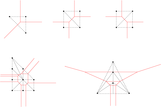
Figure 3: Here we show the graph of the toric diagram in light black and dashes black and the dual graph in solid red. The latter is interpreted as web of $[p,q]$ 5-branes of the type IIB string. The geometries are $\mathbb{C}^{3}$, ${\cal O}(-1)\times{\cal O}(-1)\rightarrow\mathbb{P}^{1}$, with the $\mathbb{P}^{1}$ flopped, ${\cal O}(-K_{P_{\Delta^{(14)}}})\rightarrow{P_{\Delta^{(14)}}}$ , and an $A_{2}$ fibration over $\mathbb{P}^{1}$.

The coordinate ring of $\mathbb{P}_{\Delta_{d}}$ is defined most explicitly in [60] as follows. Let $l(\Delta)$ denote all integer points in $\Delta$ and the vectors $l^{(k)}$, $k=1,\ldots,l(\Delta_{d})-d-1$ specify a basis of linear relations among the points of $\Delta_{d}$, i.e.

$$\sum_{i}l^{(k)}_{i}\nu^{(i)}=0\ .$$ (3.21)

The toric variety can be defined in the coordinate ring $Y_{i}$ as

$$\mathbb{P}_{\Delta}={\mathbb{C}^{|\Sigma(1)|}\setminus Z_{\Delta}\over{\rm Hom}(A_{d-1}(\mathbb{P}_{\Delta}),\mathbb{C}^{*})}\ .$$ (3.22)

Here ${\rm Hom}(A_{d-1}(\mathbb{P}_{\Delta}),\mathbb{C}^{*})=(\mathbb{C}^{*})^{{\rm rank}A_{d-1}(\mathbb{P}_{\Delta})}\times A_{d-1}(\mathbb{P}_{\Delta})_{\rm tors}$ and the $\mathbb{C}^{*}$-action is specified by the $l^{(k)}$ as

$$Y_{i}\mapsto Y_{i}(\mu^{(k)})^{l^{(k)}_{i}}\quad\forall i,$$ (3.23)

with $\mu^{(k)}\in\mathbb{C}^{*}$. $Z_{\Delta}$ is the Stanley-Reisner ideal. Its substraction guarantees well-defined orbits under the torus action. It is determined from a triangulation of $\Delta$ and consists of all loci in the intersection of divisors $D_{i_{1}}\cap\ldots\cap D_{i_{r}}$ for which the set of corresponding points $\{\nu_{i_{1}},\ldots,\nu_{i_{k}}\}$ are not on a common triangle. The triangulation determines also the generators $l^{(k)}$ of the Mori cone, which is dual to the Kähler cone, i.e. to each $l^{(k)}$ there is a dual curve whose volume vanishes at the boundary of the Kähler cone. Since all Mori cones and triangulations have been calculated in [84] we just give an example: Let us label the points of the ${\cal O}(-1)\times{\cal O}(-1)\rightarrow\mathbb{P}^{1}$ polyhedron in figure 3 counter-clockwise starting from the right lower corner, the first triangulation corresponds to a Mori vector $l^{(1)}=(-1,1,-1,1)$. The coordinates $(y_{2}:y_{4})$ are homogeneous coordinates of the compact $\mathbb{P}^{1}$, whose positive volume is the Kähler cone and $y_{2}=y_{4}=0$ is the Stanley-Reisner ideal. $y_{1}$ and $y_{3}$ are the line bundle coordinates. The coordinates of the flopped $\mathbb{P}^{1}$ with $l^{(1)}=(1,-1,1,-1)$ are correspondingly given by $(y_{1}:y_{3})$ etc.

The coordinate ring of $X_{\bar{\Delta}_{d}}$ is defined similarly by (3.22), with $\Delta$ replaced with $\bar{\Delta}$ in the definition of (3.21). Note that the inner point $\bar{\nu}^{(0)}=(1,0,\ldots,0)$ spans now a ray $\Sigma(1)$ and corresponds to a new coordinate belonging to the new non-compact direction of $X_{\bar{\Delta}}$. Note that in this case $\sum_{i}l^{(k)}_{i}=0$, as the points lie in a plane. It is easy to see from (3.23) that this condition ensures the existence of a globally defined $(d+1,0)$-form, hence $X_{nc}=X_{\bar{\Delta}_{d}}$ is a non-compact CY $(d+1)$-fold.

3.5 Global and local mirror symmetry

As it is familiar from Batyrev’s mirror construction [47] we can view each polyhedron $\Delta$ in two ways. Firstly as defining $\mathbb{P}_{\Delta}$ as explained above and secondly as defining the Newton polyhedron for a polynomial $W_{\Delta}(Y)$, where the coordinates of the points determine the exponents of the $Y_{i}$.

It is useful for the following to recall the difference between compact and non-compact toric mirror symmetry. In the compact case the Calabi-Yau $X$, or $X_{\Delta^{*}}$ – the anti-canonical divisor in $\mathbb{P}_{\Delta^{*}}$ – is defined as a section of the anti-canonical bundle

$$W_{\Delta}=\sum_{i=0}^{l(\Delta)-1}a_{i}X_{i}=\sum_{\nu^{(i)}\in\Delta}a_{i}\prod_{\nu^{*(k)}\in\Delta^{*}}Y_{k}^{\langle\nu^{(i)},\nu^{*(k)}\rangle+1}=0$$ (3.24)

in the coordinate ring $Y_{k}$ of $\mathbb{P}_{\Delta^{*}}$. Here the coefficients $a_{i}$ parametrize (redundantly) the complex structure of $X$. In compact mirror symmetry points $\nu^{(i)}$ ($\nu^{*(k)}$) inside codimension one faces of $\Delta$ ($\Delta^{*}$) can be excluded from the sum (products) above, because the corresponding monomials $X_{i}$ can be removed by the automorphism group acting on $\mathbb{P}_{\Delta^{*}}$ while the corresponding variables $Y_{k}$ describe exceptional divisors in the resolution of singularities that vanish outside of $W_{\Delta}=0$.

Similarly the mirror to $X$ called $X^{*}$ (or more specifically $X_{\Delta}$) is defined as a hypersurface

$$W_{\Delta^{*}}=\sum_{i=0}^{l(\Delta^{*})-1}a^{*}_{i}Y_{i}=\sum_{\nu^{*(i)}\in\Delta^{*}}a_{i}^{*}\prod_{\nu^{(k)}\in\Delta}X_{k}^{\langle\nu^{*(i)},\nu^{(k)}\rangle+1}$$ (3.25)

in the coordinate ring of $\mathbb{P}_{\Delta}$.

Note that $\mathbb{P}_{\Delta^{*}}$ can be embedded as a singular variety in $\mathbb{P}^{l(\Delta^{*})}$ with the constraints

$$\prod_{i}Y_{i}^{l^{(k)}_{i}}=1\qquad\forall k\ .$$ (3.26)

By construction the $Y_{i}$ in (3.25) viewed as a function of the $X_{k}$ fulfill this constraint. The quotient construction of mirror symmetry can be realized, if there is an embedding map $\Phi:(\Delta^{*},\Gamma^{*})\rightarrow(\Delta,\Gamma)$. This defines the êtale map from the $X_{i}$ to the $Y_{i}$. For the example of the quintic the relevant charge vector (3.21) is $l^{(1)}=(-5,1,1,1,1,1)$ and the êtale map is

$$\phi:(X_{0}:X_{1}:\ldots:X_{5})\mapsto(\prod_{i=1}^{5}X_{i}:X_{5}^{5}:\ldots:X_{5}^{5})=(Y_{0}:Y_{1}:\ldots:Y_{5})\ ,$$ (3.27)

which is many to one and is made unique by identifying the $X_{k}$ with the mirror quotient group $G$. I.e. ${\rm kern}(\Phi)=G$ and the order of $G$ is the degree of $\Phi$.

For example the pairs $(\Delta_{2},\Delta_{2}^{*})$ define one-dimensional compact Calabi-Yau hypersurfaces $W_{\Delta_{2}}(Y)=0$ in (almost) del Pezzo surfaces $\mathbb{P}_{\Delta^{*}_{2}}$, i.e. elliptic curves and all $a_{i}$ up to one can be set to $0$ or $1$ by the automorphism group of $\mathbb{P}_{\Delta^{*}_{2}}$ and rescalings of $Y_{i}$ leaving (3.26) invariant.

The construction of non-compact mirror symmetry described first in [83] restricts this construction to the coordinate ring defining $X_{nc}$. One starts therefore with

$$W_{\Delta_{d}^{*}}=\sum_{i=0}^{l(\Delta_{d})-1}a^{*}_{i}Y_{i}=0\ ,$$ (3.28)

where $\Delta_{d}^{*}$ is a $d$-dimensional polyhedron, not necessarily reflexive. In the case of a global embedding $X_{nc}\subset X$, $\Delta^{*}_{d}\subset\Delta^{*}_{d^{\prime}\geq d+2}$ is at least a two-codimensional face of a $d^{\prime}$-dimensional reflexive polyhedron $\Delta^{*}_{d^{\prime}}$. In this case $\Delta^{*}_{d}$ defines a ($d$+1)-dimensional lattice $\bar{\Gamma}_{d+1}$ as described at the end of the last section and by the reflexivity of $\Delta^{*}_{d^{\prime}}$ it lies as $\bar{\Delta}^{*}_{d}$ in a hyperplane at distance one from the origin. The corresponding in-complete fan describes the non-compact CY ($d$+1)-fold $X_{\bar{\Delta}_{d}}$ inside the compact CY ($d^{\prime}$-1)-fold. In contrast to the compact mirror symmetry discussed above there are no automorphisms in $X_{\bar{\Delta}_{d}}$ to remove monomials in (3.28), hence the sum runs over all points in $\Delta_{d}$.

Let $l^{(i)}$ generate a basis of linear relations $\sum_{i}l^{(k)}_{k}\bar{\nu}^{(i)}=0$ among the points of $\bar{\Delta}_{n}$, which define (3.26). These relations restrict the possibility to undo deformations of the $a_{i}^{*}$ by rescalings of $Y_{i}$, leaving $l(\Delta^{*}_{d})-d-1$ independent deformations of the B-model. A convenient way to introduce these in the curve is to set all $a^{*}_{i}=1$ and modify (3.26) to

$$\prod_{i}Y_{i}^{l^{(k)}_{i}}=z_{k}\qquad\forall k\ .$$ (3.29)

Here we use Batyrev’s coordinates

$$z_{k}=\prod_{i}{a^{*}}_{i}^{l^{(k)}_{i}}$$ (3.30)

so that $z_{k}=0$ is the large complex structure point.

In this description (3.28) with $a^{*}_{i}=1$, (3.29) and a $\mathbb{C}^{*}$-identification $Y_{i}\sim\mu Y_{i}$ with $\mu\in\mathbb{C}^{*}$ define the mirror geometry. It can be written as a $(d-1)$-dimensional affine variety by adding to the singularity $W_{\Delta^{*}}=0$ trivial non-compact normal directions as quadratic coordinates. E.g. for $\Delta^{*}_{2}$ it is

$$H(X,Y,{\underline{z}}):=W_{\Delta^{*}_{2}}(X,Y,{\underline{z}})=uv\ .$$ (3.31)

Note that in order to solve (3.29) in favor of two variables say $X,Y$ we have to view $Y_{i}$ as $\mathbb{C}^{*}$-variables. $W_{\Delta^{*}}(X,Y)=0$ becomes in general a Laurant polynomial in $\mathbb{C}^{*}$-variables defining a genus $g$ Riemann surface $\Sigma$ with $h$ punctures. Here $g$ is the number of inner points in $\Delta^{*}_{2}$ and $h=l(\Delta^{*}_{2})-g$. The nowhere vanishing holomorphic $(3,0)$-form can be defined in a coordinate patch of the $(d+1)$-dimensional ambient space by a contour integral

$$\Omega=\frac{a_{0}}{(2\pi i)}\oint_{W=0}\left(\prod_{p}Y_{p}\right)\frac{\wedge_{j=1}^{d+1}\frac{dY_{j}}{Y_{j}}}{W}$$ (3.32)

and restricts to the Riemann-surface $H(X,Y,{\underline{z}})$ as [13]

$$\lambda=\log(X)\frac{dY}{Y}\ .$$ (3.33)

In local mirror symmetry we study the variation of mixed Hodge structures of the non-compact local Calabi-Yau spaces using this logarithmic form on $H(X,Y,{\underline{z}})$ in particular by analysing its Picard-Fuchs equation.

The formalism was certainly well known in the study of mixed Hodge structure assocuated to singularties, see e.g. [26] or [109] for a review. The variation of the mixed Hodge structure for log Calabi-Yau spaces $(X,D)$ with $D$ a divisor in particular the isomorphism

$$\phi:H^{3}(X\setminus D)\rightarrow\bigoplus_{p+q=3}H^{q}(X,\Omega^{p}_{\bar{X}}(\log(D))$$ (3.34)

to the log cohomology has been used to calculate superpotentials in [63] and a recent application to stable degenerations [97] is similar to the local mirror symmetry for vertical divisors with a transition to del Pezzo surfaces discussed in section 3.6.2.

The inner points deform the complex structure of $\Sigma$, while the punctures define by the counting of independent deformations $l(\Delta)-g-3$ independent residue values of $\lambda$ refered to as masses $m_{i}$ and $i=1,\ldots,l(\Delta)-g-3$.

In the case of a del Pezzo basis there is only one inner point whose coefficient $a_{0}$ is identified with the complex structure of the elliptic curve $W_{\Delta}^{*}(X,Y)=0$, physically related to the gauge coupling of the $U(1)$ theory on the Coulomb branch while $l(\Delta^{*}_{2})-4$ of the $a^{*}_{i}$ are identified with mass parameters.

There is a physical interpretation for the dual graph associated to a general triangulated polyhedron. It can be viewed as a web of $[p,q]$5-branes for the type IIB string. These 5-branes fill the $0,\ldots,5$ directions of the five-dimensional space-time. The figure corresponds to the $(5,6)$-plane, where the 5-branes extend as lines, whose slope is given by the $SL(2,\mathbb{Z})$ charge $[p,q]$.

3.6 Global embeddings of the local geometries

Let us now discuss two kinds of global embeddings of local geometries in compact Calabi-Yau spaces $X$. Both are related to elliptic fibrations. In the first the del Pezzo appears as the base and all $(1,1)$-classes of the del Pezzo are are $(1,1)$-classes in $X$ in the second a rational elliptic fibration typically a half K3 appears as a so-called vertical divisor over blow-ups in the base. After flopping out a number of $\mathbb{P}^{1}$ the rational elliptic fibration becomes a del Pezzo, which can be blown down.

Both global embeddings can be studied in very concrete global embeddings of the reflexive polyhedra $(\Delta^{B}_{n},\Delta^{B*}_{n})$ into a pair of reflexive polyhedra $(\Delta_{n+2},\Delta^{*}_{n+2})$, so that the anti-canonical hypersurface in $\mathbb{P}_{\Delta^{*}_{n+1}}$ gives rise to an elliptically fibred Calabi-Yau $(n+1)$-fold over the toric base $\mathbb{P}_{\Delta_{n}^{B*}}$ with an interesting structure of global sections.

For notational simplicity and because the virtual dimension of the moduli space of stable pairs is only zero for threefolds, we outline the embedding of two-dimensional polyhedra in a four-dimensional polyhedron, which gives rise to an elliptically fibred threefold over a toric del Pezzo base $\mathbb{P}_{\Delta_{2}^{B*}}$, specified by $\Delta_{2}^{B*}\in\Delta_{4}^{*}$. However everything in this section, except for (3.38), generalized trivially to arbitrary dimension.

The reflexive pair $(\Delta^{*}_{4},\Delta_{4})$ is the convex hull of the following points

$$\footnotesize\begin{array}[]{|ccc|ccc|}\lx@intercol\hfil\nu^{*}_{i}\in\Delta_{4}^{*}\hfil\lx@intercol&\lx@intercol\hfil\nu_{j}\in\Delta_{4}\hfil\lx@intercol\\ &&\nu_{i}^{F*}&&\nu_{j}^{F}&\\ &\Delta^{B*}_{2}&\vdots&s_{ij}\Delta^{B}_{2}&\vdots&\\ &&\nu_{i}^{F*}&&\nu_{j}^{F}&\\ &0\ldots 0&&0\dots 0&&\\ &\vdots&\Delta^{*F}_{2}&\vdots&\Delta^{F}_{2}&\\ &0\ldots 0&&0\ldots 0&&\\ \end{array}\,.$$ (3.35)

Here we consider all points $\nu_{j}^{F*}\in\Delta_{F}^{*}$ and define

$$s_{ij}=\langle\nu_{i}^{F},\nu_{j}^{F*}\rangle+1\in\mathbb{N}\ .$$ (3.36)

Note that we scaled $\Delta^{B}_{2}\rightarrow s_{ij}\Delta_{2}^{B}$. This means to scale the coordinates of the points of $\Delta^{B}_{2}$ by $s_{ij}$ while keeping the original lattice basis, i.e. $s_{ij}\Delta_{2}^{B}$, contains in general more lattice points. Note that the vertices of $\Delta^{*}$ ($\Delta$) are given by the vertices of the polyhedra $\Delta^{*F}_{2}$ ($\Delta_{2}^{*F})$ and $\Delta^{*B}_{2}$ ($s_{ij}\Delta_{2}^{B}$) respectively.

Both polyhedra $\Delta$ and $\Delta^{*}$ have the following features in common, which we spell out only for $\Delta$ in this paragraph, where we also call $s_{ij}\Delta_{2}^{B}$ simply $\Delta_{2}^{B}$. They contain a polyhedron $\Delta_{2}^{F}\subset\Delta_{4}$ that is a sub-polyhedron of $\Delta_{4}$ and shares the unique inner point. It also implies an exact sequence of the lattices $0\rightarrow\Gamma_{F}\rightarrow\Gamma\rightarrow\Gamma_{B}\rightarrow 0$, where $\Gamma_{F}$ is the sublattice associated to $\Delta_{2}^{F}$. Further the base polyhedron $\Delta_{2}^{B}$ is a two-face of $\Delta_{4}$ and the image of a projection along the fibre polyhedron, i.e. obtained by identifying all other points modulo $\Delta_{2}^{F}$. These are necessary conditions for $P_{{\Delta_{4}}}$ to have a fibration

$$\mathbb{P}_{{\Delta_{4}}}\rightarrow\mathbb{P}_{\Delta_{2}^{B}}$$ (3.37)

over $P_{\Delta_{2}^{B}}$ with $P_{\Delta_{2}^{F}}$ as the generic fibre. As stated in [67] a sufficient condition (F1) for the existence of the above fibration as a (smooth) and flat one, is the existence of a fan $\Sigma_{\Delta}$ (whose cones have lattice volume one) and which is defined by a triangulation of $\Delta$ that lifts from a fan $\Sigma_{\Delta^{B}_{2}}$. The hypersurface $W_{\Delta_{4}*}=0$ in $P_{{\Delta_{4}}}$ becomes then an elliptic fibration whose generic fibre is defined as the section of the anti-canonical bundle in $P_{\Delta_{2}^{F}}$.

It easy to see that (F1) is fulfilled for $P_{{\Delta^{*}_{4}}}$ so that $X$ given by $W_{\Delta_{4}}=0$ is a smooth and flat elliptic fibration. The problem in establishing (F1) for $X^{*}$ is the scaling of $\Delta_{2}^{B}$. In this case $W_{\Delta^{*}_{4}}=0$ is in general only a non-flat elliptic fibration.

The Euler number and the Hodge number of $X$ depend in a simple way on the base and the type of the fibration as

$$\chi(X)=-a_{F}\int_{B}c_{1}^{2},\qquad h_{11}(X)=l(\Delta^{*}_{B})-4+b_{F}+t_{F}\ .$$ (3.38)

where $a_{F},b_{F},T_{F}$ depend only on the fibre type, which is in turn specifed by $\Delta^{*F}$ and $\nu^{*F}$. We therefore give $a_{F}/b_{F}(t_{F})$ at the inequivalent corners of the polyhedra in figure 1. The contribution of the base classes to $h_{11}(X)$ is $l(\Delta^{*}_{B})-3$. They correspond to vertical divisors. These are rational surfaces. One of the $b_{F}+t_{F}+1$ classes comes from the zero-section of the base in the fibre or if $t_{f}>0$ this can be a $t_{f}+1$ multi-section. The rest can come either from additional rational sections or from gauge symmetry enhancements. Since the Euler number is proportional to $c_{1}^{2}$ the gauge symmetry enhancement occurs along a multiple of the canonical divisor. Which of these possibilities is realized can be distinguished by analyzing which Kodaira fibre occur in $W_{\Delta_{4}}=0$, we will discuss this further for some specific fibrations below.

3.6.1 The del Pezzo surface as base

Let us take the tenth polyhedron $\Delta(10)$ as $\Delta_{2}^{*F}$ i.e. $\Delta_{2}^{*F}=\text{conv}\{(1,0)$, $(-1,2)$, $(-1,-1)\}$ and for $\nu_{3}^{F*}=(-1,-2)$. Since $\Delta_{2}^{*F}$ is self-dual, $\Delta_{2}^{F}=\text{conv}\{(1,0)$, $(-1,2)$, $(-1,-1)\}$ and $\nu_{j}^{F}=(-1,-2)$, so $s_{ij}=6$. Start for the base with the first polyhedron, i.e. $\Delta_{2}^{*B}=\Delta(1)$. In a hopefully obvious notation referring to figure 1 we denote this manifold $X_{(\Delta^{F}(10)\times_{F}^{3}\Delta^{B}(1))}$. Since $\mathbb{P}_{\Delta(1)}=\mathbb{P}^{2}$, this yields an elliptic fibration over $\mathbb{P}^{2}$. On the corresponding corner we find $a_{F}=60$ and $b_{F}=2$, i.e. we get $\chi(X)=-60\times 9=-540$, $h_{11}(X)=2$ and this is an elliptic fibration with a single section, since there are no additional ‘twisted‘ states, if we chose $\Delta_{2}^{*B}=\Delta(3)$, we obtain an elliptic fibration with a single section over the blow-up of $\mathbb{P}^{2}$ the Hirzebruch surface $\mathbb{F}_{1}$ with $\chi(X)=-60\times 8=-480$ and $h_{11}(X)=4$ etc. This creates a first series of 15 fibrations with one section. Denoting the coordinates associated to the points $CO=\{(0,0,0,0)$, $(0,0,1,0)$, $(0,0,-1,-1)$, $(0,0,-1,2)\}$ by $x_{0}$, $y$, $x$ and $z$ we see from (3.24) that $W_{\Delta}$ is in the Tate form

$$x_{0}W_{\Delta}=x_{0}(y^{2}+h_{1}({\underline{Y}}_{B})xyz+h_{3}({\underline{Y}}_{B})yz^{3}-(x^{3}+h_{2}({\underline{Y}}_{B})x^{2}z^{2}+h_{6}({\underline{Y}}_{B})z^{6}))$$ (3.39)

and the pure monomials in the variables ${\underline{Y}}_{B}$ corresponding to the coordinate ring of the base are multiplied with $z$. Hence at $z=0$ we get a section, which is the un-constrained Fano variety $\mathbb{P}_{\Sigma_{\Delta^{B*}}}$. The constraint $W_{\Delta}=0$ is solved by $x^{3}=y^{2}$, which has a unique solution, up to automorphisms in chosen $P_{\Delta}^{*F}$, so that this fibration has a single section. I.e. we get a fibration map

$$X_{\Delta}\rightarrow\mathbb{P}_{{\Delta^{*B}_{2}}}\,,$$ (3.40)

whose generic fibre is the elliptic curve ${\cal E}=X_{\Delta_{2}^{*F}}$. The non-compact Calabi-Yau manifold ${\cal O}(-K_{P_{{\Delta^{B*}_{2}}}})\rightarrow{P_{{\Delta^{B*}_{2}}}}$ is obtained by scaling the volume of the ${\cal E}$ fibre to infinity. This limit can be made very precise, because the Mori vector, that corresponds to the fibre is given by $l^{(E)}=(-6,3,2,1,0,\ldots,0)$, w.r.t. the points in $CO$ and has no entry at other points. By (3.30) $z_{E}\sim e^{-t_{E}}$ where $t_{E}$ is the volume of the fibre, so the limit is $z_{E}=0$. We discuss the local mirror further in section 3.7.

3.6.2 The del Pezzo as a transition of a vertical divisor and rational sections

If one blows up a $\mathbb{P}^{1}$ in the base one gets as additional divisor a vertical divisor [45, 6], which is a half $K3$ realized as a rational elliptic fibration ${\cal E}\rightarrow\mathbb{P}^{1}$ over the exceptional $\mathbb{P}^{1}$. It inherits the fibration structure of the generic fibre, e.g. the number of rational or multi-sections, which makes general fibrations ${\cal E}=X_{\Delta_{2}^{*F}}$ interesting to study.

We give an example below, but discuss first the most generic case ${\cal E}=X_{\Delta(10)}$. The simplest case is when we blow up the $\mathbb{P}^{2}$ and obtain a Hirzebruch surface $\mathbb{F}_{1}$. With the choice of the Mori cone

$$l^{({\cal E})}=(-6;3,2,1,0,0,0,0),\quad l^{(\mathbb{F}_{1}^{F})}=(0;0,0,-1,-1,1,1,0),\quad l^{(\mathbb{F}_{1}^{B})}=(0;0,0,-2,1,0,0,1)\ ,$$ (3.41)

$X$ has an elliptic as well as a K3 fibration, where $l^{({\cal E})}$ corresponds to the elliptic fibre, $l^{(\mathbb{F}_{1}^{B})}$ represents the base of the K3 fibration and the base of $\mathbb{F}_{1}$, while $l^{(\mathbb{F}_{1}^{F})}$ corresponds to the exceptional $\mathbb{P}^{1}$, the fibre of the Hirzebruch surface, and the base of the elliptic surface. As explained in section 3.1, if we flop this $\mathbb{P}^{1}$ then the elliptic surface ${\cal E}\rightarrow\mathbb{P}^{1}$ becomes the elliptic pencil (3.11) with exactly one base base point i.e. the $E_{8}$ del Pezzo. As explained in [45, 6] the new phase is characterized by $l^{(1)}=l^{({\cal E})}+l^{(\mathbb{F}_{1}^{F})}=(-6;3,2,0,-1,1,1,0)$ and representing the canonical class in the del Pezzo, $l^{(2)}=-l^{(\mathbb{F}_{1}^{F})}$ representing the flopped curve and $l^{(2)}=l^{(\mathbb{F}_{1}^{F})}+l^{(\mathbb{F}_{1}^{B})}$ representing the hyperplane class in $\mathbb{P}^{2}$. Now if a del Pezzo shrinks the Higgs branch of the corresponding $N=2$ field theory opens up and by deforming the singularity one gets, according to (3.38) with $a_{F}=60$, a transition to a Calabi-Yau manifold $X^{\prime}$ with $h_{21}(X^{\prime})=h_{21}(X)+29$, $h_{11}(X^{\prime})=h_{11}(X)-1$, i.e. since one vector multiplet is going to be massive by the Higgs effect, the Higgs branch is of dimension $a_{F}/2$. The fibres

$${\cal E}=X_{\Delta(10)},\ \ X_{\Delta(4)},\ \ X_{\Delta(1)}$$ (3.42)

correspond to the $E_{8}$, $E_{7}$ and $E_{6}$ fibres. In general the dimension of the Higgs branch is $a_{F}/2=30,\ 18$ and $12$ appearing at one corner of these polyhedra is the dual Coxeter number of the group. These models have one, two and three multi-sections, i.e. if we blow down the base of the elliptic surface as before, we get elliptic pencils with one, two and three base points, corresponding to the $E_{8}$, $E_{7}$ and $E_{6}$ del Pezzo surfaces.

In the case of vertical divisors not all classes of rational surfaces are classes in the Calabi-Yau space $X$, i.e. the image of the inclusion map $i^{*}:H^{1,1}(X)\rightarrow H^{1,1}(S)$ has rank $1\leq k\leq h^{1,1}(S)$. According to the theorem of Néron, sections of the elliptic surface are in the image and as already observed in [45] they can be extended as sections over the entire base. Once they are flopped the elliptic pencil develops base points and the corresponding del Pezzo can be shrunken. This was studied in [6] for $E_{7}$ and $E_{6}$ with toric divisors and as a an explicetly mentioned by-product fibrations with a holomorphic zero-section and additional rational toric sections were constructed and their Kähler classes identified as Wilson line parameters that break the $E_{8}$ of the tensionless string sucessively to $E_{7}$ and $E_{6}$. These Kähler parameters correspond to the new rational global sections. Moreover the precise breaking of the $E_{8}$ representations into $U(1)\times E_{7}$ and further into $U(1)_{1}\times U(1)_{2}\times E_{6}$ representations was studied on the level of genus zero BPS states [6]. The $U(1)$’s are supported at the new global sections. The $U(1)_{1}\times U(1)_{2}\times E_{6}$ model is based $\Delta^{*F}_{2}=\Delta(5)$ the double blow-up of $\mathbb{P}^{2}$ with $\nu_{2}^{F*}=\nu_{2}(\Delta(5))$. Then $a_{F}/b_{f}(t_{f})=24/4(0)$ and if we fibre over $\mathbb{P}^{2}_{\Delta(3)}=\mathbb{F}_{1}$ the $\chi=-192$, $h_{11}=5$ manifold $X_{(\Delta^{F}(5)\times_{F}^{2}\Delta^{B}(3))}$ allows for an $E_{6}$ del Pezzo transition to $X_{(\Delta^{F}(5)\times_{F}^{2}\Delta^{B}(1))}$ the elliptic fibration over $\mathbb{P}^{2}$ with $\chi=-216$, $h_{11}=4$. Since the discussion of the toric realization of the transition with more sections in [6] was too sketchy we give the Mori cone data in the appendix.

These examples have been re-discovered and interesting variants that have three rational sections have been discussed in detail in  [55, 56]. The dual $\Delta^{F}_{2}$ has the Newton polynom (A.1) with $s_{4}=s_{10}=0$. This curve has therefore three sections at $[x:y:z]=\{[0:0:1],[0:1:0],[0:s_{9}:-s_{7}]\}$, where in $X$ $s_{7}$ and $s_{9}$ are line bundles over the base. Calling the associated divisors $S_{7}$ and $S_{9}$ a straightforward application of the adjunction formula [56] yields $\chi(X)=\int_{B}(-24c_{1}^{2}+8c_{1}S_{7}-4S_{7}^{2}+8c_{1}S_{9}+2S_{7}S_{9}-4S_{9}^{2})$, i.e. the four cases $S_{7}=S_{9}=0$, $S_{7}=c_{1},S_{9}=0$, $S_{7}=0,S_{9}=c_{1}$ and $S_{7}=S_{9}=c_{1}$ in which $\chi(X)$ becomes proportional to $c_{1}^{2}$ reproduce the $X$ with the Euler numbers that are realized toric hypersurfaces given by the combination of the data in Fig 1 with (3.35).

A more extrem case is to choose $\Delta_{2}^{*B}=\Delta_{2}^{*F}=\Delta(15)$ and $\nu_{i}^{F*}=(0,0)$. Then $\nu_{i}^{F}=(0,0)$ and we get $\chi(X)=-6\times 3=-18$ and $h_{11}(X)=10-4+8=14$. It is also easy to see that in these cases, where we fibre using the anti-canonical class $\nu_{i}^{F*}=(0,0)$, we have $s_{ij}=1$ and $X^{*}$ is also a flat elliptic fibration with the dual fibre polyhedron. In fact both $X$ and $X^{*}$ exhibit two elliptic fibrations with base and fibre polyhedron exchanged. Using the formula for intersections for the second elliptic fibration one discovers in this case an $SU(3)^{3}$ gauge enhancement over the anti-canonical divisor over the base.

3.7 A short cut to the mirror geometry

The mirror of the del Pezzo in the base must occur as a specialization of the constraint (3.25). Due to the form of $\Delta$ we can always find a triangulation that leads to an elliptic fibration, not necessarily a smooth and flat one. However for the discussion of the complex deformations of the mirror geometry, this is good enough. Denoting the coordinates associated to $(0,0,-1,-1),\,(0,0,2,-1)\,\text{and}\,(0,0,-1,1)$ again by $y$, $x$ and $z$, $W_{\Delta*}$ is realized in the Tate form. In the mirror geometry the restriction is given by $y=x=0$ implying $z\neq 0$ because of the form of the Stanley-Reisner ideal and hence the constraint

$$W_{\Delta^{*}}=z^{6}h^{6}_{\Delta^{*}_{B}}({\underline{X}}^{\prime}_{B})=0\$$ (3.43)

implies $h^{6}_{\Delta^{*}_{B}}({\underline{X}}^{\prime}_{B})=0$. Further note the possibility of rescaling $z$ which leads to the afore mentioned $\mathbb{C}^{*}$-identification $X_{iB}^{\prime}\sim\mu X_{Bi}^{\prime}$ with $\mu\in\mathbb{C}^{*}$. Secondly the scaling (3.36) is only due to the global embedding and the corresponding refinement of the lattice of $\Delta^{\prime}$ w.r.t to $\Delta$ can be undone in the local case by an êtale map

$$\phi_{s_{ij}}:(X_{0}^{\prime},\ldots:X_{l(\Delta_{B})}^{\prime})\mapsto(X_{0}^{s_{ij}}:\ldots:X_{l(\Delta_{B})}^{s_{ij}})\ .$$ (3.44)

Hence the mirror geometry to ${\cal O}(-K_{\mathbb{P}_{\Delta^{*}}})\rightarrow K_{\mathbb{P}_{\Delta}^{*}})$ is simply given as the Newton polynomial

$$H({\underline{X}})=h^{6}_{\Delta^{*}_{B}}({\underline{X}}_{B})=0$$ (3.45)

of $\Delta^{*B}_{2}$ itself.

We define therefore the coordinates of Newton polynomials of $\Delta^{*B}$ for the biggest three polyhedra in which all other polyhedra are embeddable. These numbres of polyhedra are $16$ yielding the most general cubic in $\mathbb{P}^{2}$, $13$ for the most general quartic in $(\mathbb{P}(1,1,2)$ and $15$ for the most general bi-quadratic in $\mathbb{P}^{1}\times\mathbb{P}^{1}$. The Newton polynom is defined by (3.25) letting $\nu^{*(i)}$ run over $\Delta_{2}^{B*}$ and $\nu^{*(i)}$ over the corners of the dual polyhedron $\Delta_{2}^{B}$ and the coordinate ring is subject to (3.44). This yields the coordinates as indicated in figure 4.

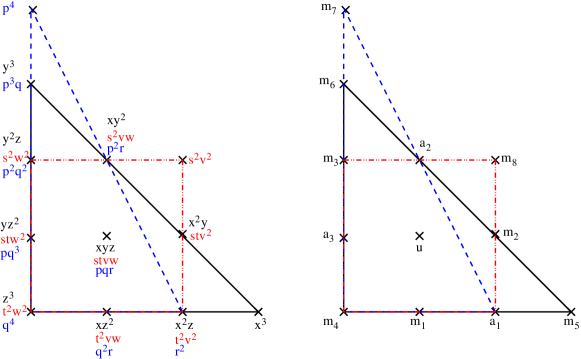
Figure 4: All 16 reflexive polyhedra can be embedded into this diagram.

Using the remaining scaling of the above projective spaces we can write

$$H(X,Y,{\underline{a^{*}}})=h^{6}_{\Delta^{*}_{B}}(X,Y,{\underline{a^{*}}})$$ (3.46)

as an inhomogeous equation. Note that there as many independent $a^{*}_{i}$ as there are relations between the points on $\Delta^{*B}$. So in two dimensions we can gauge away three $a_{i}^{*}$. The formalism does not depend on the existence of a global embedding and in particular $\Delta^{*B}$ must not be reflexive. However for reflexive polyhedra the corresponding elliptic curves can be readily brought into Weierstrass form using simple transformation algorithms such as Nagell’s algorithm, which is very useful for further calculations and will be summarized in Appendix A. Moreover the Mori cones and triangulations have been calculated. These data will be used to relate the parameters $a_{i}^{*}$ in the Newton polynomials to the Kähler parameters. The upshot is that the compact part, i.e. the elliptic curve, of the mirror to the local del Pezzo geometry is the anti-canonical class in the del Pezzo surface defined by the Newton polynomial of $\Delta_{B}^{*}$ which fixes a choice of the automorphism group.

It follows from the above and the general discussion at the end of section 3.5 that the mirror curves to toric del Pezzo surfaces have one complex structure parameter called $u$ and $l(\Delta)-4$ mass parameters called $m_{i}$, corresponding to the canonical class of del Pezzo and the $e_{i}$-curves respectively. If more then three points are blown up, the del Pezzo surfaces have in addition to the Kähler structure moduli, complex structure moduli and the toric description by the reflexive polyhedra with $l(\Delta)-4>3$ holds only at a special fixed value of the complex structure. This is not a problem for the goal to describe the full Kähler structure moduli space of the del Pezzo surface by the elliptic curve as long as $h_{1,1}(S)\leq 7$ (the bound comes simply from polyhedron 16 which has the maximal $l(\Delta)=10$), because Kähler and complex structure moduli decouple in $N=2$ theories. Above $h_{1,1}(S)>7$ i.e. for the $E_{8}$ and $E_{7}$ del Pezzo we find torically no mirror in which all masses can be turned on.

However we can construct the full anti-canonical model $(S,{\cal E})$ for the $E_{8}$ and $E_{7}$ del Pezzo by completing the Weyl orbits for the mass parameters in polyhedron 10 and 14. We note that by the construction in section 3.2 and 3.3 the description of the mirror of the del Pezzo and the description of the gauge bundle over ${\cal E}$ are on the same moduli space. In particular within the half $K3$ the moduli of the Kodaira singularities, i.e. $[p,q]$ 7-branes positions and the heretoric bundle moduli are unified in one moduli space.

4 Physical interpretations

The physical aspects of the refined BPS states on local del Pezzo surfaces were reviewed in [2] from the point of view of five-dimensional $N=1$ gauge theory compatified on $\mathbb{S}^{1}_{5}\times\mathbb{R}^{4}$, but our ability to explore here the full moduli space of an elliptically fibred $\frac{1}{2}K3$ locally in an elliptically fibred Calabi-Yau manifold makes them in fact central in the following string/M-/F-theory dualities.

4.1 Small instanton and E-string perspective

In this section we will argue that the refined stable pair invariants count the higher spin partition function of the tensionless string that is the F-theory dual to a small $E_{8}$ instanton on the heterotic side.

To cancel the anomaly in the heterotic string on $K3$ one has to have $\sum_{a}c_{2}(V_{a})=c_{2}(T_{K3})$ and in particular the total instanton number of the vector bundle(s) $V_{a}$ has to be $24$. Due to the absence of vector multiplet moduli, the dynamics of the six-dimensional $N=1$ field theory with eight supercharges in two left spinors $(2,0)$ is described by the Higgs effect. It was first argued [10] that when one of these $SO(32)$ instanton shrinks to zero size, i.e. its curvature is concentrated in a point on the K3, space-time develops an infinite tube in which an unbounded increasing dilaton profile develops, a $SP(1)$ gauge group is enhanced and hypermultiplets in the $({\bf 32},{\bf 2})$ become massless. A single shrinking instanton corresponds to the nucleation of a solitonic heterotic five-brane that scales with ${1\over g_{s}}$ exactly as the Dirichlet-brane in the Type I theory, with which it can be identified under heterotic-Type I duality. The phenomenon is independent of the heterotic string coupling outside the tube. In accordance with the unoriented type I open string sector the maximal non-perturbative gauge symmetry enhancement in the heterotic $SO(32)$ string, when all instantons shrink at one point is $Sp(24)$.

However the shrinking of instantons in $E_{8}\times E_{8}$ heterotic string cannot be described by the Higgs dynamics, because the dimensions of the $E_{8}$ representation are too big relative to the dimension of the moduli space of a single $E_{8}$ instanton which is $29$. It has therefore been suggested that the dynamical effect is due to a tensionless string. This string is similar in nature as the self-dual string of type IIB on K3 from a D3-brane wrapping a holomorphic curve, that becomes tensionsless when the latter shrinks.

Upon compactification on a circle $\mathbb{S}^{1}_{5}$ one can use T-duality on this circle between heterotic $SO(32)$ and $E_{8}\times E_{8}$ to relate the small instanton dynamics in five dimensions [11]. Massless new states have to appear in five dimensions, which confirms the picture of a tensionless string. The strong coupling of the $E_{8}\times E_{8}$ string theory is conjectured to be M-theory on an interval $S_{11}^{1}/\mathbb{Z}_{2}$ and the solitonic heterotic five-brane is identified with the M5-brane. Purely based on the ten-dimensional anomaly cancellation mechanism in was argued in [57] purely that on the two fix points there are a novel kind of 9-branes with an $E_{8}$ super Yang-Mills theory on each of them. Since the dilaton profile grows near the gauge bundle singularity, the dynamical effect related to the shrinking in one $E_{8}$ instanton occurs for any value of the asymptotic heterotic string coupling and can been interpreted in the strong coupling description as the nucleation of a M5-brane close to one $E_{8}$-branes. M2-branes can end on the M5-branes [51] and it has been argued that they can end on the $E_{8}$-branes [11], yielding the tensionless string.

The analysis of the spectrum of this six-dimensional tensionsless string has been iniated in [12, 6]. In [6] it starts with analyzing the BPS states encoded in (8.5), which describes winding one $n_{b}=1$ in the base of the $\frac{1}{2}K3$ discussed at the beginning of section (3.6.2). Here the image of $i^{*}$ has rank two: The class of the section of the base $\mathbb{P}^{1}$ and the class of the fibre and the modularity of this expression is due to (3.15).

Using the hypothesis that the right-movers of the tensionsless string are as the ones for the M-string or Green-Schwarz string in six dimensions that couples to the six-dimensional tensor $N=2$ tensor multiplet that arises from two parallel M5-branes, i.e. using an ${\cal O}(4)$ lightcone quantization one gets from the $252$ unrefined BPS genus zero states at winding $d_{f}=1$ the space-time spectrum [6]

$$\left[{\bf 248};4(0,0)\oplus\left(\frac{1}{2},0\right)\oplus\left(0,\frac{1}{2}\right)\right]+\left[{\bf 1};4\left(\frac{1}{2},\frac{1}{2}\right)\oplus\left(1,\frac{1}{2}\right)\oplus\left(\frac{1}{2},1\right)\oplus\left(0,\frac{1}{2}\right)\oplus\left(\frac{1}{2},0\right)\right]\ .$$ (4.1)

Here the left representations refer to the $E_{8}$ representations and the right ones to the space-time representations in six dimensions. As has been argued using the M/F-theory duality in [6], all diagonal states $(d_{b},d_{f})=(n,n)$ become part of the massless spectrum of the tensionless string at the transition point, where the volume of the curve $t_{E}+t_{\mathbb{F}^{F}_{1}}$ specified by (3.41) becomes zero. As explained below (3.41) this requires that the $\mathbb{F}^{F}_{1}$ is flopped so that its volume formally becomes negative. The first $n=1,2,3,4,\ldots$ diagonal unrefined BPS states are at genus zero $n^{(0)}_{n}=252,-9252,848628,-114265008,\ldots$ at genus one $n^{(1)}_{n}=-2,760,-246790,76413833,\ldots$ at genus two $n^{(1)}_{n}=0,-4,30464,-26631112,\ldots$ etc. Clearly they can hardly be interpreted in themselves as individual BPS states of the tensionless string. First of all, since they are not positive, they can be at most an index, secondly they do not fall in any obvious way into representations of $E_{8}$ or the space-time spin.

These problems all evaporate if we consider the refined stable pair invariants, as decribed in section 5.1. First of all they are all positive, secondly they do fall in a simple way in $E_{8}$ representations and finally they do reproduce the only individual BPS states that could be inferred in [6], namely the one above (4.1) from the splitting of the $E_{8}$ representation into the five-dimensional spins $(j_{L},j_{R})$

$$\left[{\bf 248};(0,0)\right]+\left[{\bf 1};\left(\frac{1}{2},\frac{1}{2}\right)\right]\ .$$ (4.2)

We conclude that the refined stable pair invariants do count the full tower of massless BPS states including all spins! With the hypothesis above the six-dimensional space-time representations can be reconstructed at all levels $n$. Of course in this application we directly count stable pair invariants in the positive Kähler cone of the local del Pezzo and argue that they become all massless if the latter shrinks to zero size. It is very suggestive but not entirely clear that these states are stable bound states in this limit. Of course our formalism allows to calculate the $F^{(n,g)}$ at any place in the Kähler moduli space of the geometry. In particular as we argue in section 5.1 that the spectrum at the conifold, where the volume vanishes is identical to the large volume point due to the self-duality of the $E_{8}$ lattice. This underlines the claim that we found the stable spectrum of the tensionless string. So it is a quite concrete proposal for the spectrum for a conformal higher spin theory of the type recently analyzed in [58, 59].

As proposed in [6] we can turn on Wilson lines parametrized by vectors ${\bf W}_{\alpha}$ in the Cartan algebra of $E_{8}$. In our local description of the $E_{n}$ curves mirror to $E_{n}$ del Pezzo surfaces this literally means to shift the masses $m_{i}$. To be concrete we have to choose a basis of the wheight lattice to parametrize the characters by $m_{i}$ in the same basis and call $\Lambda$ the charge of a BPS state. Then the shift of the masses by the Wilson lines is simply given by

$${\bf m}\rightarrow{\bf m}+\sum_{\alpha}{\bf\Lambda}\cdot W_{\alpha}\ .$$ (4.3)

This will in general break $E_{8}$ in $U(1)^{k}\times E_{8-k}$, where the $U(1)^{k}$ can be globalized in F-theory as discussed in section (3.6.2).

4.2 The $[p,q]$-string perspective

F-theory describes the varying axion-dilaton background $\tau=C_{0}+ie^{-\phi}$ of type IIB compactifications on manifolds $B_{d}$ with positive canonical class by the complex structure $\tau$ of an elliptic fibration ${\cal E}\rightarrow B_{d}$, so that the total space is a Calabi-Yau manifold $Y_{d+1}$. The latter condition requires the fibre to degenerate over divisors $d_{i}\in B_{d}$ so that the canonical class fulfills

$$K_{B_{d}}=\sum_{i}a_{i}d_{i},$$ (4.4)

where $a_{i}$ are rational numbers associated to the possible Kodaira types of the singular fibres, which are elliptic singularities whose Hirzebruch-Jung sphere configurations intersect in an affine $ADE$ Dynkin diagram, the simplest one, called $I_{0}$, beeing just a nodal curve for which $a=\frac{1}{12}$ making $Y_{2}=K3$ over $B_{1}=\mathbb{P}^{1}$ with $24$ $I_{0}$ fibres at points $u_{i}\in\mathbb{P}^{1}$, $i=1,\ldots,24$ the simplest example. The single vanishing cycle $\gamma=$$\left[\begin{array}[]{c}p\\ q\end{array}\right]$$\in H_{1}({\cal E},\mathbb{Z})$ at say $u_{1}\in\mathbb{P}^{1}$ ($d_{1}\in B_{d}$) determines the $[p,q]$-charge of the 7-branes that extend over $d_{1}$ and the non-compact directions. The Picard-Lefshetz monodromy action on $H_{1}({\cal E},\mathbb{Z})$ along a counter-clockwise loop encircling $u_{1}$ is like in the rank one Seiberg-Witten families over $z$ given by [54]

$$M_{p,q}=\left(\begin{array}[]{cc}1-pq&p^{2}\\ -q^{2}&1+pq\end{array}\right)\ .$$ (4.5)

It acts as subgroup of the ${\rm SL}(2,\mathbb{Z})$-symmetry of type II on the doublet $(H_{3},F_{3})$ of the NS and RR three-forms and their sources: the fundamental $\left[\begin{array}[]{c}p\\ q\end{array}\right]$=$\left[\begin{array}[]{c}1\\ 0\end{array}\right]$- and $D$ $\left[\begin{array}[]{c}p\\ q\end{array}\right]$=$\left[\begin{array}[]{c}0\\ 1\end{array}\right]$- string and as ${\rm PSL}(2,\mathbb{Z})$-transformation on $\tau$. This happens at a cut emanating from the $[p,q]$ 7-brane position, whose precise position must be irrelevant for physical questions, in particular regarding BPS states from string junctions.

The global monodromy is encoded in the Weierstrass form of the family as in (2.11), where we view $u$ as parameter on the base while $\vec{m}$ parametrizes the position of the 7-branes, and is not trivial. As a consequence there are mutually non-local $[p,q]$ 7-branes and no global perturbative description of F-theory, not even an understanding of the full spectrum of its BPS states in space-time, like the one we inferred for the tensionless string in the last section. What comes closest to it is to consider groups of in general non-local $[p,q]$ 7-branes and construct BPS states such that the gauge bosons that correspond to the roots are given by string junctions. The simplest group of such branes is the configuration of Sen in which he sets $g_{2}=cf^{2}$ and $g_{3}=f^{3}$ with $f=\prod_{i=1}^{4}(u-u^{0}_{i})$, so that $j$ and hence $\tau$ become constant. The monodromy at each $u=u^{0}_{i}$ $i=1,\ldots,4$ is $M=-{\bf 1}$, so the configuration has no net charge and since $M$ is the involution on ${\cal E}$ the configuration at this point must be four 7-branes of charge $[1,0]$ and an O7-brane, with charge $[-4,0]$, the latter splits into a $[-2,-2]$ and $[-2,2]$. Of course the orientifold brane configuration gives a $SO(8)$ gauge symmetry, the breaking of which is described by moving the 7-branes away from $u^{0}_{i}$. Moreover since $g_{2}\sim u^{2}$, $g_{3}\sim u^{3}$ and the gauge symmetry acts as flavour symmetry on the $m_{i}$ the problem of constructing the local deformation of the brane configuration is the same as constructing the $SU(2)$, $N_{f}=4$ Seiberg-Witten curve. Physically this can be argued more intuitively in the D3-probe-brane picture in which always the gauge and flavour symmetry are exchanged.

The general approach to construct the non-Cartan gauge bosons, which in particular extends to the $E_{n}$ groups, is by string junctions. For them one has the follwing key properties

• J.1 String junctions are configurations of ${\footnotesize{\left[\begin{array}[]{c}p\\ q\end{array}\right]}}_{i}$-strings $i=1,\ldots,N$, which meet in a single point, subject to a non-force condition

  $$\sum_{i=1}^{N}\left[\begin{array}[]{c}p\\ q\end{array}\right]_{i}=0\,.$$ (4.6)

• J.2 Two ${\footnotesize{\left[\begin{array}[]{c}p\\ q\end{array}\right]}}$-strings can end on each other iff they are compatible

  $$\left[\begin{array}[]{c}p\\ q\end{array}\right]_{i}\wedge\left[\begin{array}[]{c}p\\ q\end{array}\right]_{k}=p_{i}q_{k}-q_{i}p_{k}=\pm 1\ ,$$ (4.7)

  the sign depending on the orientation of the corresponding cycle in $H_{1}({\cal E},\mathbb{Z})$. 3-junctions are BPS configurations iff (4.7) holds for each pair [106].

• J.3 Each ${\footnotesize{\left[\begin{array}[]{c}p\\ q\end{array}\right]}}$-string line emerging from the junction can end on a $[p,q]$ 7-brane, where $\gamma={\footnotesize{\left[\begin{array}[]{c}p\\ q\end{array}\right]}}\in H_{1}({\cal E},\mathbb{Z})$ shrinks.

The general idea is that the string junctions extend the fundamental $\left[\begin{array}[]{c}1\\ 0\end{array}\right]$ open strings that lead to the $A_{n}$ gauge symmetry on stacks of $n+1$ fundamental branes to stacks of non-mutual $[p,q]$ 7-branes connected by string junctions. $N=3$ turns out to be enough to get all roots of the exceptional groups [34].

The most relevant questions are what are the low energy states of these configurations, what is their moduli space, how to quantize them, i.e. what are the associated BPS states. Unfortunately the anwers are to a large extent unknown. It is known of course that in the presence of a 7-brane a configuration, with a given asymptotic charge at the ends, is independent of the position of the $[p,q]$ 7-brane cut, i.e. (4.5, 4.6, 4.7) are compatible, as explained e.g in [34] and shown in figure [57].

Figure 5: If a $[r,s]^{t}$ string is moved over the $[p,q]$ 7-brane leaving its cut and if $[p,q]^{t}$ is compatible with $[r,s]^{t}$ then a $[p,q]^{t}$-string, connecting $[p,q]$ with $[r,s]^{t}$ and forming there a junction, is created.

This fact as well as J.1-J.3 makes it possible to lift topological configurations of string junctions ending on $[p,q]$ 7-branes to closed curves in the total space of a two complex dimensional ${\cal E}$ fibration and search for their minimal energy configuration [107]. It is claimed [107] that the polarisation can be can be chosen, so that the geodesic minimality in the $u$ plane is equivalent to the lifted curve being holomorphic in the complex structure. Moreover the natural intersection on junctions defined on junctions [107, 37] should yield the intersection on holomorphic curves, which gives simple constraints on certain BPS junctions [107]. The metric for the geodesic minimality is the same then the one used in [108] only that there the lift is supposed to yield special Lagrangian 3-cycles.

So in order to search for the BPS states in our geometries we might attempt to identify stable pairs in the rational elliptic surface, whose pure sheaf of complex dimension one is supported on a holomorphic curve ${\rm ch}_{2}({\cal F})=\beta$ in a mixed class of fibre and base of the massless $\frac{1}{2}K3$.

These classes precisely decompose into Weyl orbits by formula (9) and the list of results for the diagonal classes in the section below is quite encouraging. The numbers with the lowest degree and spin yields for the $E_{8}$ case the $8+240$ in the trivial and the first non-trivial Weyl orbit, i.e. the $E_{8}$ gauge bosons for which the $\left[\begin{array}[]{c}p\\ q\end{array}\right]$-string junctions were designed for. Moreover it is well-known in the heterotic/type II duality, most noticable in the YZ formula [110], that the BPS states of those string oscillation encoded the elliptic genus are mapped to $\chi({\cal F})=n$ i.e. the “$D0$ brane” content of the stable pair, which yields the spin content of the refined stable pair invariant. Indeed in the simplest case, as in [110], they are counted by the Göttsche formula for Hilbert schemes of points on the symmetric product, a structure that is refined for the $n_{b}=1$ classes in the $\frac{1}{2}K3$ in section 8.2. This makes it reasonable to assume that the exitation of $\left[\begin{array}[]{c}p\\ q\end{array}\right]$-strings are encoded in the $(j_{L},j_{R})$ spin content. Beside the issue of stability, which we do not address here, it should be clear that due the flavor symmetries the $\mathbb{C}^{*}$-action used in the Bialynicki-Birula decomposition there can be shifts in the association of mass and spin, e.g. the diagonal Kähler class could be shifted as $t\rightarrow t-a+c(\epsilon_{1}+\epsilon_{2})$. The mirror construction relates the position of the $[p,q]$ 7-branes in the curve (2.11) and turning them on splits the representrations of the $E_{8}$ into massive ones and massless ones associated the unbroken subgroups. All this seems sufficient evidence to conclude that refined BPS-states do capture properties of the infinite towers of BPS states associated to the $\left[\begin{array}[]{c}p\\ q\end{array}\right]$-strings suspended between mutual non-local $[p,q]$ 7-branes.

5 The $D_{5},E_{6},E_{7}$ and $E_{8}$ del Pezzo surfaces

The formalism described in section 2.3, the description of mirror symmetry of local del Pezzo surfaces in section 3.7 together with the general Weierstrass form given in section A allows to recursively calculate the amplitudes $F^{(n,g)}$. Then the formulae (2.8) and (2.9) can be used to extract the invariants $N_{j_{L},j_{R}}^{\beta}$. As a warm-up we consider special one parameter del Pezzo’s of the type indicated above. In this one parameter family one sums over all classes $\Lambda^{\prime}$ of the del Pezzo surface, by setting the corresponding Kähler classes to $t_{i}\rightarrow 0$, i.e. $q_{i}=e^{t_{i}}=1$. Since the Weyl group of the corresponding Lie algebra acts on $\Lambda^{\prime}$ we expect to find the states organized in the dimensions of the Weyl orbits. Physically the specialization corresponds to setting the mass parameters in the five-dimensional theory to zero. We will denote $\beta\in H_{2}(M,\mathbb{Z})$ simply by the positive integer $d$, the degree of the holomorphic maps.

5.1 The $E_{8}$ del Pezzo surface

According to section 3.7 the massless $E_{8}$ can be obtained from the polyhedron 10 with all mass parameters on the edges set to zero. This is simply done by setting in (A.1) (see table) all parameters to zero except $m_{2}=m_{4}=m_{6}=1$ while keeping $\tilde{u}$. The right large complex structure variable $u=\frac{1}{\tilde{u}^{\frac{1}{6}}}$ is found based on the analysis of the Mori cone below (6.70). Then we get after a rescaling $g_{i}\rightarrow\lambda^{i}g_{i}$ with $\lambda=18u^{7/3}$

$$g_{2}=27u^{4},\qquad g_{3}=-27u^{6}(1-864u)\ .$$ (5.1)

so that near $u=0$, we get $\frac{dt}{du}=\frac{1}{u}+60+13860u+4084080u^{2}+{\cal O}(u^{3})$. The $j$-function

$$j=\frac{1}{1728u(1-432u)}\ .$$ (5.2)

identifies this as the special family whose monodromy group is classic and has already been discussed in [89]. As a consistency check we can also take the curve (B.1) and turn off all the Wilson lines by setting the $\chi_{i}(0)$ to the values of the dimensions of the weight moduls. Let us define the Dynkin diagram of the affine $E_{8}$ as

where we denote by the bold numbers the Coxeter labels. The smaller numbers give simply an ordering of the basis of Cartan generators and the basis for the weights. Let us denote by $w_{i}$ the weight of the classical Lie algebra with a $1$ at the $i$th entry and $w_{0}$ the trivial weight. We record the dimensions of the corresponding weight modules

$$\begin{array}[]{rl}\chi_{1}(0)&=3875,\quad\chi_{2}(0)=147250,\quad\chi_{3}(0)=6696000,\quad\chi_{4}(0)=6899079264,\\ \chi_{5}(0)&=146325270,\quad\chi_{6}(0)=2450240,\quad\chi_{7}(0)=30380,\quad\chi_{8}(0)=248\ .\end{array}$$ (5.3)

Specializing (B.1) gives indeed the same family as can be seen by comparing the $j$-functions.

For the BPS states $N^{d}_{j_{L},J_{R}}$ at $d=1$ one gets:

$2j_{L}\backslash 2j_{R}$	0	1
0	248
1		1

$d=1$

It is obvious that the adjoint represention $248$ of $E_{8}$ appears as the spin $N_{0,0}^{1}$, which decomposes into two Weyl orbits with the weights $w_{1}+8w_{0}$. I. e. we are counting exactly the BPS numbers of the $[p,q]$-string configurations, which are relevant for the gauge theory enhancement in F-theory. Note that the contributions of different Weyl orbits come in general from curves with different genus. In this way also the higher spin invariants fall systematically into Weyl orbits of weights of $E_{8}$. E.g. $3876=1+3875$, where the latter decomposes in the Weyl orbits of $w_{1}+7w_{8}+35w_{0}$. The multiplicities of the Weyl Orbits are encoded in the solution of the $\frac{1}{2}K3$ model by the formula (9.21), where we report the dimension of some lower $E_{8}$ Weyl orbits in equation (9).

$2j_{L}\backslash 2j_{R}$	0	1	2	3
0		3876
1			248
2				1

$d=2$

At $d=3$ we see the decompositions into representaions $4124=1+248+3875$, $34504=1+248+30380$, $34504=1+248+30380$, $151374=1+248+3875+147250$ and $30628=248+30380$

$2j_{L}\backslash 2j_{R}$	0	1	2	3	4	5	6
0	30628		151374		248
1		4124		34504		1
2	1		248		4124
3				1		248
4							1

$d=3$

while for higher degree the geometric multiplicities of the Weyl orbits become bigger with the lower spins farer away from the maximal spin, still it obvious how the states decompose into Weyl orbits, e.g.

$2j_{L}\backslash 2j_{R}$	0	1	2	3	4	5	6	7	8	9	10
0		3480992		7726504		212879		248
1	185878		1209127		3632614		38876		1
2		38876		251755		1030753		4373
3	248		4373		39125		217003		249
4		1		249		4373		35000		1
5					1		249		4125
6								1		248
7											1

$d=4$

$7726504=2+9\times 248+6\times 3875+6\times 147250+669600$.

5.2 The $E_{7}$ del Pezzo surface

The massless $E_{7}$ del Pezzo corresponds to the polyhedron 13 with all parameters on the edges set to zero. Again this is simply done by specializing the Weierstrass form (A.2) to

$$a_{1}=1,\quad m_{4}=1,\quad m_{5}=1,\quad u=\frac{1}{(-\tilde{u})^{\frac{1}{4}}}\$$ (5.4)

while setting all other parameters to zero. Again the inverse quartic root identification of $u=\frac{1}{(-\tilde{u})^{\frac{1}{4}}}$ can be predicted from the Mori cone vector $l=(-4,1,1,2)$. It could be also obtained by firstly requiring at large radius $t(u)\sim\log(u)$ and at the conifold $t_{D}(u)\sim\Delta$. This also fixes the $-1$ in (5.4), in fact that $t(u)=\log(u)-12u+210u^{2}+{\cal O}(u^{3})$ and secondly knowing that genus zero curves exist at $d=1$.

Relative to (5.4) we have to scale the $g_{2}$ and $g_{3}$ by $\lambda=18iu^{\frac{2}{5}}$ yielding

$$g^{b}_{2}=27u^{4}(1-192u),\quad g_{3}^{b}=27u^{6}(1+576u)\$$ (5.5)

and the $j$-function as

$$j_{b}=\frac{(192u-1)^{3}}{1728u(64u+1)^{2}}\ .$$ (5.6)

It is well-known that massless theories can be formulated on isogenous curves [54]. These curves are not distinguished by their Picard-Fuchs equation, neither for the holomorphic nor the meromophic differential, but they are distinguished by a choice of a relative factor $\kappa\in\mathbb{N}_{+}$ in the normalization of the $a$- and the $b$-cycles. As pointed out in [54] this exchanges the two cusp points – corresponding to the large radius and conifold points – of the curves, but is not a symmetry of the $N=2$ theory neither of the topological string. In the context of the del Pezzo surfaces the existence of isogeneous curves has been discussed in [85]. It finds a natural interpretation in terms of the center of $E_{n}$ given in (3.9) as follows. Since the Picard-Fuchs equations depend only on the linear relations among the points in the polyhedra, the polyhedron 4 with one mass at the edge of the corner set to zero will lead to the same Picard-Fuchs operator. Now with the Weierstrass form obtained by embedding polyhedron 4 into polyhedron 13 by setting all coefficients to zero exept

$$a_{1}=1,\quad a_{2}=1,\quad m_{5}=1,\quad u=\frac{1}{(\tilde{u})^{\frac{1}{4}}}\,,$$ (5.7)

we can precisely understand the relation between the two geometries. With $\lambda=18u^{\frac{2}{5}}$ we get now

$$g^{s}_{2}=27u^{4}(48u+1),\quad g_{3}^{s}=27u^{6}(72u+1)\$$ (5.8)

and the $j$-function as

$$j_{s}=\frac{(48u+1)^{3}}{1728u^{2}(64u+1)}\$$ (5.9)

so that the $\mathbb{Z}_{2}$ transformations

$$\mathbb{Z}_{2}:u\mapsto-\frac{1}{64}-u,\quad\mathbb{Z}_{2}:j_{b}\leftrightarrow j_{s},\quad\mathbb{Z}_{2}:\tau_{s}\leftrightarrow 2\tau_{b}$$ (5.10)

exchanges as in [54] the conifold with the large radius point and identifies $j_{b}\leftrightarrow j_{s}$ and rescales the $U(1)$-coupling. However to get integral charges for the matter representations, or equivalently integral Kähler classes, one has to choose the curve corresponding to the big polyhedron. Note that the last relation in (5.10) can be already seen from the fact that $\Delta=1+64u$ appears quadratically in the denominator of $j_{b}$. The story is analogous for the $E_{6}$ group with the big polyhedron being polyhedron 15 and the small polyhedron being polyhedron 1. So we conclude that the volumes of polyhedra $P_{b}$ and $P_{s}$ the are related to the center of the groups, or the volumes of the fundamental cell in the lattices $\Lambda^{\prime}$ and $\Lambda^{\prime\prime}$ as

$$\frac{{\rm Vol}(P_{b})}{{\rm Vol}(P_{s})}=\frac{{\rm Vol}(\Lambda^{\prime\prime})}{{\rm Vol}(\Lambda^{\prime})}$$ (5.11)

and the existence of the self-dual polyhedron 10 is a consequence of the self-duality of the $E_{8}$ lattice. We further notice that the $j$-function of the massless $E_{7}$ curve of B.1

$$j_{E7}^{es}=\frac{(u_{es}-36)^{3}}{(1728(u_{es}-52)}$$ (5.12)

is not very naturally related to $j_{b}(u_{b})$ or $j_{s}(u_{s})$

$$u_{es}=-12-\frac{1}{u_{s}},\quad u_{es}=\frac{52-768u_{b}}{1+64u_{b}}\ .$$ (5.13)

Let us agree on the Dynkin diagram of $E_{7}$ in the following conventions

$$\begin{array}[]{rl}&\chi_{1}(0)=133,\quad\chi_{2}(0)=912,\quad\chi_{3}(0)=8645,\quad\chi_{4}(0)=365750,\quad\chi_{5}(0)=27664,\\ &\chi_{6}(0)=1539,\quad\chi_{7}(0)=56\ .\end{array}$$ (5.14)

From either the big or the small polyhedron we get the following refined BPS invariants. Again there are the Weyl orbits for curves in different genera which to combine in simple representations of $E_{7}$.

$2j_{L}\backslash 2j_{R}$	0
0	56
$d$=1

$2j_{L}\backslash 2j_{R}$	0	1	2
0		133
1			1
$d$=2

$2j_{L}\backslash 2j_{R}$	0	1	2	3
0	56		912
1				56
$d$=3

We note that there is a periodicity with the degree mod 2 in the contributions of the BPS states with highest spins. In even degree we always find for the highest spin the trivial and the adjoint representation $133$ in the Weyl orbits $w_{1}+7w_{0}$ of $E_{7}$, while in odd degrees we find the $56$ representation in a single Weyl orbit. This is a consequence of the nontrivial center of $E_{7}$ (3.9), which is reflected on the square root of the line bundle ${\cal Q}$ for the $E_{7}$ case.

At $d=3$ the $912$, $w_{2}+6w_{7}$ representation appears and again we find the behaviour that the higher degree stable pair invariants decompose in a simple fashion into representations and hence Weyl orbits. The systematic can again be understood form the solution of the $\frac{1}{2}K3$ and formula (9.21). The relevant dimensions of the Weyl orbit for the $E_{5}=D_{5},\ldots,E_{7}$ goups are summarized in table 6.

E.g. at $d=4$: $8778=8645+133$, with $8645$ decomposes as $w_{3}+5w_{6}+22w_{1}+77w_{0}$ and $1673=1539+133+1$ with $1539=w_{6}+6w_{1}+27w_{0}$.

$2j_{L}\backslash 2j_{R}$	0	1	2	3	4	5	6
0		1673		8778		1
1			134		1673
2				1		133
3							1

$d=4$

At degree $d=4$ we have the following decomposition $1024=912+2\times 56$, $7504=4\times 1539+912+2\times 133+3\times 56+2$, $8472=5\times 1539+5\times 133+2\times 56$, $36080=27664+5\times 1539+5\times 133+56$ and $93688=3\times 27664+8645+1539+3\times 133+2\times 56+1$.

$2j_{L}\backslash 2j_{R}$	0	1	2	3	4	5	6	7	8
0	6592		36080		93688		968
1		968		8472		36080		56
2			56		1024		7504
3						56		968
4									56

$d=5$

$2j_{L}\backslash 2j_{R}$	0	1	2	3	4	5	6	7	8	9	10	11	12
0		225912		650050		1062065		54419		133
1	10451		73839		289109		650184		13588		1
2		1807		13855		75512		234691		1807
3	1		134		1808		13855		61924		134
4				1		134		1808		12048		1
5							1		134		1674
6										1		133
7													1

$d=6$

5.3 The $E_{6}$ del Pezzo surface

As we mentioned before, we specialize the polyhedron 15 to the massless case by setting all coefficients in (A.8) to zero except of

$$m_{4}=1,\quad m_{5}=1,\quad m_{6}=1,\quad u=\frac{1}{\tilde{u}^{1/3}}\ .$$ (5.15)

With $\lambda=18u^{\frac{8}{3}}$ we get

$$g_{2}=27u^{4}(1-216u),\quad g_{3}=27u^{6}(1+540u-5832u^{2})\$$ (5.16)

hence the $j$-function of the $\Gamma_{0}(3)$ curve.

$$j_{b}=-\frac{(1-216u)^{3}}{1728u(1+27u)^{3}}\ .$$ (5.17)

Similar the isogeneous $\Gamma(3)$ curve is obtained by considering the small polyhedron 1 by setting $a_{2}=1$, $m_{2}=1$, $m_{4}=1$ and $u=\frac{1}{\tilde{u}^{1/3}}$, which yields with the same scaling $\lambda$, $g_{2}=27u^{4}(24u+1)$ and $g_{3}=27u^{6}\left(216u^{2}+36u+1\right)$ so

$$j_{s}=-\frac{(1+24u)^{3}}{1728u^{3}(1+27u)}\$$ (5.18)

and the relating data between the isogeneous curves are

$$\mathbb{Z}_{2}:u\mapsto-\frac{1}{27}-u,\quad\mathbb{Z}_{2}:j_{b}\leftrightarrow j_{s},\quad\mathbb{Z}_{2}:\tau_{s}\leftrightarrow 3\tau_{b}\,.$$ (5.19)

Note that the massless $E_{6}$ curve of B.1

$$j_{E6}^{es}=\frac{(u_{es}-18)^{3}(u_{es}+6)}{1728(u_{es}-21)}$$ (5.20)

is again not completely naturally related to $j_{b/s}(u_{b/s})$

$$u_{es}=-6-\frac{1}{u_{s}},\quad u_{es}=\frac{21-162u_{b}}{1+2bu_{b}}\ .$$ (5.21)

We record the characters according to the above basis of weights

$$\chi_{1}(0)=27,\quad\chi_{2}(0)=78,\quad\chi_{3}(0)=351,\quad\chi_{4}(0)=2925,\quad\chi_{5}(0)=351,\quad\chi_{6}(0)=27\ .$$ (5.22)

The low degree spin invariants fall in these representations.

$2j_{L}\backslash 2j_{R}$	0
0	27
$d$=1

$2j_{L}\backslash 2j_{R}$	0	1
0		27
$d$=2

$2j_{L}\backslash 2j_{R}$	0	1	2	3
0	1		78
1				1
$d$=3

$2j_{L}\backslash 2j_{R}$	0	1	2	3	4
0		27		351
1					27
$d$=4

Note that the periodicity in which the adjoint representation appears is now the degree $d$ modulo 3 as expected from the center of $E_{6}$.

The first splitting representation that appears is the $378=351+27$ where $351$ splits in the Weyl orbits $w_{3}+5w_{6}$ and further $1755=5\times 351$, see (9.21) and table 6.

$2j_{L}\backslash 2j_{R}$	0	1	2	3	4	5	6
0	27		378		1755
1				27		378
2							27

$d=5$

$2j_{L}\backslash 2j_{R}$	0	1	2	3	4	5	6	7	8	9
0		730		3732		8984		78
1			79		808		3732		1
2				1		79		730
3							1		78
4										1

$d=6$

$2j_{L}\backslash 2j_{R}$	0	1	2	3	4	5	6	7	8	9	10	11
0	2133		10584		30240		47439		2133
1		378		2889		12717		30240		405
2			27		405		2889		10584		27
3						27		405		2484
4									27		378
5												27

$d=7$

5.4 The $D_{5}$ del Pezzo surface

Finally we discuss the case of the $D_{5}$ surface which can be obtained from the polyhedra 2 (small) and 15 (big). We consider again the massless limit by the following choice of coefficients and redefinition of $u$

$$a_{1}=i,\quad m_{3}=i,\quad m_{4}=i,\quad m_{8}=i,\quad u=\tilde{u}^{-\frac{1}{2}}\quad(\text{big}){}$$

$$a_{2}=i,\quad a_{3}=i,\quad m_{1}=i,\quad m_{2}=i,\quad u=\tilde{u}^{-\frac{1}{2}}\quad(\text{small}).$$ (5.23)

All the other mass parameters vanish. Accordingly, one obtains the respective Weierstrass normal forms

$$g_{2} = 27u^{4}\left(256u^{2}+16u+1\right),{}$$

$$g_{3} = -27u^{6}\left(4096u^{3}+384u^{2}-24u-1\right),\quad\text{big polyhedron},$$ (5.24)

$$g_{2} = 27\left(\frac{1}{u^{2}}+\frac{16}{u}+16\right)u^{6},{}$$

$$g_{3} = 27\left(\frac{1}{u^{3}}+\frac{24}{u^{2}}+\frac{120}{u}-64\right)u^{9},\quad\text{small polyhedron}.$$ (5.25)

In both cases we have performed a recaling with

$$\lambda=18u^{3}$$ (5.26)

in order to arrive at the respective expressions for $g_{2}$ and $g_{3}$. Finally the $j$-functions are given as

$$j_{b}=\frac{\left(256u^{2}+16u+1\right)^{3}}{1728u^{2}(16u+1)^{2}},\qquad j_{s}=\frac{\left(16u^{2}+16u+1\right)^{3}}{1728u^{4}(16u+1)}.$$ (5.27)

In contrast to the previous cases ($E_{6},E_{7},E_{8}$) we observe a different behaviour concerning the exchange of conifold locus and large radius point

$$\mathbb{Z}_{2}:u\mapsto-u-\frac{1}{16},\quad\mathbb{Z}_{2}:j_{b}\leftrightarrow j_{b},\quad j_{s}\leftrightarrow j^{\prime}_{s}=-\frac{\left(256u^{2}-224u+1\right)^{3}}{1728u(16u+1)^{4}},\quad\mathbb{Z}_{2}:\tau_{s}\leftrightarrow 4\tau_{s}^{\prime}.$$ (5.28)

Instead the $j$-functions of the two polyhedra are related by the map

$$u_{b}\mapsto-\frac{16u-(8u+1)\sqrt{16u+1}+1}{32(16u+1)}.$$ (5.29)

We end the discussion by comparing the curves to the massless $D5$ curve given by Sakai and Eguchi. This is given by setting again the characters to the dimensions of the fundamental representations in (B.8). The Weierstrass data of this curve are given by

$$g_{2}=\frac{1}{12}(u+4)^{2}\left(u^{2}-8u-32\right),\qquad g_{3}=\frac{1}{216}(u+4)^{3}\left(u^{3}-12u^{2}-24u+224\right),$$ (5.30)

and the $j$-function reads

$$j^{es}=\frac{\left(32u_{es}^{2}+8u_{es}-1\right)^{3}}{1728u_{es}^{4}\left(48u_{es}^{2}+8u_{es}-1\right)}$$ (5.31)

In contrast to the previous cases, this curve is not connected to any of the two previous curves by a birational coordinate transformation.

The Dynkin diagram of $\hat{D}_{5}$

leads to the following dimensions of the weight moduls

$$\chi_{1}(0)=10,\quad\chi_{2}(0)=45,\quad\chi_{3}(0)=120,\quad\chi_{4}(0)=16,\quad\chi_{5}(0)=16\ .$$ (5.32)

We see the periodicity with respect to the degree is now modulo four and the adjoint representation of $D5$ appears for the first time at $d=4$. The representation $45$ falls in the Weyl orbits $w_{2}+5w_{0}$. The Weyl orbit of $w_{2}$ is $40$-dimensional and gets contributions only from genus zero curves, while the $w_{i}$ get contributions from a genus two curve, whose leading contribution is at spin $[1/2,2]$.

$2j_{L}\backslash 2j_{R}$	0
0	16
$d$=1

$2j_{L}\backslash 2j_{R}$	0	1
0		10
$d$=2

$2j_{L}\backslash 2j_{R}$	0	1	2
0			16
$d$=3

$2j_{L}\backslash 2j_{R}$	0	1	2	3	4
0		1		45
1					1
$d$=4

$2j_{L}\backslash 2j_{R}$	0	1	2	3	4	5
0			16		144
1						16

$d=5$

$2j_{L}\backslash 2j_{R}$	0	1	2	3	4	5	6	7
0		10		130		456
1					10		130
2								10

$d=6$

$2j_{L}\backslash 2j_{R}$	0	1	2	3	4	5	6	7	8	9
0	16		160		736		1440		16
1				16		176		736
2							16		160
3										16

$d=7$

$2j_{L}\backslash 2j_{R}$	0	1	2	3	4	5	6	7	8	9	10	11	12
0		311		1345		3431		4726		257
1			46		357		1602		3431		46
2				1		46		357		1345		1
3							1		46		311
4										1		45
5													1

$d=8$

5.5 An alternative approach to the massless cases

Alternatively we use the Picard-Fuchs equations, the Yukawa couplings, i.e. the usual B-model methods, that also apply in the compact cases. The complex geometry of the mirror manifolds are described by the Picard-Fuchs differential equations

$$(\theta_{z}^{2}+c_{0}z\prod_{i=1}^{2}(\theta_{z}+1-a_{i}))\theta_{z}\int_{\gamma_{i}}\Omega=0,$$ (5.33)

where $z$ is the complex structure modulus in the mirror manifold and $\theta_{z}=z\partial_{z}$. $a_{1},a_{2}$ and $c_{0}$ are classical constants of the the Calabi-Yau manifolds. $c_{0}$ is a normalization constant for the complex structure parameter $z$ such that $t=\log(z)+\mathcal{O}(z)$ around $z\sim 0$ corresponds to the Kähler modulus in the large volume limit. The vectors $\vec{a}=(a_{1},a_{2})$ satisfy $a_{1}+a_{2}=1$ and are given as follows for various one-parameter families of Calabi-Yau manifolds we consider

$$\mathbb{P}^{2}:~{}\vec{a}=(\frac{1}{3},\frac{2}{3}),~{}~{}~{}~{}\mathbb{P}^{1}\times\mathbb{P}^{1}:~{}\vec{a}=(\frac{1}{2},\frac{1}{2}),~{}~{}~{}~{}D_{5}:~{}\vec{a}=(\frac{1}{2},\frac{1}{2}),~{}~{}~{}~{}$$

$$E_{6}:~{}\vec{a}=(\frac{1}{3},\frac{2}{3}),~{}~{}~{}~{}E_{7}:~{}\vec{a}=(\frac{1}{4},\frac{3}{4}),~{}~{}~{}~{}~{}~{}~{}~{}~{}E_{8}:~{}\vec{a}=(\frac{1}{6},\frac{5}{6}).$$ (5.34)

The $E_{n}$ ($n=5,6,7,8$) del Pezzo surfaces can be represented as complete intersections of degree $(2,2)$ in $\mathbb{P}^{4}$, a degree 3 hypersurface in $\mathbb{P}^{3}$, a degree 4 hypersurface in weighted projective space $\mathbb{P}^{3}(1,1,1,2)$ and a degree six hypersurface in $P^{3}(1,1,2,3)$. In these cases the normalization constant $c_{0}$ can be computed as $c_{0}=(\prod_{i}d_{i}^{d_{i}})/(\prod_{j}w_{j}^{w_{j}})$ where $d_{i}$ are the degree(s) of hypersurfaces or complete intersections, and $w_{j}$ are weights of the ambient projective space. The constant is $c_{0}=27$ for the $\mathbb{P}^{2}$ model and $c_{0}=-16$ for the $\mathbb{P}^{1}\times\mathbb{P}^{1}$ model.

The prepotential $F^{(0,0)}(t)$ is determined by the Picard-Fuchs (PF) equation (5.33) from the fact that the mirror map $t(z)$ and derivative $\partial_{t}F^{(0,0)}(t)$ are solutions to the PF equation besides the constant solution. The normalization of the prepotential is fixed by the classical intersection number $\kappa$ as $F^{(0,0)}(t)=-\frac{\kappa}{6}t^{3}+\cdots$. The intersection number can be calculated by the formula $\kappa=(\prod_{i}d_{i})/(\prod_{j}w_{j})$ in the $E_{n}$ models. The numbers are $\kappa=\frac{1}{3}$ for the $\mathbb{P}^{2}$ model and $\kappa=1$ for the $\mathbb{P}^{1}\times\mathbb{P}^{1}$ model. We list the constants $c_{0}$ and $\kappa$ for the Calabi-Yau models in Table 1.

CY	$\mathbb{P}^{2}$	$\mathbb{P}^{1}\times\mathbb{P}^{1}$	$D_{5}$	$E_{6}$	$E_{7}$	$E_{8}$
$c_{0}$	27	-16	16	27	64	432
$\kappa$	$\frac{1}{3}$	1	4	3	2	1

Table 1: The constants $c_{0}$ and $\kappa$ for the Calabi-Yau models.

We discuss next the genus one amplitudes $F^{(1,0)}$ and $F^{(0,1)}$. The $F^{(1,0)}$ amplitude is holomorphic while the amplitude $F^{(0,1)}$ has a holomorphic anomaly which is determined by the genus one holomorphic anomaly equation [49]. Both amplitudes have logarithmic cuts for the discriminant $\Delta(z)=1+c_{0}z$ whose coefficients are determined by the genus one gap boundary conditions at the conifold point $\Delta(z)=0$. Furthermore, it turns out that the amplitudes also contain a logarithmic piece $\log(z)$. We can write the amplitudes as

$$F^{(1,0)} = \frac{\log(\Delta(z))-c^{(1,0)}\log(z)}{24},$$

$$F^{(0,1)} = -\frac{1}{2}\log(\partial_{z}t(z))-\frac{1}{12}(\log(\Delta(z))+c^{(0,1)}\log(z)),$$ (5.35)

where we use the constants $c^{(1,0)}$ and $c^{(0,1)}$ to denote the coefficients for $\log(z)$ terms in the refined amplitudes. We determine the constants for the Calabi-Yau models and list them in Table 2.

CY	$\mathbb{P}^{2}$	$\mathbb{P}^{1}\times\mathbb{P}^{1}$	$D_{5}$	$E_{6}$	$E_{7}$	$E_{8}$
$c^{(1,0)}$	1	2	8	9	10	11
$c^{(0,1)}$	7	7	4	3	2	1

Table 2: The constants $c^{(1,0)}$ and $c^{(0,1)}$ for the Calabi-Yau models.

The three-point Yukawa coupling and the Kähler metric in the moduli space are given up to an anti-holomorphic factor by

$$C_{zzz}=-\frac{\kappa}{z^{3}(1+c_{0}z)},~{}~{}~{}G_{z\bar{z}}\sim\partial_{z}t\,.$$ (5.36)

The Christoffel connection in the holomorphic limit $\Gamma_{zz}^{z}=\partial_{t}z(\partial^{2}_{z}t)$ is not a rational function of $z$. There is a relation with the propagator which satisfies ${\partial}_{\bar{z}}S^{zz}=\bar{C}_{\bar{z}}^{zz}$,

$$\Gamma_{zz}^{z}=-C_{zzz}S^{zz}+f_{z}$$ (5.37)

where $f_{z}$ is a rational function of $z$ since the anti-holomorphic derivatives $\bar{\partial}_{\bar{z}}$ of both sides are the same. For the one-parameter models we simply denote the propagator as $S\equiv S^{zz}$. The rational function $f_{z}$ is a holomorphic ambiguity that we can choose such that the propagator $S$ has a nice behavior near the special singular points in the moduli space

$$f_{z}=-\frac{6a_{1}+5}{6z}-\frac{c_{0}}{6(1+c_{0}z)}$$ (5.38)

where $a_{1}$ is the constant in (5.5) and $c_{0}$ is the normalization constant in table 1. With this choice of ambiguity $f_{z}$, the propagator $S$ is regular at the conifold point $z=-\frac{1}{c_{0}}$. Near the orbifold point $z^{-1}\sim 0$, the propagator generically scales as $S\sim z^{3}$ and we have chosen the constant $(6a_{1}+5)$ in $f_{z}$ to cancel the leading $z^{3}$ term so that the scaling behavior is less singular near the orbifold point as $S\sim z^{2}$. The cancellation can be seen by noting that the flat coordinate scales as $t\sim z^{-a_{1}}$ near the orbifold point $z^{-1}\sim 0$, and accordingly the Christoffel connection scales as $\Gamma_{zz}^{z}\sim-(a_{1}+1)z^{-1}$ and cancels the leading term in $f_{z}$.

The derivative of the propagator can be derived from the special geometry relation,

$$D_{z}S=-C_{zzz}S^{2}+\tilde{f}(z),$$ (5.39)

where the covariant derivative reads $D_{z}S=(\partial_{z}+2\Gamma_{zz}^{z})S$. The holomorphic ambiguity $\tilde{f}(z)$ is a rational function with a simple pole at $\Delta(z)$, and it can be fixed by computing $S$ and $\Gamma_{zz}^{z}$ in the holomorphic limit.

The propagator $S$ is the only an-holomorphic component in the higher genus amplitudes, and the generalized holomorphic anomaly for the refined theory is

$$\partial_{S}F^{(n,g)}(S,z)=\frac{1}{2}[D_{z}^{2}F^{(n,g-1)}+\sum_{n_{1}=0}^{n}\sum_{g_{1}=0}^{g}D_{z}F^{(n_{1},g_{1})}D_{z}F^{(n-n_{1},g-g_{1})}],$$ (5.40)

where the first term on the RHS is defined to be zero if $g=0$, and the sum in the second term does not include the two cases $n_{1}=g_{1}=0$ and $n_{1}=n,g_{1}=g$. Since the derivative of the propagator forms a closed algebra as seen in equation (5.39), the higher genus amplitudes $F^{(n,g)}$ with $n+g\geq 2$ are polynomials of the propagator $S$ and the coefficients of the polynomials are rational function of $z$.

The holomorphic anomaly equation determines the $S$-dependent part in the higher genus amplitudes $F^{(n,g)}$, but not the $S$-independent holomorphic ambiguity which is a rational function of $z$ and we can denote as $f_{0}^{(n,g)}(z)$. To further fix this function we consider the boundary conditions at the special points in the moduli space, the large volume point $z\sim 0$, the conifold point $z\sim-\frac{1}{c_{0}}$ and the orbifold point $z\sim\infty$.

The behaviors near the large volume point and the conifold point are universal for all models. The amplitude $F^{(n,g)}$ and the ambiguity $f_{0}^{(n,g)}(z)$ go to a constant $\mathcal{O}(z^{0})$ near the large volume point. The leading constant term in the conventional unrefined theory is the constant map contribution in Gromov-Witten theory. This constant does not affect the calculations of the refined GV invariants which only contribute to the world-sheet instantons of positive degrees, and here we will not determine the constant for the refined theory.

Near the conifold point, the amplitude $F^{(n,g)}$ satisfies the gap condition $F^{(n,g)}\sim\frac{1}{t_{D}^{2(n+g)-2}}\\ +\mathcal{O}(t_{D}^{0})$, where the $t_{D}$ is the flat coordinate near the conifold point and scales like $t_{D}\sim z+\frac{1}{c_{0}}$. Accordingly the ambiguity scales as $f_{0}^{(n,g)}(z)\sim\frac{1}{(1+c_{0}z)^{2(n+g)-2}}$ and the gap conditions fix $2(n+g)-2$ constants in the holomorphic ambiguity $f_{0}^{(n,g)}(z)$.

The boundary conditions near the orbifold point $z\sim\infty$ are more tricky, and needed to be classified into several cases, similar to the situation studied in [78].

For the $\mathbb{P}^{2}$ model, the higher genus amplitude $F^{(n,g)}$ is regular at the orbifold point. Since we have chosen the propagator $S$ to have a nice scaling behavior $S\sim z^{2}$ at the orbifold point, there is no singularity at the orbifold point from the $S$-dependent part in $F^{(n,g)}$. Therefore the holomorphic ambiguity $f_{0}^{(n,g)}(z)$ is also regular at the orbifold point, and we can write an ansatz

$$f_{0}^{(n,g)}(z)=\sum_{k=0}^{2(n+g)-2}\frac{x_{k}}{(1+c_{0}z)^{k}}.$$ (5.41)

The gap condition fixes the $2(n+g)-2$ constants $x_{k}$ for $k=1,2,\cdots,2(n+g)-2$, and we do not need to fix the constant $x_{0}$. So in this model we can in principle compute the refined topological string amplitudes to any genus and extract the corresponding refined GV invariants.

For the other five models, the amplitude $F^{(n,g)}$ is singular at the orbifold point but is less singular than $\frac{1}{t_{o}^{2(n+g)-2}}$, where $t_{o}$ is the flat coordinate near the orbifold point and scales as $t_{o}\sim z^{-a_{1}}$, where $a_{1}$ is the fractional number in (5.5). So the ansatz for the ambiguity is

$$f_{0}^{(n,g)}(z)=\sum_{k=0}^{2(n+g)-2}\frac{x_{k}}{(1+c_{0}z)^{k}}+\sum_{k=1}^{[2a_{1}(n+g-1)]}y_{k}z^{k}\,.$$ (5.42)

In these cases that are similar to the $\mathbb{P}^{2}$ model, the conifold gap condition fixes the $2(n+g)-2$ constants $x_{k}$ for $k=1,2,\cdots,2(n+g)-2$. However we still need to fix the $[2a_{1}(n+g-1)]$ constants $y_{k}$ in order to solve the refined topological string amplitudes (up to a constant $x_{0}$).

For the $\mathbb{P}^{1}\times\mathbb{P}^{1}$ model, there is also a further gap condition at the orbifold point similar to the conifold point which implies that $F^{(n,g)}\sim\frac{1}{t_{o}^{2(n+g)-2}}+\mathcal{O}(t_{o}^{0})$. Since only even powers of $t_{o}$ appear due to the leading scaling behavior $t_{o}\sim z^{-\frac{1}{2}}$, this provides $n+g-1$ boundary conditions which exactly fix the constants $y_{k}$ with $k=1,2,\cdots,(n+g-1)$. So in this model we can also in principle compute the refined topological string amplitude to any genus.

For the remaining $E_{n}$ ($n=5,6,7,8$) models, there is no nice boundary condition at the orbifold point to fix the constants $y_{k}$ in (5.42). Here we can use the nice behavior of refined GV invariants at the large volume point to provide boundary conditions to fix these constants. It is often the case that some low degree refined GV invariants $\tilde{n}^{d}_{g_{L},g_{R}}$ vanish at a given genus $g_{L},g_{R}$. If we have computed the refined GV invariants $\tilde{n}^{d}_{g_{L},g_{R}}$ for all the genera $g_{L}+g_{R}\leq n+g$, $g_{R}\leq n$ and up to degree $d\leq[2a_{1}(n+g-1)]$ either by the B-model method or by their vanishing property, then we would have enough boundary conditions to fix the constants $y_{k}$ with $k=1,2,\cdots,[2a_{1}(n+g-1)]$ in $f_{0}^{(n,g)}(z)$ in (5.42) and would have solved the refined amplitude $F^{(n,g)}$ as well. Using this technique we can solve the refined topological string amplitudes to some finite but not arbitrary high genus.

Using the B-model techniques we compute the refined topological string amplitudes to some higher genus and we fix the complete refined GV invariants up to some finite degrees for the various models. We list the results in the tables 5.4 - 7. The refined GV invariants for the local $\mathbb{P}^{2}$ and $\mathbb{P}^{1}\times\mathbb{P}^{1}$ models have been computed before in the previous papers [75, 80]. Here we also include them for completeness. The blank elements in the tables represent vanishing GV invariants.

We discuss some salient features of the refined GV invariants. For degree $d$ which is a positive integer as an element in $H_{2}(M,\mathbb{Z})$, there is a non-vanishing positive integer $n_{j_{L},j_{R}}^{d}=\tilde{n}_{2j_{L},2j_{R}}^{d}$ at the top genus $(2j_{L},2j_{R})=(g_{L}^{top},g_{R}^{top})$. All higher genus invariants vanish so the non-vanishing GV invariants form a rectangular matrix, and we find that the left top genus is always less than the right top genus $g_{L}^{top}\leq g_{R}^{top}$. For a Calabi-Yau model, the top genus of higher degree is always larger than that of the lower degree, i.e. we always find $g_{L}^{top}(d)\geq g_{L}^{top}(d-1)$ and $g_{R}^{top}(d)\geq g_{R}^{top}(d-1)$.

In the basis of integers $\tilde{n}^{d}_{g_{L},g_{R}}$, the GV invariants do not generically vanish if the genus pair lies in the rectangular matrix, i. e. $g_{L}\leq g_{L}^{top}$ and $g_{R}\leq g_{R}^{top}$. So we can determine the top genus $(g_{L}^{top},g_{R}^{top})$ as the smallest integer pair such that $\tilde{n}^{d}_{g_{L}^{top}+1,0}=\tilde{n}^{d}_{0,g_{R}^{top}+1}=0$. The vanishing of a GV invariant $\tilde{n}^{d}_{g_{L},g_{R}}=0$ implies that its higher genus neighbors also vanish $\tilde{n}^{d}_{g_{L}+1,g_{R}}=\tilde{n}^{d}_{g_{L},g_{R}+1}=0$.

However in the $j$-spin basis $n^{d}_{j_{L},j_{R}}$, there is furthermore a large number of vanishing GV invariants $n^{d}_{j_{L},j_{R}}$ inside the rectangular matrix $2j_{L}\leq g_{L}^{top}$ and $2j_{R}\leq g_{R}^{top}$. The genus pairs of these non-vanishing integers follow certain patterns as we go up in higher degrees. More precisely, suppose at degree $d-1$ we find $n^{d-1}_{g_{L}/2,g_{R}/2}\neq 0$, then for the corresponding genus pair $(g_{L}^{\prime},g_{R}^{\prime})=(g_{L}+g_{L}^{top}(d)-g_{L}^{top}(d-1),g_{R}+g_{R}^{top}(d)-g_{R}^{top}(d-1))$ at degree $d$, we always find that the GV integer is also non-vanishing $n^{d}_{g_{L}^{\prime}/2,g_{R}^{\prime}/2}\neq 0$. On the the hand, if the integer $n^{d-1}_{g_{L}/2,g_{R}/2}$ vanishes, it is also usually but not always the case that the vanishing $n^{d}_{g_{L}^{\prime}/2,g_{R}^{\prime}/2}=0$ also happens at the higher degree $d$.

The non-vanishing GV invariants seem to cluster together, but no two non-vanishing GV invariants are next neighbors to each others. More precisely, we define the distance as $|g_{L}-g_{L}^{\prime}|+|g_{R}-g_{R}^{\prime}|$ between two GV invariants $n^{d}_{g_{L}/2,g_{R}/2}$ and $n^{d}_{g_{L}^{\prime}/2,g_{R}^{\prime}/2}$. We find that the distance of a non-vanishing GV invariant $n^{d}_{g_{L}/2,g_{R}/2}$ to its nearest non-vanishing neighbor is almost always $2$. Only two exceptions occur in the $\mathbb{P}^{2}$ model where the distance with the nearest non-vanishing neighbor is $4$.

With the B-model method we can extract the GV invariants in the basis $\tilde{n}^{d}_{g_{L},g_{R}}$ from the refined topological string amplitudes. We find that by utilizing the pattern in the $j$-spin basis, we do not need to solve all non-vanishing $\tilde{n}^{d}_{g_{L},g_{R}}$ inside the top genus rectangular matrix in order to fix the complete GV invariants. It is still necessary to compute a number of non-vanishing $\tilde{n}^{d}_{g_{L},g_{R}}$ from the B-model which is larger than the number of non-vanishing $n^{d}_{j_{L},j_{R}}$ in the $j$-spin basis. However, since we do not know a priori the number and the positions of the non-vanishing $n^{d}_{j_{L},j_{R}}$ before we find that the solution, we usually need to compute the B-model to a few more genus higher. In practice we find that we can usually fix the complete GV invariants when we compute the refined amplitudes $F^{(n,g)}$ up to the total genus $n+g$ a little bigger than the left top genus $g_{L}^{top}$. We consider a solution for the GV integers $n^{d}_{j_{L},j_{R}}$ that passes non-trivial consistency checks, if the number of non-vanishing integers $\tilde{n}^{d}_{g_{L},g_{R}}$ obtained from the B-model is larger than the number of non-vanishing integers $n^{d}_{j_{L},j_{R}}$ in the solution.

6 Toric del Pezzos and mass deformations

In this section we discuss the calculation of refined BPS numbers of geometries that have a toric realization. In particular we consider the toric del Pezzo surfaces $F_{0}$, $\mathbb{P}^{2}\cong\mathcal{B}_{0}$, $\mathcal{B}_{1}$, $\mathcal{B}_{2}$ and $\mathcal{B}_{3}$ as well as almost del Pezzo surfaces and mass deformations of the local $E_{8}$-geometry.

An important observation is that the GKZ-system (6.6) that can be easily determined from the toric diagram can be reduced to a single ordinary differential operator depending on only one variable $u$ and some mass parameters $m_{i}$. These mass parameters correspond to trivial solutions of the Picard-Fuchs equations. The geometrical interpretation is that the local mirror geometry has just one complex modulus corresponding to the base whereas the other moduli correspond to isomonodromic deformations. We have determined this differential operator for the cases $F_{0}$ (6.14), $\mathbb{P}^{2}$ (6.9), $\mathcal{B}_{1}$ (6.28) and $\mathcal{B}_{2}$ (LABEL:PFEf2).

As discussed in section 2, a crucial ingredient for the computation is the Weierstrass normal form of the mirror geometry that can be obtained by embedding the toric diagram into either one of the polyhedra 13, 15 or 16, see also the discussion in 3.7. This procedure is explicitly demonstrated for the embedding of the toric del Pezzo surfaces in the picture below and is the starting point for the subsequent discussion. Following the procedure described in section 2, we have determined the free energies for the first genera. However in the following discussion we just discuss the important steps to set up the calculation and mostly restrict ourselves to just pointing out new phenomena when passing from one geometry to another.

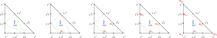
Figure 6: Here we depict the polyhedral embedding of $\mathcal{B}_{0},\ldots,\mathcal{B}_{3}$ into polyhedron 16. The Weierstrass form of the general Newton polynom to polyhedron 16 is calculated in Appendix A1.

6.1 ${\cal O}(-K_{\mathbb{P}^{2}})\rightarrow\mathbb{P}^{2}$

Figure 7: The polyhedron 1. with the modulus $\tilde{u}$

We start by providing the data of the Mori cone

$$\begin{array}[]{c|crrr|rl|}\lx@intercol\hfil\nu_{i}\hfil\lx@intercol&l^{(1)}&\\ D_{u}&&1&0&0&-3&\\ D_{1}&&1&1&0&1&\\ D_{2}&&1&0&1&1&\\ D_{3}&&1&-1&-1&1&\\ \end{array}\,.$$ (6.1)

This gives us the invariant coordinate

$$z=\frac{a_{1}a_{2}a_{3}}{u^{3}}=\frac{1}{\tilde{u}^{3}}.$$ (6.2)

We set $a_{1}=a_{2}=a_{3}=1$ and denote the complex modulus by $\tilde{u}$. Note that the coordinate $z$ is small at the large radius point, whereas the coordinate $\tilde{u}$ is small at the orbifold point. However, from the point of view of embedding the toric diagram of interest into either one of the polygons 13, 15 or 16, it more natural to use the coordinate $\tilde{u}$. As we proceed with blowing up $\mathbb{P}^{2}$ we will always use this coordinate and finally pass to the small coordinate $1/\tilde{u}^{\alpha}$ where $\alpha$ has to be suitably determined.

As explained above instead of starting like in [83] with (3.28) and eliminating $X_{i}$ by (3.29) we solve this equations more geometrically by embedding $\Delta^{*}$ into polyhedra, so that the Newton polyhedron solves immediately the above constraints

$$XY^{2}+YZ^{2}+X^{2}Z+\tilde{u}XYZ=0$$ (6.3)

and yields $H(X,Y)$ by setting $Z=1$. By Nagell’s algorithm its Weierstrass normal form is given by

$$y^{2} = x^{3}+\frac{1}{12}\Big{(}-24\tilde{u}-\tilde{u}^{4}\Big{)}x+\frac{1}{216}\Big{(}-216-36\tilde{u}^{3}-\tilde{u}^{6}\Big{)}\,.$$ (6.4)

It is easy to show that the period integrals $\int_{\gamma}\lambda$ over the meromorphic differential

$$\lambda=\log(x)\frac{dy}{y},$$ (6.5)

which describe the closed string moduli fulfill the differential equations $i=1,\ldots,\#\ {\rm moduli}$

$$\left(\prod_{l^{(i)}_{k}>0}\partial_{a_{k}}^{l^{(i)}_{k}}-\prod_{l^{(k)}_{k}<0}\partial_{a_{k}}^{-l^{(i)}_{k}}\right)\int_{\gamma}\lambda=0\ .$$ (6.6)

The $a_{i}$, $i=1,\ldots,\#\ {\rm points}$ are subject to symmetries of the geometry and can be ‘gauge’-fixed to the variables $z_{i}$ using $a_{i}\partial_{a_{i}}=l_{i}^{(k)}z_{k}\partial_{z_{l}}$. In the case at hand there is just one Picard Fuchs equation (6.6) which has third order

$$\mathcal{L}_{l.r.}=\theta^{3}+3z\theta(3\theta+1)(3\theta+2),$$ (6.7)

where $\theta$ denotes the logarithmic derivative $z\frac{d}{dz}$, s.t. (6.7) reads in terms of $z$

$$\mathcal{L}_{l.r.}=(1+60z)\,\partial_{z}+(3z+108z^{2})\,\partial_{z}^{2}+(z^{2}+27z^{3})\,\partial_{z}^{3}.$$ (6.8)

Recall that the solutions to this differential operator give the periods at the large radius point. As already discussed above, it will often more natural to use the coordinate $\tilde{u}$, in which (6.8) takes the form

$$\mathcal{L}_{orb}=\tilde{u}\,\partial_{\tilde{u}}+3\tilde{u}^{2}\,\partial_{\tilde{u}}^{2}+\left(27+\tilde{u}^{3}\right)\partial_{\tilde{u}}^{3}.$$ (6.9)

The corresponding solutions give the periods at the orbifold point.

We end the discussion of $\mathbb{P}^{2}$ by writing down the prepotential up to degree 7 in $Q_{1}$, denoting ${\rm L}_{\beta}=\text{Li}(Q_{1}^{\beta})$

$$F=\text{class}+3{\rm L}_{1}-6{\rm L}_{2}+27{\rm L}_{3}-192{\rm L}_{4}+1695{\rm L}_{5}-17064{\rm L}_{6}+188454{\rm L}_{7}.$$ (6.10)

The refined invariants have been calculated in [75]. We list a few for reference with the blow-up cases. The connection to our solution of the $\frac{1}{2}K3$ is given by (9.21) and table 6.

d​	​​$j_{L}\backslash j_{R}$​	​​0​	​​​$\frac{1}{2}$​​​	​​​1​​​	​​​$\frac{3}{2}$​​​	​​​2​​​	​​​$\frac{5}{2}$​​​	​​​3​​​	​​​$\frac{7}{2}$​​​	​​​4​​​	​​​$\frac{9}{2}$​​​	​​​5​​​	​​​$\frac{11}{2}$​​​	​​​6​​​	​​​$\frac{13}{2}$​​​	​​​7​​​	​​​$\frac{15}{2}$​​​	​​​8​​​	​​​$\frac{17}{2}$​​​	​​​9​​​	​​​$\frac{19}{2}$​​​	​​​10​​​	​​​$\frac{21}{2}$​​​	​​​11​​​	​​​$\frac{23}{2}$​​​	​​​12​​​	​​​$\frac{25}{2}$​​​	​​​13​​​	​​​$\frac{27}{2}$​​
1​​​	​​​0​​​			​​​1​​​
2​​​	​​​0​​​						​​​1​​​
3​​​	​​​0​​​							​​​1​​​
	​​​$\frac{1}{2}$​​​										​​​1​​​
4​​​	​​​0​​​						​​​1​​​				​​​1​​​				​​​1​​​
	​​​$\frac{1}{2}$​​​									​​​1​​​		​​​1​​​		​​​1​​​
	​​​2​​​												​​​1​​​
	​​​$\frac{3}{2}$​​​															​​​1​​​
5​​​	​​​0​​​			​​​1​​​				​​​1​​​		​​​1​​​		​​​2​​​		​​​2​​​		​​​2​​​		​​​1​​​
	​​​$\frac{1}{2}$​​​						​​​1​​​		​​​1​​​		​​​2​​​		​​​2​​​		​​​3​​​		​​​2​​​		​​​1​​​
	​​​1​​​									​​​1​​​		​​​1​​​		​​​2​​​		​​​2​​​		​​​2​​​		​​​1​​​
	​​​$\frac{3}{2}$​​​												​​​1​​​		​​​1​​​		​​​2​​​		​​​1​​​		​​​1​​​
	​​​2​​​															​​​1​​​		​​​1​​​		​​​1​​​
	​​​$\frac{5}{2}$​​​																		​​​1​​​
	​​​3​​​																					​​​1​​​
6​​​	​​​0​​​		​​​1​​​		​​​1​​​		​​​3​​​		​​​2​​​		​​​6​​​		​​​4​​​		​​​8​​​		​​​5​​​		​​​7​​​		​​​2​​​		​​​2​​​
	​​​$\frac{1}{2}$​​​			​​​1​​​		​​​2​​​		​​​3​​​		​​​5​​​		​​​6​​​		​​​9​​​		​​​9​​​		​​​10​​​		​​​7​​​		​​​5​​​		​​​1​​​		​​​1​​​
	​​​1​​​				​​​1​​​		​​​1​​​		​​​3​​​		​​​3​​​		​​​7​​​		​​​7​​​		​​​11​​​		​​​9​​​		​​​9​​​		​​​4​​​		​​​2​​​
	​​​$\frac{3}{2}$​​​							​​​1​​​		​​​1​​​		​​​3​​​		​​​4​​​		​​​7​​​		​​​7​​​		​​​10​​​		​​​6​​​		​​​4​​​
	​​​2​​​										​​​1​​​		​​​1​​​		​​​3​​​		​​​4​​​		​​​7​​​		​​​6​​​		​​​6​​​		​​​2​​​		​​​1​​​
	​​​$\frac{5}{2}$​​​													​​​1​​​		​​​1​​​		​​​3​​​		​​​3​​​		​​​5​​​		​​​3​​​		​​​2​​​
	​​​3​​​																​​​1​​​		​​​1​​​		​​​3​​​		​​​3​​​		​​​3​​​		​​​1​​​
	​​​$\frac{7}{2}$​​​																			​​​1​​​		​​​1​​​		​​​2​​​		​​​1​​​		​​​1​​​
	​​​​4​​																						​​​1​​​		​​​1​​​		​​​1​​​
	​​​$\frac{9}{2}$​​​																									​​​1​​​
	​​​5​​​																												​​​1​​​
d​	​​$j_{L}/j_{R}$​	​​0​	​​​$\frac{1}{2}$​​​	​​​1​​​	​​​$\frac{3}{2}$​​​	​​​2​​​	​​​$\frac{5}{2}$​​​	​​​3​​​	​​​$\frac{7}{2}$​​​	​​​4​​​	​​​$\frac{9}{2}$​​​	​​​5​​​	​​​$\frac{11}{2}$​​​	​​​6​​​	​​​$\frac{13}{2}$​​​	​​​7​​​	​​​$\frac{15}{2}$​​​	​​​8​​​	​​​$\frac{17}{2}$​​​	​​​9​​​	​​​$\frac{19}{2}$​​​	​​​10​​​	​​​$\frac{21}{2}$​​​	​​​11​​​	​​​$\frac{23}{2}$​​​	​​​12​​​	​​​$\frac{25}{2}$​​​	​​​13​​​	​​​$\frac{27}{2}$​​

Table 3: Non-vanishing BPS numbers $N^{d}_{j_{L},j_{R}}$ of local ${\cal O}(-3)\rightarrow\mathbb{P}^{2}$ up to $d=7$.

6.2 ${\cal O}(-K_{F_{0}})\rightarrow F_{0}$

With the two-parameter model given by the polyhedron 2

Figure 8: The polyhedron 2 with the choice of the mass parameter $m$ and the modulus $\tilde{u}$.

we discuss two perspectives of getting the mirror and perfoming the calculation of the BPS numbers. The first starts with the Mori cone vectors, which correspond to the depicted triangulation

$$\begin{array}[]{ccrrr|rrl|}\lx@intercol\hfil\nu_{i}\hfil\lx@intercol&l^{(1)}&l^{(2)}&\\ D_{u}&&1&0&0&-2&-2&\\ D_{1}&&1&1&0&1&0&\\ D_{2}&&1&0&1&0&1&\\ D_{3}&&1&-1&0&1&0&\\ D_{4}&&1&0&-1&0&1&\\ \end{array}\ .$$ (6.11)

Following (3.28) and eliminating coordinates by (3.29) and the $\mathbb{C}^{*}$-action on the $Y_{i}$ we write the mirror curve in the remaining coordinates $x,y$ as

$$H(x,y)=1+x+\frac{z_{1}}{x}+y+\frac{z_{2}}{y}=0\ ,$$ (6.12)

where the $z_{i}$ are defined as in (3.30). The Picard Fuchs equations (6.6) become in the case at hand with $\theta_{i}:=z_{i}\frac{d}{dz_{i}}$

$$\begin{array}[]{rl}{\cal L}^{(1)}=&\theta_{1}^{2}-2(\theta_{1}+\theta_{2}-1)(2\theta_{1}+2\theta_{2}-1)z_{1}\\ {\cal L}^{(2)}=&\theta_{2}^{2}-2(\theta_{1}+\theta_{2}-1)(2\theta_{1}+2\theta_{2}-1)z_{2}\ .\end{array}$$ (6.13)

Let us come to the discussion of the mass parameter. To make contact with the latter one finds that at $z_{i}=0$ one has a constant solution and two solutions, which are linear in $\log(z_{i})$ and one solution, which is quadratic in $\log(z_{i})$. As the two linear logarithmic solutions one finds $t_{1}=\log(z_{1})+\Sigma(z_{1},z_{2})$ and $t_{2}=\log(z_{2})+\Sigma(z_{1},z_{2})$ determining the Kähler parameters of the $\mathbb{P}^{1}$’s. Here $\Sigma(z_{1},z_{2})$ is the same holomorphic transcendental function. This suggests to change variables and introduce $z=z_{1}$ and $M=\log(z_{1})-\log(z_{2})$. The latter is a trivial solution. We now consider the differential left ideal generated by (6.13) up to homogeneous degree three in differentations w.r.t. $z$ and $M$. In this ideal one can eliminate all differential operators involving derivatives w.r.t. $M$ and end up with a third order differential operator in $z$ determining all non-trivial solutions of (6.13)

$$\begin{array}[]{rl}{\cal L}=&(60\left(m-1\right)^{2}z^{2}-18\left(m+1\right)z+1)\partial_{z}+z\left(80(m-1)^{2}z^{2}-32(m+1)z+3\right)\partial_{z}^{2}+\\ &z^{2}\left(16(m-1)^{2}z^{2}-8(m+1)z+1\right)\partial_{z}^{3}\,.\end{array}$$ (6.14)

Here we understand $m=e^{M}$ now as a deformation parameter. Setting $m=1$ imposes an identification of the complexified Kähler parameters $t_{1}=t_{2}$ globally in the quantum moduli space. This leads to the diagonal model with $S=\mathbb{P}^{1}\times\mathbb{P}^{1}$ as base, discussed in section (D.1). In particular (6.14) restricts for $m=1$ to (5.33) with the appropriate parameters $c_{0}=16$ and $a_{1}=\frac{1}{2},a_{2}=\frac{1}{2}$.

After changes of variables we can parametrize the curve (6.12) as

$$y^{2}+x^{2}-y-\frac{xy}{\sqrt{z}}-mx^{2}y=0$$ (6.15)

and bring it into Weierstrass form (2.11) using Nagell’s algorithm.

Instead of going over the $l^{(k)}$ vectors the elliptic mirror curve is simply associated to the reflexive polyhedron as its Newton polynom, i.e. the coordinates of the points determine its positive exponents. In Appendix A we provide the Newton polynom of the biggest polyhedra so that all polyhedra can be embedded in at least one of them and provide the Weierstrass form for them. In this approach it is only necessary to specialize the general Weierstrass forms and to eventually rescale the $g_{i}\rightarrow g_{i}\lambda^{i}$ to ensure that the closed string period (2.13) has the right leading behaviour. Note that according to the $l$ vectors the right choice of large complex structure coordinates we get from (3.30) is

$$z_{1}=\frac{m}{\tilde{u}^{2}}\quad z_{2}=\frac{1}{\tilde{u}^{2}}$$ (6.16)

so that it is immediatly clear that $z_{1}/z_{2}=m$ and $\tilde{u}\rightarrow\infty$ is the large radius point.

In the $\mathbb{P}^{1}\times\mathbb{P}^{1}$ case we can use the polytop for the cubic or the bi-quartic, the choice does not matter. Let us re-define $u=\frac{1}{\tilde{u}^{2}}=z_{2}$. Then we get

$$\begin{array}[]{rl}g_{2}=&27u^{4}\left(16u^{4}\left(m^{2}-m+1\right)-8u^{2}(m+1)+1\right),\\[5.69054pt] g_{3}=&-27u^{6}(-1+12(1+m)u^{2}-24(2+m+2m^{2})u^{4}+32(2-3m-3m^{2}+2m^{3})u^{6})\ .\end{array}$$ (6.17)

This yields a $j$-invariant

$$j=\frac{\left(16\left(m^{2}-m+1\right)\tilde{u}^{2}-8(m+1)\tilde{u}+1\right)^{3}}{m^{2}\tilde{u}^{4}\left(16(m-1)^{2}\tilde{u}^{2}-8(m+1)\tilde{u}+1\right)}\ .$$ (6.18)

At the large radius we require $t(u,{\underline{m}})=\log(u)+{\cal O}(u,{\underline{m}})$ and near the single zeros of $\Delta$, $t_{c}(u,{\underline{m}})=z_{c}(u,{\underline{m}})+{\cal O}(z_{c}^{2}(u,{\underline{m}}))$, which fixes the scaling (2.14). We have calculated $F^{(n,g)}$ at the conifold to impose the gap condition. Other interesting limits are the Seiberg-Witten limit

$$z_{1}\rightarrow\frac{1}{4}\exp(-4\epsilon^{2}u),\quad z_{2}\rightarrow\epsilon^{4}\Lambda^{4}$$ (6.19)

in which

$$j=\frac{(3\Lambda^{4}-4u^{2})^{3}}{27\Lambda^{8}(\Lambda^{4}-u^{2})}\ .$$ (6.20)

becomes the $j$-function of the massless $SU(2)$ Seiberg-Witten curve compare (6.52) and the Chern-Simons limit discussed for the refined case in [2].

We define a single-valued variable near the large radius as

$$Q_{t}=e^{t}=u+{\cal O}(u^{2},{\underline{m}})\ ,$$ (6.21)

which is easily inverted to $u(Q_{f})$. From Kähler parameters of the two $\mathbb{P}^{1}$’s we define $Q_{i}=e^{t_{i}}$ and get the relation $Q_{t}=Q_{2}$ and $m=Q_{1}/Q_{2}$, which allows us to obtain for all expressions defined in section 2.3 the large radius expansion in terms of $Q_{i}$. The coefficients in (2.18,2.19) are given by $a=7,b=\frac{7}{2},c=-2$ and $d=-1$.

We have calculated the spin invariants and found the following series

$$N^{(1,d)}_{j_{L},j_{R}}=\begin{cases}1&{\rm if}\ \ j_{L}=0,j_{R}=\frac{1}{2}+d\\ 0&{\rm otherwise}\end{cases}$$ (6.22)

Up to $d_{1}+d_{2}\leq 7$ the refined invariants are reported in Table 4.

$(d_{1},d_{2})$​	​​$j_{L}\backslash j_{R}$​	​​0​	​​​$\frac{1}{2}$​​​	​​​1​​​	​​​$\frac{3}{2}$​​​	​​​2​​​	​​​$\frac{5}{2}$​​​	​​​3​​​	​​​$\frac{7}{2}$​​​	​​​4​​​	​​​$\frac{9}{2}$​​​	​​​5​​​	​​​$\frac{11}{2}$​​​	​​​6​​​	​​​$\frac{13}{2}$​​​	​​​7​​​	​​​$\frac{15}{2}$​​​	​​​8​​​	​​​$\frac{17}{2}$​​​	​​​9​​​	​​​$\frac{19}{2}$​​​
$(2,2)$​	​​0​						​​​1​​​		​​​1​​​
	​​$\frac{1}{2}$​									​​​1​​​
$(2,3)$​	​​0​						​​​1​​​		​​​1​​​		​​​2​​​
	​​$\frac{1}{2}$​									​​​1​​​		​​​1​​​
	​​$1$​												​​​1​​​
$(2,4)$​	​​0​						​​​1​​​		​​​1​​​		​​​2​​​		​​​2​​​
	​​$\frac{1}{2}$​									​​​1​​​		​​​1​​​		​​​2​​​
	​​$1$​												​​​1​​​		​​​1​​​
	​​$\frac{3}{2}$​															​​​1​​​
$(2,5)$​	​​0​						​​​1​​​		​​​1​​​		​​​2​​​		​​​2​​​		​​​3​​​
	​​$\frac{1}{2}$​									​​​1​​​		​​​1​​​		​​​2​​​		​​​2​​​
	​​$1$​												​​​1​​​		​​​1​​​		​​​2​​​
	​​$\frac{3}{2}$​															​​​1​​​		​​​1​​​
	​​$2$​																		​​​1​​​
$(3,3)$​	​​0​				​​​1​​​		​​​1​​​		​​​3​​​		​​​3​​​		​​​4​​​
	​​$\frac{1}{2}$​							​​​1​​​		​​​2​​​		​​​3​​​		​​​3​​​		​​​​1​​
	​​$1$​										​​​1​​​		​​​2​​​		​​​3​​​
	​​$\frac{3}{2}$​													​​​1​​​		​​​1​​​
	​​$2$​																​​​1​​​
$(3,4)$​	​​0​		​​​1​​​		​​​1​​​		​​​3​​​		​​​4​​​		​​​7​​​		​​​6​​​		​​​7​​​		​​​1​​​		​​​1​​​
	​​$\frac{1}{2}$​							​​​1​​​		​​​2​​​		​​​4​​​		​​​6​​​		​​​​8​​		​​​2​​​
	​​$1$​								​​​1​​​		​​​2​​​		​​​5​​​		​​​6​​​		​​​7​​​		​​​1​​​
	​​$\frac{3}{2}$​													​​​1​​​		​​​2​​​		​​​4​​​		​​​1​​​
	​​$2$​														​​​1​​​		​​​2​​​		​​​3​​​
	​​$\frac{5}{2}$​																	​​​1​​​		​​​1​​​
	​​$3$​																				​​​1​​​

Table 4: Non-vanishing BPS numbers $N^{(d_{1},d_{2})}_{j_{L},j_{R}}$ of local ${\cal O}(-2,-2)\rightarrow\mathbb{P}^{1}\times\mathbb{P}^{1}$.

6.3 ${\cal O}(-K_{\mathcal{B}_{1}})\rightarrow\mathcal{B}_{1}$

Figure 9: The polyhedron 3 with the choice of the mass parameter $m_{1}$ and the modulus $\tilde{u}$.

The Mori cone is given by

$$\begin{array}[]{cc|crr|rrl|}\lx@intercol\hfil\nu_{i}\hfil\lx@intercol&l^{(1)}=l^{(f)}&l^{(2)}=l^{(b)}&\\ D_{u}&&1&0&0&-2&-1&\\ D_{1}&&1&1&0&1&0&\\ D_{2}&&1&0&1&0&1&\\ D_{3}&&1&-1&0&1&-1&\\ D_{4}&&1&-1&-1&0&1&\\ \end{array}\ .$$ (6.23)

The invariant coordinates are

$$z_{1}=\frac{m}{\tilde{u}^{2}},\quad z_{2}=\frac{1}{\tilde{u}m}.$$ (6.24)

In our choice for the mass parameter we obtain from the embedding

$$XY^{2}+YZ^{2}+X^{2}Z+\tilde{u}XYZ+mXZ^{2}=0$$ (6.25)

and its Weierstrass normal form is given by

$$y^{2} = x^{3}+\frac{1}{12}\Big{(}-24\tilde{u}-\tilde{u}^{4}+8\tilde{u}^{2}m-16m^{2}\Big{)}x{}$$ (6.26)

$$+\frac{1}{216}\Big{(}-216-36\tilde{u}^{3}-\tilde{u}^{6}+144\tilde{u}m+12\tilde{u}^{4}m-48\tilde{u}^{2}m^{2}+64m^{3}\Big{)}\,.$$

As in the $\mathbb{P}^{1}\times\mathbb{P}^{1}$ case, there is a trivial solution to the Picard Fuchs equation that reads

$$\varphi_{1}=\log(z_{1})-2\log(z_{2})=3\log(m).$$ (6.27)

The third order differential operator reads in the case at hand

$${\cal L} = (-12m^{2}+9\tilde{u}-18m\tilde{u}^{2}+8m^{2}\tilde{u}^{3})\partial_{\tilde{u}}+(-108m-128m^{4}+144m^{2}\tilde{u}+27\tilde{u}^{2}{}$$ (6.28)

$$-64m^{3}\tilde{u}^{2}-52m\tilde{u}^{3}+24m^{2}\tilde{u}^{4})\partial_{\tilde{u}}^{2}+(-9+8m\tilde{u})(-27+16m^{3}+36m\tilde{u}{}$$

$$-8m^{2}\tilde{u}^{2}-\tilde{u}^{3}+m\tilde{u}^{4})\partial_{\tilde{u}}^{3}\,.$$

We followed the same logic as in the previous section to get the large radius expansion and obtain the spin invariants. Again there is a series of known numbers

$$N^{(d,1)}_{j_{L},j_{R}}=\begin{cases}1&{\rm if}\ \ j_{L}=0,j_{R}=\frac{2}{d}\\ 0&{\rm otherwise}\end{cases}\,.$$ (6.29)

Note that this equation reduces to the one for the $\mathbb{P}^{2}$ base in the blow-down limit $m=0$. We note that the discriminant reads

$$\Delta=1-\tilde{u}-8m_{1}\tilde{u}^{2}+36m_{1}\tilde{u}^{3}-m_{1}(27-16m_{1})\tilde{u}^{4}\,.$$ (6.30)

The prepotential is given as

$$\begin{array}[]{rl}F=&\text{class}+{\rm L}_{0,1}-2{\rm L}_{1,0}+3{\rm L}_{1,1}+5{\rm L}_{2,1}-6{\rm L}_{2,2}+7{\rm L}_{3,1}-32{\rm L}_{3,2}+27{\rm L}_{3,3}+9{\rm L}_{4,1}\\ &-110{\rm L}_{4,2}+286{\rm L}_{4,3}-192{\rm L}_{4,4}+11{\rm L}_{5,1}-288{\rm L}_{5,2}+1651{\rm L}_{5,3}-3038{\rm L}_{5,4}+1695{\rm L}_{5,5}\\ &+13{\rm L}_{6,1}-644{\rm L}_{6,2}+6885{\rm L}_{6,3}-25216{\rm L}_{6,4}+35870{\rm L}_{6,5}-17064{\rm L}_{6,6}\,.\end{array}$$ (6.31)

Again we have denoted $L_{\beta}=\text{Li}_{3}(Q^{\beta})$. Generally $N^{d_{1},d_{2}}_{j_{L},j_{R}}=0$ for $d_{1}<d_{2}$ and again there is an infinite series of spin invariants that can be given in a closed form

$$N^{(d,1)}_{j_{L},j_{R}}=\begin{cases}1&{\rm if}\ \ j_{L}=0,j_{R}=2d\\ 0&{\rm otherwise}\end{cases}\,.$$ (6.32)

Up to $d_{1}+d_{2}\leq 7$ the refined invariants are reported in Table 5.

$(d_{1},d_{2})$​	​​$j_{L}\backslash j_{R}$​	​​0​	​​​$\frac{1}{2}$​​​	​​​1​​​	​​​$\frac{3}{2}$​​​	​​​2​​​	​​​$\frac{5}{2}$​​​	​​​3​​​	​​​$\frac{7}{2}$​​​	​​​4​​​	​​​$\frac{9}{2}$​​​	​​​5​​​	​​​$\frac{11}{2}$​​​	​​​6​​​	​​​$\frac{13}{2}$​​​	​​​7​​​	​​​$\frac{15}{2}$​​​	​​​8​​​	​​​$\frac{17}{2}$​​​	​​​9​​​	​​​$\frac{19}{2}$​​​
$(2,2)$​	​​0​						​​​1​​​
$(3,2)$​	​​0​						​​​1​​​		​​​1​​​
	​​$\frac{1}{2}$​									​​​1​​​
$(4,2)$​	​​0​						​​​1​​​		​​​1​​​		​​​2​​​
	​​$\frac{1}{2}$​									​​​1​​​		​​​1​​​		​​​1​​​
	​​$1$​														​​​1​​​
$(5,2)$​	​​0​						​​​1​​​		​​​1​​​		​​​2​​​		​​​2​​​
	​​$\frac{1}{2}$​									​​​1​​​		​​​1​​​		​​​2​​​
	​​$1$​												​​​1​​​		​​​1​​​
	​​$\frac{3}{2}$​															​​​1​​​
$(4,3)$​	​​0​					​​​1​​​		​​​​1​​		​​​2​​​		​​​1​​​		​​​1​​​
	​​$\frac{1}{2}$​								​​​1​​​		​​​2​​​		​​​​2​​			​​​​1​​
	​​$1$​											​​​1​​		​​​​1​​
	​​$\frac{3}{2}$​														​​​1​​​	​​​1​​​
$(5,3)$​	​​0​		​​​1​​​		​​​1​​​			​​​3​​​		​​​​3​​		​​​5​​​		​​​​3​​		​​​2​​​
	​​$\frac{1}{2}$​						​​​1​​​		​​​2​​​		​​​4​​​		​​​5​​​		​​​​5​​		​​​1​​​
	​​$1$​									​​1​​​​		​​​2​​​		​​​4​​​		​​​3​​​		​​​1​​​
	​​$\frac{3}{2}$​												​​​1​​​		​​​2​​​		​​​3​​​		​​​1​​​
	​​$2$​															​​​​1​​		​​​1​​​
	​​$\frac{5}{2}$​																			​​​1​​​

Table 5: Non vanishing BPS numbers $N^{(d_{1},d_{2})}_{j_{L},j_{R}}$ of local ${\cal O}(-2,-1)\rightarrow\mathbb{F}_{1}$.

The Seiberg-Witten limit for $\mathbb{F}_{1}$ is

$$z_{1}\rightarrow\frac{1}{4}\exp(-2\sqrt{2}\epsilon^{2}\tilde{u}),\quad z_{2}\rightarrow\epsilon^{4}\Lambda^{4}\ .$$ (6.33)

6.4 ${\cal O}(-K_{\mathbb{F}_{2}})\rightarrow\mathbb{F}_{2}$

We consider the two-parameter model given by the polyhedron 2

Figure 10: The polyhedron 4 with the choice of the mass parameter $m$ and the modulus $\tilde{u}$.

with the Mori cone vectors, which correspond to the depicted triangulation

$$\begin{array}[]{ccrrr|rrl|}\lx@intercol\hfil\nu_{i}\hfil\lx@intercol&l^{(1)}=l^{(f)}&l^{(2)}=l^{(b)}&\\ D_{u}&&1&0&0&-2&0&\\ D_{1}&&1&1&0&1&0&\\ D_{2}&&1&0&1&0&1&\\ D_{3}&&1&-1&0&1&-2&\\ D_{4}&&1&-2&-1&0&1&\\ \end{array}\ .$$ (6.34)

Here we observe a new phenomenon namely a point on the edge, which corresponds to an almost del Pezzo surface. The large structure coordinates are

$$z_{1}=\frac{m}{\tilde{u}^{2}},\qquad z_{2}=\frac{1}{m^{2}}\ .$$ (6.35)

We cannot take simply a ratio between the two coordinates to get the non-dynamical parameter $m$. Let define as before $u=\frac{1}{\tilde{u}^{2}}$, then we find by specialization of (A.9) for the appropriate rescaled $g_{i}$

$$\begin{array}[]{rl}g_{2}=&27u^{4}\left((1-4mu)^{2}-48u^{2}\right),\\[5.69054pt] g_{3}=&-27u^{6}\left(64m^{3}u^{3}-48m^{2}u^{2}-288mu^{3}+12mu+72u^{2}-1\right)\ ,\end{array}$$ (6.36)

which defines $t_{f}$. Let us denote the Kähler parameter of the base $t_{2}$ and the one of the fibre by $t_{1}$. Then we find

$$t_{f}=Q_{1}^{\frac{1}{2}}Q_{2},\quad m=\frac{1+Q_{2}}{Q_{2}^{\frac{1}{2}}}\ .$$ (6.37)

So typically for the almost del Pezzo surfaces we find one transcental mirror map $u(t_{f})$ involving an elliptic integral and rational mirror maps for the mass parameters on the edges. The latter fact is simply due to the fact that the geometry on the edges is a rational geometry involving only Hirzebruch sphere trees of resolved $ADE$ singularities. In fact in the toric case just $A_{n}$-singularities. Now remarkably the spin invariants $N^{\beta}_{j_{l},j_{r}}$ are the same however with a shift in the classes so that $N^{d_{f},d_{b}}_{j_{l},j_{r}}(\mathbb{F}_{2})=N^{d_{f}-d_{b},d_{b}}_{j_{l},j_{r}}(\mathbb{F}_{0})$ and $N^{d_{f},d_{b}}_{j_{l},j_{r}}(\mathbb{F}_{2})=0$ for $d_{f}<d_{b}$.

The Seiberg-Witten limit for $\mathbb{F}_{2}$ is

$$z_{1}\rightarrow\frac{1}{4}\exp(-2\epsilon^{2}\tilde{u}),\quad z_{2}\rightarrow\epsilon^{4}\Lambda^{4}\ .$$ (6.38)

6.5 ${\cal O}(-K_{\mathcal{B}_{2}})\rightarrow\mathcal{B}_{2}$

Figure 11: The polyhedron 5 with the choice of the mass parameter $m_{1},m_{2}$. and the modulus $\tilde{u}$.

The Mori cone is given by

$$\begin{array}[]{cc|crr|rrrl|}\lx@intercol\hfil\nu_{i}\hfil\lx@intercol&l^{(1)}&l^{(2)}&l^{(3)}&\\ D_{u}&&1&0&0&-1&-1&-1&\\ D_{1}&&1&1&0&-1&1&0&\\ D_{2}&&1&1&1&1&-1&1&\\ D_{3}&&1&0&1&0&1&-1&\\ D_{4}&&1&-1&0&0&0&1&\\ D_{5}&&1&0&-1&1&0&0&\end{array}\ .$$ (6.39)

The invariant coordinates are given by

$$z_{1}=\frac{m_{1}m_{2}}{\tilde{u}},\quad z_{2}=\frac{1}{\tilde{u}m_{2}},\quad z_{3}=\frac{m_{2}}{\tilde{u}^{2}}.$$ (6.40)

The mirror curve reads

$$XY^{2}+YZ^{2}+X^{2}Z+\tilde{u}XYZ+m_{1}XZ^{2}+m_{2}X^{2}Y=0$$ (6.41)

and the Weierstrass normal form is given by

$$y^{2} = x^{3}+\frac{1}{12}\Big{(}-24\tilde{u}-\tilde{u}^{4}+8\tilde{u}^{2}m_{1}-16m_{1}^{2}+8\tilde{u}^{2}m_{2}+16m_{1}m_{2}-16m_{2}^{2}\Big{)}x{}$$ (6.42)

$$+\frac{1}{216}\Big{(}-216-36\tilde{u}^{3}-\tilde{u}^{6}+144\tilde{u}m_{1}+12\tilde{u}^{4}m_{1}-48\tilde{u}^{2}m_{1}^{2}+64m_{1}^{3}+144\tilde{u}m_{2}{}$$

$$+12\tilde{u}^{4}m_{2}-24\tilde{u}^{2}m_{1}m_{2}-96m_{1}^{2}m_{2}-48\tilde{u}^{2}m_{2}^{2}-96m_{1}m_{2}^{2}+64m_{2}^{3}\Big{)}.$$

Also in this case a third order differential operator can be constructed. Note however, that in order to derive it one needs two take into account five $l$ vectors out of which only three are linearly independent in order to make the ideal of differential operators close. This is due to the fact that linear dependent relations can give rise to further linear independent differential operators. The full differential operator may be found in the appendix.

Denoting as usual $L_{\beta}=\text{Li}_{3}(Q^{\beta})$, the prepotential is given as

$$\begin{array}[]{rl}F=&\text{class}+{\rm L}_{0,0,1}+{\rm L}_{0,1,0}-2{\rm L}_{0,1,1}+3{\rm L}_{1,1,1}-4{\rm L}_{1,2,1}+5{\rm L}_{1,2,2}-6{\rm L}_{1,3,2}\\ &+7{\rm L}_{1,3,3}-8{\rm L}_{1,4,3}+9{\rm L}_{1,4,4}-6{\rm L}_{2,2,2}+35{\rm L}_{2,3,2}-32{\rm L}_{2,3,3}-32{\rm L}_{2,4,2}\\ &+135{\rm L}_{2,4,3}-110{\rm L}_{2,4,4}+27{\rm L}_{3,3,3}-400{\rm L}_{3,4,3}+286{\rm L}_{3,4,4}-192{\rm L}_{4,4,4}\,.\end{array}$$ (6.43)

Note that there is a symmetry between the first and the third entry, so that we have omitted redundant terms.

6.6 ${\cal O}(-K_{\mathcal{B}_{3}})\rightarrow\mathcal{B}_{3}$

This is the maximal still generic toric blow-up of $\mathbb{P}^{2}$ and is represented by the polyhedron $7$.

Figure 12: The polyhedron 7 with the choice of the mass parameters $m_{1},m_{2},m_{3}$ and the modulus $\tilde{u}$.

The Mori cone vectors, which correspond to the depicted triangulation are given below

$$\begin{array}[]{ccrrr|rrrrrrl|}\lx@intercol\hfil\nu_{i}\hfil\lx@intercol&l^{(1)}&l^{(2)}&l^{(3)}&l^{(4)}&l^{(5)}&l^{(6)}&\\ D_{u}&&1&0&0&-1&-1&-1&-1&-1&-1&\\ D_{1}&&1&1&0&-1&1&0&0&0&1&\\ D_{2}&&1&1&1&1&-1&1&0&0&0&\\ D_{3}&&1&0&1&0&1&-1&1&0&0&\\ D_{4}&&1&-1&0&0&0&1&-1&1&0&\\ D_{5}&&1&-1&-1&0&0&0&1&-1&1&\\ D_{6}&&1&0&-1&1&0&0&0&1&-1&\\ \end{array}\ .$$ (6.44)

One finds the mirror curve

$$XY^{2}+YZ^{2}+X^{2}Z+\tilde{u}XYZ+m_{1}XZ^{2}+m_{2}X^{2}Y+m_{3}Y^{2}Z=0$$ (6.45)

and the Weierstrass normal form

$$y^{2} = 4x^{3}+\frac{1}{12}\Big{(}-16m_{1}^{2}+16m_{1}m_{2}-16m_{2}^{2}+16m_{1}m_{3}+16m_{2}m_{3}-16m_{3}^{2}-24\tilde{u}{}$$ (6.46)

$$-24m_{1}m_{2}m_{3}\tilde{u}+8m_{1}\tilde{u}^{2}+8m_{2}\tilde{u}^{2}+8m_{3}\tilde{u}^{2}-\tilde{u}^{4}\Big{)}{}$$

$$+\frac{1}{216}\Big{(}-216+64m_{1}^{3}-96m_{1}^{2}m_{2}-96m_{1}m_{2}^{2}+64m_{2}^{3}-96m_{1}^{2}m_{3}-48m_{1}m_{2}m_{3}{}$$

$$-96m_{2}^{2}m_{3}-96m_{1}m_{3}^{2}-96m_{2}m_{3}^{2}-216m_{1}^{2}m_{2}^{2}m_{3}^{2}+64m_{3}^{3}+144m_{1}\tilde{u}+144m_{2}\tilde{u}{}$$

$$+144m_{3}\tilde{u}+144m_{1}^{2}m_{2}m_{3}\tilde{u}{}+144m_{1}m_{2}^{2}m_{3}\tilde{u}+144m_{1}m_{2}m_{3}^{2}\tilde{u}-48m_{1}^{2}\tilde{u}^{2}{}$$

$$-24m_{1}m_{2}\tilde{u}^{2}-48m_{2}^{2}\tilde{u}^{2}-24m_{1}m_{3}\tilde{u}^{2}-24m_{2}m_{3}\tilde{u}^{2}-48m_{3}^{2}\tilde{u}^{2}-36\tilde{u}^{3}{}$$

$$-36m_{1}m_{2}m_{3}\tilde{u}^{3}+12m_{1}\tilde{u}^{4}+12m_{2}\tilde{u}^{4}+12m_{3}\tilde{u}^{4}-\tilde{u}^{6}\Big{)}\,.$$

In this case the Mori cone is not simplicial, but we will find a choice of these vectors, which truncates in the correct way to all possibilities of embedding all lower blow up cases into this model. This is only possible by using one non-integer combination of the Mori vectors ${\tilde{l}}^{(1)}=\frac{1}{3}\sum_{i=0}^{2}(l^{(2i+1)}-l^{(2i+2)})$ as well as $\tilde{l}^{(2)}=l^{(2)}$, ${\tilde{l}}^{(3)}=l^{(4)}$ and $\tilde{l}^{(4)}=l^{(6)}$. The corresponding large complex structure variables are

$$z_{1}=m_{1}m_{2}m_{3},\ z_{2}=\frac{1}{m_{1}\tilde{u}},\ z_{3}=\frac{1}{m_{2}\tilde{u}},\ z_{4}=\frac{1}{m_{3}\tilde{u}}\ .$$ (6.47)

We can also calculate the ring of intersection numbers for the choice of basis of curves defined by ${\tilde{l}}^{(i)}$ and the dual divisors $J_{i}$ as

$$R=J_{1}^{2}+J_{1}J_{2}+J_{1}J_{3}+J_{2}J_{3}+J_{1}J_{4}+J_{2}J_{4}+J_{3}J_{4}.$$ (6.48)

With this informations the instantons can be calculated following [71]. Alternatively we can specialize either polyhedron 15 or 16, redefine $\tilde{u}\rightarrow u=1/\tilde{u}$ and rescale $g_{i}\rightarrow\lambda^{i}g_{i}$ with $\lambda=18u^{4}$. Then we obtain the mirror map (2.13) as

$$u=Q_{t}+(1+m_{1})Q_{t}^{3}+2m_{3}Q_{t}^{4}+(1-m_{1}+m_{1}^{2}-3m_{2})Q_{t}^{5}+{\cal O}(Q_{t}^{6})\,.$$ (6.49)

Here we have defined $Q_{t}=e^{t}=(Q_{1}Q_{2}Q_{3}Q_{4})^{\frac{1}{3}}$. It follows from (6.47) that

$$m_{1}=\frac{(Q_{1}Q_{3}Q_{4})^{\frac{1}{3}}}{Q_{2}^{\frac{2}{3}}},\ \ m_{2}=\frac{(Q_{1}Q_{3}Q_{4})^{\frac{1}{3}}}{Q_{3}^{\frac{2}{3}}},\ \ m_{3}=\frac{(Q_{1}Q_{2}Q_{3})^{\frac{1}{3}}}{Q_{4}^{\frac{2}{3}}}.\ \$$ (6.50)

This defines the large radius variables and allows to extract the BPS-numbers directly from the curve. For example we list here the prepotential up to multi-degree 16 in the instantons. With the notation $L_{\beta}={\rm Li}_{3}(Q^{\beta})$ we get

$$\begin{array}[]{rl}F=&\text{class}+{\rm L}_{0,0,0,1}+{\rm L}_{1,0,0,1}-2{\rm L}_{1,0,1,1}+3{\rm L}_{1,1,1,1}+3{\rm L}_{2,1,1,1}-4{\rm L}_{2,1,1,2}+5{\rm L}_{2,1,2,2}\\ &-6{\rm L}_{2,2,2,2}+5{\rm L}_{3,1,2,2}-6{\rm L}_{3,1,2,3}+7{\rm L}_{3,1,3,3}-36{\rm L}_{3,2,2,2}+35{\rm L}_{3,2,2,3}-32{\rm L}_{3,2,3,3}\\ &+27{\rm L}_{3,3,3,3}+7{\rm L}_{4,1,3,3}-8{\rm L}_{4,1,3,4}+9{\rm L}_{4,1,4,4}-6{\rm L}_{4,2,2,2}+35{\rm L}_{4,2,2,3}-32{\rm L}_{4,2,2,4}\\ &-160{\rm L}_{4,2,3,3}+135{\rm L}_{4,2,3,4}-110{\rm L}_{4,2,4,4}+531{\rm L}_{4,3,3,3}-400{\rm L}_{4,3,3,4}+286{\rm L}_{4,3,4,4}\\ &-192{\rm L}_{4,4,4,4}\ .\end{array}$$ (6.51)

Note that there is a symmetry in the last three entries, so that we present only the $\beta$, which are ordered w.r.t these entries.

6.7 Del Pezzos related to the bi-quadratic

Here we want to discuss the remaining polyhedra that are embeddable in the square polyhedron 16 of the bi-quadratic. They are physically interesting e.g. as they correspond to the five-dimensional $SU(2)$ Seiberg-Witten theories with $N_{f}=0,1,2,3,4$ matter multiplets in the fundamental representation. The Seiberg Witten curves with $N_{f}<3$ are given by, see e.g. [39] (also for the $N_{f}=4$ case)

$$y^{2}=(x^{2}-u^{sw})^{2}-\Lambda^{4-N_{f}}\prod_{i=0}^{N_{f}}(x+m^{sw}_{i})\ .$$ (6.52)

The geometry ${\cal O}_{\mathbb{F}_{2}}\rightarrow\mathbb{F}_{2}$ corresponds to one of five-dimensional realization of the $SU(2)$ Seiberg-Witten theory with $N_{f}=0$. The limit in the moduli space, which corresponds to $R=\frac{1}{\epsilon}\rightarrow\infty$, i.e. in which the four-dimensional $SU(2)$ Seiberg-Witten theory emerges was already given in (6.38).

Polyhedron 6 can be viewed as the blow-up of $\mathbb{F}_{2}$ and each blow-up adds one matter in the fundamental representation.

Figure 13: The polyhedron 6 with the choice of the mass parameters $m_{1},m_{2}$ and the modulus $\tilde{u}$.

The Mori cone vectors for this model are

$$\begin{array}[]{ccrrr|rrrl|}\lx@intercol\hfil\nu_{i}\hfil\lx@intercol&l^{(1)}&l^{(2)}&l^{(3)}&\\ D_{u}&&1&0&0&-1&-1&0&\\ D_{1}&&1&1&-1&0&0&1&\\ D_{2}&&1&0&1&1&0&1&\\ D_{3}&&1&-1&0&-1&1&0&\\ D_{4}&&1&-1&-1&1&-1&1&\\ D_{5}&&1&0&-1&0&1&-2&\\ \end{array}\ .$$ (6.53)

From this we get the large volume variables

$$z_{1}=\frac{1}{\tilde{u}m_{2}},\quad z_{2}=\frac{m_{1}m_{2}}{\tilde{u}},\quad z_{3}=\frac{1}{m_{1}^{2}}\,.$$ (6.54)

In this case we define $Q_{t}=Q_{1}^{\frac{1}{2}}Q_{2}Q_{3}^{\frac{1}{4}}$, so that the transcendental mirror map is

$$u=Q_{t}-m_{1}Q_{t}^{3}+2m_{2}Q_{t}^{4}+(-3+m_{1}^{2})Q_{t}^{5}+{\cal O}(Q_{t}^{7})\,.$$ (6.55)

The rational mirror maps are

$$\frac{z_{1}}{z_{2}}=\frac{Q_{1}}{(1+Q_{3})Q_{2}},\quad z_{3}=\frac{Q_{3}}{(1+Q_{3})^{2}}\ .$$ (6.56)

The Seiberg-Witten limit is given by

$$z_{1}=\left(\exp{2^{\frac{2}{3}}}m_{1}^{sw}\epsilon\right),\quad z_{2}=\frac{1}{2}\exp\left(-2^{\frac{2}{3}}\epsilon(2^{\frac{2}{3}}\epsilon u^{sw}+m^{sw}_{1})\right),\quad z_{3}=\Lambda^{3}\epsilon^{3}\ .$$ (6.57)

The first rational Gromov-Witten invariants follow then from a suitable specialization of the biquartic curve (A.21) as

$$\begin{array}[]{rl}F=&\text{class}+L_{1,0,0}+L_{0,1,0}-2L_{1,1,0}+L_{0,1,1}-2L_{1,1,1}+3L_{1,2,1}-4L_{2,2,1}+5L_{2,3,1}\\ &-6L_{3,3,1}+7L_{3,4,1}-8L_{4,4,1}+9L_{4,5,1}-10L_{5,5,1}+11L_{5,6,1}-12L_{6,6,1}+13L_{6,7,1}\\ &+5L_{2,3,2}-6L_{3,3,2}-6L_{2,4,2}+35L_{3,4,2}-32L_{4,4,2}-32L_{3,5,2}+135L_{4,5,2}\\ &-110L_{5,5,2}-110L_{4,6,2}+385L_{5,6,2}-288L_{6,6,2}-288L_{5,7,2}+7L_{3,4,3}-8L_{4,4,3}\\ &-32L_{3,5,3}+135L_{4,5,3}-110L_{5,5,3}+27L_{3,6,3}-400L_{4,6,3}+1100L_{5,6,3}+286L_{4,7,3}\\ &+9L_{4,5,4}-10L_{5,5,4}-110L_{4,6,4}.\end{array}$$ (6.58)

Next we blow it up once more

Figure 14: The polyhedron 9 with the choice of the mass parameters $m_{1},m_{2},m_{3}$ and the modulus $\tilde{u}$.

to get a model with three masses. The new feature we want to discuss here is a non-simplicial Mori cone in a model with rational mirror maps

$$\begin{array}[]{ccrrr|rrrrrl|}\lx@intercol\hfil\nu_{i}\hfil\lx@intercol&l^{(1)}&l^{(2)}&l^{(3)}&l^{(4)}&l^{(5)}&\\ D_{u}&&1&0&0&-1&-1&0&-1&-1&\\ D_{1}&&1&1&-1&0&0&1&-1&1&\\ D_{2}&&1&0&1&1&0&1&0&1&\\ D_{3}&&1&-1&0&-1&1&0&0&0&\\ D_{4}&&1&-1&-1&1&-1&1&0&0&\\ D_{5}&&1&0&-1&0&1&-2&1&0&\\ D_{6}&&1&1&0&0&0&0&1&-1&\\ \end{array}\ .$$ (6.59)

The four large volume coordinates are redundantly given by

$$z_{1}=\frac{1}{{\tilde{u}}m_{2}},\ \ z_{2}=\frac{m_{1}m_{2}}{\tilde{u}},\ \ z_{3}=\frac{1}{\tilde{u}},\ \ z_{4}=\frac{m_{1}m_{3}}{\tilde{u}},\ \ z_{5}=\frac{1}{\tilde{u}m_{3}}\ .$$ (6.60)

These coordinates fulfill the following non-trivial mirror maps $Q_{t}=(Q_{1}Q_{2}Q_{3}Q_{4}Q_{5})^{\frac{1}{4}}$ and

$$z_{3}=\frac{Q_{3}}{(1+Q_{3})^{2}},\ \ \frac{z_{1}}{z_{2}}=\frac{Q_{1}}{Q_{2}(1+Q_{3})},\ \ \frac{z_{5}}{z_{1}}=\frac{Q_{5}}{Q_{4}(1+Q_{3})},\ \ Q_{1}Q_{2}=z_{1}z_{2}=z_{4}z_{5}=Q_{4}Q_{5}\ .$$ (6.61)

To extract the Gromov-Witten invariants from the specialized curve (A.21) we can solve the masses $m_{1},m_{2},m_{3}$ as well as $Q_{t}$ either for $Q_{1},Q_{2},Q_{3},Q_{4}$ or $Q_{2},Q_{3},Q_{4},Q_{5}$, which corresponds to two chambers of the non-simplicial Kähler cone, which are symmetric under the exchange of $Q_{1}Q_{2}\leftrightarrow Q_{4}Q_{5}$ and moreover specialize for $Q_{4}=Q_{5}=0$ to the previously discussed model. In view of the symmetry we list only the invriants for $Q_{1},Q_{2},Q_{3},Q_{4}$

$$\begin{array}[]{rl}F=&\text{class}+L_{0,0,0,1}+L_{0,0,1,1}+L_{0,1,0,0}+L_{0,1,1,0}-2L_{0,1,1,1}+L_{1,0,0,0}-2L_{1,1,0,0}\\ &-2L_{1,1,1,0}+3L_{1,1,1,1}+3L_{1,2,1,0}-4L_{1,2,1,1}-4L_{1,2,2,1}+5L_{1,2,2,2}+5L_{1,3,2,1}\\ &-6L_{1,3,2,2}-4L_{2,2,1,0}+5L_{2,2,1,1}+5L_{2,2,2,1}-6L_{2,2,2,2}+5L_{2,3,1,0}-6L_{2,3,1,1}\\ &+5L_{2,3,2,0}-36L_{2,3,2,1}-6L_{2,4,2,0}-6L_{3,3,1,0}+7L_{3,3,1,1}-6L_{3,3,2,0}+7L_{3,4,1,0}\end{array}\ .$$ (6.62)

Again it is quite interesting to know the Seiberg-Witten limit. We define $z_{f}=z_{1}z_{2}$ and obtain

$$z_{1}=\frac{1}{2}\exp(-2\epsilon m_{1}^{sw}),\ \ z_{f}=\frac{1}{4}\exp(-4\epsilon^{2}u^{sw}),\ \ z_{3}=\Lambda^{2}\epsilon^{2},\ \ z_{4}=\frac{1}{2}\exp(2\epsilon m^{sw}_{2})\ .$$ (6.63)

We finally discuss a model with a simplicial Mori cone, which can be symmetrized like in the last case to the full $D5$ del Pezzo. We performed the calculation, but leave the details to the reader.

Figure 15: The polyhedron 8 with the choice of the mass parameters $m_{1},m_{2},m_{3}$ and the modulus $\tilde{u}$.

The Mori cone vectors determine the large volume variables

$$\begin{array}[]{ccrrr|rrrrl|}\lx@intercol\hfil\nu_{i}\hfil\lx@intercol&l^{(1)}&l^{(2)}&l^{(3)}&l^{(4)}&\\ D_{u}&&1&0&0&0&-1&0&-1&\\ D_{1}&&1&1&-1&1&0&0&0&\\ D_{2}&&1&0&1&0&0&0&1&\\ D_{3}&&1&-1&1&0&0&1&-1&\\ D_{4}&&1&-1&0&0&1&-2&1&\\ D_{5}&&1&-1&-1&1&-1&1&0&\\ D_{6}&&1&0&-1&-2&1&0&0&\\ \end{array}\ .$$ (6.64)

These read in terms of the $m_{i}$ and $\tilde{u}$

$$z_{1}=\frac{1}{m_{1}^{2}},\quad z_{2}=\frac{m_{1}m_{2}}{\tilde{u}},\quad z_{3}=\frac{m_{3}}{m_{2}^{2}},\quad z_{4}=\frac{m_{2}}{\tilde{u}m_{3}}\ .$$ (6.65)

With $Q_{t}=Q_{1}^{\frac{1}{4}}(Q_{2}Q_{3}Q_{4})^{\frac{1}{2}}$ we see as before that the variables $z_{i}$ are not independent transcendental functions of the Kähler parameters rather one has the following relations

$$z_{1}=\frac{Q_{1}}{(1+Q_{1})^{2}},\quad z_{3}=\frac{Q_{3}}{(1+Q_{3})^{2}},\quad z_{2}=\frac{z_{4}(1+Q_{1})Q_{2}}{Q_{4}}\,.$$ (6.66)

$$\begin{array}[]{rl}F=&\text{class}+L_{0,0,0,1}+L_{0,0,1,1}+L_{0,1,0,0}+L_{0,1,1,0}-2L_{0,1,1,1}+L_{1,1,0,0}+L_{1,1,1,0}\\ &-2L_{1,1,1,1}-2L_{1,2,1,0}+3L_{1,2,1,1}+3L_{1,2,2,1}-4L_{1,2,2,2}-4L_{1,3,2,1}+5L_{1,3,2,2}\\ &+5L_{1,3,3,2}-6L_{1,3,3,3}-6L_{1,4,3,2}+7L_{1,4,3,3}+7L_{1,4,4,3}-4L_{2,3,2,1}+5L_{2,3,2,2}\\ &+5L_{2,3,3,2}-6L_{2,3,3,3}+5L_{2,4,2,1}-6L_{2,4,2,2}+5L_{2,4,3,1}-36L_{2,4,3,2}+35L_{2,4,3,3}\\ &-6L_{2,4,4,2}-6L_{2,5,3,1}+35L_{2,5,3,2}-6L_{3,4,3,2}-6L_{3,5,3,1}\,.\end{array}$$ (6.67)

6.8 A mass deformation of the local $E_{8}$ del Pezzo surface

Let us consider the polyhedron $10$.

Figure 16: The polyhedron 10 with the choice of the mass parameters $m_{1},m_{2},m_{3}$ and the modulus $\tilde{u}$.

The Mori cone vectors, which correspond to the depicted triangulation are given below

$$\begin{array}[]{ccrrr|rrrrl|}\lx@intercol\hfil\nu_{i}\hfil\lx@intercol&l^{(1)}&l^{(2)}&l^{(3)}&l^{(4)}&\\ D_{u}&&1&0&0&0&1&0&0&\\ D_{1}&&1&1&0&1&0&0&0&\\ D_{2}&&1&0&1&-2&1&0&0&\\ D_{3}&&1&-1&2&1&-1&1&0&\\ D_{4}&&1&-1&1&0&1&-2&1&\\ D_{5}&&1&-1&0&0&0&1&-2&\\ D_{6}&&1&-1&-1&0&0&0&1&\\ \end{array}\ .$$ (6.68)

With the indicated mass parameters of the three non-renormalizable modes and the para-meter $\tilde{u}$ the Mori vectors determine the large volume $B$-model coordinates

$$z_{1}=\frac{1}{m_{1}^{2}},\ \quad z_{2}=\frac{m_{1}m_{2}}{\tilde{u}},\ z_{3}=\frac{m_{3}}{m_{2}^{2}},\ z_{4}=\frac{m_{2}}{m_{3}^{2}}\ .$$ (6.69)

The anti-canonical class of the $E_{8}$ del Pezzo corresponds to an elliptic curve, which in turn has the following Mori vector

$$l_{e}=3l^{(1)}+6l^{(2)}+4l^{(3)}+2l^{(4)}=\sum_{i}a_{i}l^{(i)}\ .$$ (6.70)

This equation implies that $z_{e}=\frac{1}{u^{6}}=z_{1}^{3}z_{2}^{6}z_{3}^{4}z_{4}^{2}$ is the correct large volume modulus for this curve independently of the masses. By specializing the expression in Appendix A.8 as $m_{1}=0,m_{2}=1,m_{4}=1,m_{6}=1,m_{3}=m_{2},m_{5}=0,a_{1}=0,a_{2}=m_{1},a_{3}=m_{3},\tilde{u}=\frac{1}{u}$ and scaling $g_{i}\rightarrow\lambda^{i}g_{i}$ with $\lambda=18u^{4}$ we get

$$\begin{array}[]{rl}g_{2}=&27u^{4}(24m_{1}u^{3}-48m_{2}u^{4}+16m_{3}^{2}u^{4}-8m_{3}u^{2}+1)\,,\\ g_{3}=&27u^{6}(216m_{1}^{2}u^{6}+12m_{3}u^{2}(-12m_{1}u^{3}+24m_{2}u^{4}-1)+\\ &36m_{1}u^{3}-72m_{2}u^{4}-64m_{3}^{3}u^{6}+48m_{3}^{2}u^{4}-864u^{6}+1)\,.\end{array}$$ (6.71)

The scaling is chosen so that $\frac{dt}{du}=\frac{1}{u}+2m_{3}u+O(u^{2})$ and $t(u,m)$ becomes the logarithmic solution $t(u,m)=\log(u)+{\cal O}(u)$ at infinity $z_{e}=0$, which corresponds to $\frac{1}{j}\sim q\sim u^{6}$. Hence we get as the transcedental mirror map $u=Q_{t}-m_{3}Q_{t}^{3}+{\cal O}(Q_{t}^{4})$, with $Q_{t}=(Q_{e})^{1\over 6}=\sqrt{Q_{1}}Q_{2}Q_{3}^{2\over 3}Q_{4}^{1\over 3}$. The non-transcendental rational mirror maps are

$$z_{1}=\frac{Q_{1}}{(1+Q_{2})^{2}},\ \ z_{3}=Q_{3}\frac{1+Q_{4}+Q_{3}Q_{4}}{(1+Q_{3}+Q_{3}Q_{4})^{2}},\ \ z_{4}=Q_{4}\frac{1+Q_{3}+Q_{3}Q_{4}}{(1+Q_{4}+Q_{3}Q_{4})^{2}}\ .$$ (6.72)

The existence of these rational solutions for the mirror maps can be proven from the system of differential equations that corresponds to the Mori vectors listed above. With the knowledge of these rational solutions the system of differential equations can be reduced to one third order differential equation in $u$ parametrized by the $m_{i}$.

Such rational solutions exist for the differential operators associated to Mori vectors describing the linear relations of points on an (outer) edge of a toric diagram. One can understand their existence from the fact that this subsystem describes effectively a non-compact two-dimensional CY geometry, whose compact part is a Hirzebruch sphere tree, which has no non-trivial mirror maps.

This defines the Kähler parameters of the $A$-model geometry and relates them to the $u,m_{i}$. This allows to extract the BPS invariants for this mass deformation of the $E_{8}$ curve.

7 Local non-rigid geometries

In contrast to the del Pezzo cases we now discuss local geometries which are movable inside the Calabi-Yau space. We start with ${\cal L}_{1}\oplus{\cal L}_{2}\rightarrow\Sigma_{g}$ for $g>0$ and discuss special aspects of the $M$-string geometry.

7.1 Local elliptic curves and quasi-modular forms

Recently, Aganagic et al. [42] have proposed the partition function for the refined topological string on a class of local Calabi-Yau manifolds which are given by two line bundles over a Riemann surface $\mathcal{L}_{1}\oplus\mathcal{L}_{2}\rightarrow\Sigma_{g}$, where $g$ is the genus of the Riemann surface. The Calabi-Yau condition requires the sum of the degrees of the line bundles to be $2g-2$. In the case of genus one, i.e. the Riemann surface $\Sigma_{g}$ is an elliptic curve, we expect the partition function to have some modular properties, which were studied for the unrefined case in e.g. [81, 82].

In the following we consider the Calabi-Yau manifold $\mathcal{O}(1)\oplus\mathcal{O}(-1)\rightarrow\Sigma_{g=1}$. The refined partition function in [42] simplifies to

$$Z(\epsilon_{1},\epsilon_{2},q)=\sum_{R}\exp[\frac{1}{2}(\epsilon_{1}||R||^{2}+\epsilon_{2}||R^{T}||^{2})]q^{|R|},$$ (7.1)

where the sum is over all two-dimensional partitions $R=\{R_{1}\geq R_{2}\geq\cdots\}$. Here $R^{T}$ is the transpose of the partition and the notations are $|R|=\sum_{i}R_{i}$, $||R||^{2}=\sum_{i}(R_{i})^{2}$. $q=e^{-t}$ is the exponential of the Kähler modulus and the small expansion parameter in the large volume limit.

In the unrefined case $\epsilon\equiv\epsilon_{1}=-\epsilon_{2}$, the partition function (7.1) can be written as an infinite product

$$Z(\epsilon,-\epsilon,q)=\textrm{Res}\,\frac{1}{2\pi iz}\prod_{n=1}^{\infty}(1-e^{\frac{(2n-1)^{2}\epsilon}{8}}q^{n-\frac{1}{2}}z)(1-e^{-\frac{(2n-1)^{2}\epsilon}{8}}q^{n-\frac{1}{2}}z^{-1}).$$ (7.2)

We can expand around the small parameter $\epsilon$ and compute the free energy for $g\geq 1$

$$\log(Z(\epsilon,-\epsilon,q))=\sum_{g=1}^{\infty}\epsilon^{2(g-1)}F^{(g)}(q).$$ (7.3)

It is easy to see that the genus one amplitude is given by $F^{(1)}=-\frac{1}{24}\log(\frac{\eta(q)^{24}}{q})$. Here the refined partition function (7.1) only includes the world-sheet instanton contributions, and the $\frac{1}{24}\log(q)$ piece is cancelled by the genus one perturbative contribution so that the total amplitude is modular. For higher genus $g>1$, it was proven in [82] that the amplitudes $F^{(g)}$ are quasi-modular forms of $SL(2,\mathbb{Z})$ of weight $6(g-1)$.

The refined partition function (7.1) is symmetric under the exchange $\epsilon_{1}\leftrightarrow\epsilon_{2}$. However, unlike the cases of del Pezzo and half K3 Calabi-Yau manifolds studied in the previous sections, it is not symmetric under $\epsilon_{1,2}\rightarrow-\epsilon_{1,2}$. As a consequence, the refined Gopakumar-Vafa invariants do not fit in the full $SU(2)_{L}\times SU(2)_{R}$ representations of the five-dimensional little group, and they could be negative integers. We can still expand the logarithm $\log(Z(\epsilon_{1},\epsilon_{2},q))$ as power series of $(\epsilon_{1}+\epsilon_{2})^{n}(\epsilon_{1}\epsilon_{2})^{g-1}$. We find that the coefficients are generally not quasi-modular forms, except for the unrefined amplitudes $F^{(g)}$ in (7.3) and the even power terms in the Nekrasov-Shatashvili limit where one of $\epsilon_{1,2}$ parameters vanishes.

More precisely, we can set $\epsilon_{2}=0$ and $\epsilon\equiv\epsilon_{1}$, and expand the free energy as

$$\log(Z(\epsilon,0,q))=\sum_{n=0}^{\infty}\epsilon^{n}G^{(n)}(q).$$ (7.4)

Here the first term appears also in the unrefined case $G^{(0)}=F^{(1)}=-\frac{1}{24}\log(\frac{\eta(q)^{24}}{q})$. We find that the higher order even terms $G^{(2n)}(q)$ for $n\geq 1$ are quasi-modular forms of weight $6n$. Some formulae at low order read as follows

$$G^{(2)} = \frac{E_{2}E_{4}-E_{6}}{5760},$$

$$G^{(4)} = \frac{-2E_{2}^{3}E_{6}+6E_{2}^{2}E_{4}^{2}-6E_{2}E_{4}E_{6}+E_{4}^{3}+E_{6}^{2}}{1990656},$$

$$G^{(6)} = \frac{1}{5733089280}[99E_{2}^{5}E_{4}^{2}-495E_{2}^{4}E_{4}E_{6}+110E_{2}^{3}(5E_{4}^{3}+4E_{6}^{2})-990E_{2}^{2}E_{4}^{2}E_{6}$$ (7.5)

$$+15E_{2}(13E_{4}^{4}+20E_{4}E_{6}^{2})-79E_{4}^{3}E_{6}-20E_{6}^{3}].$$

It turns out that the proof of the quasi-modularity of the refined amplitudes $G^{(2n)}(q)$ in the Nekrasov-Shatashvili limit is much simpler than that of [82] for the unrefined case, and we can also find explicit formulae for them. First we note that there is also an infinite product formula for (7.1) in the Nekrasov-Shatashvili limit

$$Z(\epsilon,0,q)=\prod_{m=1}^{\infty}(1-e^{\frac{\epsilon^{2}}{2}m^{2}}q^{m})^{-1}.$$ (7.6)

We can then compute the logarithm

$$\log(Z(\epsilon,0,q))=\sum_{m=1}^{\infty}\sum_{k=1}^{\infty}\frac{e^{\frac{\epsilon}{2}km^{2}}q^{km}}{k}=\sum_{l=0}^{\infty}\frac{\epsilon^{l}}{2^{l}l!}\sum_{m=1}^{\infty}\sum_{k=1}^{\infty}k^{l-1}m^{2l}q^{km}.$$ (7.7)

On the other hand, we have the well-known Eisenstein series expansion

$$E_{2n}(q)=1-\frac{4n}{B_{2n}}\sum_{m=1}^{\infty}\sum_{k=1}^{\infty}m^{2n-1}q^{km}.$$ (7.8)

It is now easy to check the explicit formulae for the even power terms in (7.7)

$$G^{(2n)}=-\frac{B_{2n+2}}{2^{2n+2}(n+1)(2n)!}(q\frac{d}{dq})^{2n-1}E_{2n+2}(q)\,.$$ (7.9)

Since the derivative $q\frac{d}{dq}$ preserves the quasi-modularity and increases the modular weight by 2, we see that $G^{(2n)}$ is a quasi-modular form of weight $6n$.

7.2 Modularity in M-Strings and refined constant map contributions

Recently, the elliptic genus of “M-Strings”, constructed by M2-branes suspended between adjacent parallel M5-branes, has been studied in [38]. This is related to the partition function of five-dimensional $N=2^{*}$ $SU(N)$ gauge theory, which is geometrically engineered by topological strings on certain elliptic Calabi-Yau manifolds, given by a deformation of an $A_{N-1}$-fibration over $T^{2}$. The topological partition function can be computed by the refined topological vertex formalism [80]. There are two choices of the preferred direction of the vertices, along the vertical edge or the horizotal edge in the toric diagrams of the Calabi-Yau manifolds. The calculations based on the different choices of the preferred direction should give the same topological partition function, and the equivalence often provides non-trivial identities involving Macdonald polynomials [86].

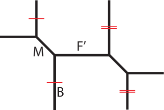
Figure 17: The toric diagram for the five-dimensional ${N}=2^{*}$ $SU(2)$ gauge theory.

Here we consider the case of $SU(2)$ gauge theory. The toric diagram is provided in [38] and displayed here in Figure 17. We see that there are three curve classes $M,B,F^{\prime}$ in the geometry. It is convenient to change basis

$$F=F^{\prime}+M,~{}~{}~{}~{}~{}E=B+M,$$ (7.10)

where $F$ and $E$ denote respectively the fiber and the elliptic curve. In the new basis, the coefficient $r$ in the integral homology class $kF+lE+rM$ can be a negative integer, and the refined BPS invariants may be non-vanishing only in the range $|r|\leq k+l$.

We are interested in the modularity property of the elliptic curve class $E$. We will see that the modularity condition in the class $E$ provides an approach to fix the refinement of the constant map contributions of Gromov-Witten theory. In [38] it has been found that the modularity is manifest if one chooses the preferred direction of the refined vertex to be the horizontal class $F$. The refined BPS invariants for the curve $kF+lE+rM$ with $k>0$ are computed there.

For the case of zero class $F$, i.e. $k=0$, we can choose the vertical edge as preferred direction and set $Q_{f}=0$ in the $SU(2)$ partition function in [38], which becomes

$$Z_{inst}=\big{[}Z^{(1)}\big{]}^{2}.$$ (7.11)

Here the partition function factorizes as square of $Z^{(1)}$, which is the partition function of a single M5-brane wrapped on a circle with mass deformation $m$

$$Z^{(1)}=\sum_{\nu}Q_{\tau}^{|\nu|}\prod_{(i,j)\in\nu}\frac{(1-Q_{m}\,q^{\nu_{j}^{t}-i+\frac{1}{2}}t^{\nu_{i}-j+\frac{1}{2}})(1-Q_{m}^{-1}\,q^{\nu_{j}^{t}-i+\frac{1}{2}}t^{\nu_{i}-j+\frac{1}{2}})}{(1-\,q^{\nu_{j}^{t}-i}t^{\nu_{i}-j+1})(1-\,t^{\nu_{i}-j}q^{\nu_{j}^{t}-i+1})},$$ (7.12)

where $Q_{\tau}$ and $Q_{m}$ are the corresponding exponentials of the Kähler parameters of the classes $E$ and $M$. We are summing over all two-dimensional partitions $\nu$ and the refined parameters are defined by $q=e^{\epsilon_{1}},t=e^{-\epsilon_{2}}$. A different form of the topological partition function, more convenient for extracting the BPS invariants, was given in [86].

We extract the refined BPS invariants from the free energy $F_{inst}=\rm{Log}(Z_{inst})$

$$F_{inst} = -\sum_{j_{L},j_{R}}\sum_{l,r}\sum_{m=1}^{\infty}\frac{(-1)^{2j_{L}+2j_{R}}n^{lE+rM}_{j_{L},j_{R}}}{m(q^{\frac{m}{2}}-q^{-\frac{m}{2}})(t^{\frac{m}{2}}-t^{-\frac{m}{2}})}(Q_{\tau}^{l}Q_{m}^{r})^{m}$$ (7.13)

$$\cdot\frac{(tq)^{-mj_{L}}-(tq)^{mj_{L}+m}}{1-(tq)^{m}}\frac{(\frac{t}{q})^{-mj_{R}}-(\frac{t}{q})^{mj_{R}+m}}{1-(\frac{t}{q})^{m}},$$

and find that the non-vanishing invariants are the following ones

$$n^{lE+M}_{(0,0)}=n^{lE-M}_{(0,0)}=n^{lE}_{(\frac{1}{2},0)}=1,~{}~{}~{}l=1,2,3,\cdots$$ (7.14)

We check the refined BPS invariants to some finite degree $l$, but it may be possible to prove the formulas for all degrees from some ingenious identities of Young diagrams.

We further restrict to the zero mass deformation, i.e. $Q_{m}=1$, and study the modularity in only the $E$-direction. First we consider the unrefined case $q=t$. The BPS invariants in the integer basis $I_{r}=([\frac{1}{2}]+2[0])^{r}$ are

$$\tilde{n}^{lE}_{0}=0,~{}~{}~{}\tilde{n}^{lE}_{1}=1,~{}~{}~{}l=1,2,\cdots$$ (7.15)

The topological free energy is expanded as $F_{inst}=\sum_{g=0}^{\infty}\epsilon^{2g-2}F_{inst}^{(g)}$. For simplicity we consider the modularity of higher genus amplitudes $F^{(g)}$ with $g\geq 2$, which would have positive modular weights. It is straightforward to compute the higher genus amplitudes from the BPS invariants (7.15) as

$$F_{inst}^{(g)}=\tilde{n}^{lE}_{0}\frac{B_{2g}}{2g(2g-2)!}\sum_{d=1}^{\infty}\textrm{Li}_{3-2g}(Q_{\tau}^{d}),~{}~{}~{}~{}g\geq 2.$$ (7.16)

Here only the invariants $\tilde{n}^{lE}_{0}$ contribute to the higher genus amplitudes, while $\tilde{n}^{lE}_{1}=1$ only contribute to the genus one amplitude. The appearance of the polylogarithm function is due to the multi-covering contributions of the BPS invariants, and the Bernoulli numbers $B_{2g}$ come from the familiar expansion

$$\frac{1}{(2\sinh(\frac{\epsilon}{2}))^{2}}=\frac{1}{\epsilon^{2}}-\sum_{g=1}^{\infty}\frac{B_{2g}}{2g(2g-2)!}\epsilon^{2g-2}.$$ (7.17)

The well known constant map contribution in Gromov-Witten theory is

$$C_{g}=\chi\frac{B_{2g}{B_{2g-2}}}{8g(g-1)(2g-2)!},$$ (7.18)

where $\chi$ is the regularized Euler number of the non-compact A-model Calabi-Yau manifold. We see that if we use a regularized Euler number $\chi=\tilde{n}^{lE}_{0}$, the classical constant map contribution and the instanton contribution can nicely combine into Eisenstein series

$$C_{g}+F_{inst}^{(g)}=\chi\frac{B_{2g}{B_{2g-2}}}{8g(g-1)(2g-2)!}E_{2g-2}(Q_{\tau}).$$ (7.19)

Here the case $\chi=0$ is somewhat special, but for more general elliptic Calabi-Yau manifolds with non-vanishing Euler character, this is the mechanism for the quasi-modularity of the topological string amplitudes of zero base class.

We should expect that the nice modularity property generalizes to the refined theory. It turns out to provide a proposal for the refinement of the constant map contribution (7.18), which is different from the one in [80]. First we note the following expansion

$$\frac{1}{(q^{\frac{1}{2}}-q^{-\frac{1}{2}})(t^{\frac{1}{2}}-t^{-\frac{1}{2}})}=-\frac{1}{\epsilon_{1}\epsilon_{2}}+\frac{\epsilon_{1}^{2}+\epsilon_{2}^{2}}{24\epsilon_{1}\epsilon_{2}}-\sum_{g_{1}+g_{2}\geq 2}^{\infty}b_{g_{1}}b_{g_{2}}\epsilon_{1}^{2g_{1}-1}\epsilon_{2}^{2g_{2}-1},$$ (7.20)

where the coefficients are given as $b_{g}=\frac{2^{2g-1}-1}{2^{2g-1}}\frac{B_{2g}}{(2g)!}$. Then the proposal in [80] for the generating function for the higher genus refined constant map contributions is

$$C=\chi\sum_{g_{1}+g_{2}\geq 2}^{\infty}\frac{B_{2g_{1}+2g_{2}-2}}{4(g_{1}+g_{2}-1)}b_{g_{1}}b_{g_{2}}\epsilon_{1}^{2g_{1}-1}\epsilon_{2}^{2g_{2}-1}.$$ (7.21)

Suppose the only non-vanishing refined BPS invariants in the $E$ direction were $n^{lE}_{0,0}=-\chi$, then we could easily see that the classical and instanton contributions for the higher genus refined amplitudes would exactly combine into Eisenstein series, similarly as in the unrefined case.

However this is not the case here, as we see in (7.14) that the non-vanishing refined BPS invariants are actually $n^{lE}_{0,0}=2$ and $n^{lE}_{\frac{1}{2},0}=1$ in the zero mass limit. We can expand the single cover contribution of the BPS states

$$\frac{(tq)^{-\frac{1}{2}}+(tq)^{\frac{1}{2}}-2}{(q^{\frac{1}{2}}-q^{-\frac{1}{2}})(t^{\frac{1}{2}}-t^{-\frac{1}{2}})} = -\frac{(\epsilon_{1}-\epsilon_{2})^{2}}{4\epsilon_{1}\epsilon_{2}}+\frac{(\epsilon_{1}^{2}-\epsilon_{2}^{2})^{2}}{192\epsilon_{1}\epsilon_{2}}-\frac{1}{7680\epsilon_{1}\epsilon_{2}}(\epsilon_{1}^{2}-\epsilon_{2}^{2})^{2}(\epsilon_{1}^{2}+\epsilon_{2}^{2})$$

$$+\frac{1}{15482880\epsilon_{1}\epsilon_{2}}(\epsilon_{1}^{2}-\epsilon_{2}^{2})^{2}(51\epsilon_{1}^{4}+58\epsilon_{1}^{2}\epsilon_{2}^{2}+51\epsilon_{2}^{4})+\mathcal{O}(\epsilon^{8}).$$

We propose the following generating function for the higher genus ($g_{1}+g_{2}\geq 2$) refined constant map contributions

$$C = -\frac{1}{2}[\frac{B_{2}}{2}\frac{(\epsilon_{1}^{2}-\epsilon_{2}^{2})^{2}}{192\epsilon_{1}\epsilon_{2}}-\frac{B_{4}}{4}\frac{1}{7680\epsilon_{1}\epsilon_{2}}(\epsilon_{1}^{2}-\epsilon_{2}^{2})^{2}(\epsilon_{1}^{2}+\epsilon_{2}^{2})$$ (7.22)

$$+\frac{B_{6}}{6}\frac{1}{15482880\epsilon_{1}\epsilon_{2}}(\epsilon_{1}^{2}-\epsilon_{2}^{2})^{2}(51\epsilon_{1}^{4}+58\epsilon_{1}^{2}\epsilon_{2}^{2}+51\epsilon_{2}^{4})+\mathcal{O}(\epsilon^{8})],$$

where we add an overall factor of $-\frac{1}{2}$ and the factor $\frac{B_{2g-2}}{2g-2}$ for the $\epsilon^{2g-2}$ power term. Our proposal for the refined constant map contributions can combine with instanton contributions into Eisenstein series in the present case. Surprisingly, the refined constant map contribution is not proportional to the Euler character, which is effectively zero here and would imply vanishing constant map contributions. As a result, the formula presented here is not universal for general Calabi-Yau manifolds and has to be determined case by case.

8 The half K3 surface: massless theory

We consider the local non-compact Calabi-Yau threefold, constructed by the canonical line bundle over the half K3 surface, similarly as for the del Pezzo surfaces. The half K3 surface can be embedded in an elliptic fibration over a Hirzebruch surface. In our previous paper [77], we studied the refined BPS invariants for the homology classes $p+df$ in $H_{2}(\mathcal{B}_{9},\mathbb{Z})$ , where we wrap the 2-brane once around the base $p$ and $d$ times around the fiber $f$. Here we will further provide the formulae for refined topological string amplitudes in terms of modular forms, and give a refinement of the modular anomaly equation in [74]. The refined modular anomaly equation enables us to compute the refined GV invariants for the more general two-parameter classes $n_{b}p+df$.

The topological string amplitudes on the half K3 Calabi-Yau threefold are equivalent to the partition function of the six-dimensional non-critical E-string compactified on a circle. The winding and momentum numbers of the E-string on the compactified circle correspond to the wrapping numbers $n_{b}$ and $d$ on the base and fiber in the homology classes $n_{b}p+df$ in the half K3 surface.

Recalling the results about intersection form of the homology lattice of the $\frac{1}{2}K3$ from the discussion in 3.1, one finds that the base class $p$ and the fiber class $f$

$$p=[e_{9}],~{}~{}~{}~{}~{}f=3[l]-\sum_{i=1}^{9}[e_{i}]$$ (8.1)

intersect as

$$p\cdot p=-1,~{}~{}~{}p\cdot f=1,~{}~{}~{}f\cdot f=0.$$ (8.2)

In addition to the classes $p$ and $f$, we can turn on eight additional mass parameters corresponding to the other homology classes in $H_{2}(\mathcal{B}_{9},\mathbb{Z})$. The Seiberg-Witten curve description of the prepotential was studied in [5, 62]. The higher genus topological string amplitudes without refinement have been studied e.g. in [73, 92]. The amplitudes have an $E_{8}$ symmetry with respect to the eight mass parameters and can be constructed from the theta functions of the $E_{8}$ lattice, which reduce to modular forms of $SL(2,\mathbb{Z})$ in the massless limit.

In this section we first review the refined Göttsche formula in subsection 8.1, which is an essential ingredient for the refined topological string amplitudes with wrapping number on the base $n_{b}=1$. In the subsections 8.2 and 8.3 we study the massless theory for cases of wrapping number $n_{b}=1$ and $n_{b}>1$, where the (refined) topological string amplitudes can be written in terms of quasi-modular forms of $SL(2,\mathbb{Z})$. In the next section we discuss the refined amplitudes with non-vanishing $E_{8}$ mass parameters.

8.1 The refined Göttsche formula

The Göttsche formula [70] is the generating function for the Betti numbers of the Hilbert scheme of $d$ points on a complex surface $S$. The refinement of the formula appears in [74]. We consider the case of the surface $S$ with Betti numbers $b_{0}(S)=1,b_{1}(S)=0$, which is the case for both, the K3 and the half K3 surfaces. The inverse of the refined formula is an infinite product

$$\frac{1}{G^{S}(q,y_{L},y_{R})} = \prod_{n=1}^{\infty}(1-y_{L}y_{R}q^{n})(1-y_{L}y_{R}^{-1}q^{n})(1-y_{L}^{-1}y_{R}q^{n})(1-y_{L}^{-1}y_{R}^{-1}q^{n})(1-q^{n})^{b_{2}(S)-2}$$ (8.3)

$$= \prod_{n=1}^{\infty}(1-e^{\epsilon_{1}}q^{n})(1-e^{-\epsilon_{1}}q^{n})(1-e^{\epsilon_{2}}q^{n})(1-e^{-\epsilon_{2}}q^{n})(1-q^{n})^{b_{2}(S)-2}\,,$$

where we use the notation $y_{R,L}=\exp(\frac{\epsilon_{1}\pm\epsilon_{2}}{2})$.

The refined product $G^{S}(q,y_{L},y_{R})$ is the generating function for the refinement of the Betti numbers of the Hilbert scheme in the representations of two $SU(2)$ Lefschetz actions

$$G^{S}(q,y_{L},y_{R})=\sum_{d=0}^{\infty}\sum_{j_{L},j_{R}}(-1)^{2j_{L}+2j_{R}}n^{d}_{j_{L},j_{R}}(\sum_{k=-j_{L}}^{j_{L}}y_{L}^{2k})(\sum_{k=-j_{R}}^{j_{R}}y_{R}^{2k})q^{d}.$$ (8.4)

Here $j_{L},j_{R}$ are non-negative half integers labeling the $SU(2)_{L}\times SU(2)_{R}$ representations and we denote $n^{d}_{j_{L},j_{R}}$ as the refined Betti numbers of the Hilbert scheme of $d$ points on $S$.

We can compute the refined Betti numbers from (8.3), (8.4) by plugging in the number for $b_{2}(S)$. We list the refined numbers for the K3 surface ($b_{2}=22$) and the half K3 surface $\mathcal{B}_{9}$ ($b_{2}=10$) in tables 8 and 9. The cases without refinement have been studied in [83] for the K3 surface and in [74, 73] for the half K3 surface. The numbers in tables 8 and 9 reduce to the previous results in the unrefined limit.

More generally in the topological string models, we may multiply the Göttsche product by a modular form of a subgroup of $SL(2,\mathbb{Z})$ and extract the corresponding BPS numbers $n^{d}_{j_{L},j_{R}}$. We mentioned that since the refined BPS invariants count the multiplicity of BPS states without sign, they should be non-negative integers. However we find that this constraint is not very strong, and it is satisfied for a large class of models, e.g. when $b_{2}\geq 2$ and the modular form is a power of the $E_{4}$ Eisenstein series. On the other hand, some BPS numbers become negative when we include the $E_{6}$ series in the modular form. This is because the coefficients in the $E_{4}$ series are positive while they are negative in the $E_{6}$ series. We will see that the topological string amplitudes on the local K3 Calabi-Yau model correspond to the choice of the $E_{4}$ modular form as the pre-factor in the Göttsche product. We speculate that the other choices which give non-negative integers for the refined BPS numbers $n^{d}_{j_{L},j_{R}}$ are possible candidates for consistent refined topological string models.

8.2 Wrapping number on the base $n_{b}=1$

We now consider refined topological string theory on the local half K3 Calabi-Yau, with the wrapping number for the base class $p$ fixed as one. In this case there are no multiple cover contributions within the classes $p+df$. Therefore the genus zero Gromov-Witten invariants are the same as the Gopakumar-Vafa invariants $n_{0}^{p+df}$. The generating function [6] is known to be

$$\sum_{d=0}^{+\infty}n_{0}^{p+df}q^{d}=\frac{q^{\frac{1}{2}}E_{4}(q)}{\eta^{12}(q)}.$$ (8.5)

The higher genus refined GV invariants can be obtained from a generating function $\mathcal{G}(\epsilon_{1},\epsilon_{2},q)$ [77], defined by the product of the genus zero generating function (8.5) and the refined Göttsche formula in (8.3) as follows

$$\mathcal{G}(\epsilon_{1},\epsilon_{2},q)=E_{4}(q)G^{\mathcal{B}_{9}}(q,y_{L},y_{R}).$$ (8.6)

We see that the formula for the generating function $\mathcal{G}(\epsilon_{1},\epsilon_{2},q)$ is an A-model expression. The exponents of $q$ in $\mathcal{G}(\epsilon_{1},\epsilon_{2},q)$ count the self-intersection numbers of the second cohomology classes. In our case the class $p+df$ corresponds to the term $q^{d}$. On the other hand, similar to the formula for the refined Betti numbers in (8.4), the generating function $\mathcal{G}(\epsilon_{1},\epsilon_{2},q)$ can be also expressed in terms of the refined Gopakumar-Vafa invariants

$$\mathcal{G}(\epsilon_{1},\epsilon_{2},q)=\sum_{d=0}^{\infty}\sum_{j_{L},j_{R}}(-1)^{2j_{L}+2j_{R}}n^{p+df}_{j_{L},j_{R}}(\sum_{k=-j_{L}}^{j_{L}}y_{L}^{2k})(\sum_{k=-j_{R}}^{j_{R}}y_{R}^{2k})q^{d},$$ (8.7)

where $j_{L},j_{R}$ take values in the non-negative half integers.

One can extract the refined GV invariants from the equations (8.3, 8.6, 8.7) with the Betti number for half K3 surface $b_{2}(\mathcal{B}_{9})=10$. This was done in our previous paper [77]. Here we also list the integers in table 10 for completeness. We note that the refined GV invariants for the class $p+f$ are the same as the refined GV invariants for the del Pezzo $E_{8}$ for degree $d=1$ displayed in the table in section 5.1. This is expected since the $E_{8}$ is a sub-family in the half K3, and the class $p+f$ in the half K3 corresponds to the class of degree $d=1$ in the del Pezzo $E_{8}$.

The (refined) topological string amplitudes can be expressed in terms of the (refined) GV invariants as explained in (2.8). Due to multiple cover contributions, in general there is no simple relation to compute the topological string amplitude generating function $F(\epsilon_{1},\epsilon_{2},q)$ in (2.9) directly from the Göttsche generating function $\mathcal{G}(\epsilon_{1},\epsilon_{2},q)$, and one has to first compute the (refined) GV invariants as an intermediate step. However, in our case since we only consider the topological string amplitudes for the classes $p+df$ and there is no multiple cover contribution, we can write down a simple relation between the two generating functions

$$F(\epsilon_{1},\epsilon_{2},q)=\frac{\mathcal{G}(\epsilon_{1},\epsilon_{2},q)}{4\sinh(\frac{\epsilon_{1}}{2})\sinh(\frac{\epsilon_{2}}{2})}.$$ (8.8)

It turns out that the higher genus refined topological string amplitudes can be expressed as quasi-modular forms of $SL(2,\mathbb{Z})$. To show this, we first provide an useful identity for the refined Göttsche formula which is the refinement of an identity mentioned in [74],

$$\frac{\epsilon_{1}\epsilon_{2}}{4\sinh(\frac{\epsilon_{1}}{2})\sinh(\frac{\epsilon_{2}}{2})}\prod_{n=1}^{\infty}\frac{(1-q^{n})^{4}}{(1-e^{\epsilon_{1}}q^{n})(1-e^{-\epsilon_{1}}q^{n})(1-e^{\epsilon_{2}}q^{n})(1-e^{-\epsilon_{2}}q^{n})}$$ (8.9)

$$= \exp[-\sum_{k=1}^{\infty}\frac{B_{2k}}{2k(2k)!}(\epsilon_{1}^{2k}+\epsilon_{2}^{2k})E_{2k}(q)].$$

It is a straightforward exercise to demonstrate this identity by taking the logarithm on both sides and using the well-known formula for the Eisenstein series $E_{2k}(q)=1-\frac{4k}{B_{2k}}\sum_{n=1}^{\infty}\frac{n^{2k-1}q^{n}}{1-q^{n}}$.

Utilizing the identity (8.9) and the relation (8.8), we can write the topological string generating function for the class $p+df$ as

$$F(\epsilon_{1},\epsilon_{2},q)=\frac{q^{\frac{1}{2}}E_{4}(q)}{\eta^{12}(q)}\frac{1}{\epsilon_{1}\epsilon_{2}}\exp[-\sum_{k=1}^{\infty}\frac{B_{2k}}{2k(2k)!}(\epsilon_{1}^{2k}+\epsilon_{2}^{2k})E_{2k}(q)].$$ (8.10)

The Eisenstein series $E_{2k}$ for $k\geq 2$ are modular forms of $SL(2,\mathbb{Z})$ and can be written as polynomials of $E_{4}$ and $E_{6}$. $E_{2}$ is quasi-modular, and we can easily see the modular anomaly equation for $F(\epsilon_{1},\epsilon_{2},q)$ with respect to $E_{2}$ from the above formula,

$$\partial_{E_{2}}\log(F(\epsilon_{1},\epsilon_{2},q))=-\frac{\epsilon_{1}^{2}+\epsilon_{2}^{2}}{24},$$ (8.11)

where we have used the Bernoulli number $B_{2}=\frac{1}{6}$. Our modular anomaly equation provides a refinement for the modular anomaly equation in [74] for the class $p+df$.

We can decompose the topological string generating function as in (2.9),

$$F(\epsilon_{1},\epsilon_{2},q)=\sum_{n,g=0}^{+\infty}(\epsilon_{1}+\epsilon_{2})^{2n}(\epsilon_{1}\epsilon_{2})^{g-1}F^{(n,g)}(q),$$ (8.12)

where $F^{(0,g)}$ are the conventional unrefined amplitudes. It is easy to see from (8.10) that the genus zero amplitude is

$$F^{(0,0)}(q)=\frac{q^{\frac{1}{2}}E_{4}(q)}{\eta^{12}(q)}$$ (8.13)

and the higher genus amplitudes divided by the genus zero amplitude $\frac{F^{(n,g)}(q)}{F^{(0,0)}(q)}$ are quasi-modular forms of weight $2(n+g)$. We can write down some explicit formulae at low genus

$$F^{(0,1)}=\frac{E_{2}}{12}F^{(0,0)},~{}~{}~{}F^{(1,0)}=-\frac{E_{2}}{24}F^{(0,0)},~{}~{}~{}F^{(0,2)}=\frac{5E_{2}^{2}+E_{4}}{1440}F^{(0,0)},$$

$$F^{(1,1)}=-\frac{5E_{2}^{2}+2E_{4}}{1440}F^{(0,0)},~{}~{}~{}F^{(2,0)}=\frac{5E_{2}^{2}+2E_{4}}{57600}F^{(0,0)}.$$ (8.14)

The modular anomaly equation (8.11) can be written more explicitly for the higher genus amplitudes as

$$\partial_{E_{2}}F^{(n,g)}=\frac{1}{12}F^{(n,g-1)}-\frac{1}{24}F^{(n-1,g)},$$ (8.15)

where the term $F^{(n,g-1)}$ is defined to be zero if $g=0$, and similarly for $F^{(n-1,g)}$ if $n=0$. We note that this modular anomaly equation seems quite different from the one we used before (5.40). It would be interesting to elucidate the connection.

8.3 Wrapping number on the base $n_{b}>1$

We propose a refinement of the HST modular anomaly equation in [74] as follows

$$\partial_{E_{2}}F^{(n,g,n_{b})} = \frac{1}{24}\sum_{n_{1}=0}^{n}\sum_{g_{1}=0}^{g}\sum_{s=1}^{n_{b}-1}s(n_{b}-s)F^{(n_{1},g_{1},s)}F^{(n-n_{1},g-g_{1},n_{b}-s)}$$ (8.16)

$$+\frac{n_{b}(n_{b}+1)}{24}F^{(n,g-1,n_{b})}-\frac{n_{b}}{24}F^{(n-1,g,n_{b})}.$$

Here $F^{(n,g,n_{b})}$ are the refined topological string amplitudes with wrapping number $n_{b}$ on the base, as appearing in the generating function

$$F=\sum_{n,g,n_{b}=0}^{\infty}(\epsilon_{1}+\epsilon_{2})^{2n}(\epsilon_{1}\epsilon_{2})^{g-1}e^{2\pi it_{b}n_{b}}F^{(n,g,n_{b})}(q),$$ (8.17)

where $t_{b}$ is the Kähler modulus of the base $\mathbb{P}^{1}$, and $q=e^{2\pi i\tau}$ is the modulus of the fiber. It is conjectured that $(\frac{\eta(q)^{12}}{\sqrt{q}})^{n_{b}}F^{(n,g,n_{b})}(q)$ are quasi-modular forms of $SL(2,\mathbb{Z})$ of weight $6n_{b}+2(g+n)-2$, i. e. polynomials of the Eisenstein series $E_{2}(q),E_{4}(q),E_{6}(q)$, so that the partial derivative with respect to $E_{2}$ is well defined.

Our proposal (8.16) reduces to the HST modular anomaly equation [74] in the unrefined case of $n=0$, which can be further reduced by setting $g=0$ to the genus zero equation studied earlier in [4]. The generalizations to more elliptic Calabi-Yau manifolds have been studied recently in [44, 84]. The genus zero prepotential with base wrapping number $n_{b}$ is also equivalent to the partition function of topological ${N}=4$ $U(n_{b})$ super Yang-Mills theory [7]. Another special case is the case of wrapping number $n_{b}=1$ studied in the previous subsection 8.2, where our proposal becomes the equation (8.15) derived there. We have guessed the factor $\frac{n_{b}}{24}$ in the last term in (8.16) by trials and tested by higher genus calculations, which we now discuss.

We can solve the higher genus refined amplitudes recursively in $n,g,n_{b}$ by integrating the refined holomorphic anomaly equation. The integration constant is a polynomial of $E_{4}(q)$ and $E_{6}(q)$, and needs to be fixed by some boundary conditions. Here we will not use the gap conditions at the conifold locus, because it would require a careful analysis of the moduli space, which is quite complicated in multi-parameter models. Instead, we will utilize the boundary conditions due to vanishing GV invariants. We have mentioned before that if a GV integer vanishes $\tilde{n}^{\beta}_{g_{L},g_{R}}=0$, then the higher genus neighbors also vanish $\tilde{n}^{\beta}_{g_{L}+1,g_{R}}=\tilde{n}^{\beta}_{g_{L},g_{R}+1}=0$. In addition, at genus zero it is also known [6] that the GV invariants vanish $\tilde{n}^{n_{b}p+df}_{0,0}=0$ if $n_{b}>d$, except for the case of $n_{b}=1,d=0$ where we have $\tilde{n}^{p}_{0,0}=1$. The property was used in [4] to fix the integration constants for the genus zero modular anomaly equation.

In the special case of $n_{b}=1$ studied in the previous subsection 8.2, the integration of the modular anomaly equation by fixing the integration constants by vanishing GV invariants leads to a nice A-model type formula (8.8), related to the refined Göttsche formula (8.3). The A-model type formulae are exact to all genera, and are rather convenient for extracting the complete GV invariants $n^{\beta}_{j_{L},j_{R}}$ for a fixed homology class $\beta$. Here in the general case with wrapping number $n_{b}>1$, the A-model type formula is currently not available and therefore B-model calculations need to be done in order to extract the BPS invariants recursively.

We are able to compute the refined topological string amplitudes to some high genus $n+g$ and some high wrapping number $n_{b}$, and we can extract the complete refined GV invariants to some high degree for the base $n_{b}$ and fiber. We provide some refined amplitudes $F^{(n,g,n_{b})}$ for low genus $n+g$ and wrapping number $n_{b}\geq 2$. The genus zero amplitudes [4] for $n_{b}=2,3$ are

$$F^{(0,0,2)}=\frac{q}{\eta(q)^{24}}\frac{E_{4}}{24}(E_{2}E_{4}+2E_{6}),$$ (8.18)

$$F^{(0,0,3)}=\frac{q^{\frac{3}{2}}}{\eta(q)^{36}}\frac{E_{4}}{15552}(54E_{2}^{2}E_{4}^{2}+216E_{2}E_{4}E_{6}+109E_{4}^{3}+197E_{6}^{2}).$$

The genus one amplitudes for $n_{b}=2,3$ are

$$F^{(0,1,2)}=\frac{q}{\eta(q)^{24}}\frac{1}{1152}(10E_{2}^{2}E_{4}^{2}+9E_{4}^{3}+24E_{2}E_{4}E_{6}+5E_{6}^{2}),$$ (8.19)

$$F^{(1,0,2)}=-\frac{q}{\eta(q)^{24}}\frac{1}{1152}(4E_{2}^{2}E_{4}^{2}+7E_{4}^{3}+8E_{2}E_{4}E_{6}+5E_{6}^{2}),$$

$$F^{(0,1,3)}=\frac{q^{\frac{3}{2}}}{\eta(q)^{36}}\frac{78E_{2}^{3}E_{4}^{3}+299E_{2}E_{4}^{4}+360E_{2}^{2}E_{4}^{2}E_{6}+472E_{4}^{3}E_{6}+439E_{2}E_{4}E_{6}^{2}+80E_{6}^{3}}{62208},$$

$$F^{(1,0,3)}=-\frac{q^{\frac{3}{2}}}{\eta(q)^{36}}\frac{54E_{2}^{3}E_{4}^{3}+235E_{2}E_{4}^{4}+216E_{2}^{2}E_{4}^{2}E_{6}+776E_{4}^{3}E_{6}+287E_{2}E_{4}E_{6}^{2}+160E_{6}^{3}}{124416}.$$

The genus two amplitudes for $n_{b}=2$ are

$$F^{(0,2,2)}=\frac{q}{\eta(q)^{24}}\frac{190E_{2}^{3}E_{4}^{2}+417E_{2}E_{4}^{3}+540E_{2}^{2}E_{4}E_{6}+356E_{4}^{2}E_{6}+225E_{2}E_{6}^{2}}{207360},$$

$$F^{(1,1,2)}=-\frac{q}{\eta(q)^{24}}\frac{25E_{2}^{3}E_{4}^{2}+79E_{2}E_{4}^{3}+60E_{2}^{2}E_{4}E_{6}+122E_{4}^{2}E_{6}+50E_{2}E_{6}^{2}}{34560},$$

$$F^{(2,0,2)}=\frac{q}{\eta(q)^{24}}\frac{10E_{2}^{3}E_{4}^{2}+37E_{2}E_{4}^{3}+20E_{2}^{2}E_{4}E_{6}+76E_{4}^{2}E_{6}+25E_{2}E_{6}^{2}}{69120}.$$ (8.20)

We list some results for refined BPS invariants for $n_{b}>1$ in the tables 11 and 12. The diagonal classes $n_{b}(p+f)$ correspond to the homology classes with degrees $d=n_{b}$ in the one-parameter $E_{8}$ del Pezzo model, and we check the matching of the corresponding BPS integers for the diagonal classes $n_{b}(p+f)$ with those in section 5.1. Our results demonstrate the compatibility of the refined version of the HST modular anomaly equation we proposed in (8.16) with the refined version of the BCOV holomorphic anomaly equation in (5.40).

In two special cases, namely the genus zero case $n+g=0$ and the case of wrapping number $n_{b}=1$, it is clear that one can in principle solve the refined topological strings to all orders in the other directions, i.e. to all orders in $n_{b}$ in the case of $n+g=0$ and all orders in $n,g$ in the case of $n_{b}=1$. It is tempting to wonder whether the vanishing conditions for GV invariants are sufficient in principle to fix the topological string amplitudes to all orders in both $n+g$ and $n_{b}$. Unfortunately this is not the case, even for the unrefined case $n=0$. The integration constant for the modular anomaly equation for $F^{(n,g,n_{b})}$ is a polynomial of $E_{4}$ and $E_{6}$ of weighted degree $2(n+g)+6n_{b}-2$, so the number of unknown constant we need to fix is given by $[\frac{2(n+g)+6n_{b}-2}{12}]$ for odd $n+g+n_{b}$, or by $[\frac{2(n+g)+6n_{b}-8}{12}]$ for even $n+g+n_{b}$. On the other hand, we can also estimate the number of vanishing GV invariants $\tilde{n}_{g_{L},g_{R}}^{n_{b}p+df}$ for given $n_{b},g_{L},g_{R}$. It is clear that the GV invariants vanish for $d<n_{b}$ since the genus zero invariants already vanish $\tilde{n}_{0,0}^{n_{b}p+df}=0$ if $d<n_{b}$. Based on arguments from algebraic geometry, e.g. in [83, 78], we know that the left top genus for the diagonal class $n_{b}p+n_{b}f$ goes like quadratic power $n_{b}^{2}$ for large $n_{b}$, and this is also confirmed by our explicit results. The GV invariant $\tilde{n}_{g_{L},g_{R}}^{n_{b}(p+f)}$ would not vanish if the total genus $g_{L}+g_{R}$ scaled as quadratic power $n_{b}^{2}$ at large $n_{b}$ but was smaller than the left top genus. In this case we would have just $n_{b}$ vanishing GV invariants $\tilde{n}_{0,0}^{n_{b}p+df}$ from $d=0,1,\cdots,n_{b}-1$, but the number of unknown constants could be of the order of the quadratic power $n_{b}^{2}$ at large $n_{b}$. So eventually the boundary conditions from vanishing GV invariants would not be enough to fix the (refined) topological string amplitudes at large genus.

In fact, we can be a little more precise and show that the situation regarding fixing the ambiguity for the diagonal classes $n_{b}(p+f)$ is not better or worse than that of the $E_{8}$ model. This is rather surprising because in the case of the $E_{8}$ model we have utilized the conifold gap condition which is very powerful in fixing the holomorphic ambiguity, while in the half K3 model we do not use the conifold gap condition. In the $E_{8}$ model, we have $[\frac{2(n+g)-2}{6}]$ unknown constants in the holomorphic ambiguity in $F^{(n,g)}$ due to the singularity at the orbifold point. Suppose for the genus $g_{L}+g_{R}=n+g$ we can fix the (refined) GV invariants $\tilde{n}^{\beta}_{g_{L},g_{R}}$ up to degree $d-1$, then in this case the number of conditions from GV invariants minus the number of unknown constants is $d-1-[\frac{2(n+g)-2}{6}]$. On the other hand, for the refined amplitude $F^{(n,g,n_{b})}$ with $n_{b}=d$ in the half K3 model, based on the discussions in the previous paragraph, we can easily check that the number of conditions from GV invariants minus the number of ambiguous constants is up to $\pm 1$ basically $\frac{1}{2}(d-1-[\frac{2(n+g)-2}{6}])$, i.e. one half of that of the $E_{8}$ model. So we see that the boundary conditions from GV invariants become insufficient to fix the ambiguity at about the same time for the $E_{8}$ model and for the diagonal classes in the half K3 model.

These arguments indicate that the vanishing of BPS invariants in the two-parameter half K3 model should imply the conifold gap conditions in the one-parameter $E_{8}$ model. It would interesting to understand this point more carefully.

9 The half K3 surface: massive theory

Based on the experience from the studies of higher genus terms in the Nekrasov function for $SU(2)$ Seiberg-Witten theory with $N_{f}=4$ fundamental flavors or with one adjoint hypermultiplet in [75], we may hope that the mass deformation provides more boundary conditions for fixing the ambiguity comparing to the massless theory. There is one crucial difference with the studies in [75], where the mass parameters are not moduli parameters, and there is no enumerative geometric interpretation of the refined amplitudes in terms of the BPS invariants. In the present case, the mass parameters represent Kähler moduli of the $E_{8}$ part of the half K3 surface, and are part of the geometry of the moduli space. The refined BPS invariants have extra labels in terms of the corresponding wrapping degrees which are Weyl orbits of the $E_{8}$ lattice. In the mirror geometry, the mass parameters appear as polynomials in the Seiberg-Witten curve in [75], and in the present case they appear in exponential or trigonometric functions. This point was explained in [5].

We will need to use the theta function of the $E_{8}$ lattice $\Gamma_{8}$

$$\Theta(\vec{m},\tau)=\sum_{\vec{w}\in\Gamma_{8}}\exp(\pi i\tau\vec{w}^{2}+2\pi i\vec{m}\cdot\vec{w})=\frac{1}{2}\sum_{k=1}^{4}\prod_{j=1}^{8}\theta_{k}(m_{j},\tau)\,,$$ (9.1)

where $\vec{m}=(m_{1},m_{2},\cdots,m_{8})$ are the $E_{8}$ mass parameters. $\theta_{k}(m,\tau)$ is the ordinary Jacobi theta function and we provide the conventions in appendix C. The theta function $\Theta(\vec{m},\tau)$ of the $E_{8}$ lattice is a power series in $q=e^{2\pi i\tau}$, and from the well-known transformation properties of Jacobi theta functions, one can check that it has the following transformation behavior under a $SL(2,\mathbb{Z})$ transformation

$$\Theta(\frac{\vec{m}}{c\tau+d},\frac{a\tau+b}{c\tau+d})=(c\tau+d)^{4}\exp(\frac{i\sum_{i}m_{i}^{2}}{c\tau+d})\Theta(\vec{m},\tau).$$ (9.2)

We see that except for the modular phase, it has modular weight four under the $SL(2,\mathbb{Z})$ transformation. Furthermore, in the massless limit $\vec{m}=0$, the theta function $\Theta(\vec{m},\tau)$ is simply the $E_{4}$ Eisenstein series.

One can easily see that the $E_{8}$ theta function (9.1) is invariant under a Weyl group action on the mass vector $\vec{m}$ since the lattice $\Gamma_{8}$ and the norm of a lattice vector are invariant under the action.

The Weyl orbit of a lattice vector consists of the lattice vectors generated by acting all the elements of the Weyl group $W(E_{8})$ on the lattice vector. We can classify the $E_{8}$ lattice points into classes of Weyl orbits. It is clear that the lattice vectors in the same Weyl orbit have the same norm. We denote by $\mathcal{O}_{p,k}$ the Weyl orbit whose element $\vec{w}$ has norm square $\vec{w}\cdot\vec{w}=2p$ and which has order $|\mathcal{O}_{p,k}|=k$. Since the Weyl orbits of the same norm usually have different numbers of elements, the notation should not cause any confusion. It is known that some low Weyl orbits are given as follows

$$\mathcal{O}_{0,1},~{}~{}\mathcal{O}_{1,240},~{}~{}\mathcal{O}_{2,2160},~{}~{}\mathcal{O}_{3,6720},~{}~{}\mathcal{O}_{4,240},\mathcal{O}_{4,17280},~{}~{}\mathcal{O}_{5,30240}$$

$$\mathcal{O}_{6,60480},~{}~{}\mathcal{O}_{7,13440},\mathcal{O}_{7,69120},~{}~{}\mathcal{O}_{8,2160},\mathcal{O}_{8,138240},~{}~{}\mathcal{O}_{9,240},\mathcal{O}_{9,181440},~{}~{}$$

$$\mathcal{O}_{10,30240},\mathcal{O}_{10,241920},~{}~{}\mathcal{O}_{11,138240},\mathcal{O}_{11,181440},~{}~{}\mathcal{O}_{12,6720},\mathcal{O}_{12,483840},$$

$$\mathcal{O}_{13,13440},\mathcal{O}_{13,30240},\mathcal{O}_{13,483840},~{}~{}\cdots.$$ (9.3)

We see that the lattice vectors with norm square $0,2,4,6,10,12$ consist of a single Weyl orbit respectively, while the lattice vectors with norm square $8,14,16,18,20,\cdots$ fall into multiple orbits. Any Weyl orbit $\mathcal{O}_{p,k}$ can be multiplied with a positive integer $n$ and generates another Weyl orbit with the same order $\mathcal{O}_{n^{2}p,k}=\{n\vec{w}|~{}\vec{w}\in\mathcal{O}_{p,k}\}$.

The $E_{8}$ theta function (9.1) can be written as sums over Weyl orbits

$$\Theta(\vec{m},q)=\sum_{\mathcal{O}_{p,k}}q^{p}\sum_{\vec{w}\in\mathcal{O}_{p,k}}\exp(2\pi i\vec{m}\cdot\vec{w}),$$ (9.4)

where $q=e^{2\pi i\tau}$. We will see that the (refined) topological string amplitudes in the massive half K3 model are constructed from the $E_{8}$ theta function, and can be also written as sums over the Weyl orbits. The refined BPS invariants are labelled by the class $n_{b}p+df$ and the Weyl orbit $\mathcal{O}_{p,k}$, and denoted as $n^{n_{b}p+df,\mathcal{O}_{p,k}}_{j_{L},j_{R}}$. We can compute the refined amplitudes in terms of refined BPS invariants with the formula (2.8) and by summing over the homology classes $\beta=(n_{b}p+df,\mathcal{O}_{p,k})$. As in the massless theory we denote the refined amplitudes by $F^{(n,g,n_{b})}(q,\vec{m})$ as appearing in the generating function in (8.17). The arguments $q$ and $\vec{m}$ represent the Kähler moduli of the fiber class $f$ and Weyl orbits.

In the massless limit, the sum over a Weyl orbit $\mathcal{O}_{p,k}$, is simply the order $|\mathcal{O}_{p,k}|=k$. So the refined BPS invariants in the massless limit can be computed from the more general massive invariants by

$$(n^{n_{b}p+df}_{j_{L},j_{R}})_{massless}=\sum_{\mathcal{O}_{p,k}}k\cdot n^{n_{b}p+df,\mathcal{O}_{p,k}}_{j_{L},j_{R}}\,.$$ (9.5)

First we consider the case of wrapping number $n_{b}=1$. In this case the refined Göttsche formula is still available as in the massless theory. We can simply replace the Eisenstein series $E_{4}$ with the theta function $\Theta(\vec{m},\tau)$ for the generating function in (8.6) in the massless theory

$$\mathcal{G}(\epsilon_{1},\epsilon_{2},q)=\Theta(\vec{m},q)G^{\mathcal{B}_{9}}(q,y_{L},y_{R}).$$ (9.6)

Using the formula for the $E_{8}$ theta function (9.4), we find

$$\mathcal{G}(\epsilon_{1},\epsilon_{2},q) = \sum_{d=0}^{\infty}\sum_{\mathcal{O}_{p,k}}\sum_{j_{L},j_{R}}(-1)^{2j_{L}+2j_{R}}(n^{\mathcal{B}_{9}})^{d}_{j_{L},j_{R}}(\sum_{k=-j_{L}}^{j_{L}}y_{L}^{2k})(\sum_{k=-j_{R}}^{j_{R}}y_{R}^{2k})$$ (9.7)

$$\times q^{d+p}\sum_{\vec{w}\in\mathcal{O}_{p,k}}\exp(2\pi i\vec{m}\cdot\vec{w}).$$

We can then extract the refined Gopakumar-Vafa BPS invariants similarly as in (8.7) for the massless theory, with the additional sum over Weyl orbits

$$\mathcal{G}(\epsilon_{1},\epsilon_{2},q) = \sum_{d=0}^{\infty}\sum_{\mathcal{O}_{p,k}}\sum_{j_{L},j_{R}}(-1)^{2j_{L}+2j_{R}}n^{p+df,\mathcal{O}_{p,k}}_{j_{L},j_{R}}(\sum_{k=-j_{L}}^{j_{L}}y_{L}^{2k})(\sum_{k=-j_{R}}^{j_{R}}y_{R}^{2k})$$ (9.8)

$$\times q^{d}\sum_{\vec{w}\in\mathcal{O}_{p,k}}\exp(2\pi i\vec{m}\cdot\vec{w}),$$

where the sums over $j_{L},j_{R}$ are over non-negative half integers. To extract the BPS integers, we first use the formula (8.4) to write the Göttsche product $G^{\mathcal{B}_{9}}(q,y_{L},y_{R})$ in terms of the refined Betti numbers of the Hilbert schemes which have been computed in table 9, and which we denote here by $(n^{\mathcal{B}_{9}})^{d}_{j_{L},j_{R}}$ with the superscript $\mathcal{B}_{9}$ to avoid confusion with other BPS invariants.

Comparing (9.7) and (9.8), we find the BPS invariants in terms of the refined Betti numbers

$$n^{p+df,\mathcal{O}_{p,k}}_{j_{L},j_{R}}=(n^{\mathcal{B}_{9}})^{d-p}_{j_{L},j_{R}},~{}~{}~{}\textrm{for}~{}p\leq d$$ (9.9)

and it is understood that $n^{p+df,\mathcal{O}_{p,k}}_{j_{L},j_{R}}=0$ in the case of $p>d$.

We see from the formula (9.9) that the refined BPS invariants $n^{p+df,\mathcal{O}_{p,k}}_{j_{L},j_{R}}$ are identical for the homology classes with the same $d-p$. Furthermore for a class $p+df$, the refined BPS invariants vanish if the square length for the Weyl orbits are sufficiently large. The Weyl orbit with maximal length and non-vanishing BPS invariants will be called the top Weyl orbit(s). Here the top Weyl orbit for the class $p+df$ is the orbit $\mathcal{O}_{d,k}$.

As a check of the formalism, we can compute the refined BPS invariants for the half K3 model in the massless limit using the formula (9.5) and the Weyl orbits (9), in terms of the refined Betti numbers in table 9. The results agree with those from direct calculations in table 10. This is simply due to the fact that the $E_{8}$ theta function $\Theta(\vec{m},q)$ is the Eisenstein series $E_{4}$ in the massless limit.

Similarly as in the massless theory, we can write down the genus zero amplitude for $n_{b}=1$ by setting $y_{L}=y_{R}=1$ in the Göttsche product

$$F^{(0,0,1)}=\frac{q^{\frac{1}{2}}\Theta(\vec{m},q)}{\eta(q)^{12}}.$$ (9.10)

The formulae for the refined higher genus amplitudes and the modular anomaly equation for $n_{b}=1$ are the same as in the massless theory in (8.2), (8.15).

Now we consider the case of wrapping number $n_{b}>1$. The higher genus refined amplitude with an $\eta$ function factor $(\frac{\eta(q)^{12}}{\sqrt{q}})^{n_{b}}F^{(n,g,n_{b})}$ has modular weight $2(n+g)+6n_{b}-2$ as in the massless theory. However, the modular ambiguity is not simply a modular form of $SL(2,\mathbb{Z})$. Instead, the modular ambiguity can be written as a linear combination of level $n_{b}$ $E_{8}$ characters, and the coefficients are mass-independent modular forms of $\Gamma_{1}(n_{b})$ [7].

There is a convenient way to write the ansatz for the refined amplitudes. It is known that there are nine Weyl invariant Jacobi modular forms of the $E_{8}$ lattice, which can be constructed from the $E_{8}$ theta function (9.1), see e.g. [92]. The nine Jacobi forms are denoted by $A_{1},A_{2},A_{3},A_{4},A_{5}$ and $B_{2},B_{3},B_{4},B_{6}$. Here $A_{1}=\Theta(\vec{m},\tau)$ is simply the $E_{8}$ theta function and we provide the detailed formulae for the other forms in appendix C. All the characters of the fundamental representation of the higher level $E_{8}$ algebra can then be written as polynomials in $A_{n}$ and $B_{n}$, where the generators $A_{n}$ or $B_{n}$ contribute an $E_{8}$ level number $n$. For example, at level one there is only one polynomial $A_{1}$. There are three polynomials $A_{1}^{2},A_{2},B_{2}$ at level two, five polynomials $A_{1}^{3},A_{1}A_{2},A_{1}B_{2},A_{3},B_{3}$ at level three, and ten polynomials at level four.

The Jacobi form $A_{n}$ has modular weight four and $B_{n}$ has modular weight six, and they are simply the Eisenstein series $E_{4}$ and $E_{6}$ in the massless limit. Together with the quasi-modular forms $E_{2},E_{4},E_{6}$ of $SL(2,\mathbb{Z})$ which are independent of the mass parameters and have $E_{8}$ level number zero, we have all the ingredients for constructing the refined amplitudes.

It is natural to guess that similarly as in the massless theory, the scaled refined amplitude with $\eta$ function factor $(\frac{\eta(q)^{12}}{\sqrt{q}})^{n_{b}}F^{(n,g,n_{b})}$ can be written as polynomials of the nine $E_{8}$ Jacobi forms $A_{n}$, $B_{n}$ and the $SL(2,\mathbb{Z})$ quasi-modular forms $E_{2}$, $E_{4}$, $E_{6}$, and it has $E_{8}$ level number $n_{b}$ and modular weight $2(n+g)+6n_{b}-2$. We find that this is true for level $n_{b}\leq 4$. However, for level $n_{b}\geq 5$, the scaled amplitude $(\frac{\eta(q)^{12}}{\sqrt{q}})^{n_{b}}F^{(n,g,n_{b})}$ is not exactly a modular form, but a rational function of modular forms with the powers in $E_{4}$ as the denominator. For example for the case of $n_{b}=5$, we check that a denominator of $E_{4}$ is sufficient and the scaled amplitude $E_{4}(\frac{\eta(q)^{12}}{\sqrt{q}})^{n_{b}}F^{(n,g,n_{b})}$ is again always a modular form, i.e. can be written as a polynomial of $A_{n}$, $B_{n}$ and $E_{n}$.

In any case there is only a finite number of unknown constants in the ansatz for the amplitude. There is no further algebraic relation among the generators for generic mass parameters, so that the expression for a refined amplitude is unique. The $E_{2}$-dependent part of the amplitudes is determined by the refined modular anomaly equation we proposed in (8.16). We can further fix the modular ambiguity by vanishing conditions of the refined BPS invariants. Here the vanishing conditions are $n^{n_{b}p+df,\mathcal{O}_{p,k}}_{0,0}=0$ for $d<n_{b}$, except for the case $n^{p,\mathcal{O}_{0,1}}_{0,0}=1$.

The generators $A_{n}$ and $B_{n}$ are sums over Weyl orbits, similarly as the theta function of the $E_{8}$ lattice in (9.4), as can be seen using their formulae in appendix C. On the other hand, the refined amplitudes are polynomials of the generators, and in order to extract the refined BPS invariants from the amplitudes, we must write the refined amplitudes as sums over Weyl orbits as in the general formula (2.8). So we need to decompose the product of sums over Weyl orbits into a sum of the sums over Weyl orbits as

$$(\sum_{\vec{w}\in\mathcal{O}_{1}}e^{2\pi i\vec{m}\cdot\vec{w}})(\sum_{\vec{w}\in\mathcal{O}_{2}}e^{2\pi i\vec{m}\cdot\vec{w}})=\sum_{i}m_{i}\sum_{\vec{w}\in\mathcal{O}^{\prime}_{i}}e^{2\pi i\vec{m}\cdot\vec{w}},$$ (9.11)

where $m_{i}$ are non-negative integers for the multiplicity in the decomposition. It is straightforward to compute the decompositions of the $E_{8}$ Weyl orbits. The product with the zero-length orbit is trivial $\mathcal{O}_{p,k}\otimes\mathcal{O}_{0,1}=\mathcal{O}_{p,k}$. Here we provide some decompositions for the low orbits

$$\mathcal{O}_{1,240}\otimes\mathcal{O}_{1,240} = 240\cdot\mathcal{O}_{0,1}\oplus 56\cdot\mathcal{O}_{1,240}\oplus 14\cdot\mathcal{O}_{2,2160}\oplus 2\cdot\mathcal{O}_{3,6720}\oplus\mathcal{O}_{4,240},$$

$$\mathcal{O}_{2,2160}\otimes\mathcal{O}_{1,240} = 126\cdot\mathcal{O}_{1,240}\oplus 64\cdot\mathcal{O}_{2,2160}\oplus 27\cdot\mathcal{O}_{3,6720}\oplus 8\cdot\mathcal{O}_{4,17280}\oplus\mathcal{O}_{5,30240},$$

$$\mathcal{O}_{2,2160}\otimes\mathcal{O}_{2,2160} = 2160\cdot\mathcal{O}_{0,1}\oplus 576\cdot\mathcal{O}_{1,240}\oplus 280\cdot\mathcal{O}_{2,2160}\oplus 144\cdot\mathcal{O}_{3,6720}$$

$$\oplus 126\cdot\mathcal{O}_{4,240}\oplus 70\cdot\mathcal{O}_{4,17280}\oplus 32\cdot\mathcal{O}_{5,30240}\oplus 10\cdot\mathcal{O}_{6,60480}$$

$$\oplus 2\cdot\mathcal{O}_{7,69120}\oplus\mathcal{O}_{8,2160},$$

$$\mathcal{O}_{3,6720}\otimes\mathcal{O}_{1,240} = 56\cdot\mathcal{O}_{1,240}\oplus 84\cdot\mathcal{O}_{2,2160}\oplus 54\cdot\mathcal{O}_{3,6720}\oplus 56\cdot\mathcal{O}_{4,240}\oplus 28\cdot\mathcal{O}_{4,17280}$$

$$\oplus 12\cdot\mathcal{O}_{5,30240}\oplus 3\cdot\mathcal{O}_{6,60480}\oplus\mathcal{O}_{7,13440},$$

$$\mathcal{O}_{3,6720}\otimes\mathcal{O}_{2,2160} = 756\cdot\mathcal{O}_{1,240}\oplus 448\cdot\mathcal{O}_{2,2160}\oplus 270\cdot\mathcal{O}_{3,6720}\oplus 168\cdot\mathcal{O}_{4,17280}$$ (9.12)

$$\oplus 92\cdot\mathcal{O}_{5,30240}\oplus 48\cdot\mathcal{O}_{6,60480}\oplus 27\cdot\mathcal{O}_{7,13440}\oplus 21\cdot\mathcal{O}_{7,69120}$$

$$\oplus 7\cdot\mathcal{O}_{8,138240}\oplus\mathcal{O}_{9,181440}.$$

We mention an identity for the order $|\mathcal{O}_{p_{1},k_{1}}|=k_{1}$ and related multiplicities. Denote by $m^{p_{3},k_{3}}_{p_{1},k_{1};p_{2},k_{2}}$ the multiplicity of the Weyl orbit $\mathcal{O}_{p_{3},k_{3}}$ in the decomposition of the product of the orbits $\mathcal{O}_{p_{1},k_{1}}$ and $\mathcal{O}_{p_{2},k_{2}}$. We can fix an element in $\mathcal{O}_{p_{3},k_{3}}$, subtract from it all the elements in $\mathcal{O}_{p_{1},k_{1}}$, and check which orbits the subtracted vectors belong to. We find an one-to-one correspondence of the elements in $\mathcal{O}_{p_{1},k_{1}}$ with all multiplicities of the orbit $\mathcal{O}_{p_{3},k_{3}}$ in the decomposition of $\mathcal{O}_{p_{1},k_{1}}$ with another orbit

$$|\mathcal{O}_{p_{1},k_{1}}|=\sum_{\mathcal{O}_{p_{2},k_{2}}}m^{p_{3},k_{3}}_{p_{1},k_{1};p_{2},k_{2}},$$ (9.13)

which is valid for any two orbits $\mathcal{O}_{p_{1},k_{1}}$ and $\mathcal{O}_{p_{3},k_{3}}$.

Different Weyl orbits with the same norm can be distinguished by their multiplicities in the decomposition of the product of two orbits. For example, we can see in (9) in the decomposition of $\mathcal{O}_{3,6720}\otimes\mathcal{O}_{2,2160}$, that the multiple orbits $\mathcal{O}_{p,k}$ in the cases of $p=4,7,8,9$ appear with different multiplicities.

We find that the vanishing conditions of the refined GV invariants over-determine the modular ambiguity at low genus. The redundancy provides non-trivial tests of the consistency of the refined modular anomaly equation (8.16) and the refined amplitudes with generic mass parameters. As an example of an explicit check, we find that if we change the factor of $\frac{n_{b}}{24}$ in the last term in (8.16), there would be no solution at genus two to the modular ambiguity that satisfies the vanishing conditions.

We provide some low order formulae for the refined amplitudes. The genus zero results have been written down in [7], we also include them here for completeness. The formulae in terms of the Jacobi forms $A_{n}$ and $B_{n}$ are simpler than those in terms of the $E_{8}$ characters originally presented for genus zero case in [7]. The genus zero formulae are

$$F^{(0,0,2)} = \frac{q}{96\cdot\eta^{24}}[4E_{2}A_{1}^{2}+3E_{6}A_{2}+5E_{4}B_{2}],$$

$$F^{(0,0,3)} = \frac{q^{\frac{3}{2}}}{15552\cdot\eta^{36}}[54A_{1}^{3}E_{2}^{2}-54A_{1}^{3}E_{4}+135A_{1}B_{2}E_{2}E_{4}+135A_{1}A_{2}E_{4}^{2}$$ (9.14)

$$+28A_{3}E_{4}^{3}+225A_{1}B_{2}E_{6}+81A_{1}A_{2}E_{2}E_{6}-28A_{3}E_{6}^{2}].$$

Some higher genus formulae are

$$F^{(1,0,2)} = -\frac{q}{1152\cdot\eta^{24}}[4A_{1}^{2}E_{2}^{2}+4A_{1}^{2}E_{4}+5B_{2}E_{2}E_{4}+3A_{2}E_{4}^{2}+5B_{2}E_{6}+3A_{2}E_{2}E_{6}],$$

$$F^{(0,1,2)} = \frac{q}{1152\cdot\eta^{24}}[10A_{1}^{2}E_{2}^{2}+6A_{1}^{2}E_{4}+15B_{2}E_{2}E_{4}+3A_{2}E_{4}^{2}+5B_{2}E_{6}+9A_{2}E_{2}E_{6}],$$

$$F^{(1,0,3)} = -\frac{q^{\frac{3}{2}}}{124416\cdot\eta^{36}}[54A_{1}^{3}E_{2}^{3}+18A_{1}^{3}E_{2}E_{4}+135A_{1}B_{2}E_{2}^{2}E_{4}+630A_{1}B_{2}E_{4}^{2}$$

$$+189A_{1}A_{2}E_{2}E_{4}^{2}-160B_{3}E_{4}^{3}+28A_{3}E_{2}E_{4}^{3}-72A_{1}^{3}E_{6}+315A_{1}B_{2}E_{2}E_{6}$$

$$+81A_{1}A_{2}E_{2}^{2}E_{6}+378A_{1}A_{2}E_{4}E_{6}+160B_{3}E_{6}^{2}-28A_{3}E_{2}E_{6}^{2}],$$

$$F^{(0,1,3)} = \frac{q^{\frac{3}{2}}}{62208\cdot\eta^{36}}[78A_{1}^{3}E_{2}^{3}-54A_{1}^{3}E_{2}E_{4}+225A_{1}B_{2}E_{2}^{2}E_{4}+360A_{1}B_{2}E_{4}^{2}$$ (9.15)

$$+297A_{1}A_{2}E_{2}E_{4}^{2}-80B_{3}E_{4}^{3}+56A_{3}E_{2}E_{4}^{3}-24A_{1}^{3}E_{6}+495A_{1}B_{2}E_{2}E_{6}$$

$$+135A_{1}A_{2}E_{2}^{2}E_{6}+216A_{1}A_{2}E_{4}E_{6}+80B_{3}E_{6}^{2}-56A_{3}E_{2}E_{6}^{2}],$$

$$F^{(2,0,2)} = \frac{q}{138240\cdot\eta^{24}}[20A_{1}^{2}E_{2}^{3}+44A_{1}^{2}E_{2}E_{4}+25B_{2}E_{2}^{2}E_{4}+65B_{2}E_{4}^{2}+30A_{2}E_{2}E_{4}^{2}$$

$$+48A_{1}^{2}E_{6}\ +50B_{2}E_{2}E_{6}+15A_{2}E_{2}^{2}E_{6}+39A_{2}E_{4}E_{6}],$$

$$F^{(1,1,2)} = -\frac{q}{69120\cdot\eta^{24}}[50A_{1}^{2}E_{2}^{3}+98A_{1}^{2}E_{2}E_{4}+75B_{2}E_{2}^{2}E_{4}+105B_{2}E_{4}^{2}+60A_{2}E_{2}E_{4}^{2}$$

$$+76A_{1}^{2}E_{6}+100B_{2}E_{2}E_{6}+45A_{2}E_{2}^{2}E_{6}+63A_{2}E_{4}E_{6}],$$

$$F^{(0,2,2)} = \frac{q}{414720\cdot\eta^{24}}[380A_{1}^{2}E_{2}^{3}+564A_{1}^{2}E_{2}E_{4}+675B_{2}E_{2}^{2}E_{4}+315B_{2}E_{4}^{2}+270A_{2}E_{2}E_{4}^{2}$$ (9.16)

$$+208A_{1}^{2}E_{6}+450B_{2}E_{2}E_{6}+405A_{2}E_{2}^{2}E_{6}+189A_{2}E_{4}E_{6}].$$

In the massless limit the $E_{8}$ Jacobi forms simplify as $A_{n}=E_{4},B_{n}=E_{6}$, and these formulae reduce to the ones previously obtained in (8.18), (8.19) and (8.20).

We list the refined BPS invariants for the case $n_{b}=2$ in the tables 13 and 14. We see that the top Weyl orbit $\mathcal{O}_{p,k}$ for the class $2p+df$ is $p=2d-2$. This is easy to understand from the formula (9.4), which shows the Weyl orbits with maximal norm in the coefficient of $q^{d}$ are $\mathcal{O}_{2d,k}$ in the level two $E_{8}$ characters $\Theta(2\vec{m},2\tau)$, $\Theta(\vec{m},\frac{\tau}{2})$ and $\Theta(\vec{m},\frac{\tau+1}{2})$, which appear in the formulae for the Jacobi forms $A_{2}$ and $B_{2}$. Our explicit results further show that the contributions of the Weyl orbits $\mathcal{O}_{2d,k}$ and $\mathcal{O}_{2d-1,k}$ vanish, so that the top Weyl orbit turns out to be $\mathcal{O}_{2d-2,k}$. Another interesting feature is that the refined BPS invariants are similar for the classes $\beta=(2p+df,\mathcal{O}_{p,k})$ with the same value of $2d-2-p$. In particular the refined BPS invariants have the smallest top genus, and are exactly identical for the top Weyl orbits $p=2d-2$. The exact identifications gradually disappear for classes with higher values of $2d-2-p$.

Some refined BPS invariants for the cases $n_{b}=3,4$ are listed in the tables 15 and 16. We find that the general empirical formula of the top Weyl orbit $\mathcal{O}_{p,k}$ for the class $n_{b}p+df$ reads

$$p=n_{b}d-\frac{n_{b}(n_{b}+1)}{2}+1.$$ (9.17)

Below the top Weyl orbit, the refined BPS invariants $n^{n_{b}p+df,\mathcal{O}_{p,k}}_{j_{L},j_{R}}$ may still completely vanish for some homology classes with small non-negative values of $n_{b}d-\frac{n_{b}(n_{b}+1)}{2}+1-p$. However, there is at least one Weyl orbit $\mathcal{O}_{p,k}$ at each integer $p\leq n_{b}d-\frac{n_{b}(n_{b}+1)}{2}+1$, where the refined BPS invariants do not completely vanish.

The non-vanishing refined BPS invariants at the top Weyl orbit have the top genus pair $(g_{L},g_{R})^{top}=(0,n_{b}-1)$. Furthermore, the top genus pair for the classes with non-vanishing BPS invariants increases exactly at the same place as we lower the Weyl orbit. So the top genus pair for the class $(n_{b}p+df,\mathcal{O}_{p,k})$ with non-vanishing BPS invariants is

$$(g_{L},g_{R})^{top}=(n_{b}d-\frac{n_{b}(n_{b}+1)}{2}+1-p)(1,1)+(0,n_{b}-1).$$ (9.18)

These formulae should come from the algebraic geometric properties of holomorphic curves in the half K3 surface.

Again as in the $n_{b}=1$ case, we can reproduce the results for the massless theory of the half K3 model in tables 11 and 12 using the formula (9.5), the Weyl orbits (9) and the more general refined BPS invariants in tables 13, 14, 15 and 16 of the massive theory.

It is clear that in the massive theory it is easier to fix the modular ambiguity than in the massless theory. For example, for the case of genus $n+g=1$ and $n_{b}=1$, there is one modular ambiguity in the massless theory which is proportional to $E_{6}$, but there is no modular ambiguity in the massive theory since there is no $E_{8}$ level one holomorphic modular form of weight 6.

We discuss whether the vanishing conditions are sufficient for fixing the modular ambiguity in more detail. We have used the vanishing conditions $n^{n_{b}p+df,\mathcal{O}_{p,k}}_{0,0}=0$ for $d<n_{b}$ (with the exception $n^{p,\mathcal{O}_{0,1}}_{0,0}=1$). Surprisingly it turns out that there are also vanishing conditions available even for arbitrarily large fiber degree $d$, due to the the empirical formula for the top Weyl orbits (9.17). For a level $n_{b}$ Jacobi modular form which is a polynomial of the generators $A_{n}$ and $B_{n}$, one can check that the highest Weyl orbit appearing in the coefficient of $q^{d}$ has the half norm square $p=n_{b}d$. The sum of the form $q^{d}\sum_{\vec{w}\in\mathcal{O}_{p,k}}e^{2\pi i\vec{w}\cdot\vec{m}}$ with $p=n_{b}d$ is non-vanishing in the Jacobi form for infinitely many fiber degrees $d$. For $n_{b}>1$, this is higher than the top Weyl orbit with non-vanishing BPS invariants according to our formula (9.17). So the vanishing of the BPS invariants $n^{n_{b}p+df,\mathcal{O}_{p,k}}_{j_{L},j_{R}}=0$ for $p>n_{b}d-\frac{n_{b}(n_{b}+1)}{2}+1$ should impose constraints on the ansatz for the level $n_{b}$ refined topological amplitudes for these fiber degrees.

However, one can construct a certain ansatz for the modular ambiguity at level $n_{b}\geq 2$, such that the sums of the form $q^{d}\sum_{\vec{w}\in\mathcal{O}_{p,k}}e^{2\pi i\vec{w}\cdot\vec{m}}$ do not appear for all degrees $d$ and Weyl orbits with $p>n_{b}d-\frac{n_{b}(n_{b}+1)}{2}+1$. For example, we can consider the case of $n_{b}=2$ and genus $n+g=3$. The modular ambiguity is a Jacobi form of level $n_{b}=2$ and weight $16$, multiplying by the factor of $\frac{q}{\eta(q)^{24}}$. The level 2 forms $A_{2}$, $B_{2}$ and $A_{1}^{2}$ can be written in terms of sums of the form $q^{d}\sum_{\vec{w}\in\mathcal{O}_{p,k}}e^{2\pi i\vec{w}\cdot\vec{m}}$, where the Weyl orbit $p\leq 2d$. We can look at an example of a modular ambiguity $\frac{q(E_{6}^{2}-E_{4}^{3})}{\eta^{24}}A_{2}\sim qA_{2}$. Due to the extra factor of $q$, now the modular ambiguity $qA_{2}$ is written as a sum of the form $q^{d}\sum_{\vec{w}\in\mathcal{O}_{p,k}}e^{2\pi i\vec{w}\cdot\vec{m}}$, where $p\leq 2d-2$. So this ambiguity cannot be fixed by the vanishing conditions of BPS invariants due to the top Weyl orbit formula (9.17).

9.1 Flow to the del Pezzo models

One can take some limits of the mass parameters and flow from the $E_{8}$ model to $E_{n}$ ($n=5,6,7$) models [5]. We consider the diagonal class $\beta=(d(p+f),\mathcal{O}_{p,k})$ where the base number $n_{b}$ equals $d$, and denote the parameter $q$ as the combined Kähler parameter of the base and fiber classes. We have discussed that the $E_{8}$ model is simply the massless limit of the diagonal classes in half K3 model. For the $E_{n}$ ($n=5,6,7$) model, one performs the following scalings of $q$ and the mass parameters

$$q\rightarrow e^{2\pi(8-n)\Lambda}q,~{}~{}~{}m_{j}\rightarrow i\Lambda+\mu,~{}~{}(j=n,\cdots,7),$$

$$m_{8}\rightarrow-i(8-n)\Lambda+\mu\,.$$ (9.19)

The refined amplitudes of the half K3 model consist of sums over the Weyl orbits of the $E_{8}$ lattice of the form $\sum_{\vec{w}\in\mathcal{O}_{p,k}}q^{d}e^{2\pi i\vec{w}\cdot\vec{m}}$. To flow to the $E_{n}$ model, we keep only the terms which are independent of the scaling parameter $\Lambda$ under the scaling (9.1). We denote by $\mathcal{O}^{E_{n},d}_{p,k}$ the subset of the $E_{8}$ Weyl orbit $\mathcal{O}_{p,k}$, whose elements satisfy the condition

$$\mathcal{O}^{E_{n},d}_{p,k}:=\{\vec{w}\in\mathcal{O}_{p,k}|~{}\sum_{j=n}^{7}w_{j}-(8-n)w_{8}=(8-n)d~{}\}.$$ (9.20)

This condition is also compatible with multiple cover contributions in the refined topological amplitudes, namely if a lattice vector $\vec{w}\in\mathcal{O}^{E_{n},d}_{p,k}$, then it is also true that $r\vec{w}\in\mathcal{O}^{E_{n},rd}_{r^{2}p,k}$ for any multi-covering positive integer $r$.

To compare with the results in section 5, we further take the massless limit for the remaining mass parameters $\mu\rightarrow 0$ and $m_{j}\rightarrow 0$ ($j=1,\cdots,n-1$). The sum over the subset $\mathcal{O}^{E_{n},d}_{p,k}$ of the $E_{8}$ Weyl orbit is then simply the order, i.e. the number of elements of the subset. Similar to the formula (9.5), we can compute the refined BPS invariants for the $E_{n}$ models by the formula

$$(n^{d}_{j_{L},j_{R}})_{E_{n}}=\sum_{\mathcal{O}_{p,k}}|\mathcal{O}^{E_{n},d}_{p,k}|\cdot n^{d(p+f),\mathcal{O}_{p,k}}_{j_{L},j_{R}}.$$ (9.21)

It is straightforward to check the elements in the $E_{8}$ Weyl orbits (9) and to compute the subset $\mathcal{O}^{E_{n},d}_{p,k}$ for various degrees $d$ and $E_{n}$ models. We list the data for the orders of the subset for some low orbits and degrees for the $D_{5},E_{6},E_{7}$ models in the table 6.

We can then compute the refined BPS invariants for the $E_{n}$ models using the formula (9.21), the orders of the Weyl orbits in table 6, and the refined BPS invariants for the diagonal classes $n_{b}=d$ for the $E_{8}$ model in tables 13, 14, 15 and 16. We reproduce the results in the corresponding tables for $D_{5}$, $E_{6}$ and $E_{7}$ up to $d\leq 5$ in section 5.

d $\backslash$ orbits	$\mathcal{O}_{0,1}$	$\mathcal{O}_{1,240}$	$\mathcal{O}_{2,k}$	$\mathcal{O}_{3,k}$	$\mathcal{O}_{4,k_{1}}$	$\mathcal{O}_{4,k_{2}}$	$\mathcal{O}_{5,k}$	$\mathcal{O}_{6,k}$	$\mathcal{O}_{7,k_{1}}$	$\mathcal{O}_{7,k_{2}}$	$\mathcal{O}_{8,k_{1}}$	$\mathcal{O}_{8,k_{2}}$
1	0	16	176	640	0	1296	2416	4336	976	4960	0	8272
2	0	0	10	140	16	576	1052	2710	508	2704	176	6336
3	0	0	0	0	0	16	176	640	208	1088	0	2416
4	0	0	0	0	0	0	0	1	6	40	10	320
5	0	0	0	0	0	0	0	0	0	0	0	0

The $D_{5}$ model
d $\backslash$ orbits $\mathcal{O}_{0,1}$ $\mathcal{O}_{1,240}$ $\mathcal{O}_{2,k}$ $\mathcal{O}_{3,k}$ $\mathcal{O}_{4,k_{1}}$ $\mathcal{O}_{4,k_{2}}$ $\mathcal{O}_{5,k}$ $\mathcal{O}_{6,k}$ $\mathcal{O}_{7,k_{1}}$ $\mathcal{O}_{7,k_{2}}$ $\mathcal{O}_{8,k_{1}}$ $\mathcal{O}_{8,k_{2}}$ 1 0 27 270 891 54 1944 3564 5724 1350 7560 432 12096 2 0 0 27 270 27 864 1998 3564 972 4752 270 8640 3 0 0 0 1 2 72 414 1260 434 1944 144 4032 4 0 0 0 0 0 0 0 27 54 216 27 864 5 0 0 0 0 0 0 0 0 0 0 0 0 The $E_{6}$ model
d $\backslash$ orbits $\mathcal{O}_{0,1}$ $\mathcal{O}_{1,240}$ $\mathcal{O}_{2,k}$ $\mathcal{O}_{3,k}$ $\mathcal{O}_{4,k_{1}}$ $\mathcal{O}_{4,k_{2}}$ $\mathcal{O}_{5,k}$ $\mathcal{O}_{6,k}$ $\mathcal{O}_{7,k_{1}}$ $\mathcal{O}_{7,k_{2}}$ $\mathcal{O}_{8,k_{1}}$ $\mathcal{O}_{8,k_{2}}$ 1 0 56 576 1512 0 4032 5544 12096 1568 12096 0 24192 2 0 1 126 756 56 2016 4158 7560 1512 10080 576 16128 3 0 0 0 56 0 576 1512 4032 1512 4032 0 12096 4 0 0 0 0 1 0 126 756 56 2016 126 4032 5 0 0 0 0 0 0 0 0 56 0 0 576 The $E_{7}$ model
d $\backslash$ orbits $\mathcal{O}_{0,1}$ $\mathcal{O}_{1,240}$ $\mathcal{O}_{2,k}$ $\mathcal{O}_{3,k}$ $\mathcal{O}_{4,k_{1}}$ $\mathcal{O}_{4,k_{2}}$ $\mathcal{O}_{5,k}$ $\mathcal{O}_{6,k}$ $\mathcal{O}_{7,k_{1}}$ $\mathcal{O}_{7,k_{2}}$ $\mathcal{O}_{8,k_{1}}$ $\mathcal{O}_{8,k_{2}}$ 2 0 0 2 84 0 422 784 2184 420 2380 0 5266 4 0 0 0 0 0 0 0 0 0 1 2 42 6 0 0 0 0 0 0 0 0 0 0 0 0 The $\mathbb{P}^{1}\times\mathbb{P}^{1}$ model
d $\backslash$ orbits $\mathcal{O}_{0,1}$ $\mathcal{O}_{1,240}$ $\mathcal{O}_{2,k}$ $\mathcal{O}_{3,k}$ $\mathcal{O}_{4,k_{1}}$ $\mathcal{O}_{4,k_{2}}$ $\mathcal{O}_{5,k}$ $\mathcal{O}_{6,k}$ $\mathcal{O}_{7,k_{1}}$ $\mathcal{O}_{7,k_{2}}$ $\mathcal{O}_{8,k_{1}}$ $\mathcal{O}_{8,k_{2}}$ 1 0 0 0 0 0 1 56 420 168 728 70 2296 2 0 0 0 0 0 0 0 0 0 0 0 0 The $\mathbb{P}^{2}$ model

Table 6: The orders of subsets $|\mathcal{O}^{X,d}_{p,k}|$ for $X=D_{5},E_{6},E_{7},\mathbb{P}^{1}\times\mathbb{P}^{1},\mathbb{P}^{2}$ models. Here $k_{i}=|\mathcal{O}_{p,k_{i}}|$ are the orders of the $E_{8}$ Weyl orbits available in (9), and we sort them by increasing order in the case of multiple orbits with the same norm.

We note the following inequality for the element $\vec{w}$ in $\mathcal{O}^{E_{n},d}_{p,k}$

$$(8-n)^{2}d^{2} = (\sum_{j=n}^{7}w_{j}-(8-n)w_{8})^{2}~{}\leq~{}(\sum_{j=n}^{7}1+(8-n)^{2})(\sum_{j=n}^{8}w_{j}^{2})$$ (9.22)

$$\leq 2(8-n)(9-n)p$$

Therefore the orbit must satisfy $p\geq\frac{(8-n)d^{2}}{2(9-n)}$, otherwise the subset $\mathcal{O}^{E_{n},d}_{p,k}$ would be empty. This is also confirmed explicitly by the data in table 6. Furthermore, the top Weyl orbit with non-vanishing BPS invariants is $p\leq\frac{d(d-1)}{2}+1$ for the diagonal classes $n_{b}=d$ according to (9.17). So the argument in the sum in the formula for the $E_{n}$ model (9.21) is only non-vanishing for the $E_{8}$ Weyl orbits $\mathcal{O}_{p,k}$ in the range $\frac{(8-n)d^{2}}{2(9-n)}\leq p\leq\frac{d(d-1)}{2}+1$ for the half square length $p$ of the orbit.

We can also flow to the $\mathbb{P}^{1}\times\mathbb{P}^{1}$ and $\mathbb{P}^{2}$ models. For the $\mathbb{P}^{1}\times\mathbb{P}^{1}$ model, we set $n=1$ in the subset (9.20) of the $E_{8}$ Weyl orbits

$$\mathcal{O}^{\mathbb{P}^{1}\times\mathbb{P}^{1},d}_{p,k}:=\{\vec{w}\in\mathcal{O}_{p,k}|~{}\sum_{j=1}^{7}w_{j}-7w_{8}=7d~{}\}.$$ (9.23)

As the point $\vec{w}$ lies in the $E_{8}$ lattice, the sum $\sum_{j=1}^{8}w_{j}$ is an even integer and $w_{j}$ is an integer or half integer, we see that $\mathcal{O}^{\mathbb{P}^{1}\times\mathbb{P}^{1},d}_{p,k}$ is an empty set for odd degree $d$. The formula for the refined BPS invariants (9.21) is modified to depend on only even degree invariants from the half K3 model

$$(n^{d}_{j_{L},j_{R}})_{\mathbb{P}^{1}\times\mathbb{P}^{1}}=\sum_{\mathcal{O}_{p,k}}|\mathcal{O}^{\mathbb{P}^{1}\times\mathbb{P}^{1},2d}_{p,k}|\cdot n^{2d(p+f),\mathcal{O}_{p,k}}_{j_{L},j_{R}}.$$ (9.24)

We also list the data for $|\mathcal{O}^{\mathbb{P}^{1}\times\mathbb{P}^{1},d}_{p,k}|$ for even $d$ in table 6, and reproduce the results for $d=1,2$ in table 7 in section D.1. Similarly as for the $E_{n}$ models, we find that the argument in the sum (9.24) is non-vanishing in the range $\frac{7}{4}d^{2}\leq p\leq 2d^{2}-d+1$.

For the $\mathbb{P}^{2}$ model, the subset of Weyl orbits is defined as

$$\mathcal{O}^{\mathbb{P}^{2},d}_{p,k}:=\{\vec{w}\in\mathcal{O}_{p,k}|~{}\sum_{j=1}^{7}w_{j}-w_{8}=8d~{}\}.$$ (9.25)

We also list the data for $|\mathcal{O}^{\mathbb{P}^{2},d}_{p,k}|$ in table 6. The refined invariants from the half K3 model only contribute when the degree $d$ is divisible by 3

$$(n^{d}_{j_{L},j_{R}})_{\mathbb{P}^{2}}=\sum_{\mathcal{O}_{p,k}}|\mathcal{O}^{\mathbb{P}^{2},d}_{p,k}|\cdot n^{3d(p+f),\mathcal{O}_{p,k}}_{j_{L},j_{R}}.$$ (9.26)

Similarly as in the other models, the argument in the sum (9.26) is non-vanishing in the range $4d^{2}\leq p\leq\frac{3d(3d-1)}{2}+1$. Our results for the massive half K3 model are available for checking only the $d=1$ result in table 3 in section 6.

We can check the top genus pairs for the refined BPS invariants $n^{d}_{j_{L},j_{R}}$ using the formulae (9.21), (9.24) and (9.26) for the del Pezzo models. Using the general top genus formula (9.18) for the massive half K3 model and specializing to the diagonal classes $n_{b}=d$, we find that the top genus pairs for $n^{d}_{j_{L},j_{R}}$ are realized at the smallest integer $p$ for which the orbit $\mathcal{O}^{X,d}_{p,k}$ is non-empty, where $X=D_{5},E_{6},E_{7},E_{8},\mathbb{P}^{1}\times\mathbb{P}^{1},\mathbb{P}^{2}$ represents the del Pezzo models. We have discussed all the models except $E_{8}$, for which there is no constraint for Weyl orbits and the lower bound is simply $p\geq 0$. From our discussions we find the top genus pairs for various models

$$(g_{L},g_{R})^{top}=\left\{\begin{array}[]{cl}([\frac{d^{2}}{2(9-n)}-\frac{d}{2}])(1,1)+(1,d),{}{}{}&\textrm{for the}~{}D_{5},E_{6},E_{7},E_{8}~{}\textrm{models,}\\ ([\frac{d^{2}}{4}]-d)(1,1)+(1,2d),{}{}{}&\textrm{for the}~{}\mathbb{P}^{1}\times\mathbb{P}^{1}~{}\textrm{model,}\\ (\frac{(d-1)(d-2)}{2},\frac{d(d+3)}{2}),{}{}{}&\textrm{for the}~{}\mathbb{P}^{2}~{}\textrm{model.}\end{array}\right.$$ (9.30)

The formula agrees with all results in the corresponding tables that can be found in section 5 for the groups $D_{5}$, $E_{6}$, $E_{7}$ and $E_{8}$, in section 6 for the group $\mathbb{P}^{2}$ and in section D.1 for the diagonal $\mathbb{P}^{1}\times\mathbb{P}^{1}$-model.

Furthermore, we can now explain certain patterns for the refined BPS invariants at the top genus for the del Pezzo models from the general formulae (9.21), (9.24) and (9.26). One can observe in the just cited tables that the top genus refined invariants follow a periodicity of $9-n$ for the $E_{n}$ ($n=5,6,7$) models and a periodicity of two for the $\mathbb{P}^{1}\times\mathbb{P}^{1}$ model, while the top genus numbers are always 1 for the $E_{8}$ and $\mathbb{P}^{2}$ models. The top genus numbers in the $D_{5}$, $E_{6}$, $E_{7}$ models are exactly the dimensions of the smallest irreducible representations of the groups $SO(10)$, $E_{6}$, $E_{7}$.

We observe from the tables 13, 14, 15, 16 that for the massive half K3 model, the top genus invariants are always 1. So the patterns for the del Pezzo models should come from the orders of orbits $|\mathcal{O}^{X,d}_{p,k}|$ in the formulae (9.21) and (9.26), or $|\mathcal{O}^{X,2d}_{p,k}|$ in (9.24) for the $X=\mathbb{P}^{1}\times\mathbb{P}^{1}$ case. According to (9.18) we should consider the lowest Weyl orbits which have the largest top genus. In the following we will assume that the top genus numbers from the massive half K3 models for the lowest non-empty orbits are always 1, so the top genus number for the del Pezzo models is simply the order of the lowest non-empty orbit, or their sum if there are multiple non-empty lowest orbits with the same length. With this assumption for the massive half K3 model, we explain the patterns and compute the top genus numbers case by case.

For the $E_{8}$ model there is no constraint therefore the lowest orbit is simply $\mathcal{O}_{0,1}$, and the top genus number is always $|\mathcal{O}_{0,1}|=1$.

For the $E_{7}$ model, we have discussed that according to the inequality (9.22) the lowest orbit $\mathcal{O}^{E_{7},d}_{p,k}$ for degree $d$ is achieved for the smallest integer $p\geq\frac{d^{2}}{4}$. We discuss the situation according to the divisibility of $d$ by 2.

1. $d$ is an even integer. In this case the norm square of the lowest orbit is $L^{2}=2p=\frac{d^{2}}{2}$. There is a unique lattice vector $\vec{w}\in\mathcal{O}^{E_{7},d}_{p,k}$, which is $\vec{w}=(0,0,0,0,0,0,\frac{d}{2},-\frac{d}{2})$, and the order is $\sum_{k}|\mathcal{O}^{E_{7},d}_{p,k}|=1$. So the top genus number is 1.

2. $d$ is an odd integer. In this case the norm square of the lowest orbit is $L^{2}=2p=\frac{d^{2}+3}{2}$. There are two classes of the lattice vectors $\vec{w}\in\mathcal{O}^{E_{7},d}_{p,k}$. Firstly, we can use $(w_{7},w_{8})=(\frac{d}{2},-\frac{d}{2})\pm(\frac{1}{2},\frac{1}{2})$, and all $w_{i}$ ($i=1,2,\cdots,6$) are 0 except one of them is $1$ or $-1$. There are $2\cdot 6\cdot 2=24$ elements in this class. Secondly, we can use $(w_{7},w_{8})=(\frac{d}{2},-\frac{d}{2})$, and the $w_{i}$ ($i=1,2,\cdots,6$) are either $\frac{1}{2}$ or $-\frac{1}{2}$ with an odd number of them being positive to satisfy the $E_{8}$ lattice condition. This class contributes 32 elements. In total we find $\sum_{k}|\mathcal{O}^{E_{7},d}_{p,k}|=24+32=56$, which is exactly the top genus number for odd degrees observed in the tables for $E_{7}$ in subsection 5.2.

For the $E_{6}$ model, the lowest orbit $\mathcal{O}^{E_{6},d}_{p,k}$ of degree $d$ lies at the smallest integer $p\geq\frac{d^{2}}{3}$. We discuss the situation according to the remainder of $d$ divided by 3. We successfully derive the top genus numbers in tables for $E_{6}$ in subsection 5.3 for all cases.

1. $d\equiv 0$ mod 3. In this case the norm square of the lowest orbit is $L^{2}=2p=\frac{2d^{2}}{3}$. There is a unique lattice vector $\vec{w}\in\mathcal{O}^{E_{6},d}_{p,k}$, which is $\vec{w}=(0,0,0,0,0,\frac{d}{3},\frac{d}{3},-\frac{2d}{3})$, and the order is $\sum_{k}|\mathcal{O}^{E_{6},d}_{p,k}|=1$. So the top genus number is 1.

2. $d\equiv 1$ mod 3. In this case the norm square of the lowest orbit is $L^{2}=2p=\frac{2d^{2}+4}{3}$. There are several classes of the lattice vectors $\vec{w}\in\mathcal{O}^{E_{6},d}_{p,k}$. Firstly, we can set $(w_{6},w_{7},w_{8})=(\frac{d}{3},\frac{d}{3},-\frac{2d}{3})-\frac{1}{3}(1,1,1)$, and the other $w_{i}$ ($i=1,2,\cdots,5$) being 0 except one of them is $1$ or $-1$. There are 10 such vectors. Secondly, we look at $(w_{6},w_{7},w_{8})=(\frac{d}{3},\frac{d}{3},-\frac{2d}{3})+\frac{1}{6}(1,1,1)$, the other $w_{i}$ ($i=1,2,\cdots,5$) are $\pm\frac{1}{2}$ with even number of them positive. There are 16 such vectors. Finally there is the vector with $(w_{6},w_{7},w_{8})=(\frac{d}{3},\frac{d}{3},-\frac{2d}{3})+\frac{2}{3}(1,1,1)$ and all other $w_{i}=0$ ($i=1,2,\cdots,5$). In total we find $\sum_{k}|\mathcal{O}^{E_{6},d}_{p,k}|=10+16+1=27$.

3. $d\equiv 2$ mod 3. The norm square of the lowest orbit is also $L^{2}=2p=\frac{2d^{2}+4}{3}$. This case is similar to the case of $d\equiv 1$ mod 3. By completely similar reasoning we also find $\sum_{k}|\mathcal{O}^{E_{6},d}_{p,k}|=27$.

For the $D_{5}$ model, the lowest orbit $\mathcal{O}^{D_{5},d}_{p,k}$ of degree $d$ lies at the smallest integer $p\geq\frac{3d^{2}}{8}$. We discuss the situation according to the remainder of $d$ divided by 4, and find complete agreement with the pattern in table 5.4.

1. $d\equiv 0$ mod 4. In this case the norm square of the lowest orbit is $L^{2}=2p=\frac{3d^{2}}{4}$. There is a unique lattice vector $\vec{w}\in\mathcal{O}^{D_{5},d}_{p,k}$, which is $\vec{w}=(0,0,0,0,\frac{d}{4},\frac{d}{4},\frac{d}{4},-\frac{3d}{4})$, and the order is $\sum_{k}|\mathcal{O}^{D_{5},d}_{p,k}|=1$. So the top genus number is 1.

2. $d\equiv 1$ mod 4. In this case the norm square of the lowest orbit is $L^{2}=2p=\frac{3d^{2}+5}{4}$. There are two classes of the lattice vectors $\vec{w}\in\mathcal{O}^{D_{5},d}_{p,k}$. Firstly, we can set $(w_{5},w_{6},w_{7},w_{8})=(\frac{d}{4},\frac{d}{4},\frac{d}{4},-\frac{3d}{4})-\frac{1}{4}(1,1,1,1)$, and the other $w_{i}$ ($i=1,2,3,4$) are 0 except one of them is 1 or $-1$. There are 8 such vectors. Secondly, we look at $(w_{5},w_{6},w_{7},w_{8})=(\frac{d}{4},\frac{d}{4},\frac{d}{4},-\frac{3d}{4})+\frac{1}{4}(1,1,1,1)$, the other $w_{i}$ ($i=1,2,3,4$) are $\pm\frac{1}{2}$ with odd number of them positive to satisfy the $E_{8}$ lattice condition. There are 8 such vectors. In total we find $\sum_{k}|\mathcal{O}^{D_{5},d}_{p,k}|=8+8=16$.

3. $d\equiv 2$ mod 4. The norm square of the lowest orbit is also $L^{2}=2p=\frac{3d^{2}+4}{4}$. Firstly, we find 2 vectors in the orbit with $(w_{1},w_{2},w_{3},w_{4})=(0,0,0,0)$ and $(w_{5},w_{6},w_{7},w_{8})=(\frac{d}{4},\frac{d}{4},\frac{d}{4},-\frac{3d}{4})\pm\frac{1}{2}(1,1,1,1)$. Secondly, we consider $(w_{5},w_{6},w_{7},w_{8})=(\frac{d}{4},\frac{d}{4},\frac{d}{4},-\frac{3d}{4})$, the other $w_{i}$ ($i=1,2,3,4$) are $\pm\frac{1}{2}$ with even number of them positive to satisfy the $E_{8}$ lattice condition. There are 8 such vectors. In total we find $\sum_{k}|\mathcal{O}^{D_{5},d}_{p,k}|=2+8=10$ in this case.

4. $d\equiv 3$ mod 4. The norm square of the lowest orbit is also $L^{2}=2p=\frac{3d^{2}+5}{4}$. This case is similar to the case of $d\equiv 1$ mod 4. By completely similar reasoning we also find $\sum_{k}|\mathcal{O}^{D_{5},d}_{p,k}|=16$.

For the $\mathbb{P}^{1}\times\mathbb{P}^{1}$ model, the lowest orbit $\mathcal{O}^{\mathbb{P}^{1}\times\mathbb{P}^{1},2d}_{p,k}$ of degree $d$ lies at the smallest integer $p\geq\frac{7d^{2}}{4}$. If $d$ is even, the norm square is $L^{2}=2p=\frac{7d^{2}}{2}$. There is a unique lattice vector in the orbit $\vec{w}=\frac{d}{4}(1,1,1,1,1,1,1,-7)$. If $d$ is odd, the norm square is $L^{2}=2p=\frac{7d^{2}+1}{2}$. There are 2 lattice vectors $\vec{w}=\frac{d}{4}(1,1,1,1,1,1,1,-7)\pm\frac{1}{4}(1,1,1,1,1,1,1,1)$. This agrees with the top genus numbers, which are 2 for odd degrees and 1 for even degrees in table 7.

Finally for the $\mathbb{P}^{2}$ model, the lowest orbit $\mathcal{O}^{\mathbb{P}^{2},d}_{p,k}$ of degree $d$ lies at the smallest integer $p\geq 4d^{2}$. The norm square of the lattice vectors is $L^{2}=2p=8d^{2}$. There is a unique vector $\vec{w}=(d,d,d,d,d,d,d,-d)$ in the orbit, implying that the top genus numbers are always 1.

10 Conclusion

We have calculated in a systematic way the refined BPS invariants for the local del Pezzo geometries in which the compact part is rigid. The physical spin decomposition of the BPS numbers reflects the beautiful geometry governed by group theory and the modularity that is encoded in the elliptic curve of the mirror (B-model) geometry. In particular for the tensionless E-string it naturally provides a partition function which encodes the group theoretical as well as the spin content of the BPS spectrum.

One very useful aspect of our formalism is the high degree of universality with which it produces geometrical invariants from a Riemann surface and a meromorphic differential $\lambda$. In fact the choice of the latter is hidden in our formalism in the correct scaling (2.14). I.e. the $J$-function, despite its name is not the invariant that determines the model.

We give the limit from the five-dimensional theories to the four-dimensional Seiberg-Witten theories in many concrete cases. These limits are limits in the moduli space parameters only. As a consequence they apply directly to refined amplitudes, which due to the analytic nature of our results are well defined and immediately expandable everywhere in the moduli space. This is a quite different quality then the limits often performed in the literature where the coordinates of the curves and the moduli are rescaled and it is merely checked that one gets the correct limiting curve.

We then discussed important aspects of local Calabi-Yau manifolds in which the compact part is movable and which are modular due to the occurance of an elliptic curve in the A-model geometry, such as ${\cal L}_{1}\oplus{\cal L}_{2}\rightarrow\Sigma_{g}$ for $g=1$, where we obtained closed expressions in the Nekrasov-Shatashvili limit (7.9), and the M-string geometry. In particular we give evidence that a refined recursion and the modular structure extend to these cases.

The $\frac{1}{2}K3$, which we analyzed throughoutly for the massless and the massive case, has with the affine $\hat{E}_{8}$ the largest symmetry group and combines both aspects. It is the master geometry encoding all local del Pezzo cases, which are sucessively reached by flop transitions and blow-downs. The idea to calculate newly defined refined stable pair invariants for the elliptic singularities is mathematically very natural and could be generalized to the extended elliptic singularities [25].

One more speculative but potentially very far reaching physical application is that these invariants seems not only to count the massless vector bosons related to the $[p,q]$-string but also generate the (exceptional) gauge symmetry in F-theory, but also infinite towers of massive BPS states that are present in the geometry of the mutually non-local 7-branes. This holds similarly in models with non-vanishing Wilson lines, i.e. when the gauge group is partially broken and matter is generated. After some early results for example for the $F^{4}$-coupling for F-theory on K3 [104, 105], which are in fact also closely related to elliptic curves with special monodromy, there are not too many facts known for F-theory as a string theory.

It seems that the refined stable pair invariants provide a window into the microscopic working of F-theory. Moreover the improved understanding of the mirror geometry, their GKZ systems and the role of non-renormalizable deformations can be be useful to study open string amplitudes and Wilson line amplitudes for the geometry of the tensionless string, the $[p,q]$-strings or the geometries more formally associated to more general Chern-Simons quiver gauge theories in the spirit of the remodeling conjecture [102, 101] and the ABJM/topological string connection [16, 15, 103].

Another obvious application of the result for $\frac{1}{2}K3$ is to use T-duality on the elliptic fibre [4, 5] to obtain a refinement of the partition of super Yang-Mills theory on four-manifolds with $b_{2}^{+}(S)=1$ [99] for higher rank gauge theory.

Finally we have used mirror symmetry and the construction of Looijenga as well as Friedman, Morgan and Witten to see in some detail that the phenomena of reduction of the structure group for Yang-Mills bundles on the two-torus and the stable pairs invariants connected to the $E_{n}$ gauge symmetry enhancements are effects governed by the same moduli. It well known [81, 82] that the partition function of two-dimensional Yang-Mills theory is given in terms of quasi-modular forms akin to the expressions we obtain for the $E_{n}$ groups related to del Pezzo surfaces. It would be interesting to see if this is more then a formal coincidence or if the partition function of two-dimensional Yang-Mills theory with exceptional groups can be refined and has a direct relation to the results we obtain for the del Pezzo surfaces.

Acknowledgements

We thank Murad Alim, Gaëtan Borot, Jinwon Choi, Jürgen Fuchs, Ori Gannor, Babak Haghighat, Hans Jockers, Denis Klevers, Marcos Mariño, Cumrun Vafa and S.T.Yau for discussions. We especially thank Sheldon Katz for comments on geometric interpretations of refined BPS states. Parts of MH’s work were conducted during his membership at Kavli IPMU. He thanks the Young Thousand People grant for support and the BCTP and HCM in Bonn for hospitability. AK and MH like to thank AIMS for the opportunity to finalize this work. The work of MP is supported by a full scholarship of the Deutsche Telekom Stiftung, by a partial scholarship of the graduate school BCGS and by an ideational scholarship of the German National Academic Foundation.

Appendix A The general Weierstrass forms for the cubic, the quartic and the bi-quadratic

In this section we discuss the Weierstrass normal forms corresponding to the curves that are associated to the polyhedra 13, 15 and 16. This is turn corresponds to determing the Weierstrass normal form of a general quartic, bi-quadratic and cubic curve respectively. The corresponding algorithms are well-known in the literature. We briefly present them here for convenience and completing the discussion. The respective coefficients are translated as follows

Curve

$\tilde{u}$

$a_{1}$

$a_{2}$

$a_{3}$

$m_{1}$

$m_{2}$

$m_{3}$

$m_{4}$

$m_{5}$

$m_{6}$

$m_{7}$

$m_{8}$

Cubic

$s_{6}$

$s_{5}$

$s_{3}$

$s_{9}$

$s_{8}$

$s_{2}$

$s_{7}$

$s_{10}$

$s_{1}$

$s_{4}$

-

-

Quartic

$l_{7}$

$l_{9}$

$l_{6}$

$l_{4}$

$l_{8}$

-

$l_{3}$

$l_{5}$

-

$l_{2}$

$l_{1}$

-

Biquadratic

$a_{11}$

$a_{22}$

$a_{01}$

$a_{10}$

$a_{21}$

$a_{12}$

$a_{00}$

$a_{20}$

-

-

-

$a_{02}$

.

A.1 The Weierstrass normal form of cubic curves

We consider a cubic curve in projective space $\mathbb{P}^{2}=\{[x:y:z]\}$ that is given by

$$0 = s_{1}x^{3}+s_{2}x^{2}y+s_{3}xy^{2}+s_{4}y^{3}+s_{5}x^{2}z+s_{6}xyz+s_{7}y^{2}z+s_{8}xz^{2}+s_{9}yz^{2}+s_{10}z^{3}{}$$

$$= F_{1}(x,y)+\mathbb{F}_{2}(x,y)z+F_{3}(x,y)z^{2}+s_{10}z^{3}\,.$$

The algorithm that brings this curve into Weierstrass normal form is called Nagell’s algorithm. We review only the most important steps here and refer to the literature [95] for an extensive discussion. By a coordinate transformation $x\rightarrow x+p$, we can achieve that $s_{10}=0$. Without loss of generality we assume that $s_{9}\neq 0$. We define

$$e_{i}=F_{i}(s_{9},-s_{8}).$$ (A.1)

Next, the coordinate transformation

$$(x,y)\longmapsto\begin{cases}\left(x-s_{9}\frac{e_{2}}{e_{3}}\,y,y+s_{8}\frac{e_{2}}{e_{3}}\,x\right)&\text{if $e_{3}\neq 0$}\\ \left(x-s_{9}\,y,y+s_{8}x\right)&\text{if $e_{3}=0$}\end{cases}$$ (A.2)

is applied in order to map the rational point to the origin. Having brought the curve into this form, it is re-written as

$$x^{2}f_{3}^{\prime}(1,t)+x^{\prime}f_{2}^{\prime}(1,t)+f_{1}^{\prime}(1,t)=0,\quad t=y/x,$$ (A.3)

where the $f_{i}$ denote the homogeneous parts of degree $i$. The solution to this quadratic equation is given by

$$x=\frac{-f_{2}^{\prime}(1,t)\pm\sqrt{\delta}}{2f_{3}^{\prime}(1,t)},\quad\delta=f_{2}^{\prime}(1,t)^{2}-4f_{3}^{\prime}(1,t)f_{1}^{\prime}(1,t)\,.$$ (A.4)

One zero of $\delta$ is given by $t_{0}=-s_{8}/s_{9}$. By introducing

$$t=t_{0}+\frac{1}{\tau},$$ (A.5)

one obtains a cubic polynomial

$$\rho=\tau^{4}\delta,$$ (A.6)

which is easily brought into Weierstrass normal form

$$Y^{2}=4X^{3}-g_{2}X-g_{3}\,.$$ (A.7)

Its explicit form in terms of the coefficients $s_{i}$ reads

$$Y^{2} = 4X^{3}-\frac{1}{12}\biggl{(}s_{6}^{4}-8s_{5}s_{6}^{2}s_{7}+16s_{5}^{2}s_{7}^{2}+24s_{4}s_{5}s_{6}s_{8}-8s_{3}s_{6}^{2}s_{8}-16s_{3}s_{5}s_{7}s_{8}+24s_{2}s_{6}s_{7}s_{8}{}$$ (A.8)

$$-48s_{1}s_{7}^{2}s_{8}+16s_{3}^{2}s_{8}^{2}-48s_{2}s_{4}s_{8}^{2}-48s_{4}s_{5}^{2}s_{9}+24s_{3}s_{5}s_{6}s_{9}-8s_{2}s_{6}^{2}s_{9}-16s_{2}s_{5}s_{7}s_{9}{}$$

$$+24s_{1}s_{6}s_{7}s_{9}-16s_{2}s_{3}s_{8}s_{9}+144s_{1}s_{4}s_{8}s_{9}+16s_{2}^{2}s_{9}^{2}-48s_{1}s_{3}s_{9}^{2}-48s_{3}^{2}s_{5}s_{10}{}$$

$$+144s_{2}s_{4}s_{5}s_{10}+24s_{2}s_{3}s_{6}s_{10}-216s_{1}s_{4}s_{6}s_{10}-48s_{2}^{2}s_{7}s_{10}+144s_{1}s_{3}s_{7}s_{10}\biggr{)}X{}$$

$$-\frac{1}{216}\biggl{(}s_{6}^{6}-12s_{5}s_{6}^{4}s_{7}+48s_{5}^{2}s_{6}^{2}s_{7}^{2}-64s_{5}^{3}s_{7}^{3}+36s_{4}s_{5}s_{6}^{3}s_{8}-12s_{3}s_{6}^{4}s_{8}-144s_{4}s_{5}^{2}s_{6}s_{7}s_{8}{}$$

$$+24s_{3}s_{5}s_{6}^{2}s_{7}s_{8}+36s_{2}s_{6}^{3}s_{7}s_{8}+96s_{3}s_{5}^{2}s_{7}^{2}s_{8}-144s_{2}s_{5}s_{6}s_{7}^{2}s_{8}-72s_{1}s_{6}^{2}s_{7}^{2}s_{8}{}$$

$$+288s_{1}s_{5}s_{7}^{3}s_{8}+216s_{4}^{2}s_{5}^{2}s_{8}^{2}-144s_{3}s_{4}s_{5}s_{6}s_{8}^{2}+48s_{3}^{2}s_{6}^{2}s_{8}^{2}-72s_{2}s_{4}s_{6}^{2}s_{8}^{2}+96s_{3}^{2}s_{5}s_{7}s_{8}^{2}{}$$

$$-144s_{2}s_{4}s_{5}s_{7}s_{8}^{2}-144s_{2}s_{3}s_{6}s_{7}s_{8}^{2}+864s_{1}s_{4}s_{6}s_{7}s_{8}^{2}+216s_{2}^{2}s_{7}^{2}s_{8}^{2}-576s_{1}s_{3}s_{7}^{2}s_{8}^{2}{}$$

$$-64s_{3}^{3}s_{8}^{3}+288s_{2}s_{3}s_{4}s_{8}^{3}-864s_{1}s_{4}^{2}s_{8}^{3}-72s_{4}s_{5}^{2}s_{6}^{2}s_{9}+36s_{3}s_{5}s_{6}^{3}s_{9}-12s_{2}s_{6}^{4}s_{9}{}$$

$$+288s_{4}s_{5}^{3}s_{7}s_{9}-144s_{3}s_{5}^{2}s_{6}s_{7}s_{9}+24s_{2}s_{5}s_{6}^{2}s_{7}s_{9}+36s_{1}s_{6}^{3}s_{7}s_{9}+96s_{2}s_{5}^{2}s_{7}^{2}s_{9}{}$$

$$-144s_{1}s_{5}s_{6}s_{7}^{2}s_{9}-144s_{3}s_{4}s_{5}^{2}s_{8}s_{9}-144s_{3}^{2}s_{5}s_{6}s_{8}s_{9}+720s_{2}s_{4}s_{5}s_{6}s_{8}s_{9}+24s_{2}s_{3}s_{6}^{2}s_{8}s_{9}{}$$

$$-648s_{1}s_{4}s_{6}^{2}s_{8}s_{9}+48s_{2}s_{3}s_{5}s_{7}s_{8}s_{9}-1296s_{1}s_{4}s_{5}s_{7}s_{8}s_{9}-144s_{2}^{2}s_{6}s_{7}s_{8}s_{9}{}$$

$$+720s_{1}s_{3}s_{6}s_{7}s_{8}s_{9}-144s_{1}s_{2}s_{7}^{2}s_{8}s_{9}+96s_{2}s_{3}^{2}s_{8}^{2}s_{9}-576s_{2}^{2}s_{4}s_{8}^{2}s_{9}+864s_{1}s_{3}s_{4}s_{8}^{2}s_{9}{}$$

$$+216s_{3}^{2}s_{5}^{2}s_{9}^{2}-576s_{2}s_{4}s_{5}^{2}s_{9}^{2}-144s_{2}s_{3}s_{5}s_{6}s_{9}^{2}+864s_{1}s_{4}s_{5}s_{6}s_{9}^{2}+48s_{2}^{2}s_{6}^{2}s_{9}^{2}{}$$

$$-72s_{1}s_{3}s_{6}^{2}s_{9}^{2}+96s_{2}^{2}s_{5}s_{7}s_{9}^{2}-144s_{1}s_{3}s_{5}s_{7}s_{9}^{2}-144s_{1}s_{2}s_{6}s_{7}s_{9}^{2}+216s_{1}^{2}s_{7}^{2}s_{9}^{2}{}$$

$$+96s_{2}^{2}s_{3}s_{8}s_{9}^{2}-576s_{1}s_{3}^{2}s_{8}s_{9}^{2}+864s_{1}s_{2}s_{4}s_{8}s_{9}^{2}-64s_{2}^{3}s_{9}^{3}+288s_{1}s_{2}s_{3}s_{9}^{3}-864s_{1}^{2}s_{4}s_{9}^{3}{}$$

$$-864s_{4}^{2}s_{5}^{3}s_{10}+864s_{3}s_{4}s_{5}^{2}s_{6}s_{10}-72s_{3}^{2}s_{5}s_{6}^{2}s_{10}-648s_{2}s_{4}s_{5}s_{6}^{2}s_{10}+36s_{2}s_{3}s_{6}^{3}s_{10}{}$$

$$+540s_{1}s_{4}s_{6}^{3}s_{10}-576s_{3}^{2}s_{5}^{2}s_{7}s_{10}+864s_{2}s_{4}s_{5}^{2}s_{7}s_{10}+720s_{2}s_{3}s_{5}s_{6}s_{7}s_{10}{}$$

$$-1296s_{1}s_{4}s_{5}s_{6}s_{7}s_{10}-72s_{2}^{2}s_{6}^{2}s_{7}s_{10}-648s_{1}s_{3}s_{6}^{2}s_{7}s_{10}-576s_{2}^{2}s_{5}s_{7}^{2}s_{10}{}$$

$$+864s_{1}s_{3}s_{5}s_{7}^{2}s_{10}+864s_{1}s_{2}s_{6}s_{7}^{2}s_{10}-864s_{1}^{2}s_{7}^{3}s_{10}+288s_{3}^{3}s_{5}s_{8}s_{10}{}$$

$$-1296s_{2}s_{3}s_{4}s_{5}s_{8}s_{10}+3888s_{1}s_{4}^{2}s_{5}s_{8}s_{10}-144s_{2}s_{3}^{2}s_{6}s_{8}s_{10}+864s_{2}^{2}s_{4}s_{6}s_{8}s_{10}{}$$

$$-1296s_{1}s_{3}s_{4}s_{6}s_{8}s_{10}-144s_{2}^{2}s_{3}s_{7}s_{8}s_{10}+864s_{1}s_{3}^{2}s_{7}s_{8}s_{10}-1296s_{1}s_{2}s_{4}s_{7}s_{8}s_{10}{}$$

$$-144s_{2}s_{3}^{2}s_{5}s_{9}s_{10}+864s_{2}^{2}s_{4}s_{5}s_{9}s_{10}-1296s_{1}s_{3}s_{4}s_{5}s_{9}s_{10}-144s_{2}^{2}s_{3}s_{6}s_{9}s_{10}{}$$

$$+864s_{1}s_{3}^{2}s_{6}s_{9}s_{10}-1296s_{1}s_{2}s_{4}s_{6}s_{9}s_{10}+288s_{2}^{3}s_{7}s_{9}s_{10}-1296s_{1}s_{2}s_{3}s_{7}s_{9}s_{10}{}$$

$$+3888s_{1}^{2}s_{4}s_{7}s_{9}s_{10}+216s_{2}^{2}s_{3}^{2}s_{10}^{2}-864s_{1}s_{3}^{3}s_{10}^{2}-864s_{2}^{3}s_{4}s_{10}^{2}+3888s_{1}s_{2}s_{3}s_{4}s_{10}^{2}{}$$

$$-5832s_{1}^{2}s_{4}^{2}s_{10}^{2}\biggr{)}\,.$$

A.2 The Weierstrass normal form of quartic curves

We start by considering homogeneous quartic curves [95] in $\mathbb{P}^{(1,1,2)}$ that have the form

$$0=l_{1}p^{4}+l_{2}p^{3}q+l_{3}p^{2}q^{2}+l_{4}pq^{3}+l_{5}q^{4}+l_{6}p^{2}r+l_{7}pqr+l_{8}q^{2}r+l_{9}r^{2}\,.$$ (A.9)

By setting $q=1$ we obtain the affine part, which reads after a change of coordinates

$$v^{2}=\tilde{l}_{1}p^{4}+\tilde{l}_{2}p^{3}+\tilde{l}_{3}p^{2}+\tilde{l}_{4}p+\tilde{l}_{5}.$$ (A.10)

The constant term can be eliminated by shifting $p\longmapsto p+a$, $a$ being a root of (A.10). After applying the final coordinate transformation

$$v\longmapsto\frac{v}{p^{2}},\quad p\longmapsto\frac{1}{p}$$ (A.11)

the curve is takes the form of a cubic

$$y^{2}+a_{1}xy+a_{3}y=x^{3}+a_{2}x^{2}+a_{4}x+a_{6},$$ (A.12)

where the $a_{i}$ can be expressed in terms of $\tilde{l}_{i}$ as

$$a_{1}=\frac{\tilde{l}_{4}}{\sqrt{\tilde{l}_{5}}},\quad a_{2}=c-\frac{\tilde{l}_{4}^{2}}{4\tilde{l}_{5}},\quad a_{3}=2\sqrt{\tilde{l}_{5}}\tilde{l}_{2},\quad a_{4}=-4\tilde{l}_{5}\tilde{l}_{1},\quad a_{6}=a_{2}a_{4}\,.$$ (A.13)

Nagell’s algorithm can be applied to this form and one finds the Weierstrass normal form

$$Y^{2} = 4X^{3}-\frac{1}{12}\biggl{(}l_{7}^{4}-8l_{6}l_{7}^{2}l_{8}+16l_{6}^{2}l_{8}^{2}+48l_{5}l_{6}^{2}l_{9}-24l_{4}l_{6}l_{7}l_{9}+8l_{3}l_{7}^{2}l_{9}+16l_{3}l_{6}l_{8}l_{9}-24l_{2}l_{7}l_{8}l_{9}{}$$

$$+48l_{1}l_{8}^{2}l_{9}+16l_{3}^{2}l_{9}^{2}-48l_{2}l_{4}l_{9}^{2}+192l_{1}l_{5}l_{9}^{2}\biggr{)}X-\frac{1}{216}\biggl{(}l_{7}^{6}-12l_{6}l_{7}^{4}l_{8}+48l_{6}^{2}l_{7}^{2}l_{8}^{2}{}$$

$$-64l_{6}^{3}l_{8}^{3}+72l_{5}l_{6}^{2}l_{7}^{2}l_{9}-36l_{4}l_{6}l_{7}^{3}l_{9}+12l_{3}l_{7}^{4}l_{9}-288l_{5}l_{6}^{3}l_{8}l_{9}+144l_{4}l_{6}^{2}l_{7}l_{8}l_{9}-24l_{3}l_{6}l_{7}^{2}l_{8}l_{9}{}$$

$$-36l_{2}l_{7}^{3}l_{8}l_{9}-96l_{3}l_{6}^{2}l_{8}^{2}l_{9}+144l_{2}l_{6}l_{7}l_{8}^{2}l_{9}+72l_{1}l_{7}^{2}l_{8}^{2}l_{9}-288l_{1}l_{6}l_{8}^{3}l_{9}+216l_{4}^{2}l_{6}^{2}l_{9}^{2}{}$$

$$-576l_{3}l_{5}l_{6}^{2}l_{9}^{2}-144l_{3}l_{4}l_{6}l_{7}l_{9}^{2}+864l_{2}l_{5}l_{6}l_{7}l_{9}^{2}+48l_{3}^{2}l_{7}^{2}l_{9}^{2}-72l_{2}l_{4}l_{7}^{2}l_{9}^{2}-576l_{1}l_{5}l_{7}^{2}l_{9}^{2}{}$$

$$+96l_{3}^{2}l_{6}l_{8}l_{9}^{2}-144l_{2}l_{4}l_{6}l_{8}l_{9}^{2}-1152l_{1}l_{5}l_{6}l_{8}l_{9}^{2}-144l_{2}l_{3}l_{7}l_{8}l_{9}^{2}+864l_{1}l_{4}l_{7}l_{8}l_{9}^{2}+216l_{2}^{2}l_{8}^{2}l_{9}^{2}{}$$

$$-576l_{1}l_{3}l_{8}^{2}l_{9}^{2}+64l_{3}^{3}l_{9}^{3}-288l_{2}l_{3}l_{4}l_{9}^{3}+864l_{1}l_{4}^{2}l_{9}^{3}+864l_{2}^{2}l_{5}l_{9}^{3}-2304l_{1}l_{3}l_{5}l_{9}^{3}\biggr{)}\,.$$

A.3 The Weierstrass normal form for a bi-quadratic curve

We follow the discussion in [96] and consider a general homogeneous bi-quadratic curve $p$ in $\mathbb{P}^{1}=\{[s:t]\}\times\mathbb{P}^{1}=\{[v:w]\}$.

$$0 = a_{00}s^{2}w^{2}+a_{10}stw^{2}+a_{01}s^{2}vw+a_{20}t^{2}w^{2}+a_{11}stvw+a_{02}s^{2}v^{2}+a_{21}t^{2}vw{}$$ (A.14)

$$+a_{12}stv^{2}+a_{22}t^{2}v^{2}.$$

The affine part of $p$ reads in the chart $s=1,w=1$

$$0=a_{00}+a_{10}t+a_{01}v+a_{20}t^{2}+a_{11}tv+a_{02}v^{2}+a_{21}t^{2}v+a_{12}tv^{2}+a_{22}t^{2}v^{2}\,.$$ (A.15)

We denote by

$$\Delta_{2}(p)=\Big{(}\sum_{i=0}^{2}s^{i}t^{2-i}a_{i1}\Big{)}^{2}-4\Big{(}s^{i}t^{2-i}a_{i0}\Big{)}\Big{(}s^{i}t^{2-i}a_{i2}\Big{)}$$ (A.16)

the discriminant with respect to the second variable $(v,w)$. The discriminant with respect to the first variable $\Delta_{1}(p)$ is defined analogously. To proceed we need to introduce some more notation. Consider a homogeneous quartic in two variables $(x_{0},x_{1})$

$$f=a_{0}x_{1}^{4}+4a_{1}x_{0}+6a_{2}x_{0}^{2}x_{1}^{2}+4a_{3}x_{0}^{3}x_{1}+a_{4}x_{0}^{4}\,.$$ (A.17)

Next we introduce the so-called Eisenstein invariants of (A.17) which are projective invariants under the action of $GL(2,\mathbb{C})$ and defined as

$$D = a_{0}a_{4}3a_{2}^{2}-4a_{1}a_{3}\,,{}$$

$$E = a_{0}a_{3}^{2}+a_{1}^{2}a_{4}-a_{0}a_{2}a_{4}-2a_{1}a_{2}a_{3}+a_{2}^{3}\,.$$ (A.18)

It can be shown that the coefficients $g_{2},g_{3}$ of the Weierstrass normal form are given as

$$g_{2}=D(\Delta_{2}(p)),\quad g_{3}=-E(\Delta_{2}(p))\,.$$ (A.19)

The general Weierstrass form of a bi-quadratic curve is finally found to be

$$Y^{2} = 4X^{3}-\frac{1}{12}\biggl{(}a_{11}^{4}-8a_{10}a_{11}^{2}a_{12}+16a_{10}^{2}a_{12}^{2}-8a_{02}a_{11}^{2}a_{20}-16a_{02}a_{10}a_{12}a_{20}{}$$ (A.20)

$$+24a_{01}a_{11}a_{12}a_{20}-48a_{00}a_{12}^{2}a_{20}+16a_{02}^{2}a_{20}^{2}+24a_{02}a_{10}a_{11}a_{21}-8a_{01}a_{11}^{2}a_{21}{}$$

$$-16a_{01}a_{10}a_{12}a_{21}+24a_{00}a_{11}a_{12}a_{21}-16a_{01}a_{02}a_{20}a_{21}+16a_{01}^{2}a_{21}^{2}-48a_{00}a_{02}a_{21}^{2}{}$$

$$-48a_{02}a_{10}^{2}a_{22}+24a_{01}a_{10}a_{11}a_{22}-8a_{00}a_{11}^{2}a_{22}-16a_{00}a_{10}a_{12}a_{22}-48a_{01}^{2}a_{20}a_{22}{}$$

$$+224a_{00}a_{02}a_{20}a_{22}-16a_{00}a_{01}a_{21}a_{22}+16a_{00}^{2}a_{22}^{2}\biggr{)}X-\frac{1}{216}\bigg{(}a_{11}^{6}-12a_{10}a_{11}^{4}a_{12}{}$$

$$+48a_{10}^{2}a_{11}^{2}a_{12}^{2}-64a_{10}^{3}a_{12}^{3}-12a_{02}a_{11}^{4}a_{20}+24a_{02}a_{10}a_{11}^{2}a_{12}a_{20}+36a_{01}a_{11}^{3}a_{12}a_{20}{}$$

$$+96a_{02}a_{10}^{2}a_{12}^{2}a_{20}-144a_{01}a_{10}a_{11}a_{12}^{2}a_{20}-72a_{00}a_{11}^{2}a_{12}^{2}a_{20}+288a_{00}a_{10}a_{12}^{3}a_{20}{}$$

$$+48a_{02}^{2}a_{11}^{2}a_{20}^{2}+96a_{02}^{2}a_{10}a_{12}a_{20}^{2}-144a_{01}a_{02}a_{11}a_{12}a_{20}^{2}+216a_{01}^{2}a_{12}^{2}a_{20}^{2}{}$$

$$-576a_{00}a_{02}a_{12}^{2}a_{20}^{2}-64a_{02}^{3}a_{20}^{3}+36a_{02}a_{10}a_{11}^{3}a_{21}-12a_{01}a_{11}^{4}a_{21}-144a_{02}a_{10}^{2}a_{11}a_{12}a_{21}{}$$

$$+24a_{01}a_{10}a_{11}^{2}a_{12}a_{21}+36a_{00}a_{11}^{3}a_{12}a_{21}+96a_{01}a_{10}^{2}a_{12}^{2}a_{21}-144a_{00}a_{10}a_{11}a_{12}^{2}a_{21}{}$$

$$-144a_{02}^{2}a_{10}a_{11}a_{20}a_{21}+24a_{01}a_{02}a_{11}^{2}a_{20}a_{21}+48a_{01}a_{02}a_{10}a_{12}a_{20}a_{21}{}$$

$$-144a_{01}^{2}a_{11}a_{12}a_{20}a_{21}+720a_{00}a_{02}a_{11}a_{12}a_{20}a_{21}-144a_{00}a_{01}a_{12}^{2}a_{20}a_{21}{}$$

$$+96a_{01}a_{02}^{2}a_{20}^{2}a_{21}+216a_{02}^{2}a_{10}^{2}a_{21}^{2}-144a_{01}a_{02}a_{10}a_{11}a_{21}^{2}+48a_{01}^{2}a_{11}^{2}a_{21}^{2}{}$$

$$-72a_{00}a_{02}a_{11}^{2}a_{21}^{2}+96a_{01}^{2}a_{10}a_{12}a_{21}^{2}-144a_{00}a_{02}a_{10}a_{12}a_{21}^{2}-144a_{00}a_{01}a_{11}a_{12}a_{21}^{2}{}$$

$$+216a_{00}^{2}a_{12}^{2}a_{21}^{2}+96a_{01}^{2}a_{02}a_{20}a_{21}^{2}-576a_{00}a_{02}^{2}a_{20}a_{21}^{2}-64a_{01}^{3}a_{21}^{3}+288a_{00}a_{01}a_{02}a_{21}^{3}{}$$

$$-72a_{02}a_{10}^{2}a_{11}^{2}a_{22}+36a_{01}a_{10}a_{11}^{3}a_{22}-12a_{00}a_{11}^{4}a_{22}+288a_{02}a_{10}^{3}a_{12}a_{22}$$

$$-144a_{01}a_{10}^{2}a_{11}a_{12}a_{22}+24a_{00}a_{10}a_{11}^{2}a_{12}a_{22}+96a_{00}a_{10}^{2}a_{12}^{2}a_{22}-576a_{02}^{2}a_{10}^{2}a_{20}a_{22}{}$$

$$+720a_{01}a_{02}a_{10}a_{11}a_{20}a_{22}-72a_{01}^{2}a_{11}^{2}a_{20}a_{22}-480a_{00}a_{02}a_{11}^{2}a_{20}a_{22}-144a_{01}^{2}a_{10}a_{12}a_{20}a_{22}{}$$

$$-960a_{00}a_{02}a_{10}a_{12}a_{20}a_{22}+720a_{00}a_{01}a_{11}a_{12}a_{20}a_{22}-576a_{00}^{2}a_{12}^{2}a_{20}a_{22}{}$$

$$-576a_{01}^{2}a_{02}a_{20}^{2}a_{22}+2112a_{00}a_{02}^{2}a_{20}^{2}a_{22}-144a_{01}a_{02}a_{10}^{2}a_{21}a_{22}-144a_{01}^{2}a_{10}a_{11}a_{21}a_{22}{}$$

$$+720a_{00}a_{02}a_{10}a_{11}a_{21}a_{22}+24a_{00}a_{01}a_{11}^{2}a_{21}a_{22}+48a_{00}a_{01}a_{10}a_{12}a_{21}a_{22}{}$$

$$-144a_{00}^{2}a_{11}a_{12}a_{21}a_{22}+288a_{01}^{3}a_{20}a_{21}a_{22}-960a_{00}a_{01}a_{02}a_{20}a_{21}a_{22}+96a_{00}a_{01}^{2}a_{21}^{2}a_{22}{}$$

$$-576a_{00}^{2}a_{02}a_{21}^{2}a_{22}+216a_{01}^{2}a_{10}^{2}a_{22}^{2}-576a_{00}a_{02}a_{10}^{2}a_{22}^{2}-144a_{00}a_{01}a_{10}a_{11}a_{22}^{2}{}$$

$$+48a_{00}^{2}a_{11}^{2}a_{22}^{2}+96a_{00}^{2}a_{10}a_{12}a_{22}^{2}-576a_{00}a_{01}^{2}a_{20}a_{22}^{2}+2112a_{00}^{2}a_{02}a_{20}a_{22}^{2}{}$$

$$+96a_{00}^{2}a_{01}a_{21}a_{22}^{2}-64a_{00}^{3}a_{22}^{3}\bigg{)}.$$ (A.21)

Appendix B Some more details on del Pezzo surfaces

In this appendix we discuss some further interesting aspects of del Pezzo surfaces. In particular, we concentrate on the relation to the $E_{n}$-curves that are considered in [8] starting with the $E_{8}$-curve.

B.1 $E_{n}$-curves as Cubic curves

The $E_{8}$-curve has been given in [8]

$$y^{2} = 4x^{3}+\Big{(}-\frac{1}{12}\tilde{u}^{4}+\big{(}\frac{2}{3}{\chi_{1}^{E_{8}}}-\frac{50}{3}{\chi_{8}^{E_{8}}}+1550\big{)}\tilde{u}^{2}+\big{(}-70{\chi_{1}^{E_{8}}}+2{\chi_{2}^{E_{8}}}-12{\chi_{7}^{E_{8}}}{}$$ (B.1)

$$+1840{\chi_{8}^{E_{8}}}-115010\big{)}\tilde{u}-\frac{4}{3}{\chi_{1}^{E_{8}}}{\chi_{1}^{E_{8}}}+\frac{8}{3}{\chi_{1}^{E_{8}}}{\chi_{8}^{E_{8}}}+1824{\chi_{1}^{E_{8}}}-112{\chi_{2}^{E_{8}}}+4{\chi_{3}^{E_{8}}}-4{\chi_{6}^{E_{8}}}{}$$

$$+680{\chi_{7}^{E_{8}}}-\frac{28}{3}{\chi_{8}^{E_{8}}}{\chi_{8}^{E_{8}}}-50744{\chi_{8}^{E_{8}}}+2399276\Big{)}x{}$$

$$-\frac{1}{216}\tilde{u}^{6}+4\tilde{u}^{5}+\big{(}\frac{1}{18}\chi_{1}^{E_{8}}+\frac{47}{18}\chi_{8}^{E_{8}}-\frac{5177}{6}\big{)}\tilde{u}^{4}+\big{(}-\frac{107}{6}\chi_{1}^{E_{8}}+\frac{1}{6}\chi_{2}^{E_{8}}+3\chi_{7}^{E_{8}}{}$$

$$-\frac{1580}{3}\chi_{8}^{E_{8}}+\frac{504215}{6}\big{)}\tilde{u}^{3}+\big{(}-\frac{2}{9}\chi_{1}^{E_{8}}\chi_{1}^{E_{8}}-\frac{20}{9}\chi_{1}^{E_{8}}\chi_{8}^{E_{8}}+\frac{5866}{3}\chi_{1}^{E_{8}}-\frac{112}{3}\chi_{2}^{E_{8}}+\frac{1}{3}\chi_{3}^{E_{8}}{}$$

$$+\frac{11}{3}\chi_{6}^{E_{8}}-\frac{1450}{3}\chi_{7}^{E_{8}}+\frac{196}{9}\chi_{8}^{E_{8}}\chi_{8}^{E_{8}}+39296\chi_{8}^{E_{8}}-\frac{12673792}{3}\big{)}\tilde{u}^{2}+\big{(}\frac{94}{3}\chi_{1}^{E_{8}}\chi_{1}^{E_{8}}{}$$

$$-\frac{2}{3}\chi_{1}^{E_{8}}\chi_{2}^{E_{8}}+\frac{718}{3}\chi_{1}^{E_{8}}\chi_{8}^{E_{8}}-\frac{270736}{3}\chi_{1}^{E_{8}}-\frac{10}{3}\chi_{2}^{E_{8}}\chi_{8}^{E_{8}}+2630\chi_{2}^{E_{8}}-52\chi_{3}^{E_{8}}+4\chi_{5}^{E_{8}}{}$$

$$-416\chi_{6}^{E_{8}}+16\chi_{7}^{E_{8}}\chi_{8}^{E_{8}}+25880\chi_{7}^{E_{8}}-\frac{7328}{3}\chi_{8}^{E_{8}}\chi_{8}^{E_{8}}-\frac{3841382}{3}\chi_{8}^{E_{8}}+107263286\big{)}\tilde{u}{}$$

$$\frac{8}{27}\chi_{1}^{E_{8}}\chi_{1}^{E_{8}}\chi_{1}^{E_{8}}+\frac{28}{9}\chi_{1}^{E_{8}}\chi_{1}^{E_{8}}\chi_{8}^{E_{8}}-1065\chi_{1}^{E_{8}}\chi_{1}^{E_{8}}+\frac{118}{3}\chi_{1}^{E_{8}}\chi_{2}^{E_{8}}-\frac{4}{3}\chi_{1}^{E_{8}}\chi_{3}^{E_{8}}+\frac{4}{3}\chi_{1}^{E_{8}}{}$$

$$\chi_{6}^{E_{8}}-\frac{8}{3}\chi_{1}^{E_{8}}\chi_{7}^{E_{8}}-\frac{40}{9}\chi_{1}^{E_{8}}\chi_{8}^{E_{8}}\chi_{8}^{E_{8}}-\frac{19264}{3}\chi_{1}^{E_{8}}\chi_{8}^{E_{8}}+\frac{4521802}{3}\chi_{1}^{E_{8}}-\chi_{2}^{E_{8}}\chi_{2}^{E_{8}}{}$$

$$+\frac{572}{3}\chi_{2}^{E_{8}}\chi_{8}^{E_{8}}-59482\chi_{2}^{E_{8}}-\frac{20}{3}\chi_{3}^{E_{8}}\chi_{8}^{E_{8}}+1880\chi_{3}^{E_{8}}+4\chi_{4}^{E_{8}}-232\chi_{5}^{E_{8}}+\frac{8}{3}\chi_{6}^{E_{8}}\chi_{8}^{E_{8}}{}$$

$$+11808\chi_{6}^{E_{8}}-\frac{2740}{3}\chi_{7}^{E_{8}}\chi_{8}^{E_{8}}-460388\chi_{7}^{E_{8}}+\frac{136}{27}\chi_{8}^{E_{8}}\chi_{8}^{E_{8}}\chi_{8}^{E_{8}}+\frac{205492}{3}\chi_{8}^{E_{8}}\chi_{8}^{E_{8}}{}$$

$$+\frac{45856940}{3}\chi_{8}^{E_{8}}-1091057493$$

We have denoted the characters of $E_{n}$ by

$$\chi_{i}^{E_{n}}=\sum_{\vec{\nu}\in\mathcal{R}_{i}}e^{i\vec{\tilde{m}}\vec{\nu}}.$$ (B.2)

$\mathcal{R}_{i}$ denotes the representation with highest weight being the $i$th fundamental one and $\vec{m}$ takes values in the $\mathbb{C}$-extended root space and have an interpretation as Wilson line parameters. In particular if all the masses are zero the $\chi_{i}$ become just the dimensions of the corresponding weight modules given in (5.3). Starting from the $E_{8}$-curve, one obtains successively $E_{n}$-curve whose maximal singularity is an $E_{n}$-singularity. Fur this purpose, one decomposes the characters of $E_{n}$ into representations of

$$E_{n}\longrightarrow E_{n-1}\times U(1),$$ (B.3)

factors out the $U(1)$ part $L$ and finally takes the leading part in $L$. For the present case of $E_{8}$ the scaling relations are explicitly given as

$$\big{(}\chi_{1}^{E_{8}},\chi_{2}^{E_{8}},\chi_{3}^{E_{8}},\chi_{4}^{E_{8}},\chi_{5}^{E_{8}},\chi_{6}^{E_{8}},\chi_{7}^{E_{8}},\chi_{8}^{E_{8}}\big{)}{}$$

$$\longmapsto\big{(}L^{2}\chi_{1}^{E_{7}},L^{3}\chi_{2}^{E_{7}},L^{4}\chi_{3}^{E_{7}},L^{6}\chi_{4}^{E_{7}},L^{5}\chi_{5}^{E_{7}},L^{4}\chi_{6}^{E_{7}},L^{3}\chi_{7}^{E_{7}},L^{2}\big{)},{}$$

$$(\tilde{u},x,y)\longmapsto(L\tilde{u},L^{2}x,L^{3}y),\quad L\rightarrow\infty\,.$$ (B.4)

Accordingly one finds the $E_{7}$-curve

$$y^{2} = 4x^{3}+\Big{(}-\frac{1}{12}\tilde{u}^{4}+\big{(}\frac{2}{3}\chi_{1}^{E_{7}}-\frac{50}{3}\big{)}\tilde{u}^{2}+\big{(}2\chi_{2}^{E_{7}}-12\chi_{7}^{E_{7}}\big{)}\tilde{u}-\frac{4}{3}\chi_{1}^{E_{7}}\chi_{1}^{E_{7}}+\frac{8}{3}\chi_{1}^{E_{7}}{}$$ (B.5)

$$+4\chi_{3}^{E_{7}}-4\chi_{6}^{E_{7}}-\frac{28}{3}\Big{)}x{}$$

$$-\frac{1}{216}\tilde{u}^{6}+\big{(}\frac{1}{18}\chi_{1}^{E_{7}}+\frac{47}{18}\big{)}\tilde{u}^{4}+\big{(}\frac{1}{6}\chi_{2}^{E_{7}}+3\chi_{7}^{E_{7}}\big{)}\tilde{u}^{3}+\big{(}-\frac{2}{9}\chi_{1}^{E_{7}}\chi_{1}^{E_{7}}-\frac{20}{9}\chi_{1}^{E_{7}}+\frac{1}{3}\chi_{3}^{E_{7}}{}$$

$$+\frac{11}{3}\chi_{6}^{E_{7}}+\frac{196}{9}\big{)}\tilde{u}^{2}+\big{(}-\frac{2}{3}\chi_{1}^{E_{7}}\chi_{2}^{E_{7}}-\frac{10}{3}\chi_{2}^{E_{7}}+4\chi_{5}^{E_{7}}+16\chi_{7}^{E_{7}}\big{)}\tilde{u}+\frac{8}{27}\chi_{1}^{E_{7}}\chi_{1}^{E_{7}}\chi_{1}^{E_{7}}{}$$

$$+\frac{28}{9}\chi_{1}^{E_{7}}\chi_{1}^{E_{7}}-\frac{4}{3}\chi_{1}^{E_{7}}\chi_{3}^{E_{7}}+\frac{4}{3}\chi_{1}^{E_{7}}\chi_{6}^{E_{7}}-\frac{40}{9}\chi_{1}^{E_{7}}-\chi_{2}^{E_{7}}\chi_{2}^{E_{7}}-\frac{20}{3}\chi_{3}^{E_{7}}+4\chi_{4}^{E_{7}}{}$$

$$+\frac{8}{3}\chi_{6}^{E_{7}}+\frac{136}{27}\,,$$

as well as the $E_{6}$-curve

$$y^{2} = 4x^{3}+\Big{(}-\frac{1}{12}\tilde{u}^{4}+\frac{2}{3}\chi_{1}^{E_{6}}\tilde{u}^{2}+\big{(}-12+2\chi_{2}^{E_{6}}\big{)}\tilde{u}+4\chi_{3}^{E_{6}}-4\chi_{6}^{E_{6}}-\frac{4}{3}\chi_{1}^{E_{6}}\chi_{1}^{E_{6}}\Big{)}x{}$$

$$-\frac{1}{216}\tilde{u}^{6}+\frac{1}{18}\chi_{1}^{E_{6}}\tilde{u}^{4}+\big{(}3+\frac{1}{6}\chi_{2}^{E_{6}}\big{)}\tilde{u}^{3}+\big{(}-\frac{2}{9}\chi_{1}^{E_{6}}\chi_{1}^{E_{6}}+\frac{1}{3}\chi_{3}^{E_{6}}+\frac{11}{3}\chi_{6}^{E_{6}}\big{)}\tilde{u}^{2}{}$$

$$+\big{(}4\chi_{5}^{E_{6}}-\frac{2}{3}\chi_{1}^{E_{6}}\chi_{2}^{E_{6}}\big{)}\tilde{u}+\frac{8}{27}\chi_{1}^{E_{6}}\chi_{1}^{E_{6}}\chi_{1}^{E_{6}}-\chi_{2}^{E_{6}}\chi_{2}^{E_{6}}-\frac{4}{3}\chi_{1}^{E_{6}}\chi_{3}^{E_{6}}+4\chi_{4}^{E_{6}}+\frac{4}{3}\chi_{1}^{E_{6}}\chi_{6}^{E_{6}}\,.{}$$

The $E_{6}$-curve can be mapped onto the general Weierstrass normal form of the cubic (A.8) provided one chooses a different gauge. Instead of setting three of the inner points of the one-dimensional faces to 1, which is convenient for the description of local $\mathbb{P}^{2}$ and its blow-ups, one has to set the coefficients of the monomials $x^{3},y^{3},z^{3}$ to $-1$. The characters $\chi_{i}$ may then be written in terms of $a_{1},a_{2},a_{3},m_{1},m_{2},m_{3}$ as follows

$$\chi_{1} = m_{3}a_{1}+m_{1}a_{2}+m_{2}a_{3},{}$$

$$\chi_{2} = -3-m_{1}m_{2}m_{3}+m_{1}a_{1}+m_{2}a_{2}+m_{3}a_{3}-a_{1}a_{2}a_{3},{}$$

$$\chi_{3} = -m_{1}^{2}m_{2}-m_{2}^{2}m_{3}-m_{1}m_{3}^{2}-2m_{2}a_{1}-2m_{3}a_{2}+m_{1}m_{3}a_{1}a_{2}-a_{1}a_{2}^{2}-2m_{1}a_{3}{}$$

$$+m_{2}m_{3}a_{1}a_{3}-a_{1}^{2}a_{3}+m_{1}m_{2}a_{2}a_{3}-a_{2}a_{3}^{2},{}$$

$$\chi_{4} = 9-m_{1}^{3}-m_{2}^{3}-m_{3}^{3}-6m_{1}a_{1}-m_{1}^{2}m_{2}m_{3}a_{1}-m_{2}^{2}m_{3}^{2}a_{1}-2m_{2}m_{3}a_{1}^{2}-a_{1}^{3}{}$$

$$-6m_{2}a_{2}-m_{1}m_{2}^{2}m_{3}a_{2}-m_{1}^{2}m_{3}^{2}a_{2}+m_{1}m_{2}a_{1}a_{2}-2m_{3}^{2}a_{1}a_{2}-2m_{1}m_{3}a_{2}^{2}{}$$

$$-m_{3}a_{1}^{2}a_{2}^{2}-a_{2}^{3}-m_{1}^{2}m_{2}^{2}a_{3}-6m_{3}a_{3}-m_{1}m_{2}m_{3}^{2}a_{3}-2m_{2}^{2}a_{1}a_{3}+m_{1}m_{3}a_{1}a_{3}{}$$

$$-2m_{1}^{2}a_{2}a_{3}+m_{2}m_{3}a_{2}a_{3}+m_{1}m_{2}m_{3}a_{1}a_{2}a_{3}-m_{1}a_{1}^{2}a_{2}a_{3}-m_{2}a_{1}a_{2}^{2}a_{3}{}$$

$$-2m_{1}m_{2}a_{3}^{2}-m_{2}a_{1}^{2}a_{3}^{2}-m_{3}a_{1}a_{2}a_{3}^{2}-m_{1}a_{2}^{2}a_{3}^{2}-a_{3}^{3},{}$$

$$\chi_{5} = -m_{1}m_{2}^{2}-m_{1}^{2}m_{3}-m_{2}m_{3}^{2}-2m_{3}a_{1}-2m_{1}a_{2}+m_{2}m_{3}a_{1}a_{2}-a_{1}^{2}a_{2}-2m_{2}a_{3}{}$$

$$+m_{1}m_{2}a_{1}a_{3}+m_{1}m_{3}a_{2}a_{3}-a_{2}^{2}a_{3}-a_{1}a_{3}^{2},{}$$

$$\chi_{6} = m_{2}a_{1}+m_{3}a_{2}+m_{1}a_{3}.$$ (B.7)

Repeating the above procedure one finds the $D_{5}$-curve

$$y^{2} = 4x^{3}+\Big{(}-\frac{1}{12}\tilde{u}^{4}+\frac{2}{3}\chi_{1}^{D_{5}}\tilde{u}^{2}+2\chi_{2}^{D_{5}}\tilde{u}-\frac{4}{3}\chi_{1}^{D_{5}}\chi_{1}^{D_{5}}+4\chi_{3}^{D_{5}}-4\Big{)}x{}$$ (B.8)

$$-\frac{1}{216}\tilde{u}^{6}+\frac{1}{18}\chi_{1}^{D_{5}}\tilde{u}^{4}+\frac{1}{6}\chi_{2}^{D_{5}}\tilde{u}^{3}+\big{(}\frac{11}{3}-\frac{2}{9}\chi_{1}^{D_{5}}\chi_{1}^{D_{5}}+\frac{1}{3}\chi_{3}^{D_{5}}\big{)}\tilde{u}^{2}+\big{(}4\chi_{5}^{D_{5}}-\frac{2}{3}\chi_{1}^{D_{5}}\chi_{2}^{D_{5}}\big{)}\tilde{u}{}$$

$$+\frac{4}{3}\chi_{1}^{D_{5}}+\frac{8}{27}\chi_{1}^{D_{5}}\chi_{1}^{D_{5}}\chi_{1}^{D_{5}}-\chi_{2}^{D_{5}}\chi_{2}^{D_{5}}-\frac{4}{3}\chi_{1}^{D_{5}}\chi_{3}^{D_{5}}+4\chi_{4}^{D_{5}},$$

the $E_{4}$-curve

$$y^{2} = 4x^{3}+\Big{(}-\frac{1}{12}\tilde{u}^{4}+\frac{2}{3}\chi_{1}^{E_{4}}\tilde{u}^{2}+2\chi_{2}^{E_{4}}\tilde{u}+4\chi_{3}^{E_{4}}-\frac{4}{3}\chi_{1}^{E_{4}}\chi_{1}^{E_{4}}\Big{)}x{}$$ (B.9)

$$-\frac{1}{216}\tilde{u}^{6}+\frac{1}{18}\chi_{1}^{E_{4}}\tilde{u}^{4}+\frac{1}{6}\chi_{2}^{E_{4}}\tilde{u}^{3}+\big{(}\frac{1}{3}\chi_{2}^{E_{3}}-\frac{2}{9}\chi_{1}^{E_{4}}\chi_{1}^{E_{4}}\big{)}\tilde{u}^{2}+\big{(}4-\frac{2}{3}\chi_{1}^{E_{4}}\chi_{2}^{E_{4}}\big{)}\tilde{u}{}$$

$$+\frac{8}{27}\chi_{1}^{E_{4}}\chi_{1}^{E_{4}}\chi_{1}^{E_{4}}-\chi_{2}^{E_{4}}\chi_{2}^{E_{4}}-\frac{4}{3}\chi_{1}^{E_{4}}\chi_{3}^{E_{4}}+4\chi_{4}^{E_{4}},$$

and finally the $E_{3}$-curve

$$y^{2} = 4x^{3}+\Big{(}-\frac{1}{12}\tilde{u}^{4}+\frac{2}{3}\chi_{1}^{E_{3}}\tilde{u}^{2}+2\chi_{2}^{E_{3}}\tilde{u}+4\chi_{3}^{E_{3}}-\frac{4}{3}\chi_{1}^{E_{3}}\chi_{1}^{E_{3}}\Big{)}x{}$$ (B.10)

$$-\frac{1}{216}\tilde{u}^{6}+\frac{1}{18}\chi_{1}^{E_{3}}\tilde{u}^{4}+\frac{1}{6}\chi_{2}^{E_{3}}\tilde{u}^{3}+\big{(}\frac{1}{3}\chi_{3}^{E_{3}}-\frac{2}{9}\chi_{1}^{E_{3}}\chi_{1}^{E_{3}}\big{)}\tilde{u}^{2}-\frac{2}{3}\chi_{1}^{E_{3}}\chi_{2}^{E_{3}}\tilde{u}{}$$

$$-\frac{4}{3}\chi_{1}^{E_{3}}\chi_{3}^{E_{3}}+\frac{8}{27}\chi_{1}^{E_{3}}\chi_{1}^{E_{3}}\chi_{1}^{E_{3}}-\chi_{2}^{E_{3}}\chi_{2}^{E_{3}}+4.$$

The case of the $E_{3}$ is distinguished in the following sense. It is the last curve that is toric, but it is the first curve for which the identification of the orthogonal complement to the canonical class inside the homology lattice can be identified with the root lattice of $E_{3}$. In the following we illustrate this correspondence explicitly. As a first step we recall the toric data of $\mathcal{B}_{3}$, i.e. the generators of the Mori cone (6.44) and make the identification of points in the toric diagram with divisors explicit. Note that we omit the non-compact direction, i.e. we are not considering the CY geometry here, but just its base for simplicity. Therefore curves and divisors are the same in this case.

$\begin{array}[]{|c|c|c|c|c|c|c|}\hline\cr l^{(1)}&l^{(2)}&l^{(3)}&l^{(4)}&l^{(5)}&l^{(6)}&\text{Divisor Class}\\ \hline\cr\hline\cr-1&-1&-1&-1&-1&-1&\\ -1&1&0&0&0&1&e_{1}\\ 1&-1&1&0&0&0&h-e_{1}-e_{2}\\ 0&1&-1&1&0&0&e_{2}\\ 0&0&1&-1&1&0&h-e_{2}-e_{3}\\ 0&0&0&1&-1&1&e_{3}\\ 1&0&0&0&1&-1&h-e_{1}-e_{3}\\ \hline\cr\hline\cr e_{1}&h-e_{1}-e_{2}&e_{2}&h-e_{2}-e_{3}&e_{3}&h-e_{1}-e_{3}&\\ \hline\cr\end{array}$

here we have denoted by $h$ the hyperplane class in $\mathbb{P}^{2}$ and by $e_{1},e_{2},e_{3}$ the classes of the three blow-up divisors.

As it was already explained in the discussion in the main text, the Mori as well as the Kähler cone are non-simplicial. It is sufficient for our purposes to only search for a dual basis of the first four generators $l^{(1)},...,l^{(4)}$. The dual generators read in terms of $h,e_{1},e_{2},e_{3}$

$\begin{array}[]{|c|c|}\text{Generator}&\text{Dual generator}\\ e_{1}&h-e_{1}-e_{3}\\ h-e_{1}-e_{2}&h-e_{3}\\ e_{2}&h-e_{2}\\ h-e_{2}-e_{3}&e_{3}\\ \end{array}$   .

The Kähler form enjoys accordingly an expansion

$$J=v_{1}(h-e_{1}-e_{3})+v_{2}(h-e_{3})+v_{3}(h-e_{2})+v_{4}e_{3}\,.$$ (B.11)

The moduli are given by the relations corresponding to the $l^{(i)}$

$$\log(v_{1})=\frac{a_{1}a_{3}}{\tilde{u}m_{1}},\quad\log(v_{2})=\frac{m_{1}m_{2}}{\tilde{u}a_{1}},\quad\log(v_{3})=\frac{a_{1}a_{2}}{\tilde{u}m_{2}},\quad\log(v_{4})=\frac{m_{2}m_{3}}{\tilde{u}a_{2}},$$ (B.12)

where we have used the leading mirror map at large radius. Using this, one easily computes the volumes of a divisor $D$ as

$$\text{vol}(D)=\int_{D}J=J\cdot D.$$ (B.13)

and obtains explicitly

$$\text{vol}(h)=\log(v_{1}v_{2}v_{3}),\quad\text{vol}(e_{1})=\log(v_{1}),\quad\text{vol}(e_{2})=\log(v_{3}),\quad\text{vol}(e_{3})=\log\Big{(}\frac{v_{1}v_{2}}{v_{4}}\Big{)}\,.$$ (B.14)

For convenience we recall explicitly the homology of the $\mathcal{B}_{3}$ surface. The orthogonal complement of the canonical class of $\mathcal{B}_{3}$ reads

$$K=-3h+e_{1}+e_{2}+e_{3}\,.$$ (B.15)

The simple roots of $\mathcal{B}_{3}$ are given in terms of divisors as

$$\alpha_{1}=e_{1}-e_{2},\quad\alpha_{2}=e_{2}-e_{3},\quad\alpha_{3}=h-e_{1}-e_{2}-e_{3}.$$ (B.16)

Note that the roots intersect precisely as the Cartan matrix of $A_{2}\times A_{1}$

$$\alpha_{i}\cdot\alpha_{j}=\begin{pmatrix}-2&1&0\\ 1&-2&0\\ 0&0&-2\end{pmatrix}\,.$$ (B.17)

From these one can determine the corresponding fundamental weights $\mathcal{V}_{i}$ which are defined as

$$2\frac{\alpha_{i}\cdot\mathcal{V}_{j}}{\alpha_{i}\cdot\alpha_{i}}=\delta_{ij}\quad\Leftrightarrow\quad\alpha_{i}\cdot\mathcal{V}_{j}=-\delta_{ij}\,.$$ (B.18)

One obtains

$$\mathcal{V}_{1}=\frac{1}{3}\big{(}2e_{1}-e_{2}-e_{3}\big{)},\quad\mathcal{V}_{2}=\frac{1}{3}\big{(}e_{1}+e_{2}-2e_{3}\big{)},\quad\mathcal{V}_{3}=-\frac{1}{2}\big{(}-h+e_{1}+e_{2}+e_{3}\big{)}\,.$$ (B.19)

Acting with the roots on the highest weights, one can work out the representations. E.g. taking $\mathcal{V}_{1}$ as the highest weight, one obtains the fundamental representation of $A_{2}$ which consists out of the following weights

$$\nu_{1}=\mathcal{V}_{1},\quad\nu_{2}=\mathcal{V}_{1}-\alpha_{1},\quad\nu_{3}=\mathcal{V}_{1}-\alpha_{1}-\alpha_{2}\,.$$ (B.20)

By pairing the roots (that are still given in terms of divisors) with the Kähler form and exponentiating the result, one can work out the characters of the representation and compare with (B.2). For $\mathcal{V}_{1}$ one obtains

$$\chi_{1} = \Big{(}\frac{{a}_{1}{a}_{3}{m}_{2}{m}_{3}}{{a}_{2}^{2}{m}_{1}^{2}}\Big{)}^{\frac{1}{3}}+\Big{(}\frac{{a}_{1}{a}_{2}{m}_{1}{m}_{3}}{{a}_{3}^{2}{m}_{2}^{2}}\Big{)}^{\frac{1}{3}}+\Big{(}\frac{{a}_{2}{a}_{3}{m}_{1}{m}_{2}}{{a}_{1}^{2}{m}_{3}^{2}}\Big{)}^{\frac{1}{3}},{}$$

$$\chi_{2} = \Big{(}\frac{{a}_{1}^{2}{m}_{3}^{2}}{{a}_{2}a_{3}{m}_{1}m_{2}}\Big{)}^{\frac{1}{3}}+\Big{(}\frac{{a}_{3}^{2}{m}_{2}^{2}}{{a}_{1}a_{2}{m}_{1}m_{3}}\Big{)}^{\frac{1}{3}}+\Big{(}\frac{{a}_{2}^{2}{m}_{1}^{2}}{{a}_{1}{a}_{3}{m}_{2}{m}_{3}}\Big{)}^{\frac{1}{3}},{}$$

$$\chi_{3} = \Big{(}\frac{a_{1}a_{2}a_{3}}{m_{1}m_{2}m_{3}})^{-\frac{1}{2}}+\Big{(}\frac{a_{1}a_{2}a_{3}}{m_{1}m_{2}m_{3}})^{\frac{1}{2}}\,.$$ (B.21)

We obtain a matching of the curve (B.10) with (A.8), with $m_{4},m_{5},m_{6}$ vanishing, provided we make the following identification

$${a}_{1}\mapsto\frac{1}{{m}_{1}},\quad{a}_{2}\mapsto\frac{1}{{m}_{2}},\quad{a}_{3}\mapsto\frac{1}{{m}_{3}}.$$ (B.22)

In this case the characters read explicitly

$$\chi_{1} = \frac{m_{1}}{m_{3}}+\frac{m_{2}}{m_{1}}+\frac{m_{3}}{m_{2}}\,,{}$$

$$\chi_{2} = \frac{m_{1}}{m_{2}}+\frac{m_{2}}{m_{3}}+\frac{m_{3}}{m_{1}}\,,{}$$

$$\chi_{3} = \frac{1}{m_{1}m_{2}m_{3}}+{m_{1}m_{2}m_{3}}\,.$$ (B.23)

Note that this is just one possible identification, e.g. the identification

$${a}_{1}\mapsto\frac{1}{{m}_{2}},\quad{a}_{2}\mapsto\frac{1}{{m}_{3}},\quad{a}_{3}\mapsto\frac{1}{{m}_{1}}.$$ (B.24)

leads to the characters of the complex conjugate representation. We conclude by noting that the identification on the level of Wilson line parameters $\tilde{m}_{1},\tilde{m}_{2},\tilde{m}_{3}$ is given as

$$M_{1}=\frac{m_{3}}{m_{1}},\quad M_{2}=\frac{m_{2}}{m_{1}},\quad M_{3}=\frac{1}{m_{1}m_{2}m_{3}},\quad M_{i}=e^{\tilde{m}_{i}}.$$ (B.25)

B.2 The third order differential operator for $\mathcal{B}_{2}$

The third order differential operator for $\mathcal{B}_{2}$ is given by

$${\cal L} = (-12m_{1}^{2}+12m_{1}m_{2}+16m_{1}^{4}m_{2}-12m_{2}^{2}-12m_{1}^{3}m_{2}^{2}-12m_{1}^{2}m_{2}^{3}+16m_{1}^{5}m_{2}^{3}+16m_{1}m_{2}^{4}{}$$

$$-32m_{1}^{4}m_{2}^{4}+16m_{1}^{3}m_{2}^{5}+9\tilde{u}+24m_{1}^{2}m_{2}\tilde{u}+24m_{1}m_{2}^{2}\tilde{u}-32m_{1}^{4}m_{2}^{2}\tilde{u}+56m_{1}^{3}m_{2}^{3}\tilde{u}{}$$

$$-32m_{1}^{2}m_{2}^{4}\tilde{u}-18m_{1}\tilde{u}^{2}-18m_{2}\tilde{u}^{2}-4m_{1}^{3}m_{2}\tilde{u}^{2}-68m_{1}^{2}m_{2}^{2}\tilde{u}^{2}-4m_{1}m_{2}^{3}\tilde{u}^{2}-4m_{1}^{4}m_{2}^{3}\tilde{u}^{2}{}$$

$$-4m_{1}^{3}m_{2}^{4}\tilde{u}^{2}+8m_{1}^{2}\tilde{u}^{3}+36m_{1}m_{2}\tilde{u}^{3}+8m_{2}^{2}\tilde{u}^{3}+28m_{1}^{3}m_{2}^{2}\tilde{u}^{3}+28m_{1}^{2}m_{2}^{3}\tilde{u}^{3}+8m_{1}^{4}m_{2}^{4}\tilde{u}^{3}{}$$

$$-16m_{1}^{2}m_{2}\tilde{u}^{4}-16m_{1}m_{2}^{2}\tilde{u}^{4}-16m_{1}^{3}m_{2}^{3}\tilde{u}^{4}+7m_{1}^{2}m_{2}^{2}\tilde{u}^{5})\partial_{\tilde{u}}+(-108m_{1}-128m_{1}^{4}{}$$

$$-108m_{2}+64m_{1}^{3}m_{2}-264m_{1}^{2}m_{2}^{2}-192m_{1}^{5}m_{2}^{2}+64m_{1}m_{2}^{3}+128m_{1}^{4}m_{2}^{3}-128m_{2}^{4}{}$$

$$+128m_{1}^{3}m_{2}^{4}-128m_{1}^{6}m_{2}^{4}-192m_{1}^{2}m_{2}^{5}+256m_{1}^{5}m_{2}^{5}-128m_{1}^{4}m_{2}^{6}+144m_{1}^{2}\tilde{u}\tilde{u}{}$$

$$+450m_{1}m_{2}+288m_{1}^{4}m_{2}\tilde{u}+144m_{2}^{2}\tilde{u}+240m_{1}^{3}m_{2}^{2}\tilde{u}+240m_{1}^{2}m_{2}^{3}\tilde{u}+288m_{1}^{5}m_{2}^{3}\tilde{u}\tilde{u}{}$$

$$+288m_{1}m_{2}^{4}\tilde{u}-320m_{1}^{4}m_{2}^{4}\tilde{u}+288m_{1}^{3}m_{2}^{5}\tilde{u}+27\tilde{u}^{2}-64m_{1}^{3}\tilde{u}^{2}-384m_{1}^{2}m_{2}\tilde{u}^{2}\tilde{u}{}$$

$$-384m_{1}m_{2}^{2}\tilde{u}^{2}-336m_{1}^{4}m_{2}^{2}\tilde{u}^{2}-64m_{2}^{3}\tilde{u}^{2}-240m_{1}^{3}m_{2}^{3}\tilde{u}^{2}-336m_{1}^{2}m_{2}^{4}\tilde{u}^{2}-64m_{1}^{5}m_{2}^{4}\tilde{u}^{2}\tilde{u}{}$$

$$-64m_{1}^{4}m_{2}^{5}\tilde{u}^{2}-52m_{1}\tilde{u}^{3}-52m_{2}\tilde{u}^{3}+112m_{1}^{3}m_{2}\tilde{u}^{3}+172m_{1}^{2}m_{2}^{2}\tilde{u}^{3}+112m_{1}m_{2}^{3}\tilde{u}^{3}\tilde{u}{}$$

$$+112m_{1}^{4}m_{2}^{3}\tilde{u}^{3}+112m_{1}^{3}m_{2}^{4}\tilde{u}^{3}+24m_{1}^{2}\tilde{u}^{4}+100m_{1}m_{2}\tilde{u}^{4}+24m_{2}^{2}\tilde{u}^{4}+12m_{1}^{3}m_{2}^{2}\tilde{u}^{4}\tilde{u}{}$$

$$+12m_{1}^{2}m_{2}^{3}\tilde{u}^{4}+24m_{1}^{4}m_{2}^{4}\tilde{u}^{4}-46m_{1}^{2}m_{2}\tilde{u}^{5}46m_{1}m_{2}^{2}\tilde{u}^{5}-46m_{1}^{3}m_{2}^{3}\tilde{u}^{5}+21m_{1}^{2}m_{2}^{2}\tilde{u}^{6})\partial_{\tilde{u}}^{2}{}$$

$$+(-9-4m_{1}^{2}m_{2}-4m_{1}m_{2}^{2}+8m_{1}\tilde{u}+8m_{2}\tilde{u}+8m_{1}^{2}m_{2}^{2}\tilde{u}-7m_{1}m_{2}\tilde{u}^{2})(-27+16m_{1}^{3}\tilde{u}{}$$

$$-24m_{1}^{2}m_{2}-24m_{1}m_{2}^{2}+16m_{1}^{4}m_{2}^{2}+16m_{2}^{3}-32m_{1}^{3}m_{2}^{3}+16m_{1}^{2}m_{2}^{4}+36m_{1}\tilde{u}+36m_{2}\tilde{u}\tilde{u}{}$$

$$-16m_{1}^{3}m_{2}\tilde{u}+64m_{1}^{2}m_{2}^{2}\tilde{u}-16m_{1}m_{2}^{3}\tilde{u}-8m_{1}^{2}\tilde{u}^{2}-46m_{1}m_{2}\tilde{u}^{2}-8m_{2}^{2}\tilde{u}^{2}-8m_{1}^{3}m_{2}^{2}\tilde{u}^{2}\tilde{u}{}$$

$$-8m_{1}^{2}m_{2}^{3}\tilde{u}^{2}-\tilde{u}^{3}+8m_{1}^{2}m_{2}\tilde{u}^{3}+8m_{1}m_{2}^{2}\tilde{u}^{3}+m_{1}\tilde{u}^{4}+m_{2}\tilde{u}^{4}+m_{1}^{2}m_{2}^{2}\tilde{u}^{4}-m_{1}m_{2}\tilde{u}^{5})\partial_{\tilde{u}}^{3}\,.{}$$

We note the limits $\mathcal{B}_{1}$ and $\mathbb{P}^{2}$ in the case of one respectively two vanishing mass parameters.

B.2.1 The vertical $E_{6}$ del Pezzo and its transition

Here we recall shortly the transition from the $(5,101)$ elliptic Calabi-Yau with a zero section and two rational sections, by first contracting all sections in the elliptic surface and then shrinking the $E_{6}$ del Pezzo to an elliptic singularity that deforms to the $(4,112)$ model with the same fiber properties [6].

$$\begin{array}[]{ccrrrr|rrrrrl|}\lx@intercol\hfil\nu_{i}\hfil\lx@intercol&l^{(T)}&l^{(S)}&l^{(U)}&l^{(\mathbb{F}_{1}^{F})}&l^{(\mathbb{F}^{B}_{1})}&\\ D_{0}&&0&0&0&0&-1&-1&-1&0&0&\\ D_{1}&&0&0&1&1&-1&1&1&-1&-2&\\ D_{2}&&-1&0&1&1&0&0&0&-1&1&\\ D_{3}&&-1&-1&1&1&0&0&0&1&0&\\ D_{4}&&0&1&1&1&0&0&0&1&0&\\ D_{5}&&1&0&1&1&0&0&0&0&1&\\ D_{6}&&0&0&0&1&1&-1&-1&0&0&\\ D_{7}&&0&0&1&0&1&0&0&0&0&\\ D_{8}&&0&0&0&-1&0&1&0&0&0&\\ D_{9}&&0&0&-1&0&0&0&1&0&0&\\ \end{array}\ .$$ (B.27)

The most interesting property is the splitting of the $E_{8}$ representations of the BPS-invariants into $U(1)_{1}\times E_{7}$ and further into $U(1)_{1}\times U(1)_{2}\times E_{6}$ representations. We quote the pattern from [6]

 $$U(1)_{1}\times U(1)_{2}\times E_{6}\quad d_{W_{1}} 0 1 2 3 4 5 6 U(1)_{1}\times E_{7}\quad\sum d_{W_{2}} 0 1 1 1 1 27 27 1 56 2 27 84 27 138 3 1 27 27 1 56 4 1 1 E_{8} \sum=252$$                                  

Invariants of $X_{(\Delta^{F}(5)\times_{F}^{2}\Delta^{B}(3))}$ for rational curves of degree $d_{\mathbb{F}^{B}_{1}}=0$, $d_{\mathbb{F}^{F}_{1}}=1$ and $d_{T}=1$.

The classical intersection ring is

$$\begin{array}[]{rl}{\cal R}=&2B^{2}S+3B^{2}T+2B^{2}U+2BFS+3BFT+2BFU+6BS^{2}+9BST+9BSU\\ &+9BT^{2}+9BTU+6BU^{2}+4FS^{2}+6FST+6FSU+6FT^{2}+6FTU+4FU^{2}\\ &+16S^{3}+24S^{2}T+24S^{2}U+24ST^{2}+24STU+24SU^{2}+24T^{3}+24T^{2}U+24TU^{2}\\ &+16U^{3}\end{array}$$ (B.28)

supplemented by intersection with the cycle defined by the second chern class

$$Fc_{2}=24,\quad Bc_{2}=36,\quad Tc_{2}=84,\quad Sc_{2}=88,\quad Uc_{2}=88\ .$$ (B.29)

The Wilson line classes correspond to $W_{1}=T-S$ and $W_{2}=U$. We see that $X_{(\Delta^{F}(5)\times_{F}^{2}\Delta^{B}(3))}$ is a K3-fibration over the base of $\mathbb{F}_{1}$, an elliptic fibration over $\mathbb{F}_{1}$ and in particular an elliptic surface $S$ over the base of $\mathbb{F}_{1}$. The flopped phase is defined by the classes

$$l^{(T)},l^{(S)}+l^{(\mathbb{F}_{1}^{F})},l^{(U)}+l^{(\mathbb{F}_{1}^{F})},-l^{(\mathbb{F}_{1}^{F})},l^{(\mathbb{F}_{1}^{B})}+l^{(\mathbb{F}_{1}^{F})}$$ (B.30)

and flops all sections out of $S$, which becomes an elliptic pencil with three basepoints, i.e. an $E_{6}$ del Pezzo which can be shrunken and deformed to $X_{(\Delta^{F}(5)\times_{F}^{2}\Delta^{B}(1))}$.

Appendix C Weyl invariant Jacobi modular forms for $E_{8}$ lattice

Our convention for the theta functions are

$$\theta_{1}(m,\tau)=-i\sum_{n\in\mathbb{Z}}(-1)^{n}\exp[\pi im(2n+1)]\exp[\pi i\tau(n+\frac{1}{2})^{2}],$$

$$\theta_{2}(m,\tau)=\sum_{n\in\mathbb{Z}}\exp[\pi im(2n+1)]\exp[\pi i\tau(n+\frac{1}{2})^{2}],$$

$$\theta_{3}(m,\tau)=\sum_{n\in\mathbb{Z}}\exp(2\pi imn)\exp(\pi i\tau n^{2}),$$

$$\theta_{4}(m,\tau)=\sum_{n\in\mathbb{Z}}(-1)^{n}\exp(2\pi imn)\exp(\pi i\tau n^{2}).$$ (C.1)

We use the notation $\theta_{i}(\tau)\equiv\theta_{i}(0,\tau)$ for the massless theta functions. We define a modular form $h(\tau)$ as

$$h(\tau)=\theta_{2}(2\tau)\theta_{2}(6\tau)+\theta_{3}(2\tau)\theta_{3}(6\tau)=1+6q+6q^{3}+6q^{4}+12q^{7}+\mathcal{O}(q^{9}),$$ (C.2)

where the parameter is $q=e^{2\pi i\tau}$.

The nine Weyl invariant Jacobi forms can be written in terms of the theta function of the $E_{8}$ lattice

$$\Theta(\vec{m},\tau)=\sum_{\vec{w}\in\Gamma_{8}}\exp(\pi i\tau\vec{w}^{2}+2\pi i\vec{m}\cdot\vec{w}).$$ (C.3)

The formulae read as follows

$$A_{1} = \Theta(\vec{m},\tau),~{}~{}~{}~{}~{}~{}A_{4}~{}~{}=~{}~{}\Theta(2\vec{m},\tau),$$

$$A_{n} = \frac{n^{3}}{n^{3}+1}[(\Theta(n\vec{m},n\tau)+\frac{1}{n^{4}}\sum_{k=0}^{n-1}\Theta(\vec{m},\frac{\tau+k}{n})],~{}~{}~{}~{}n=2,3,5,$$

$$B_{2} = \frac{8}{15}[(\theta_{3}(\tau)^{4}+\theta_{4}(\tau)^{4})\Theta(2\vec{m},2\tau)-\frac{1}{2^{4}}(\theta_{2}(\tau)^{4}+\theta_{3}(\tau)^{4})\Theta(\vec{m},\frac{\tau}{2})$$

$$+\frac{1}{2^{4}}(\theta_{2}(\tau)^{4}-\theta_{4}(\tau)^{4})\Theta(\vec{m},\frac{\tau+1}{2})],$$

$$B_{3} = \frac{81}{80}[h(\tau)^{2}\Theta(3\vec{m},3\tau)-\frac{1}{3^{5}}\sum_{k=0}^{2}h(\frac{\tau+k}{3})^{2}\Theta(\vec{m},\frac{\tau+k}{3})],$$

$$B_{4} = \frac{16}{15}[\theta_{4}(2\tau)^{4}\Theta(4\vec{m},4\tau)-\frac{1}{2^{4}}\theta_{4}(2\tau)^{4}\Theta(2\vec{m},\tau+\frac{1}{2})-\frac{1}{4^{5}}\sum_{k=0}^{3}\theta_{2}(\frac{\tau+k}{2})^{4}\Theta(\vec{m},\frac{\tau+k}{4})],$$

$$B_{6} = \frac{9}{10}[h(\tau)^{2}\Theta(6\vec{m},6\tau)+\frac{h(\tau)^{2}}{2^{4}}\sum_{k=0}^{1}\Theta(3\vec{m},\frac{3\tau+3k}{2})-\frac{1}{3^{5}}\sum_{k=0}^{2}h(\frac{\tau+k}{3})^{2}\Theta(2\vec{m},\frac{2(\tau+k)}{3})$$ (C.4)

$$-\frac{1}{3\cdot 6^{4}}\sum_{k=0}^{5}h(\frac{\tau+k}{3})^{2}\Theta(\vec{m},\frac{\tau+k}{6}).$$

Appendix D The BPS invariants for the half K3 and the diagonal classes of $\mathbb{P}\times\mathbb{P}^{1}$

Here we list the BPS invariants for the half K3 and the diagonal $\mathbb{P}\times\mathbb{P}^{1}$

D.1 The diagonal $\mathbb{P}\times\mathbb{P}^{1}$ model

$2j_{L}\backslash 2j_{R}$	0	1
0		2
$d$=1

$2j_{L}\backslash 2j_{R}$	0	1	2	3
0				1
$d$=2

$2j_{L}\backslash 2j_{R}$	0	1	2	3	4	5
0						2
$d$=3

$2j_{L}\backslash 2j_{R}$	0	1	2	3	4	5	6	7	8
0						1		3
1									1

$d=4$
$2j_{L}\backslash 2j_{R}$ 0 1 2 3 4 5 6 7 8 9 10 11 0 2 2 6 1 2 2 2 2 $d=5$
$2j_{L}\backslash 2j_{R}$ 0 1 2 3 4 5 6 7 8 9 10 11 12 13 14 15 0 1 3 5 7 10 1 1 4 5 7 1 2 1 4 5 3 1 3 4 1 $d=6$
$2j_{L}\backslash\ 2j_{R}$ 0 1 2 3 4 5 6 7 8 9 10 11 12 13 14 15 16 17 18 19 0 2 2 8 10 18 16 22 2 2 1 2 4 10 14 20 18 4 2 2 4 12 14 18 2 3 2 4 10 10 2 4 2 4 8 5 2 2 6 2 $d=7$

Table 7: The GV invariants $n^{d}_{j_{L},j_{R}}$ for $d=1,2,\cdots,7$ for the local $\mathbb{P}^{1}\times\mathbb{P}^{1}$ model

D.2 The massless half K3

$2j_{L}\backslash 2j_{R}$	0
0	1
$d$=0

$2j_{L}\backslash 2j_{R}$	0	1
0	20
1		1
$d$=1

$2j_{L}\backslash 2j_{R}$	0	1	2
0	231
1		21
2			1
$d$=2

$2j_{L}\backslash 2j_{R}$	0	1	2	3
0	1981		1
1		252
2	1		21
3				1
$d$=3

$2j_{L}\backslash 2j_{R}$	0	1	2	3	4
0	13938		21
1		2233		1
2	21		253
3		1		21
4					1
$d$=4

$2j_{L}\backslash 2j_{R}$	0	1	2	3	4	5
0	84777		253
1		16171		22
2	253		2254		1
3		22		253
4			1		21
5						1

$d=5$
$2j_{L}\backslash 2j_{R}$ 0 1 2 3 4 5 6 0 460272 2254 1 1 100949 274 2 2254 16424 22 3 274 2255 1 4 1 22 253 5 1 21 6 1 $d=6$

Table 8: The refined Betti numbers $n^{d}_{j_{L},j_{R}}$ for $d=0,1,\cdots,6$ for the K3 surface

$2j_{L}\backslash 2j_{R}$	0
0	1
$d$=0

$2j_{L}\backslash 2j_{R}$	0	1
0	8
1		1
$d$=1

$2j_{L}\backslash 2j_{R}$	0	1	2
0	45
1		9
2			1
$d$=2

$2j_{L}\backslash 2j_{R}$	0	1	2	3
0	201		1
1		54
2	1		9
3				1
$d$=3

$2j_{L}\backslash 2j_{R}$	0	1	2	3	4
0	781		9
1		255		1
2	9		55
3		1		9
4					1
$d$=4

$2j_{L}\backslash 2j_{R}$	0	1	2	3	4	5
0	2727		55
1		1036		10
2	55		264		1
3		10		55
4			1		9
5						1
$d$=5

$2j_{L}\backslash 2j_{R}$	0	1	2	3	4	5	6
0	8785		264		1
1		3764		64
2	264		1091		10
3		64		265		1
4	1		10		55
5				1		9
6							1
$d$=6

Table 9: The refined Betti numbers $n^{d}_{j_{L},j_{R}}$ for $d=0,1,\cdots,6$ for the half K3 surface

$2j_{L}\backslash 2j_{R}$	0
0	1
$d$=0

$2j_{L}\backslash 2j_{R}$	0	1
0	248
1		1
$d$=1

$2j_{L}\backslash 2j_{R}$	0	1	2
0	4125
1		249
2			1
$d$=2

$2j_{L}\backslash 2j_{R}$	0	1	2	3
0	35001		1
1		4374
2	1		249
3				1
$d$=3

$2j_{L}\backslash 2j_{R}$	0	1	2	3	4
0	217501		249
1		39375		1
2	249		4375
3		1		249
4					1
$d$=4

$2j_{L}\backslash 2j_{R}$	0	1	2	3	4	5
0	1097127		4375
1		256876		250
2	4375		39624		1
3		250		4375
4			1		249
5						1

$d=5$

$2j_{L}\backslash 2j_{R}$	0	1	2	3	4	5	6
0	4791745		39624		1
1		1354004		4624
2	39624		261251		250
3		4624		39625		1
4	1		250		4375
5				1		249
6							1

$d=6$

Table 10: The GV invariants $n^{p+df}_{j_{L},j_{R}}$ for $d=0,1,\cdots,6$ for the local half K3 model

$2j_{L}\backslash 2j_{R}$	0	1	2	3
0		3876
1			248
2				1
$n_{b}$=2, $d$=2

$2j_{L}\backslash 2j_{R}$	0	1	2	3	4	5
0		186126		249
1	4124		38877		1
2		249		4373
3			1		249
4						1
$n_{b}$=2, $d$=3

$2j_{L}\backslash 2j_{R}$	0	1	2	3	4	5	6	7
0		3884370		39374		1
1	225003		1287378		4623
2		43499		260503		250
3	249		4623		39623		1
4		1		250		4375
5					1		249
6								1

$n_{b}=2,d=4$
$2j_{L}\backslash 2j_{R}$ 0 1 2 3 4 5 6 7 8 9 0 52369748 1357878 4375 1 5171499 22839873 300624 250 2 1587254 6304873 44248 1 3 39624 304749 1397006 4625 4 4624 44248 261498 250 5 1 250 4625 39625 1 6 1 250 4375 7 1 249 8 1 $n_{b}=2,d=5$

Table 11: The GV invariants $n^{n_{b}p+df}_{j_{L},j_{R}}$ for $n_{b}=2$ and $d=2,3,4,5$ for the local half K3 model

$2j_{L}\backslash 2j_{R}$	0	1	2	3	4	5	6
0	30628		151374		248
1		4124		34504		1
2	1		248		4124
3				1		248
4							1

$n_{b}=3,d=3$
$2j_{L}\backslash 2j_{R}$ 0 1 2 3 4 5 6 7 8 9 0 3694119 11393622 252004 249 1 1434130 4880618 43498 1 2 39125 295005 1286881 4623 3 4622 43747 256377 250 4 1 250 4623 39374 1 5 1 250 4374 6 1 249 7 1 $n_{b}=3,d=4$
$2j_{L}\backslash 2j_{R}$ 0 1 2 3 4 5 6 7 8 9 10 0 3480992 7726504 212879 248 1 185878 1209127 3632614 38876 1 2 38876 251755 1030753 4373 3 248 4373 39125 217003 249 4 1 249 4373 35000 1 5 1 249 4125 6 1 248 7 1 $n_{b}=4,d=4$

Table 12: The GV invariants $n^{n_{b}p+df}_{j_{L},j_{R}}$ for $(n_{b},d)=(3,3),(3,4),(4,4)$ for the local half K3 model

D.3 The massive half K3

$2j_{L}\backslash 2j_{R}$	0	1
0		1
$\beta=(2p+2f,\mathcal{O}_{2,2160})$,
$(2p+3f,\mathcal{O}_{4,17280})$,
$(2p+4f,\mathcal{O}_{6,60480})$,
$(2p+5f,\mathcal{O}_{8,138240})$

$2j_{L}\backslash 2j_{R}$	0	1	2
0		7
1			1
$\beta=(2p+2f,\mathcal{O}_{1,240})$,
$(2p+3f,\mathcal{O}_{3,6720})$,
$(2p+4f,\mathcal{O}_{5,30240})$,
$(2p+5f,\mathcal{O}_{7,69120})$,
$(2p+5f,\mathcal{O}_{7,13440})$

$2j_{L}\backslash 2j_{R}$	0	1	2	3
0		36
1			8
2				1
$\beta=(2p+2f,\mathcal{O}_{0,1})$,
$(2p+4f,\mathcal{O}_{4,240})$

$2j_{L}\backslash 2j_{R}$	0	1	2	3
0		38
1	1		9
2				1
$\beta=(2p+3f,\mathcal{O}_{2,2160})$,
$(2p+4f,\mathcal{O}_{4,17280})$,
$(2p+5f,\mathcal{O}_{6,60480})$

$2j_{L}\backslash 2j_{R}$	0	1	2	3	4
0		163		1
1	8		52
2		1		9
3					1
$\beta=(2p+3f,\mathcal{O}_{1,240})$,
$(2p+4f,\mathcal{O}_{3,6720})$,
$(2p+5f,\mathcal{O}_{5,30240})$

$2j_{L}\backslash 2j_{R}$	0	1	2	3	4	5
0		606		9
1	44		237		1
2		9		53
3			1		9
4						1
$\beta=(2p+3f,\mathcal{O}_{0,1}),~{}(2p+5f,\mathcal{O}_{4,240})$

$2j_{L}\backslash 2j_{R}$	0	1	2	3	4	5
0		619		9
1	47		240		1
2		10		55
3			1		9
4						1
$\beta=(2p+4f,\mathcal{O}_{2,2160}),~{}(2p+5f,\mathcal{O}_{4,17280})$

Table 13: The GV invariants $n^{\beta}_{j_{L},j_{R}}$ for the classes $\beta=(n_{b}p+df,\mathcal{O}_{p,k})$ with $n_{b}=2$ and $d\leq 5$ for the massive local half K3 model

$2j_{L}\backslash 2j_{R}$	0	1	2	3	4	5	6
0		2116		54
1	215		952		10
2		62		261		1
3	1		10		55
4				1		9
5							1

$\beta=(2p+4f,\mathcal{O}_{1,240}),~{}(2p+5f,\mathcal{O}_{3,6720})$

$2j_{L}\backslash 2j_{R}$	0	1	2	3	4	5	6	7
0		6690		254		1
1	843		3378		63
2		299		1063		10
3	9		63		263		1
4		1		10		55
5					1		9
6								1

$\beta=(2p+4f,\mathcal{O}_{0,1})$

$2j_{L}\backslash 2j_{R}$	0	1	2	3	4	5	6	7
0		6717		256		1
1	859		3395		64
2		304		1068		10
3	9		65		265		1
4		1		10		55
5					1		9
6								1

$\beta=(2p+5f,\mathcal{O}_{2,2160})$

$2j_{L}\backslash 2j_{R}$	0	1	2	3	4	5	6	7	8
0		19999		1043		9
1	3067		11132		318		1
2		1267		3897		65
3	55		326		1096		10
4		10		65		265		1
5			1		10		55
6						1		9
7									1

$\beta=(2p+5f,\mathcal{O}_{1,240})$

$2j_{L}\backslash 2j_{R}$	0	1	2	3	4	5	6	7	8	9
0		56468		3798		55
1	10059		34113		1344		10
2		4694		13033		328		1
3	264		1389		4046		65
4		64		328		1098		10
5	1		10		65		265		1
6				1		10		55
7							1		9
8										1

$\beta=(2p+5f,\mathcal{O}_{0,1})$

Table 14: The GV invariants $n^{\beta}_{j_{L},j_{R}}$ continued from table 13

$2j_{L}\backslash 2j_{R}$	0	1	2
0			1
$\beta=(3p+3f,\mathcal{O}_{4,17280})$
$(3p+4f,\mathcal{O}_{7,69120})$
$(3p+5f,\mathcal{O}_{10,241920})$

$2j_{L}\backslash 2j_{R}$	0	1	2	3
0	1		6
1				1
$\beta=(3p+3f,\mathcal{O}_{3,6720})$
$(3p+4f,\mathcal{O}_{6,60480})$
$(3p+5f,\mathcal{O}_{9,181440})$

$2j_{L}\backslash 2j_{R}$	0	1	2	3	4
0	7		30
1		1		8
2					1
$\beta=(3p+3f,\mathcal{O}_{2,2160})$
$(3p+4f,\mathcal{O}_{5,30240})$
$(3p+5f,\mathcal{O}_{8,2160})$
$(3p+5f,\mathcal{O}_{8,138240})$

$2j_{L}\backslash 2j_{R}$	0	1	2	3	4	5
0	36		119		1
1		8		43
2			1		8
3						1
$\beta=(3p+3f,\mathcal{O}_{1,240}),~{}(3p+4f,\mathcal{O}_{4,240})$,
$(3p+5f,\mathcal{O}_{7,13440})$

$2j_{L}\backslash 2j_{R}$	0	1	2	3	4	5
0	37		129		1
1		10		46
2			1		9
3						1
$\beta=(3p+4f,\mathcal{O}_{4,17280}),~{}(3p+5f,\mathcal{O}_{7,69120})$

$2j_{L}\backslash 2j_{R}$	0	1	2	3	4	5	6
0	148		414		8
1		44		184		1
2	1		8		44
3				1		8
4							1
$\beta=(3p+3f,\mathcal{O}_{0,1})$

$2j_{L}\backslash 2j_{R}$	0	1	2	3	4	5	6
0	156		473		9
1		58		205		1
2	1		10		52
3				1		9
4							1
$\beta=(3p+4f,\mathcal{O}_{3,6720}),~{}(3p+5f,\mathcal{O}_{6,60480})$

Table 15: The GV invariants $n^{\beta}_{j_{L},j_{R}}$ for some classes $\beta=(3p+df,\mathcal{O}_{p,k})$ with $d\leq 5$ for the massive local half K3 model

$2j_{L}\backslash 2j_{R}$	0	1	2	3
0				1
$\beta=(4p+4f,\mathcal{O}_{7,69120})$,
$(4p+5f,\mathcal{O}_{11,138240})$

$2j_{L}\backslash 2j_{R}$	0	1	2	3	4
0		1		5
1					1
$\beta=(4p+4f,\mathcal{O}_{6,60480})$,
$(4p+5f,\mathcal{O}_{10,241920})$

$2j_{L}\backslash 2j_{R}$	0	1	2	3	4	5
0		7		23
1			1		7
2						1
$\beta=(4p+4f,\mathcal{O}_{5,30240})$,
$(4p+5f,\mathcal{O}_{9,181440})$

$2j_{L}\backslash 2j_{R}$	0	1	2	3	4	5	6
0		35		84		1
1			8		35
2				1		7
3							1
$\beta=(4p+4f,\mathcal{O}_{4,240})$

$2j_{L}\backslash 2j_{R}$	0	1	2	3	4	5	6
0		36		92		1
1	1		9		37
2				1		8
3							1
$\beta=(4p+4f,\mathcal{O}_{4,17280}),~{}(4p+5f,\mathcal{O}_{8,138240})$

$2j_{L}\backslash 2j_{R}$	0	1	2	3	4	5	6
0		37		102
1	1		9		38
2				1		9
3							1
$\beta=(4p+5f,\mathcal{O}_{8,2160})$

$2j_{L}\backslash 2j_{R}$	0	1	2	3	4	5	6	7
0		148		318		8
1	7		50		154		1
2		1		9		43
3					1		8
4								1
$\beta=(4p+4f,\mathcal{O}_{3,6720}),~{}(4p+5f,\mathcal{O}_{7,13440})$

Table 16: The GV invariants $n^{\beta}_{j_{L},j_{R}}$ for some classes $\beta=(4p+df,\mathcal{O}_{p,k})$ with $d=4,5$ for the massive local half K3 model

References

- [1] N. A. Nekrasov, “Seiberg-Witten prepotential from instanton counting,” Adv. Theor. Math. Phys. 7, 831 (2004) [hep-th/0206161].
- [2] J. Choi, S. Katz and A. Klemm, “The refined BPS index from stable pair invariants,” arXiv:1210.4403 [hep-th].
- [3] N. Nekrasov and A. Okounkov, “The M-theory index,” in preparation.
- [4] J. A. Minahan, D. Nemeschansky and N. P. Warner, “Partition functions for BPS states of the noncritical E(8) string,” Adv. Theor. Math. Phys. 1, 167 (1998) [hep-th/9707149].
- [5] J. A. Minahan, D. Nemeschansky and N. P. Warner, “Investigating the BPS spectrum of noncritical E(n) strings,” Nucl. Phys. B 508, 64 (1997) [hep-th/9705237].
- [6] A. Klemm, P. Mayr and C. Vafa, “BPS states of exceptional noncritical strings,” In “La Londe les Maures 1996, Advanced quantum field theory” 177-194 [hep-th/9607139].
- [7] J. A. Minahan, D. Nemeschansky, C. Vafa and N. P. Warner, “E strings and N=4 topological Yang-Mills theories,” Nucl. Phys. B 527, 581 (1998) [hep-th/9802168].
- [8] T. Eguchi and K. Sakai, “Seiberg-Witten curve for E string theory revisited,” Adv. Theor. Math. Phys. 7 (2004) 419 [hep-th/0211213].
- [9] K. Hori, et al., ”Mirror Symmetry,” Clay Mathmatics Monographs, Vol , AMS Rhode Island (2003).
- [10] E. Witten, “Small instantons in string theory,” Nucl. Phys. B 460 (1996) 541 [hep-th/9511030].
- [11] O. J. Ganor and A. Hanany, “Small E(8) instantons and tensionless noncritical strings,” Nucl. Phys. B 474, 122 (1996) [hep-th/9602120].
- [12] O. J. Ganor, “A Test of the chiral E(8) current algebra on a 6-D noncritical string,” Nucl. Phys. B 479, 197 (1996) [hep-th/9607020].
- [13] S. H. Katz, A. Klemm and C. Vafa, “Geometric engineering of quantum field theories,” Nucl. Phys. B 497, 173 (1997) [hep-th/9609239].
- [14] M. R. Douglas, S. H. Katz and C. Vafa, “Small instantons, Del Pezzo surfaces and type I-prime theory,” Nucl. Phys. B 497, 155 (1997) [hep-th/9609071].
- [15] N. Drukker, M. Marino and P. Putrov, “From weak to strong coupling in ABJM theory,” Commun. Math. Phys. 306, 511 (2011) [arXiv:1007.3837 [hep-th]].
- [16] A. Kapustin, B. Willett and I. Yaakov, “Exact Results for Wilson Loops in Superconformal Chern-Simons Theories with Matter,” JHEP 1003, 089 (2010) [arXiv:0909.4559 [hep-th]].
- [17] O. Aharony, O. Bergman, D. L. Jafferis and J. Maldacena, “N=6 superconformal Chern-Simons-matter theories, M2-branes and their gravity duals,” JHEP 0810, 091 (2008) [arXiv:0806.1218 [hep-th]].
- [18] Y. Hatsuda, M. Marino, S. Moriyama and K. Okuyama, “Non-perturbative effects and the refined topological string,” arXiv:1306.1734 [hep-th].
- [19] M. Demazure, “Surfaces de del Pezzo - I-V,” in Séminaire sur les Singularités des Surfaces, Lecture Notes in Mathematics Volume 777 (1980) (Numdam).
- [20] I. Dolgachev, “Classical Algebraic Geometry: a modern view,” Cambridge Univ. Press, Cambridge (2012).
- [21] K. Saito, “Einfach-elliptische Singularitäten,” Inventiones math. 23 (1974) 289-325 .
- [22] E. Looijenga, “Root Systems and Elliptic Curves,” Invent. Math. 38 (1977) 17-32.
- [23] E. Looijenga, “On the semi-universal deformation of a simple elliptic hypersurface singularity,” Topology 17 (1978) 23-40.
- [24] E. Looijenga, “Invariant Theory for generalized Root Systems,” Invent. Math. 61 (1980) 1-32.
- [25] K. Saito, “Extended affine root systems II,” Publ. Rims. Kyoto Univ. 26 (1990) 15-75.
- [26] K. Saito, “Theory of logarithmic differential forms and logarithmic vector fields,” J. Fac. Sci. Univ. Tokyo 27 (1980) 265-291 [Jairo].
- [27] I.N. Bernshtein and O.V. Shvartsman, “Chevalley’s theorem for complex crystallographic Coxeter Groups,” Funct. Anal. Appl. 12 (1978) 308-310.
- [28] K. Wirthmüller, “Root systems and Jacobi Forms,” Compositio Mathematica 82 (1992) 293-354.
- [29] R. Pandharipande and R. P. Thomas, “Curve counting via stable pairs in the derived category,” Invent. Math. 178 (2009) 407 [arXiv:0707.2348 [math.AG]].
- [30] R. Pandharipande and R. P. Thomas, “The 3-fold vertex via stable pairs,” arXiv:0709.3823 [math.AG].
- [31] R. Pandharipande and R. P. Thomas, “Stable pairs and BPS invariants,” arXiv:0711.3899 [math.AG].
- [32] R. Friedman, J. Morgan and E. Witten, “Vector bundles and F theory,” Commun. Math. Phys. 187, 679 (1997) [hep-th/9701162].
- [33] A. Johansen, “A Comment on BPS states in F theory in eight-dimensions,” Phys. Lett. B 395, 36 (1997) [hep-th/9608186].
- [34] M. R. Gaberdiel and B. Zwiebach, “Exceptional groups from open strings,” Nucl. Phys. B 518, 151 (1998) [hep-th/9709013].
- [35] M. R. Gaberdiel, T. Hauer and B. Zwiebach, “Open string-string junction transitions,” Nucl. Phys. B 525, 117 (1998) [hep-th/9801205].
- [36] F. Benini, S. Benvenuti and Y. Tachikawa, “Webs of five-branes and N=2 superconformal field theories,” JHEP 0909, 052 (2009) [arXiv:0906.0359 [hep-th]].
- [37] O. DeWolfe, T. Hauer, A. Iqbal and B. Zwiebach, “Uncovering the symmetries on [p,q] seven-branes: Beyond the Kodaira classification,” Adv. Theor. Math. Phys. 3, 1785 (1999) [hep-th/9812028].
- [38] B. Haghighat, A. Iqbal, C. Kozcaz, G. Lockhart and C. Vafa, “M-Strings,” arXiv:1305.6322 [hep-th].
- [39] P. C. Argyres, M. R. Plesser and A. D. Shapere, “The Coulomb phase of N=2 supersymmetric QCD,” Phys. Rev. Lett. 75, 1699 (1995) [hep-th/9505100].
- [40] M. Aganagic, M. C. N. Cheng, R. Dijkgraaf, D. Krefl, C. Vafa, “Quantum Geometry of Refined Topological Strings,” [arXiv:1105.0630 [hep-th]].
- [41] M. Aganagic, A. Klemm, M. Marino and C. Vafa, “The Topological vertex,” Commun. Math. Phys. 254, 425 (2005) [hep-th/0305132].
- [42] M. Aganagic and K. Schaeffer, “Refined Black Hole Ensembles and Topological Strings,” arXiv:1210.1865 [hep-th].
- [43] M. Aganagic and S. Shakirov, “Refined Chern-Simons Theory and Topological String,” arXiv:1210.2733 [hep-th].
- [44] M. Alim and E. Scheidegger, “Topological Strings on Elliptic Fibrations,” arXiv:1205.1784 [hep-th].
- [45] D. R. Morrison and C. Vafa, “Compactifications of F theory on Calabi-Yau threefolds. 2.,” Nucl. Phys. B 476 (1996) 437 [hep-th/9603161].
- [46] H. Awata and H. Kanno, “Instanton counting, Macdonald functions and the moduli space of D-branes,” JHEP 0505, 039 (2005) [hep-th/0502061].
- [47] V. Batyrev, ”Dual Polyhedra and Mirror Symmetry for Calabi-Yau Hypersurfaces in Toric Varieties”, arXiv:alg-geom/9310003.
- [48] K. Behrend, “Donaldson-Thomas type invariants via microlocal geometry.” Annals of Mathematics, 170, 1307–1338, (2009).
- [49] M. Bershadsky, S. Cecotti, H. Ooguri and C. Vafa, “Kodaira-Spencer theory of gravity and exact results for quantum string amplitudes,” Commun. Math. Phys. 165, 311 (1994) [arXiv:hep-th/9309140].
- [50] N. Seiberg and E. Witten, “Electric - magnetic duality, monopole condensation, and confinement in N=2 supersymmetric Yang-Mills theory,” Nucl. Phys. B 426, 19 (1994) [Erratum-ibid. B 430, 485 (1994)] [hep-th/9407087], “Monopoles, duality and chiral symmetry breaking in N=2 supersymmetric QCD,” Nucl. Phys. B 431, 484 (1994) [hep-th/9408099].
- [51] A. Strominger, “Open p-branes,” Phys. Lett. B 383 (1996) 44 [hep-th/9512059].
- [52] J.Fuchs, “Affine Lie Algebras and Quantum Groups,” Cambridge University Press, Cambridge (1992).
- [53] R. Donagi, “Tanaguchi Lectures on Principal Bundles on Elliptic Fibrations,” arXiv:hep-th/98020994.
- [54] A. Klemm, W. Lerche and S. Theisen, ‘Nonperturbative effective actions of N=2 supersymmetric gauge theories,” Int. J. Mod. Phys. A 11, 1929 (1996) [hep-th/9505150]. arXiv:1306.3987 [hep-th].
- [55] M. Cvetic, D. Klevers and H. Piragua, “F-Theory Compactifications with Multiple U(1)-Factors: Constructing Elliptic Fibrations with Rational Sections,” JHEP 1306, 067 (2013) [arXiv:1303.6970 [hep-th]].
- [56] M. Cvetic, A. Grassi, D. Klevers and H. Piragua, “Chiral Four-Dimensional F-Theory Compactifications With SU(5) and Multiple U(1)-Factors,” arXiv:1306.3987 [hep-th].
-
[57]
P. Horava and E. Witten,
“Eleven-dimensional supergravity on a manifold with boundary,”
Nucl. Phys. B 475, 94 (1996)
[hep-th/9603142],
P. Horava and E. Witten, “Heterotic and type I string dynamics from eleven-dimensions,” Nucl. Phys. B 460, 506 (1996) [hep-th/9510209]. - [58] M. A. Vasiliev, “Higher spin superalgebras in any dimension and their representations,” JHEP 0412, 046 (2004) [hep-th/0404124], “Higher spin gauge theories in various dimensions,” Fortsch. Phys. 52, 702 (2004) [hep-th/0401177].
- [59] J. Maldacena and A. Zhiboedov, “Constraining conformal field theories with a slightly broken higher spin symmetry,” Class. Quant. Grav. 30, 104003 (2013) [arXiv:1204.3882 [hep-th]], “Constraining Conformal Field Theories with A Higher Spin Symmetry,” J. Phys. A 46, 214011 (2013) [arXiv:1112.1016 [hep-th]].
- [60] D. Cox, “The Homogeneous Coordinate Ring of a Toric Variety, Revised Version,” arXiv:alg-geom/9210008.
- [61] R. Dijkgraaf, “Mirror symmetry and elliptic curves,” in The Moduli Space of Curves, Progr. Math. 129 (Birkhäuser, 1995), 149–162.
- [62] T. Eguchi and K. Sakai, “Seiberg-Witten curve for the E string theory,” JHEP 0205, 058 (2002) [hep-th/0203025].
- [63] T. W. Grimm, T. -W. Ha, A. Klemm and D. Klevers, “The D5-brane effective action and superpotential in N=1 compactifications,” Nucl. Phys. B 816, 139 (2009) [arXiv:0811.2996 [hep-th]].
- [64] A. Néron, “Propriètés arithmétiques de certaines familles de courbes algébriques,” Proc. Int. Congress, Amsterdam, III (1954), 481-488.
- [65] A. Néron, “Les propriètés du rang des courbes algébriques dans les corps de degré de transcendance fini,” Centre National de la Recherche Scientifique, (1950), 65-69, for an explicite realization, see C.F. Schwartz, An elliptic surface of Mordell-Weil rank 8 over the rational numbers,” Journal de théorie des nombres de Bordeaux (1994).
- [66] Ju.I.Manin, “The Tate height of points on an Abelian variety; its variants and applications,” AMS Translations (series 2) 59 (1966), 82-110.
- [67] W. Fulton, “Introduction to toric varieties,” Annals of Math Studies 131, Princeton University Press (1993).
- [68] R. Gopakumar and C. Vafa, “M theory and topological strings. 1.,” hep-th/9809187.
- [69] R. Gopakumar, C. Vafa, “M theory and topological strings 2,” hep-th/9812127.
- [70] L. Göttsche, “The Betti numbers of the Hilbert scheme of points on a smooth projective surface”, Math. Ann. 286 (1990) 193-297.
- [71] T. M. Chiang, A. Klemm, S. -T. Yau and E. Zaslow, “Local mirror symmetry: Calculations and interpretations,” Adv. Theor. Math. Phys. 3 (1999) 495 [hep-th/9903053].
- [72] A. Klemm and E. Zaslow, “Local mirror symmetry at higher genus,” hep-th/9906046.
- [73] S. Hosono, “Counting BPS states via holomorphic anomaly equations,” Submitted to: Fields Inst.Commun. [hep-th/0206206].
- [74] S. Hosono, M. H. Saito and A. Takahashi, “Holomorphic anomaly equation and BPS state counting of rational elliptic surface,” Adv. Theor. Math. Phys. 3, 177 (1999) [hep-th/9901151].
- [75] M. -x. Huang, A. -K. Kashani-Poor, A. Klemm, “The Omega deformed B-model for rigid N=2 theories,” [arXiv:1109.5728 [hep-th]].
- [76] M. x. Huang and A. Klemm, “Holomorphic anomaly in gauge theories and matrix models,” JHEP 0709, 054 (2007) [arXiv:hep-th/0605195].
- [77] M. x. Huang and A. Klemm, “Direct integration for general Omega backgrounds,” arXiv:1009.1126 [hep-th].
- [78] M. -x. Huang, A. Klemm and S. Quackenbush, “Topological string theory on compact Calabi-Yau: Modularity and boundary conditions,” Lect. Notes Phys. 757, 45 (2009) [hep-th/0612125].
- [79] A. Iqbal and C. Kozcaz, “Refined Topological Strings and Toric Calabi-Yau Threefolds,” arXiv:1210.3016 [hep-th].
- [80] A. Iqbal, C. Kozcaz and C. Vafa, “The refined topological vertex,” JHEP 0910, 069 (2009) [arXiv:hep-th/0701156].
- [81] Dijkgraaf, R., Mirror symmetry and elliptic curves, in ???The moduli space of curves??? (Texel Island, 1994), pp. 149???163, Prog. Math.129, Birkh ??auser Boston, (1995), 149–163.
- [82] M. Kaneko and D. B. Zagier, “A generalized Jacobi theta function and quasi-modular forms,” in The Moduli Space of Curves, Progr. Math. 129 (Birkhäuser, 1995), 165–172.
- [83] S. H. Katz, A. Klemm and C. Vafa, “M theory, topological strings and spinning black holes,” Adv. Theor. Math. Phys. 3, 1445 (1999) [hep-th/9910181].
- [84] A. Klemm, J. Manschot and T. Wotschke, “Quantum geometry of elliptic Calabi-Yau manifolds,” arXiv:1205.1795 [hep-th].
- [85] B. Haghighat, A. Klemm and M. Rauch, “Integrability of the holomorphic anomaly equations,” JHEP 0810 (2008) 097 [arXiv:0809.1674 [hep-th]].
- [86] A. Iqbal, C. Kozcaz and K. Shabbir, “Refined Topological Vertex, Cylindric Partitions and the U(1) Adjoint Theory,” Nucl. Phys. B 838, 422 (2010) [arXiv:0803.2260 [hep-th]].
- [87] D. Krefl, J. Walcher, “Extended Holomorphic Anomaly in Gauge Theory,” Lett. Math. Phys. 95, 67-88 (2011). [arXiv:1007.0263 [hep-th]].
- [88] D. Krefl, J. Walcher, “Shift versus Extension in Refined Partition Functions,” [arXiv:1010.2635 [hep-th]].
- [89] F. Klein, “Vorlesungen über die Theorie der elliptischen Modulfunktionen, Teubner, Leipzig, (1890) .
- [90] R. Pandharipande and R.P Thomas, “The 3-fold vertex via stable pairs,” Geom. & Top. 13, 1835–1876 (2009), arXiv:0709.3823 [math.AG].
- [91] Tadao Oda, “Convex Bodies and Algebraic Geometry: An Introduction to the Theory of Toric Varieties,” Springer Berlin (1988).
- [92] K. Sakai, “Topological string amplitudes for the local half K3 surface,” arXiv:1111.3967 [hep-th].
- [93] C. Vafa and E. Witten, “A Strong coupling test of S duality,” Nucl. Phys. B 431, 3 (1994) [hep-th/9408074].
- [94] K. Yoshioka, “Euler characteristics of SU(2) instanton moduli spaces on rational elliptic surfaces,” Commun. Math. Phys. 205 (1999) 501-517, math.AG/9805003.
- [95] I. Connell, “Elliptic Curve Handbook,” http://biblioteca.ucm.es/mat/doc8354.pdf
- [96] J.J. Duistermaat, “Discrete Integrable Systems,” Springer Monographs in Mathematics, 2010.
- [97] R. Donagi, S. Katz and M. Wijnholt, “Weak Coupling, Degeneration and Log Calabi-Yau Spaces,” arXiv:1212.0553 [hep-th].
- [98] P. Slowody, “Simple singularities and simple algebraic groups,” Lecture Notes in Mathematics 815, Springer Heidelberg (1980).
- [99] C. Vafa and E. Witten, “A Strong coupling test of S duality,” Nucl. Phys. B 431, 3 (1994) [hep-th/9408074].
- [100] M. Alim, B. Haghighat, M. Hecht, A. Klemm, M. Rauch and T. Wotschke, “Wall-crossing holomorphic anomaly and mock modularity of multiple M5-branes,” arXiv:1012.1608 [hep-th].
- [101] V. Bouchard, A. Klemm, M. Marino and S. Pasquetti, Commun. Math. Phys. 287, 117 (2009) [arXiv:0709.1453 [hep-th]].
- [102] M. Marino, “Open string amplitudes and large order behavior in topological string theory,” JHEP 0803, 060 (2008) [hep-th/0612127].
- [103] A. Klemm, M. Marino, M. Schiereck and M. Soroush, “ABJM Wilson loops in the Fermi gas approach,” arXiv:1207.0611 [hep-th].
- [104] W. Lerche and S. Stieberger, “Prepotential, mirror map and F theory on K3,” Adv. Theor. Math. Phys. 2 (1998) 1105 [Erratum-ibid. 3 (1999) 1199] [hep-th/9804176].
- [105] W. Lerche, S. Stieberger and N. P. Warner, “Quartic gauge couplings from K3 geometry,” Adv. Theor. Math. Phys. 3, 1575 (1999) [hep-th/9811228].
- [106] K. Dasgupta and S. Mukhi, “BPS nature of three string junctions,” Phys. Lett. B 423 (1998) 261 [hep-th/9711094].
- [107] A. Mikhailov, N. Nekrasov and S. Sethi, “Geometric realizations of BPS states in N=2 theories,” Nucl. Phys. B 531, 345 (1998) [hep-th/9803142].
- [108] A. Klemm, W. Lerche, P. Mayr, C. Vafa and N. P. Warner, “Selfdual strings and N=2 supersymmetric field theory,” Nucl. Phys. B 477, 746 (1996) [hep-th/9604034].
- [109] K. Hertling, “Frobenius manifolds and moduli spaces for singularities,” Cambridge Univ, Press (2002).
- [110] S. -T. Yau and E. Zaslow, “BPS states, string duality, and nodal curves on K3,” Nucl. Phys. B 471, 503 (1996) [hep-th/9512121].