Packetized Predictive Control for Rate-Limited Networks via Sparse Representation

Abstract

We study a networked control architecture for linear time-invariant plants in which an unreliable data-rate limited network is placed between the controller and the plant input. The distinguishing aspect of the situation at hand is that an unreliable data-rate limited network is placed between controller and the plant input. To achieve robustness with respect to dropouts, the controller transmits data packets containing plant input predictions, which minimize a finite horizon cost function. In our formulation, we design sparse packets for rate-limited networks, by adopting an an $\ell^{0}$ optimization, which can be effectively solved by an orthogonal matching pursuit method. Our formulation ensures asymptotic stability of the control loop in the presence of bounded packet dropouts. Simulation results indicate that the proposed controller provides sparse control packets, thereby giving bit-rate reductions for the case of memoryless scalar coding schemes when compared to the use of, more common, quadratic cost functions, as in linear quadratic (LQ) control.

1 Introduction

In networked control systems (NCSs) communication between controller(s) and plant(s) is made through unreliable and rate-limited communication links such as wireless networks and the Internet; see e.g., [1, 2, 3] Many interesting challenges arise and successful NCS design methods need to consider both control and communication aspects. In particular, so-called packetized predictive control (PPC) has been shown to have favorable stability and performance properties, especially in the presence of packet-dropouts [4, 5, 6, 7, 8, 9, 10]. In PPC, the controller output is obtained through solving a finite-horizon cost function on-line in a receding horizon manner. Each control packet contains a sequence of tentative plant inputs for a finite horizon of future time instants and is transmitted through a communication channel. Packets which are successfully received at the plant actuator side, are stored in a buffer to be used whenever later packets are dropped. When there are no packet-dropouts, PPC reduces to model predictive control. For PPC to give desirable closed loop properties, the more unreliable the network is, the larger the horizon length (and thus the number of tentative plant input values contained in each packet) needs to be chosen. Clearly, in principle, this would require increasing the network bandwidth (i.e., its bit-rate), unless the transmitted signals are suitably compressed.

To address the compression issue mentioned above, in the present work we investigate the use of sparsity-promoting optimizations for PPC. Such techniques have been widely studied in the recent signal processing literature in the context of compressed sensing (aka compressive sampling) [11, 12, 13, 14, 15, 16]. The aim of compressed sensing is to reconstruct a signal from a small set of linear combinations of the signal by assuming that the original signal is sparse. The core idea used in this area is to introduce a sparsity index in the optimization. To be more specific, the sparsity index of a vector ${\boldsymbol{v}}$ is defined by the amount of nonzero elements in ${\boldsymbol{v}}$ and is usually denoted by $\|{\boldsymbol{v}}\|_{0}$, called the “$\ell^{0}$ norm.” The compressed sensing problem is then formulated by an $\ell^{0}$-norm optimization, which, being combinatorial is, in principle hard to solve [17]. Since sparse vectors contain many 0-valued elements, they can be easily compressed by only coding a few nonzero values and their locations. A well-known example of this kind of sparsity-inducing compression is JPEG [18].

The purpose of this work is to adapt sparsity concepts for use in NCSs over erasure channels. A key difference between standard compressed sensing applications and NCSs is that the latter operate in closed loop. Thus, time-delays need to be avoided and stability issues studied, see also[19]. To keep time-delays bounded, we adopt an iterative greedy algorithm called Orthogonal Matching Pursuit (OMP) [20, 21] for the on-line design of control packets. The algorithm is very simple and known to be dramatically faster than exhaustive search. In relation to stability in the presence of bounded packet-dropouts, our results show how to design the cost function to ensure asymptotic stability of the NCS.

Our present manuscript complements our recent conference contribution[19], which adopted an $\ell^{1}$-regularized $\ell^{2}$ optimization for PPC. A limitation of the approach in[19] is that for open-loop unstable systems, asymptotic stability cannot be obtained in the presence of bounded packet-dropouts; the best one can hope for is practical stability. Our current paper also complements the extended abstract [22], by considering bit-rate issues and also presenting a detailed technical analysis of the scheme, including proofs of results. To the best of our knowledge, the only other published works which deal with sparsity and compressed sensing for control are [23] which studies compressive sensing for state reconstruction in feedback systems, and [19, 24] which focus on sampling and command generation for remote applications.

The remainder of this work is organized as follows: Section 2 revises basic elements of packetized predictive control. In Section 3, we formulate the design of the sparse control packets in PPC based on sparsity-promoting optimization. In Section 4, we study stability of the resultant networked control system. Based on this, in Section 5 we propose relaxation methods to compute sparse control packets which leads to asymptotic (or practical) stability. A numerical example is included in Section 6. Section 7 draws conclusions.

Notation:

We write $\mathbb{N}_{0}$ for $\{0,1,2,3,\ldots\}$, $|\cdot|$ refers to modulus of a number. The identity matrix (of appropriate dimensions) is denoted via $I$. For a matrix (or a vector) $A$, $A^{\top}$ denotes the transpose. For a vector ${\boldsymbol{v}}=[v_{1},\ldots,v_{n}]^{\top}\in\mathbb{R}^{n}$ and a positive definite matrix $P>0$, we define

$$\|{\boldsymbol{v}}\|_{P}:=\sqrt{{\boldsymbol{v}}^{\top}P{\boldsymbol{v}}},~{}\|{\boldsymbol{v}}\|_{1}:=\sum_{i=1}^{n}|v_{i}|,~{}\|{\boldsymbol{v}}\|_{\infty}:=\max_{i=1,\ldots,n}|v_{i}|$$

and also denote $\|{\boldsymbol{v}}\|_{2}:=\sqrt{{\boldsymbol{v}}^{\top}{\boldsymbol{v}}}$. For any matrix $P$, $\lambda_{\max}(P)$ and $\lambda_{\min}(P)$ denote the maximum and the minimum eigenvalues of $P$, respectively; $\sigma_{\max}^{2}(P):=\lambda_{\max}(P^{\top}P)$.

2 Packetized Predictive Networked Control

We consider discrete-time (LTI) plants with a scalar input:

$$\begin{split}{\boldsymbol{x}}(k+1)&=A{\boldsymbol{x}}(k)+Bu(k)+{\boldsymbol{v}}(k),\quad k\in\mathbb{N}_{0},\\ {\boldsymbol{x}}(0)&={\boldsymbol{x}}_{0},\end{split}$$ (1)

where ${\boldsymbol{x}}(k)\in\mathbb{R}^{n}$, $u(k)\in\mathbb{R}$ and ${\boldsymbol{v}}(k)\in\mathbb{R}^{n}$ is the plant noise. Throughout this work, we assume that the pair $(A,B)$ is reachable.

We are interested in an NCS architecture where the controller communicates with the plant actuator through an erasure channel, see Fig. 1.

Figure 1: NCS with PPC. The dotted line indicates an erasure channel.

This channel introduces packet-dropouts, which we model via the dropout sequence $\{d(k)\}_{k\in\mathbb{N}_{0}}$ in:

$$d(k)\triangleq\left\{\begin{array}[]{ll}1,&\textrm{if packet-dropout occurs at instant $k$,}\\ 0,&\textrm{if packet-dropout does not occur at time $k$.}\\ \end{array}\right.$$

With PPC, as described, for instance, in [8], at each time instant $k$, the controller uses the state ${\boldsymbol{x}}(k)$ of the plant (1) to calculate and send a control packet of the form

$${\boldsymbol{u}}\bigl{(}{\boldsymbol{x}}(k)\bigr{)}\triangleq\bigl{[}u_{0}\bigl{(}{\boldsymbol{x}}(k)\bigr{)},u_{1}\bigl{(}{\boldsymbol{x}}(k)\bigr{)},\dots,u_{N-1}\bigl{(}{\boldsymbol{x}}(k)\bigr{)}\bigr{]}^{\top}\!\!\in\mathbb{R}^{N}$$ (2)

to the plant input node.

To achieve robustness against packet dropouts, buffering is used. More precisely, suppose that at time instant $k$, we have $d(k)=0$, i.e., the data packet ${\boldsymbol{u}}\bigl{(}{\boldsymbol{x}}(k)\bigr{)}$ is successfully received at the plant input side. Then, this packet is stored in a buffer, overwriting its previous contents. If the next packet ${\boldsymbol{u}}\bigl{(}{\boldsymbol{x}}(k+1)\bigr{)}$ is dropped, then the plant input $u(k+1)$ is set to $u_{1}\bigl{(}{\boldsymbol{x}}(k)\bigr{)}$, the second element of ${\boldsymbol{u}}\bigl{(}{\boldsymbol{x}}(k)\bigr{)}$. The elements of ${\boldsymbol{u}}\bigl{(}{\boldsymbol{x}}(k)\bigr{)}$ are then successively used until some packet ${\boldsymbol{u}}\bigl{(}{\boldsymbol{x}}(k+\ell)\bigr{)}$, $\ell\geq 2$ is successfully received.

3 Design of Sparse Control Packets

In PPC discussed above, the control packet ${\boldsymbol{u}}\bigl{(}{\boldsymbol{x}}(k)\bigr{)}$ is transmitted at each time $k\in\mathbb{N}_{0}$ through an erasure channel (see Fig. 1). It is often the case that the bandwidth of the channel is limited, and hence one has to compress control packets to a smaller data size, see also[25]. To design packets which are easily compressible, we adapt techniques used in the context of compressed sensing [11, 12] to design sparse control vectors ${\boldsymbol{u}}\bigl{(}{\boldsymbol{x}}(k)\bigr{)}$. Since sparse vectors contain many $0$-valued elements, they can be highly compressed by only coding their few nonzero components and locations, as will be illustrated in Section 6. Thus, the control objective in this paper is to find sparse control packets ${\boldsymbol{u}}\bigl{(}{\boldsymbol{x}}(k)\bigr{)}$ which ensure that the NCS with bounded packet dropouts is asymptotically stable.

We define the sparsity of a vector ${\boldsymbol{u}}$ by its $\ell^{0}$ “norm,”

$$\|{\boldsymbol{u}}\|_{0}\triangleq\text{~{}the amount of nonzero elements in~{}}{\boldsymbol{u}}\in\mathbb{R}^{N}$$

and introduce the following sparsity-promoting optimization:

$$\begin{split}{\boldsymbol{u}}({\boldsymbol{x}})&\triangleq\operatorname*{arg\,min}_{{\boldsymbol{u}}\in\mathbb{R}^{N}}\|{\boldsymbol{u}}\|_{0}\\ &\text{subject to}~{}\|{\boldsymbol{x}}^{\prime}_{N}\|_{P}^{2}+\sum_{i=1}^{N-1}\|{\boldsymbol{x}}^{\prime}_{i}\|_{Q}^{2}\leq{\boldsymbol{x}}^{\top}W{\boldsymbol{x}},\end{split}$$ (3)

where we omit the dependence on $k$, and

$$\begin{split}{\boldsymbol{x}}^{\prime}_{0}&={\boldsymbol{x}},\quad{\boldsymbol{x}}^{\prime}_{i+1}=A{\boldsymbol{x}}^{\prime}_{i}+Bu^{\prime}_{i},\quad i=0,1,\ldots,N-1,\\ {\boldsymbol{u}}&=\left[u^{\prime}_{0},u^{\prime}_{1},\ldots,u^{\prime}_{N-1}\right]^{\top}\end{split}$$

are plant state and input predictions. The matrices $P>0$, $Q>0$, and $W>0$ are chosen such that the feedback system is asymptotically stable. The procedure of choosing these matrices is presented in Section 4.

At each time instant $k\in\mathbb{N}_{0}$, the controller uses the current state ${\boldsymbol{x}}(k)$ to solve the above optimization with ${\boldsymbol{x}}={\boldsymbol{x}}(k)$ thus providing the optimal control packet ${\boldsymbol{u}}\bigl{(}{\boldsymbol{x}}(k)\bigr{)}$. This (possibly sparse) packet can be effectively compressed before it is transmitted to the buffer at the plant side.

4 Stability Analysis

In this section, we show that if

• ${\boldsymbol{v}}(k)={\boldsymbol{0}}$,

• the matrices $P$, $Q$, and $W$ in the proposed optimization (3) or (5) are appropriately chosen,

• and the maximum number of consecutive dropouts is bounded,

then the NCS is asymptotically stable. The proof is omitted due to limitation of space.

To consider the stability of the networked system affected by packet dropouts, we follow akin to what was done in[8] and denote the time instants where there are no packet-dropouts, i.e., where $d(k)=0$, as

$$\mathcal{K}=\{k_{i}\}_{i\in\mathbb{N}_{0}}\subseteq\mathbb{N}_{0},\quad k_{i+1}>k_{i},\;\forall i\in\mathbb{N}_{0}$$

whereas the number of consecutive packet-dropouts is denoted via:

$$m_{i}\triangleq k_{i+1}-k_{i}-1,\quad i\in\mathbb{N}_{0}.$$ (4)

Note that $m_{i}\geq 0$, with equality if and only if no dropouts occur between instants $k_{i}$ and $k_{i+1}$.

When packets are lost, the control system unavoidably operates in open-loop. Thus, to ensure desirable properties of the networked control system, one would like the number of consecutive packet-dropouts to be bounded. In particular, to establish asymptotic stability, we make the following assumption:

Assumption 4.1 (Packet-dropouts)

The number of consecutive packet-dropouts is uniformly bounded by the prediction horizon minus one, that is, $m_{i}\leq N-1$, $\forall i\in\mathbb{N}_{0}$. We also assume that the first control packet ${\boldsymbol{u}}\bigl{(}{\boldsymbol{x}}(0)\bigr{)}$ is successfully transmitted, that is, $m_{0}=0$. $\square$

Theorem 4.2 stated below shows how to design the matrices $P$, $Q$, and $W$ in (3) to ensure asymptotic stability of the networked control system in the presence of bounded packet dropouts. Before proceeding, we introduce the matrices:

$$\begin{split}\Phi&\triangleq\begin{bmatrix}B&0&\ldots&0\\ AB&B&\ldots&0\\ \vdots&\vdots&\ddots&\vdots\\ A^{N-1}B&A^{N-2}B&\ldots&B\end{bmatrix},\quad=\begin{bmatrix}\Phi_{0}\\ \Phi_{1}\\ \vdots\\ \Phi_{N-1}\end{bmatrix}\\ \Phi_{i}&\triangleq\begin{bmatrix}A^{i}B&\dots&B&0&\dots&0\end{bmatrix},~{}i=0,1,\dots,N-1,\\ \Upsilon&\triangleq\begin{bmatrix}A\\ A^{2}\\ \vdots\\ A^{N}\end{bmatrix},~{}\bar{Q}\triangleq\mathrm{blockdiag}\{\underbrace{Q,\ldots,Q}_{N-1},P\},\end{split}$$

which allow us to re-write (3) in vector form via

$${\boldsymbol{u}}({\boldsymbol{x}})=\operatorname*{arg\,min}_{{\boldsymbol{u}}\in\mathbb{R}^{N}}\|{\boldsymbol{u}}\|_{0}~{}\text{subject to}~{}\|G{\boldsymbol{u}}-H{\boldsymbol{x}}\|_{2}^{2}\leq{\boldsymbol{x}}^{\top}W{\boldsymbol{x}},$$ (5)

where $G\triangleq\bar{Q}^{1/2}\Phi$ and $H\triangleq-\bar{Q}^{1/2}\Upsilon$.

Theorem 4.2 (Asymptotic Stability)

Suppose that Assumption 4.1 holds and that the matrices $P$, $Q$, and $W$ are chosen by the following procedure:

1. Choose $Q>0$ arbitrarily.

2. Solve the following Riccati equation to obtain $P>0$:

   $$P=A^{\top}PA-A^{\top}PB(B^{\top}PB)^{-1}B^{\top}PA+Q.$$

3. Compute constants $\rho\in[0,1)$ and $c>0$ via

   $$\begin{split}c_{1}&\triangleq\max_{i=0,\ldots,N-1}\lambda_{\max}\bigl{\{}\Phi_{i}^{\top}P\Phi_{i}(G^{\top}G)^{-1}\bigr{\}}>0,\\ \rho&\triangleq 1-\lambda_{\min}(QP^{-1}),\quad c\triangleq(1-\rho)^{-1}\bigl{(}1-\rho^{N}\bigr{)}c_{1}.\end{split}$$

4. Choose ${\mathcal{E}}$ such that $0<{\mathcal{E}}<(1-\rho)P/c$.

5. Compute $W^{\star}=P-Q$ and set $W:=W^{\star}+{\mathcal{E}}$.

Then the sparse control packets ${\boldsymbol{u}}\bigl{(}{\boldsymbol{x}}(k)\bigr{)}$, $k\in\mathbb{N}_{0}$, which is the solution of the optimization (3) or (5) with the above matrices, lead to asymptotic stability of the networked control system.

5 Optimization via OMP

In this section, we consider the optimization

$$({\bf P}_{0}):\qquad\min_{{\boldsymbol{u}}\in\mathbb{R}^{N}}\|{\boldsymbol{u}}\|_{0}~{}~{}\text{subject to}~{}~{}\|G{\boldsymbol{u}}-H{\boldsymbol{x}}\|_{2}^{2}\leq{\boldsymbol{x}}^{\top}W{\boldsymbol{x}}.$$

The optimization $({\bf P}_{0})$ is in general extremely complex since it requires a combinatorial search that explores all possible sparse supports of ${\boldsymbol{u}}\in\mathbb{R}^{N}$. In fact, it is proved to be NP hard [17]. For such problem, there have been proposed alternative algorithms that are much more tractable than exhaustive search; see, e.g., the books [14, 15, 16].

One approach to the combinatorial optimization is an iterative greedy algorithm called Orthogonal Matching Pursuit (OMP) [20, 21]. The algorithm is very simple and dramatically faster than the exhaustive search. In fact, assuming that $G\in\mathbb{R}^{m\times n}$ and the solution ${\boldsymbol{u}}^{\ast}$ of $({\bf P}_{0})$ satisfies $\|{\boldsymbol{u}}^{\ast}\|_{0}=k_{0}$, then the OMP algorithm requires $O(k_{0}mn)$ operations, while exhaustive search requires $O(mn^{k_{0}}k_{0}^{2})$ [26]. The OMP algorithm for our control problem is shown in Algorithm 1. In this algorithm, $\operatorname*{supp}\{{\boldsymbol{x}}\}$ is the support set of a vector ${\boldsymbol{x}}=[x_{1},x_{2},\dots,x_{n}]^{\top}$, that is, $\operatorname*{supp}\{{\boldsymbol{x}}\}=\{i:x_{i}\neq 0\}$, and ${\boldsymbol{g}}_{j}$ denotes the $j$-th column of the matrix $G$.

Algorithm 1 OMP for sparse control vector ${\boldsymbol{u}}({\boldsymbol{x}})$

0:  ${\boldsymbol{x}}\in\mathbb{R}^{n}$ {observed state vector}

0:  ${\boldsymbol{u}}({\boldsymbol{x}})$ {sparse control packet}

  $k:=0$.

  ${\boldsymbol{u}}[0]:={\boldsymbol{0}}$.

  ${\boldsymbol{r}}[0]:=H{\boldsymbol{x}}-G{\boldsymbol{u}}[0]=H{\boldsymbol{x}}$.

  ${\mathcal{S}}[0]:=\operatorname*{supp}\{{\boldsymbol{x}}[0]\}=\emptyset$.

  while $\|{\boldsymbol{r}}[k]\|_{2}^{2}>{\boldsymbol{x}}^{\top}W{\boldsymbol{x}}$ do

     for $j=1$ to $N$ do

        $\displaystyle z_{j}:=\frac{{\boldsymbol{g}}_{j}^{\top}{\boldsymbol{r}}[k]}{\|{\boldsymbol{g}}_{j}\|_{2}^{2}}=\operatorname*{arg\,min}_{z\in\mathbb{R}}\|{\boldsymbol{g}}_{j}z-{\boldsymbol{r}}[k]\|_{2}^{2}$.

        $e_{j}:=\|{\boldsymbol{g}}_{j}z_{j}-{\boldsymbol{r}}[k]\|_{2}^{2}$.

     end for

     Find a minimizer $j_{0}\not\in{\mathcal{S}}[k]$ such that $e_{j_{0}}\leq e_{j}$, for all $j\not\in{\mathcal{S}}[k]$.

     ${\mathcal{S}}[k+1]:={\mathcal{S}}[k]\cup\{j_{0}\}$

     $\displaystyle{\boldsymbol{u}}[k+1]:=\operatorname*{arg\,min}_{\operatorname*{supp}\{{\boldsymbol{u}}\}={\mathcal{S}}[k+1]}\|G{\boldsymbol{u}}-H{\boldsymbol{x}}\|_{2}^{2}$.

     ${\boldsymbol{r}}[k+1]:=H{\boldsymbol{x}}-G{\boldsymbol{u}}[k+1]$.

     $k:=k+1$.

  end while

  return ${\boldsymbol{u}}({\boldsymbol{x}})={\boldsymbol{u}}[k]$.

Next, we study stability of the NCS with control packets computed by Algorithm 1.

Since Algorithm 1 always returns a feasible solution for $({\bf P}_{0})$, we have the following result based on Theorem 4.2.

Theorem 5.1

Suppose that Assumption 4.1 holds and that the matrices $P$, $Q$, and $W$ are chosen according to the procedure given in Theorem 4.2. Then, the control packets ${\boldsymbol{u}}_{\text{OMP}}({\boldsymbol{x}}(k))$, $k\in\mathbb{N}_{0}$ obtained by the OMP Algorithm 1 provide an asymptotically stable NCS.

Consequently, when compared to the method used in [19], Algorithm 1 has the following main advantages:

• it is simple and fast,

• it returns control packets that asymptotically stabilize the networked control system

We note that in conventional transform based compression methods e.g., JPEG, the encoder maps the source signal into a domain where the majority of the transform coefficients are approximately zero and only few coefficients carry significant information. One therefore only needs to encode the few significant transform coefficients as well as their locations. In our case, on the other hand, we use the OMP algorithm to sparsify the control signal in its original domain, which simplifies the decoder operations at the plant side. To obtain a practical scheme for closed loop control, we employ memoryless entropy-constrained scalar quantization of the non-zero coefficients of the sparse control signal and, in addition, send information about the coefficient locations. We then show, through computer simulations, that a significant bit-rate reduction is possible compared to when performing memoryless entropy-constrained scalar quantization of the control signal obtained by solving the standard quadratic control problem for PPC as in [4].

6 Simulation Studies

To assess the effectiveness of the proposed method, we consider the following continuous-time plant model:

$$\begin{split}\dot{{\boldsymbol{x}}}_{c}&=A_{c}{\boldsymbol{x}}_{c}+B_{c}u,\\ A_{c}&=\left[\begin{array}[]{rrrr}-1.2822&0&0.98&0\\ 0&0&1&0\\ -5.4293&0&-1.8366&0\\ -128.2&128.2&0&0\end{array}\right],\\ B_{c}&=\left[\begin{array}[]{r}-0.3\\ 0\\ -17\\ 0\\ \end{array}\right].\end{split}$$ (6)

This model is a constant-speed approximation of some of the linealized dynamics of a Cessna Citation 500 aircraft, when it is cruising at an altitude of 5000 (m) and a speed of 128.2 (m/sec) [29, Section 2.6]. To obtain a discrete-time model, we discretize (6) by the zero-order hold with sampling time $T_{s}=0.5$ (sec). We set the horizon length (or the packet size) to $N=10$. We choose the weighting matrix $Q$ in (3) as $Q=I$, and choose the matrix $W$ according to the procedure shown in Theorem 4.2 with ${\mathcal{E}}=\frac{2}{3}(1-\rho)P/c<(1-\rho)P/c$.

6.1 Sparsity and Asymptotic Stability

We first simulate the NCS in the noise-free case where ${\boldsymbol{v}}(k)={\boldsymbol{0}}$. We consider the proposed method using the OMP algorithm and also the $\ell^{1}/\ell^{2}$ optimization of[19]:

$$({\bf Q}_{1}):\qquad\min_{{\boldsymbol{u}}\in\mathbb{R}^{N}}\nu_{1}\|{\boldsymbol{u}}\|_{1}+\frac{1}{2}\|G{\boldsymbol{u}}-H{\boldsymbol{x}}\|_{2}^{2},$$

where $\nu_{1}$ is a positive constant. To compare these two sparsity-promoting methods with traditional PPC approaches, we also consider a finite-horizon quadratic cost function

$$({\bf Q}_{2}):\qquad\min_{{\boldsymbol{u}}\in\mathbb{R}^{N}}\frac{\nu_{2}}{2}\|{\boldsymbol{u}}\|_{2}^{2}+\frac{1}{2}\|G{\boldsymbol{u}}-H{\boldsymbol{x}}\|_{2}^{2},$$

where $\nu_{2}$ is a positive constant, yielding the $\ell^{2}$-optimal control

$${\boldsymbol{u}}_{2}({\boldsymbol{x}})=(\nu_{2}I+G^{\top}G)^{-1}G^{\top}H{\boldsymbol{x}}.$$

To choose the regularization parameters $\nu_{1}$ in $({\bf Q}_{1})$ and $\nu_{2}$ in $({\bf Q}_{2})$, we empirically compute the relation between each parameter and the control performance, as measured by the $\ell^{2}$ norm of the state $\{{\boldsymbol{x}}(k)\}_{k=0}^{99}$. Fig. 2 shows this relation.

Figure 2: Regularization parameters $\nu_{i}$ versus control performance $\|{\boldsymbol{x}}\|_{2}$ for $({\bf Q}_{1})$ (solid) and $({\bf Q}_{2})$ (dash). The circles show the chosen parameters $\nu_{1}$ and $\nu_{2}$.

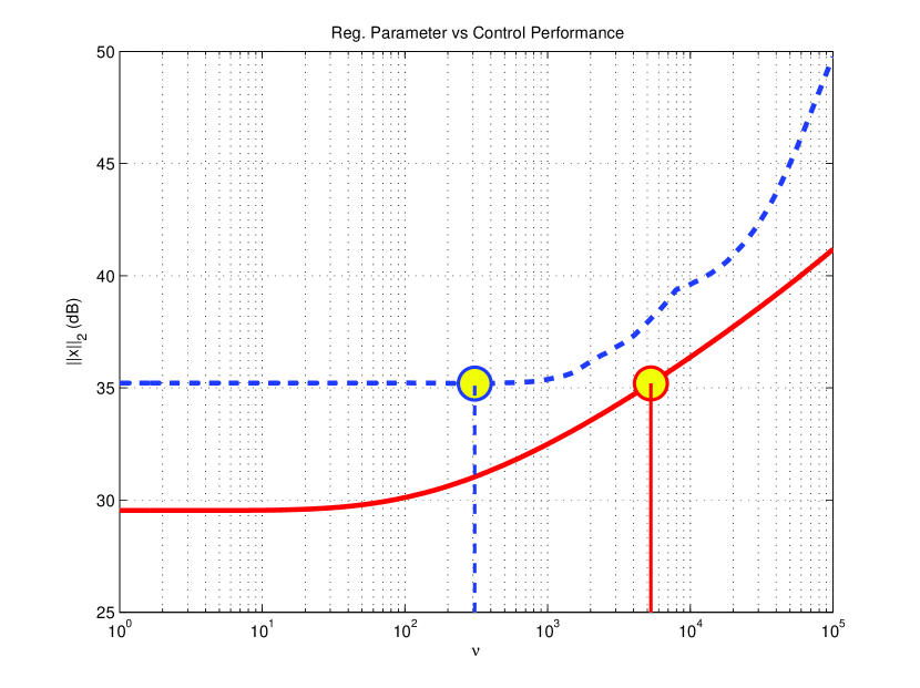
By this figure, we first find the optimal parameter for $\nu_{2}>0$ that optimizes the control performance, i.e., $\nu_{2}=3.1\times 10^{2}$. Then, we seek $\nu_{1}$ that gives the same control performance, namely, $\nu_{1}=5.3\times 10^{3}$. Furthermore, we also investigate the ideal least-squares solution ${\boldsymbol{u}}^{\star}({\boldsymbol{x}})$ that minimizes $\|G{\boldsymbol{u}}-H{\boldsymbol{x}}\|_{2}$.

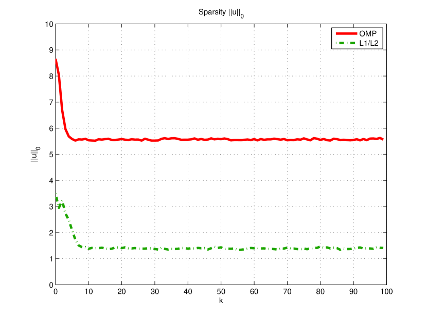
With these parameters, we run 500 simulations with randomly generated (Markovian) packet-dropouts that satisfy Assumption 4.1, and with initial vector ${\boldsymbol{x}}_{0}$ in which each element is independently sampled from the normal distribution with mean 0 and variance 1. Fig. 3 shows the averaged sparsity of the obtained control vectors.

Figure 3: Sparsity of the control vectors by ideal (star), $\ell^{2}$ with regularization parameter $\nu_{2}=3.1\times 10^{2}$, OMP (solid), $\ell^{1}/\ell^{2}$ with $\nu_{1}=5.3\times 10^{3}$ (dash-dot) and $\nu_{1}=5.3$ (dash).

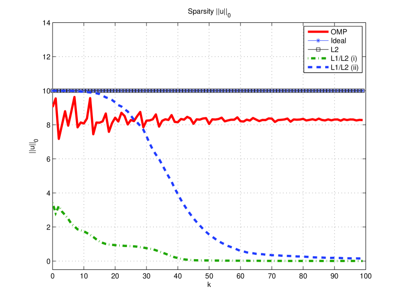
The $\ell^{1}/\ell^{2}$ optimization with $\nu_{1}=5.3\times 10^{3}$ always produces much sparser control vectors than those by OMP. This property depends on how to choose the regularization parameter $\nu_{1}>0$. In fact, if we choose smaller $\nu_{1}=5.3$, the sparsity changes as shown in Fig. 3. On the other hand, if we use a sufficiently large $\nu_{1}>0$, then the control vector becomes ${\boldsymbol{0}}$. This is indeed the sparsest control, but leads to very poor control performance: the state diverges until the control vector becomes nonzero (see [19]).

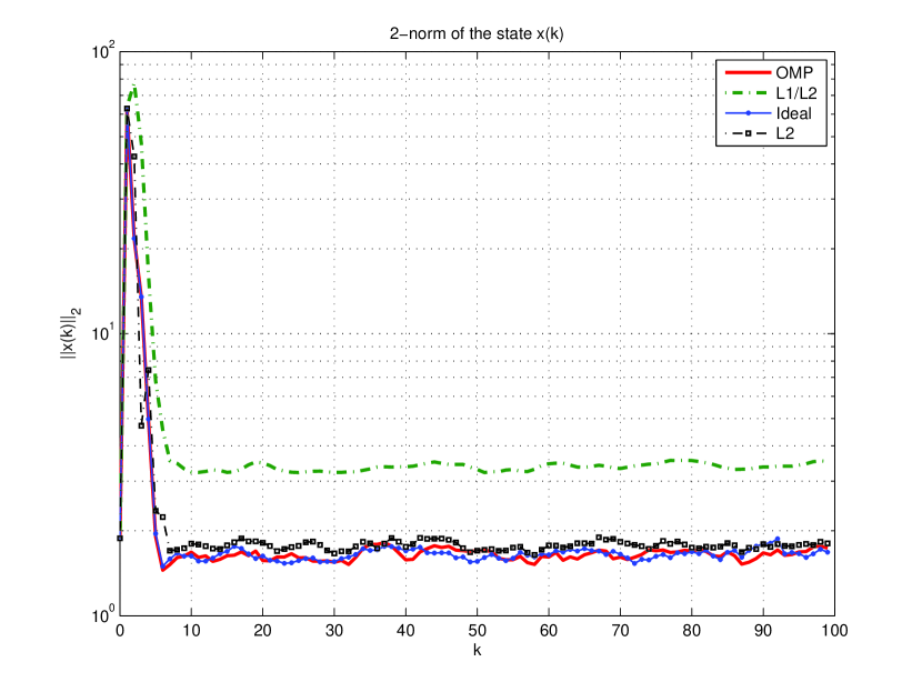
Fig. 4 shows the averaged 2-norm of the state ${\boldsymbol{x}}(k)$ as a function of $k$ for all 5 designs. We see that, with exception of the $\ell^{1}/\ell^{2}$ optimization based PPC, the NCSs are nearly exponentially stable. In contrast, if the $\ell^{1}/\ell^{2}$ optimization of[19] is used, then only practical stability is observed. The simulation results are consistent with Corollary 5.1 and our previous results in[19]. Note that the $\ell^{1}/\ell^{2}$ optimization with $\nu_{1}=5.3$ shows better performance than that with $\nu_{1}=5.3\times 10^{3}$, while $\nu_{1}=5.3\times 10^{3}$ gives a much sparser vector. This shows a tradeoff between the performance and the sparsity.

Figure 4: 2-norm of the state ${\boldsymbol{x}}(k)$ for the four PPC designs: log plot (above) and linear plot (below).

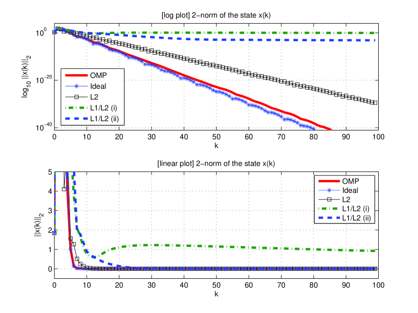
Fig. 5 shows the associated computation times.

Figure 5: Computational time.

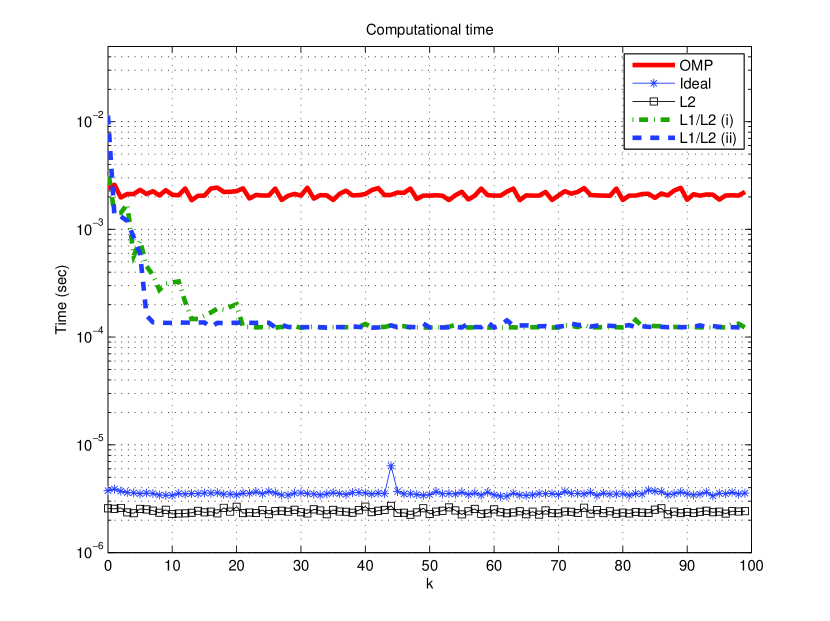
The $\ell^{1}/\ell^{2}$ optimization is faster than OMP in many cases. Note that the ideal and the $\ell^{2}$ optimizations are much faster, since they require just one matrix-vector multiplication.

6.2 Bit-rate Issues

We next investigate bit-rate aspects for a Gaussian plant noise process ${\boldsymbol{v}}(k)$. To keep the encoder and decoder simple, we will be using memoryless entropy-constrained uniform scalar quantization; see [30]. Thus, the non-zero elements of the control vector are independently encoded using a scalar uniform quantizer followed by a scalar entropy coder. In the simulations, we choose the step size of the quantizer to be $\Delta=0.001$, which results in negligible quantization distortion. We first run 1000 simulations with 100 time steps and use the obtained control vectors for designing entropy coders. A separate entropy coder is designed for each element in the control vector. For the first $N/2$ elements in the vector, we always use a quantizer followed by entropy coding. For the remaining $N/2$ elements, we only quantize and entropy code the non-zero elements. We then send additional $N/2$ bits indicating, which of the $N/2$ elements have been encoded. The total bit-rate for each control vector is obtained as the sum of the codeword lengths for each individual non-zero codeword $+N/2$ bits. For comparison, we use the same scalar quantizer with step size $\Delta=0.001$ and design entropy coders on the data obtained from the $\ell^{2}$ optimization. Since the control vectors in this case are non-sparse, we separately encode all $N$ elements and sum the lengths of the individual codewords to obtain the total bit-rate. In both of the above cases, the entropy coders are Huffman coders. Moreover, the system parameters are initialized with different random seeds for the training and test situations, respectively. The average rate per control vector for the OMP case is $55.36$ bits, whereas the average rate for the $\ell^{2}$ case is $112.57$ bits. Thus, due to sparsity, a $50.8$ percent bit-rate reduction is on average achieved.

Figure 6: 2-norm of the state ${\boldsymbol{x}}(k)$ with Gaussian noise.

Figure 7: Sparsity of the control vectors with Gaussian noise.

Fig. 6 shows the 2-norm of the state ${\boldsymbol{x}}(k)$ and Fig. 7 shows the sparsity. We can also see the tradeoff between the performance and the sparsity in this case.

7 Conclusion

We have studied a packetized predictive control formulation with a sparsity-promoting cost function for error-prone rate-limited networked control system. We have given sufficient conditions for asymptotic stability when the controller is used over a network with bounded packet dropouts. Simulation results indicate that the proposed controller provides sparse control packets, thereby giving bit-rate reductions when compared to the use of, more common, quadratic cost functions. Future work may include further study of performance aspects and the effect of plant disturbances.

References

- [1] W. Zhang, M. Branicky, and S. Phillips, “Stability of networked control systems,” IEEE Control Syst. Mag., vol. 21, pp. 84–99, Feb. 2001.
- [2] J. Hespanha, P. Naghshtabrizi, and Y. Xu, “A survey of recent results in networked control systems,” Proc. IEEE, vol. 95, pp. 138–162, Jan. 2007.
- [3] A. Bemporad, M. Heemels, and M. Johansson, Networked Control Systems. Springer, Oct. 2010.
- [4] A. Bemporad, “Predictive control of teleoperated constrained systems with unbounded communication delays,” Proc. IEEE CDC, pp. 2133–2138, 1998.
- [5] A. Casavola, E. Mosca, and M. Papini, “Predictive teleoperation of constrained dynamic systems via internet-like channels,” IEEE Trans. Control Syst. Technol., vol. 14, no. 4, pp. 681–694, 2006.
- [6] P. L. Tang and C. W. de Silva, “Stability validation of a constrained model predictive networked control system with future input buffering,” Int. J. Contr., vol. 80, no. 12, pp. 1954–1970, 2007.
- [7] D. Muñoz de la Peña and P. D. Christofides, “Lyapunov-based model predictive control of nonlinear systems subject to data losses,” IEEE Trans. Autom. Control, vol. 53, pp. 2076–2089, Sept. 2008.
- [8] D. E. Quevedo and D. Nešić, “Input-to-state stability of packetized predictive control over unreliable networks affected by packet-dropouts,” IEEE Trans. Autom. Control, vol. 56, pp. 370–375, Feb. 2011.
- [9] D. E. Quevedo, J. Østergaard, and D. Nešić, “Packetized predictive control of stochastic systems over bit-rate limited channels with packet loss,” IEEE Trans. Autom. Control, vol. 56, pp. 2854–2868, Dec. 2011.
- [10] G. Pin and T. Parisini, “Networked predictive control of uncertain constrained nonlinear systems: Recursive feasibility and input-to-state stability analysis,” IEEE Trans. Autom. Control, vol. 56, pp. 72–87, Jan. 2011.
- [11] D. L. Donoho, “Compressed sensing,” IEEE Trans. Inf. Theory, vol. 52, pp. 1289–1306, Apr. 2006.
- [12] E. J. Candes, “Compressive sampling,” Proc. International Congress of Mathematicians, vol. 3, pp. 1433–1452, Aug. 2006.
- [13] E. J. Candes and M. B. Wakin, “An introduction to compressive sampling,” IEEE Signal Process. Mag., vol. 25, pp. 21–30, Mar. 2008.
- [14] S. Mallat, A Wavelet Tour of Signal Processing. Elsevier, 2009.
- [15] M. Elad, Sparse and Redundant Representations. Springer, 2010.
- [16] J.-L. Starck, F. Murtagh, and J. M. Fadili, Sparse Image and Signal Processing. Cambridge University Press, 2010.
- [17] B. K. Natarajan, “Sparse approximate solutions to linear systems,” SIAM J. Comput., vol. 24, no. 2, pp. 227–234, 1995.
- [18] G. K. Wallace, “The JPEG still picture compression standard,” Commun. ACM, vol. 34, pp. 30–44, Apr. 1991.
- [19] M. Nagahara and D. E. Quevedo, “Sparse representations for packetized predictive networked control,” in IFAC 18th World Congress, pp. 84–89, Aug. 2011.
- [20] S. G. Mallat and Z. Zhang, “Matching pursuits with time-frequency dictionaries,” IEEE Trans. Signal Process., vol. 41, pp. 3397–3415, Nov. 1993.
- [21] Y. C. Pati, R. Rezaiifar, and P. S. Krishnaprasad, “Orthogonal matching pursuit: Recursive function approximation with applications to wavelet decomposition,” in Proc. the 27th Annual Asilomar Conf. on Signals, Systems and Computers, pp. 40–44, Nov. 1993.
- [22] M. Nagahara, D. E. Quevedo, and J. Østergaard, “Sparsely-packetized predictive control by orthogonal matching pursuit (extended abstract),” in 20th International Symposium on Mathematical Theory of Networks and Systems (MTNS), July 2012. to be presented.
- [23] S. Bhattacharya and T. Başar, “Sparsity based feedback design: a new paradigm in opportunistic sensing,” in Proc. of American Control Conference, pp. 3704–3709, Jul. 2011.
- [24] M. Nagahara, D. E. Quevedo, T. Matsuda, and K. Hayashi, “Compressive sampling for networked feedback control,” in Proc. IEEE Int. Conf. Acoust. Speech Signal Process (ICASSP), pp. 2733–2736, Mar. 2012.
- [25] D. E. Quevedo, J. Østergaard, and D. Nešić, “Packetized predictive control of stochastic systems over bit-rate limited channels with packet loss,” IEEE Trans. Autom. Control, vol. 56, no. 11, 2011.
- [26] A. M. Bruckstein, D. L. Donoho, and M. Elad, “From sparse solutions of systems of equations to sparse modeling of signals and images,” SIAM Rev., vol. 51, pp. 34–81, Feb. 2009.
- [27] P. Massioni, F. Ankersen, and M. Verhaegen, “A matching pursuit algorithm approach to chaser-target formation flying problems,” IEEE Trans. Control Syst. Technol., 2011. (to appear).
- [28] D. Bertsimas and A. Thiele, “A robust optimization approach to inventory theory,” Operations Research, vol. 54, pp. 150–168, Jan.–Jeb. 2006.
- [29] J. M. Maciejowski, Predictive Control with Constraints. Prentice-Hall, 2002.
- [30] T. M. Cover and J. A. Thomas, Elements of Information Theory. Wiley–Interscience, 2nd ed., 2006.