Rayleigh-Ritz variational method with suitable asymptotic behaviour

Abstract

We discuss Rayleigh-Ritz variational calculations with nonorthogonal basis sets that exhibit the correct asymptotic behaviour. We construct the suitable basis sets for general one-dimensional models and illustrate the application of the approach on two double-well oscillators proposed recently by other authors. The rate of convergence of the variational method proves to be considerably greater than the one exhibited by the recently developed orthogonal polynomial projection quantization.

1 Introduction

In a recent paper Handy and Vrinceanu[1] proposed a method for the calculation of energy eigenvalues that is based on the projection of the bound-state wavefunction onto sets of orthogonal polynomials. The approach named orthogonal polynomial projection quantization (OPPQ) proved to be rapidly converging and more stable than the Hill determinant methods.

Among other models the authors considered the sextic $V_{S}(x)=x^{6}-4x^{2}$ and quartic $V_{Q}(x)=x^{4}-5x^{2}$ two-well oscillators. The bound states behave asymptotically as $\psi(x)\sim e^{-x^{4}/4}$ and $\psi(x)\sim e^{-|x|^{3}/3}$ in the former and latter case, respectively. Handy and Vrinceanu[1] chose the reference functions $R_{G}(x)=e^{-x^{2}/2}$ and $R_{TT}(x)=e^{-x^{4}/4}$ and showed that the latter is preferable for $V_{S}(x)$ while the former is more convenient for $V_{Q}(x)$. In fact, $R_{TT}(x)$ exhibits the correct asymptotic behaviour for the potential $V_{S}(x)$. At first sight it appears to be surprising that the authors did not try the reference function $R(x)=e^{-|x|^{3}/3}$, which is expected to be suitable for the quartic double well, since their approach permits the use of arbitrary nonanalytic positive reference functions[1].

The purpose of this paper is to show that it is quite straightforward to apply the variational Rayleigh-Ritz method (RRM) with a basis set that exhibits the correct asymptotic behaviour of the eigenfunctions for the models discussed above. In addition to it, we deem it worthwhile to compare the well known, extremely reliable and widely used RRM with the recently developed OPPQ.

In section 2 we develop the basis sets with suitable asymptotic behaviours for some general one-dimensional models. In section 3 we calculate the eigenvalues for the oscillators $V_{S}(x)$ and $V_{Q}(x)$ with three basis sets having different asymptotic behaviours, including the correct one for each model. We also compare RRM and OPPQ results for two models and two basis sets. Finally, in section 4 we summarize the main conclusions of the paper.

2 Basis functions with suitable asymptotic behaviour

In this section we show how to build a non-orthogonal basis set with the appropriate asymptotic behaviour at infinity. To this end we generalize a procedure proposed recently by Fernández[2] for a particular case. For simplicity we focus on the one-dimensional eigenvalue equation

$$-\psi^{\prime\prime}(x)+V(x)\psi(x)=E\psi(x),$$ (1)

and assume tat

$$\lim\limits_{|x|\rightarrow\infty}x^{-2k}V(x)=a>0.$$ (2)

Under such condition the eigenfunctions behaves asymptotically as

$$\psi(x) \sim e^{-|S_{k}(x)|}$$

$$S_{k}(x) = \frac{\sqrt{a}}{k+1}x^{k+1}.$$ (3)

We consider the following cases:

Case 1: Parity-invariant potential $V(-x)=V(x)$.

a) $k$ even. The non-orthogonal basis set is of the form

$$f_{j}(x) = |x|^{j}e^{-|S_{k}(x)|},\,j=0,2,3,\ldots\mathrm{\ even\,states},$$

$$f_{j}(x) = x|x|^{j}e^{-|S_{k}(x)|},\,j=0,1,\ldots\mathrm{\ odd\,states},$$ (4)

b) $k$ odd. In this case we choose

$$f_{j}(x) = x^{2j+s}e^{-S_{k}(x)},\,j=0,1,\ldots$$

$$s = \left\{\begin{array}[]{c}0\mathrm{\ }\mathrm{even\,states}\\ 1\mathrm{\ }\mathrm{odd\,states}\end{array}\right..$$ (7)

Case 2: Asymmetric potential $V(-x)\neq V(x)$. The basis set is

$$f_{j}(x)=x^{j}e^{-|S_{k}(x)|},\,j=0,1,\ldots$$ (8)

For concreteness in what follows we consider two of the examples discussed by Handy and Vrinceanu[1]

$$V_{Q}(x)=x^{4}-5x^{2},$$ (9)

and

$$V_{S}(x)=x^{6}-4x^{2},$$ (10)

with asymptotic behaviours given by $S_{2}(x)=x^{3}/3$ and $S_{3}(x)=x^{4}/4$, respectively. However, they chose reference functions associated to $S_{3}(x)$ and $S_{1}(x)=x^{2}/2$ for the two models.

The RRM enables us to obtain the eigenvalues approximately from the roots of the secular determinant

$$\left|\mathbf{H}-E\mathbf{S}\right|=0,$$ (11)

where $\mathbf{H}$ and $\mathbf{S}$ are $N\times N$ square matrices with elements

$$H_{ij}=\left\langle f_{i}\right|\hat{H}\left|f_{j}\right\rangle,\,S_{ij}=\left\langle f_{i}\right|\left.f_{j}\right\rangle,$$ (12)

and $\hat{H}=\hat{p}^{2}+V(x)$. Once we have the approximate eigenvalues we obtain the eigenvectors from the secular equation

$$\left(\mathbf{H}-E\mathbf{S}\right)\mathbf{C=0,}$$ (13)

where $\mathbf{C}$ is an $N\times 1$ column matrix with the coefficients $c_{j}$ of the variational trial function.

The application of this approach to the Schrödinger equation with a parity-invariant potential is particularly simple because we can restrict the calculation of the matrix elements to the half line $x>0$[2]. Since all the matrix elements reduce to integrals of the form

$$\left\langle f\right|\left.g\right\rangle=\int_{0}^{\infty}f(x)g(x)\,dx,$$ (14)

then we do not have to take into account the absolute value of the coordinate explicitly when $k$ is even.

3 Results

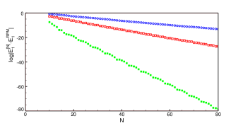
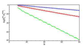
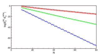
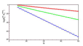
We first verify the effect of the asymptotic behaviour of the basis sets (4) and (7) on the rate of convergence of the RRM. A reasonable estimate of the rate of convergence is the logarithmic error $L_{N}=\log\left|E_{n}^{(app)}-E_{n}^{(RPM)}\right|$ where $E_{n}^{(app)}$ is the eigenvalue calculated by any of the methods described in this paper and $E_{n}^{(RPM)}$ is a very accurate result obtained by means of the RPM[3, 4]. Figure 1 shows $L_{N}$ for the first four eigenvalues of (9) calculated by means of the RRM with the functions $S_{1}(x)$, $S_{2}(x)$ and $S_{3}(x)$ in terms of the number of basis functions $N$. We see that the rate of convergence decreases according to $S_{2}(x)>S_{1}(x)>S_{3}(x)$; that is to say, the RRM converges more rapidly when choosing the correct asymptotic behaviour $S_{2}(x)$. On the other hand, figure 2 shows that the relative rate of convergence of the RRM for the potential (10) is $S_{3}(x)>S_{2}(x)>S_{1}(x)$. Once again the greater rate of convergence is given by the correct asymptotic behaviour $S_{3}(x)$. Besides, the second inequality appears to be reasonable because $S_{2}(x)$ is closer to the correct asymptotic behaviour than $S_{1}(x)$.

We think that it is also worthwhile to compare the rate of convergence of the simple, well known and reliable RRM and the rather more elaborate OPPQ using the same basis set in both approaches. Handy and Vrinceanu[1] chose the reference function $R_{G}(x)=e^{-x^{2}/2}$ for the PT-symmetric potential

$$V(x)=ix^{3}$$ (15)

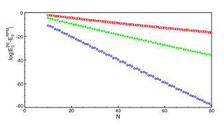
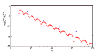
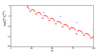
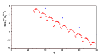
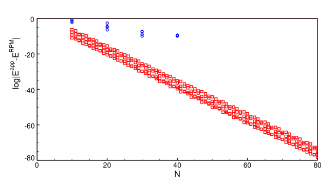
and we therefore choose the function $S_{1}(x)$ for the RRM. More precisely, instead of the non-orthogonal basis set (7) we resorted to the eigenfunctions of the harmonic oscillator that are truly consistent with the orthogonal Hermite polynomials used by those authors. Figure 3 shows $L_{N}$ for the first four eigenvalues calculated by both methods. It clearly shows that the RRM rate of convergence is noticeably greater that the OPPQ one.

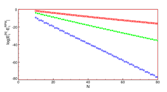
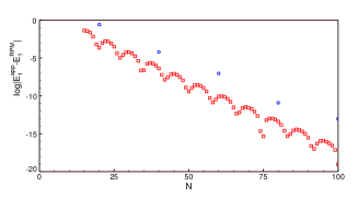
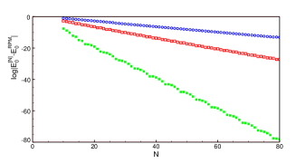
The better performance of the RRM is not restricted to the PT-symmetric cubic oscillator; this approach converges more rapidly for the two other models discussed above. For example, figure 4 compares the logarithmic errors of both approaches for the eigenvalues of the double-well oscillator (10). In this case we have chosen the basis set with the correct asymptotic behaviour $S_{3}(x)$ for the RRM and the OPPQ results for $R_{TT}(x)=e^{-x^{4}/4}$[1]. The difference between the convergence rates of both approaches is even more dramatic for this oscillator. However, it makes more sense for small $N$ because the number of significant digits of the OPPQ results reported by the authors is rather small for a fair comparison at large $N$.

Finally, we deem it worthwhile to show the RPM eigenvalues chosen as a reference for the calculation of the logarithmic errors. We have

$$E_{0} = -3.41014276123982947529770965352190919871233904756$$

$$4881868937911775329611301715294$$

$$E_{1} = -3.250675362289235980228513775547736877154601147639$$

$$4241429953014335680690809034749688022953825298$$

$$E_{2} = 0.6389195637838381244910101033325042648524013290581$$

$$37207433367771840730088316019330941500824$$

$$E_{3} = 2.5812162706174514809779380656962090234197947974759$$ (16)

$$598949291704975284539346710703866627200928172$$

for (9)

$$E_{0} = -0.5232686221275522394161694971907840611656342225187$$

$$11069953854385633821213450649003542309$$

$$E_{1} = 1.00576834022554481670604083074777604686886504417542$$

$$730471341100873617568288708176003637$$

$$E_{2} = 5.37497000884004499406051476941823532582175431150133$$

$$8177585996687355671683247232390293$$

$$E_{3} = 10.5725850445859121139060615553140114648422138800575$$ (17)

$$29217715660995992776130576146017312$$

for (10) and

$$E_{0} = 1.156267071988113293799219177999951$$

$$E_{1} = 4.1092287528096515358436684785613$$

$$E_{2} = 7.5622738549788280413518091106314827208$$

$$E_{3} = 11.314421820195804402233783948426989$$ (18)

for (15). These quite accurate results may be used as benchmarks for other approaches.

4 Conclusions

We have shown that it is not difficult to introduce the correct asymptotic behaviour of the wavefunction into the RRM variational trial function, specially if the potential is parity invariant. Present results clearly show that the correct asymptotic behaviour increases the rate of convergence of the approach dramatically. In principle, the same strategy can be implemented through the appropriate OPPQ reference function but it has not yet been tried for the case of $k$ even[1].

We have also shown that the rate of convergence of the RRM is considerably greater than that for the OPPQ. In addition to it the former approach is simpler and more straightforward. The integrals that appear in both approaches are basically the same and can in principle be calculated by the same algorithms. Here we just compared the results for two oscillators and two basis sets with different asymptotic behaviours but the trend is exactly the same for the other possible combinations of model and basis set.

We do not know the reason why the RRM rate of convergence is so much greater than the OPPQ one. What we already know is that in the case of the Hermitian Hamiltonians the former approach exhibits the additional advantage that its approximate eigenvalues tend to the exact ones from above. On the other hand, the OPPQ eigenvalues do not appear to exhibit any bounding property.

Figure 1: Logarithmic errors for the first four eigenvalues of the double well $V_{Q}(x)$ calculated by means of the basis sets with $S_{1}(x)$ (squares, red) $S_{2}(x)$ (filled squares, green) and $S_{3}(x)$ (circles, blue)

Figure 2: Logarithmic errors for the first four eigenvalues of the double well $V_{S}(x)$ calculated by means of the basis sets with $S_{1}(x)$ (squares, red) $S_{2}(x)$ (filled squares, green) and $S_{3}(x)$ (circles, blue)

Figure 3: Logarithmic errors for the first four eigenvalues of the PT-symmetric potential (15) calculated by means of the RRM (squares, red) and the OPPQ method (circles, blue)

Figure 4: Logarithmic errors for the first four eigenvalues of the double well $V_{S}(x)$ calculated by means of the RRM (squares, red) and the OPPQ method (circles, blue)

References

• [1] Handy C N and Vrinceanu D 2013 J. Phys. A 46 135202.
• [2] Fernández 2013 Cent. Eur. J. Phys. (in the press), arXiv:1204.0229 [math-ph].
• [3] Fernández F M, Ma Q, and Tipping R H 1989 Phys. Rev. A 39 1605.
• [4] Fernández F M, Ma Q, and Tipping R H 1989 Phys. Rev. A 40 6149.
Refer to caption