Some Quantitative Results in Real Algebraic Geometry

Abstract

Real algebraic geometry is the study of semi-algebraic sets, subsets of $\textnormal{{R}}^{k}$ defined by boolean combinations of polynomial equalities and inequalities. The focus of this thesis is to study quantitative results in real algebraic geometry, primarily upper bounds on the topological complexity of semi-algebraic sets as measured, for example, by their Betti numbers. Another quantitative measure of topological complexity which we study is the number of homotopy types of semi-algebraic sets of bounded description complexity. The description complexity of a semi-algebraic set depends on the context, but it is simply some measure of the complexity of the polynomials in the formula defining the semi-algebraic set (e.g., the degree and number of variables of a polynomial, the so called dense format). We also provide a description of the Hausdorff limit of a one-parameter family of semi-algebraic sets, up to homotopy type which the author hopes will find further use in the future. Finally, in the last chapter of this thesis, we prove a decomposition theorem similar to the well-known cylindrical decomposition for semi-algebraic sets but which has the advantage of requiring significantly less cells in the decomposition. The setting of this last result is not in semi-algebraic geometry, but in the more general setting of o-minimal structures.

Barone, Salvador Doctor of PhilosophyPh.D.August2013 Saugata Basu West Lafayette

Chapter 1 Preliminaries

In this chapter we provide some background theory for the results of Chapter 2 and Chapter 3. The content of Chapter 4 is self-contained except for the definition of real closed fields (Definition I.1).

I Real closed fields and extensions

We first define real closed fields and list some of their important properties. A field R is an ordered field if it is totally ordered and the order is compatible with the field operations, namely, for every $a,b,c\in\textnormal{{R}}$ we have

$$a\leq b \implies a+c\leq b+c,\text{ and}$$

$$a\geq 0\wedge b\geq 0 \implies ab\geq 0.$$

Definition I.1.

An ordered field R is real closed if R has no algebraic ordered extensions.

There are several equivalent definitions for a field to be real closed (see BPRbook2 ).

Theorem I.2 (Theorem 2.11 BPRbook2 ).

Let R be a field. Then the following are equivalent:

• R is real closed.

• $\textnormal{{R}}[i]=\textnormal{{R}}[T]/(T^{2}+1)$ is an algebraically closed field.

• R has the intermediate value property.

• The non-negative elements of R are exactly squares of the form $a^{2}$, and every polynomial in $\textnormal{{R}}[X]$ of odd degree has a root in R.

The prototypical example of a real closed field is $\mathbb{R}$ the field of real numbers. However, the use of an arbitrary real closed field as a base field is pervasive in real algebraic geometry. The reason for working over an arbitrary real closed field rather than $\mathbb{R}$ is two-fold. First, for mathematical reasons it is desirable to prove results using the smallest number of assumptions as possible in order to make the results stronger. More importantly is the fact that in the proof of many results it is extremely useful to consider ordered field extensions of the starting base field and thus it is useful for theorems to hold over arbitrary real closed fields (see Section I.1).

I.1 Real extensions, algebraic Puiseux series

For any R ordered field, a real extension of R is an ordered field $\textnormal{{R}}^{\prime}$ such that $\textnormal{{R}}\subseteq\textnormal{{R}}^{\prime}$ and the ordering of $\textnormal{{R}}^{\prime}$ restricted to R is just the order on R (note that if R is real closed this implies that the extension is not algebraic). One of the main tools we will use is a certain type of real extension, namely, the extension of a real closed field by an infinitesimal.

Let R be a real closed field. A Puiseux series with coefficients in R is a formal Laurent series in the indeterminate $\varepsilon^{1/q}$, which takes the form $\sum_{i\geq k}a_{i}\varepsilon^{i/q}$, $i\in\mathbb{Z}$, $a_{i}\in\textnormal{{R}}$, and $q$ a positive integer. Under the ordering $0<\varepsilon<a$ for any $a\in\textnormal{{R}}$, the field of Puiseux series is real closed extension of R (see BPRbook2 ) in which $\varepsilon$ is an infinitesimal. We will primarily be concerned with the real closed subfield $\textnormal{{R}}\langle\varepsilon\rangle$ of algebraic Puiseux series, those Puiseux series which are algebraic over $\textnormal{{R}}(\varepsilon)$.

An important concept regarding algebraic Puiseux series which will be discussed in greater detail in Chapter 2 (Section II.5) is the notion of limits. A Puiseux series $\xi$ is bounded over R if $|\xi|<a$ for some $a\in\textnormal{{R}}$. We denote the set of Puiseux series bounded over R by $\textnormal{{R}}\langle\varepsilon\rangle_{b}$. We define the $\lim_{\varepsilon}$ map to be the ring homomorphism from $\textnormal{{R}}\langle\varepsilon\rangle_{b}$ to R which sends a Puiseux series $\sum_{i\geq 0}a_{i}\varepsilon^{i/q}$ to $a_{0}$. The map $\lim_{\varepsilon}$ simply replaces $\varepsilon$ by $0$ in a Puiseux series which has no terms corresponding to negative indices.

II Semi-algebraic sets and formulas

We now formally define semi-algebraic sets, using the definition found in BPRbook2 . The semi-algebraic sets of $\textnormal{{R}}^{k}$ are the smallest collection of subsets of $\textnormal{{R}}^{k}$ defined by polynomial equalities or polynomial strict inequalites, i.e., sets of the form $\{x\in\textnormal{{R}}^{k}|\;P(x)=0\}$ or $\{x\in\textnormal{{R}}^{k}|\;P(x)>0\}$ respectively, which is closed under the boolean operations (finite intersections, finite unions, and taking complements). Semi-algebraic sets can be described by formulas involving polynomial equalities and inequalities, and to make this precise we next define what we mean by a formula.

In the language of logic, a quantifier-free formula is defined inductively: an atom is a quantifier-free formula, and if $\alpha,\beta$ are two quantifier-free formulas then $\alpha\wedge\beta$, $\alpha\vee\beta$, and $\neg\alpha$ are quantifier-free formulas. All of the variables in a quantifier-free formula are called free variables. In the case of semi-algebraic sets, the atoms are polynomial equalities $P=0$ and strict inequalites $P>0$, where $P\in\textnormal{{R}}[X_{1},\ldots,X_{k}]$, and the free variables are $X_{1},\ldots,X_{k}$. The free variables of a formula can be quantified by either the existential quantifier $\exists X_{i}$ or the universal quantifier $\forall X_{i}$, and a free variable once quantified is no longer free but a bound variable.

Using elementary logic, it is clear that any formula can be expressed using only the unary connective $\neg$, the binary connective $\wedge$, and the existential quantifier $\exists$. These logical symbols have a corresponding meaning in the geometry of semi-algebraic sets, namely the set theoretic operations of complement, intersection, and projection, respectively. For example,

$$\{x\in\textnormal{{R}}^{k}|\;P(x)\neq 0\}=\textnormal{{R}}^{k}\smallsetminus\{x\in\textnormal{{R}}^{k}|\;P(x)=0\},$$

$$\{x\in\textnormal{{R}}^{k}|\;P(x)>0\wedge Q(x)=0\}=\{x\in\textnormal{{R}}^{k}|\;P(x)>0\}\cap\{x\in\textnormal{{R}}^{k}|\;Q(x)=0\},$$

and

$$\{x^{\prime}\in\textnormal{{R}}^{k-1}|\;(\exists X_{k})P(x^{\prime},X_{k})=0\}=\pi(\{x\in\textnormal{{R}}^{k}|\;P(x)=0\}),$$

where $\pi:\textnormal{{R}}^{k}\to\textnormal{{R}}^{k-1}$ is the projection which forgets the last coordinate. It is an important consequence of the Tarski-Seidenberg Theorem that when R is real closed that the projection of a semi-algebraic set in $\textnormal{{R}}^{k}$ is again semi-algebraic. Said another way, any formula defined over R with quantifiers is equivalent to a quantifier-free formula in the free variables. So, any formula where the atoms are polynomial equalities and inequalities over a real closed field defines a semi-algebraic set.

One important type of semi-algebraic set are the basic semi-algebraic sets. Let R be a real closed field and suppose $S$ is a semi-algebraic subset of $\textnormal{{R}}^{k}$ defined by a conjunction of equalities and strict inequalities of $k$-variate polynomials. Such a semi-algebraic set is called a basic semi-algebraic set. Since any quantifier-free formula can be put into disjunctive normal form, as a disjunction of conjunctions, any semi-algebraic set is the union of basic semi-algebraic sets. In symbols, any set of the form

$$\{x\in\textnormal{{R}}^{k}|\;P(x)=0\wedge\bigwedge_{Q\in\mathcal{Q}}Q(x)>0\}$$

is a basic semi-algebraic set, for $\mathcal{Q}$ a finite subset of $\textnormal{{R}}[X_{1},\ldots,X_{k}]$.

Although semi-algebraic sets are described by formulas, it is obvious that many formulas can define the same semi-algebraic set (try to think of several formulas that define the empty set). On the other hand, one formula can describe different semi-algebraic sets over different real closed fields if one considers field extensions. If $S$ is a semi-algebraic subset of $\textnormal{{R}}^{k}$ defined by $\phi$, and $\textnormal{{R}}\subseteq\textnormal{{R}}^{\prime}$ is a real closed extension, then $\text{Ext}(S,\textnormal{{R}}^{\prime})$ is the semi-algebraic subset of $\textnormal{{R}}^{\prime k}$ defined by $\phi$.

II.1 Tame geometry

Although it will not be relevant until Chapter 4, we take a moment to step back to discuss an important property which semi-algebraic geometry shares with other branches of real algebraic geometry: the property for a geometry to be tame. In a precise mathematical sense, the geometry of semi-algebraic sets is tame. Bizzare geometric phenomenon like the space filling curve or the topologists sin curve $y=\sin(1/x)$ can not occur in tame geometries. While many quantitative results (e.g., on the Betti numbers of semi-algebraic sets, homotopy types, etc.) do not have immediate analogues in other tame geometries, many results about semi-algebraic sets can be deduced as special cases of results which hold in all tame geometries.

In Chapter 4 we will prove a result in a more general framework than the theory of semi-algebraic sets. In particular, we will prove a result which holds over an arbitrary o-minimal structure (see Section I).

III Homotopy types, Betti numbers, and homology of semi-algebraic sets

In this section we provide the definitions which we will need in Chapters 2 and 3.

III.1 Homotopy types

We recall some definitions from BPRbook2 (Section 6.3). Let $X,Y$ be two closed and bounded semi-algebraic sets and $f,g:X\to Y$ two semi-algebraic functions (a function $f:X\to Y$ is semi-algebraic if its graph $\Gamma(f)=\{(x,y)|\;f(x)=y\}$ is a semi-algebraic subset of $X\times Y$). We say that $f$ and $g$ are semi-algebraically homotopic if there exists a semi-algebraic and continuous function $F:X\times[0,1]\to Y$ such that $F(x,0)=f(x)$ and $F(x,1)=g(x)$. If there exists semi-algebraic continuous maps $f:X\to Y$ and $g:Y\to X$ such that $f\circ g$ is semi-algebraically homotopic to the identity map of $Y$ and $f\circ g$ is semi-algebraically homotopic to the identity map of $X$, then we say that $X$ and $Y$ are semi-algebraically homotopy equivalent. It is clear that semi-algebraic homotopy equivalence is an equivalence relation. If $X\supseteq Y$ and there exists a semi-algebraic and continuous function $h:X\times[0,1]\to X$ such that $h(-,0)$ is the identity function of $X$ and $h(-,1)$ takes values in $Y$, then we say that $h$ is a deformation retract of $X$ to $Y$, and in this case it is clear (using techniques of elementary topology, see, e.g., munkres2000topology ) that $X$ and $Y$ are semi-algebraically homotopy equivalent.

III.2 Betti numbers of semi-algebraic sets

In this section we provide a brief introduction to the Betti numbers of semi-algebraic sets, see BPRbook2 for a detailed introduction. The definition for the Betti numbers of closed and bounded semi-algebraic set $S$ is to use the fact that any closed and semi-algebraic semi-algebraic set can be triangulated, it is homeomorphic to a simplicial complex, and then to define the homology groups of the semi-algebraic set $S$ as the simplicial homology groups of the associated simplicial complex $K$. For locally closed semi-algebraic sets, one defines the Betti numbers using Borel-Moore homology, which has the advantage of being additive and coincides with the simplicial complex definition of Betti numbers in the case of closed semi-algebraic sets. In order to be precise in this exposition we provide the following definitions which already appear in BPRbook2 (see in particular Sections 5.6 and 5.7, and Chapter 6).

Let $a_{0},\ldots,a_{d}$ be affinely independent points of $\textnormal{{R}}^{k}$, so that they are not contained in any $d-1$ dimensional affine subspace. The $d$-simplex with vertices $a_{0},\ldots,a_{d}$ is the set

$$\{\lambda_{0}a_{0}+\ldots+\lambda_{d}a_{d}|\;\sum_{i=0}^{d}\lambda_{i}=1\text{ and }\lambda_{0},\ldots,\lambda_{d}\geq 0\},$$

and an $e$-face of the $d$-simplex $[a_{0},\ldots,a_{d}]$ is any $e$-simplex $[b_{0},\ldots,b_{e}]$ such that

$$\{b_{0},\ldots,b_{e}\}\subseteq\{a_{0},\ldots,a_{d}\}.$$

A simplicial complex $K$ in $\textnormal{{R}}^{k}$ is a finite set of simplicies in $\textnormal{{R}}^{k}$ such that if $s,s^{\prime}\in K$ then every face of $s$ is in $K$ and $s\cap s^{\prime}$ is a common face of both $s$ and $s^{\prime}$.

It is proved in BPRbook2 (Theorem 5.43) that any closed and bounded semi-algebraic set can be triangulated.

Theorem III.1 (Theorem 5.43 BPRbook2 ).

Let $S\subseteq\textnormal{{R}}^{k}$ be a closed and bounded semi algebraic set. Then there exists a simplicial complex $K$ of $\textnormal{{R}}^{k}$ and a semi-algebraic homeomorphism $h:K\to S$, called the triangulation of $S$.

For a closed and bounded semi-algebraic set $S$ let $K$ be as in Theorem III.1. We define

$$b_{i}(S):=b_{i}(K)$$

where $b_{i}(K)$ is the rank of the simplicial homology group $H_{p}(K)$ as a finite vector space over $\mathbb{Q}$ (see, for example, BPRbook2 Section 6.1 for a detailed introduction to the homology of simplicial complexes) or sometimes taking $\mathbb{Z}$, $\mathbb{Z}_{2}$ instead as the ring of coefficients, depending on the context in which we are working. The number of connected components, the Euler characteristic, and the sum of the Betti numbers of $S$ are thus defined respectively as

$$b_{0}(S)$$ ,

$$\chi(S):= \sum_{i=0}^{k}(-1)^{i}b_{i}(S),$$

$$b(S):= \sum_{i=0}^{k}b_{i}(S).$$

For a semi-algebraic set $S$ which is closed but not necessarily bounded, we can use the conical structure at infinity of semi-algebraic sets to define the Betti numbers of $S$. The following corollary follows immediately from the semi-algebraic triviality theorem (see Chapter 5, Theorem I.12 for an o-minimal version of the triviality theorem and BPRbook2 for a proof of the corollary).

Notation III.2

For any $r\in\textnormal{{R}}$, we denote by $B_{k}(0,r)$ semi-algebraic subset of $\textnormal{{R}}^{k}$ defined by the inequality $x_{1}^{2}+\ldots+x_{k}^{2}\leq r^{2}$. We will slightly abuse notation at times and use this notation to refer also to the semi-algebraic subset of $\textnormal{{R}}^{\prime k}$ defined by the same inequality for other real closed fields $\textnormal{{R}}^{\prime}$ and $r\in\textnormal{{R}}^{\prime}$, and we hope that this does not cause any confusion.

Theorem III.3 (Corollary 5.49 BPRbook2 , Conic structure at infinity).

Let $S$ be a closed semi-algebraic subset of $\textnormal{{R}}^{k}$. Then, there exists $r\in\textnormal{{R}}$, $r>0$, such that for every $r^{\prime}\geq r$, there is a semi-algebraic deformation retraction from $S$ to $S_{r^{\prime}}=S\cap\overline{B_{k}(0,r^{\prime})}$ and a semi-algebraic deformation retraction from $S_{r^{\prime}}$ to $S_{r}$.

If $S$ is a closed semi-algebraic set then we define $b(S):=b(S\cap\overline{B_{k}(0,r)})$ for some sufficiently large $r$ satisfying the conclusion of Theorem III.3, which is well defined since homology is stable under semi-algebraic homotopy equivalence (Theorem 6.42 BPRbook2 ).

Finally, we define the Betti numbers of a certain type of semi-algebraic set which we next describe and which will be an important definition of Chapter 2. Let ${\mathcal{P}}$ be a finite subset of $\textnormal{{R}}[X_{1},\ldots,X_{k}]$. A sign condition on ${\mathcal{P}}$ is an element of $\{0,1,-1\}^{\mathcal{P}}$.

The realization of the sign condition $\sigma$ in a semi-algebraic set $V\subset\textnormal{{R}}^{k}$ is the semi-algebraic set

$${\mathcal{R}}(\sigma,V)=\{x\in V\;\mid\;\bigwedge_{P\in{\mathcal{P}}}\textrm{ sign}({P}(x))=\sigma(P)\}.$$ (III.1)

We define the Betti numbers of (the realization of) sign conditions as follows (following Section 6.3 of BPRbook2 ). Consider the field $\textnormal{{R}}\langle\delta\rangle$ of algebraic Puiseux series in $\delta$, and let $\overline{{\rm Reali}}(\sigma)$ be the semi-algebraic subset of $\textnormal{{R}}\langle\delta\rangle^{k}$ defined by

$$\sum_{1\leq i\leq k}X^{2}_{i}\leq 1/\delta\wedge\bigwedge_{\sigma(P)=0}P=0\wedge\bigwedge_{\sigma(P)=-1}P\leq-\delta\wedge\bigwedge_{\sigma(P)=1}P\geq\delta.$$

Note that $\overline{{\rm Reali}}(\sigma)$ is closed and bounded. As in BPRbook2 , we define $b({\rm Reali}(\sigma)):=b(\overline{{\rm Reali}}(\sigma))$, which is a good definition since the set $\overline{{\rm Reali}}(\sigma)$ is a semi-algebraic deformation retraction of the extension of ${\rm Reali}(\sigma)$ to $\textnormal{{R}}\langle\delta\rangle$ (Proposition 6.45 BPRbook2 ) and the homology of closed and bounded semi-algebraic sets is invariant under homotopy equivalence (Theorem 6.42 BPRbook2 ) and furthermore the homology groups of $S$ and those of its extension to a bigger real closed field are isomorphic. For an excellent and concise exposition of homology of sign conditions and semi-algebraic sets, see BPR8 .

IV CW complexes

We will need a few facts from the homotopy theory of finite CW-complexes in Chapter 3.

We first prove a basic result about $p$-equivalences (Definition I.2). It is clear that $p$-equivalence is not an equivalence relation (e.g., for any $p\geq 0$, the map taking $\mbox{${\bf S}$}^{p}$ to a point is a $p$-equivalence, but no map from a point into $\mbox{${\bf S}$}^{p}$ is one). However, we have the following.

Proposition IV.1.

Let $A,B,C$ be finite CW-complexes with $\dim(A),\dim(B)\leq k$ and suppose that $C$ is $p$-equivalent to $A$ and $B$ for some $p>k$. Then, $A$ and $B$ are homotopy equivalent.

The proof of Proposition IV.1 will rely on the following well-known lemmas.

Lemma IV.2.

(Whitehead, , page 182, Theorem 7.16) Let $X,Y$ be CW-complexes and $f:X\rightarrow Y$ a $p$-equivalence. Then, for each CW-complex $M$, $\dim(M)\leq p$, the induced map

$$f_{*}:[M,X]\rightarrow[M,Y]$$

is surjective.

Lemma IV.3.

(Viro-homotopy, , page 69) If $A$ and $B$ are finite CW-complexes, with $dim(A)<p$ and $dim(B)\leq p$, then every $p$-equivalence from $A$ to $B$ is a homotopy equivalence.

Proof IV.4 (Proof of Proposition IV.1).

See Barone-Basu11b .

Chapter 2 Refined bounds

In this chapter we prove that the number of semi-algebraically connected components of sign conditions on a variety is bounded singly exponentially in terms of the degree of the polynomials defining the sign condition, the degree of the polynomials defining the variety, the dimension of the variety, and the dimension of the ambient space.

Let R be a real closed field, $\mathcal{P},\mathcal{Q}\subset\textnormal{{R}}[X_{1},\ldots,X_{k}]$ finite subsets of polynomials, with the degrees of the polynomials in $\mathcal{P}$ (resp. $\mathcal{Q}$) bounded by $d$ (resp. $d_{0}$). Let $V\subset\textnormal{{R}}^{k}$ be the real algebraic variety defined by the polynomials in $\mathcal{Q}$ and suppose that the real dimension of $V$ is bounded by $k^{\prime}$. We prove that the number of semi-algebraically connected components of the realizations of all realizable sign conditions of the family $\mathcal{P}$ on $V$ is bounded by

$$\halign{\hbox to\displaywidth{$\hfil\displaystyle#\hfil$}\cr 0.0pt{\hfil$\displaystyle\sum_{j=0}^{k^{\prime}}4^{j}{s+1\choose j}F_{d,d_{0},k,k^{\prime}}(j),\crcr}}$$

where $s={\rm card}\;\mathcal{P}$, and

$$F_{d,d_{0},k,k^{\prime}}(j)=\textstyle\binom{k+1}{k-k^{\prime}+j+1}\;(2d_{0})^{k-k^{\prime}}d^{j}\;\max\{2d_{0},d\}^{k^{\prime}-j}+2(k-j+1).$$

In case $2d_{0}\leq d$, the above bound can be written simply as

$$\halign{\hbox to\displaywidth{$\hfil\displaystyle#\hfil$}\cr 0.0pt{\hfil$\displaystyle\sum_{j=0}^{k^{\prime}}{s+1\choose j}d^{k^{\prime}}d_{0}^{k-k^{\prime}}O(1)^{k}=(sd)^{k^{\prime}}d_{0}^{k-k^{\prime}}O(1)^{k}\crcr}}$$

(in this form the bound was suggested by J. Matousek Matousek_private ). Our result improves in certain cases (when $d_{0}\ll d$) the best known bound of

$$\sum_{1\leq j\leq k^{\prime}}\binom{s}{j}4^{j}d(2d-1)^{k-1}$$

on the same number proved in BPR8 in the case $d=d_{0}$.

The distinction between the bound $d_{0}$ on the degrees of the polynomials defining the variety $V$ and the bound $d$ on the degrees of the polynomials in $\mathcal{P}$ that appears in the new bound is motivated by several applications in discrete geometry Guth-Katz ; Matousek11b ; Solymosi-Tao ; Zahl .

I Introduction

Let R be a real closed field. We denote by C the algebraic closure of R. Let ${\mathcal{P}}$ be a finite subset of $\textnormal{{R}}[X_{1},\ldots,X_{k}]$. A sign condition on ${\mathcal{P}}$ is an element of $\{0,1,-1\}^{\mathcal{P}}$.

The realization of the sign condition $\sigma$ in a semi-algebraic set $V\subset\textnormal{{R}}^{k}$ is the semi-algebraic set

$${\mathcal{R}}(\sigma,V)=\{x\in V\;\mid\;\bigwedge_{P\in{\mathcal{P}}}\textrm{ sign}({P}(x))=\sigma(P)\}.$$ (I.1)

More generally, given any first order formula $\Phi(X_{1},\ldots,X_{k})$, the realization of $\Phi$ in a semi-algebraic set $V\subset\textnormal{{R}}^{k}$ is the semi-algebraic set

$${\mathcal{R}}(\Phi,V)=\{x\in V\;\mid\;\Phi(x)\}.$$ (I.2)

We denote the set of zeros of ${\mathcal{P}}$ in $\textnormal{{R}}^{k}$ (resp. in $\textrm{C}^{k}$) by

$$\halign{\hbox to\displaywidth{$\hfil\displaystyle#\hfil$}\cr 0.0pt{\hfil$\displaystyle{\rm Zer}({\mathcal{P}},\textnormal{{R}}^{k})=\{x\in\textnormal{{R}}^{k}\;\mid\;\bigwedge_{P\in{\mathcal{P}}}P(x)=0\}\crcr}}$$

$$\halign{\hbox to\displaywidth{$\hfil\displaystyle#\hfil$}\cr 0.0pt{\hfil$\displaystyle(\mbox{resp. }{\rm Zer}({\mathcal{P}},\textrm{C}^{k})=\{x\in\textrm{C}^{k}\;\mid\;\bigwedge_{P\in{\mathcal{P}}}P(x)=0\}).\crcr}}$$

The main problem considered in this chapter is to obtain a tight bound on the number of semi-algebraically connected components of all realizable sign conditions of a family of polynomials $\mathcal{P}\subset\textnormal{{R}}[X_{1},\ldots,X_{k}]$ in a variety ${\rm Zer}(\mathcal{Q},\textnormal{{R}}^{k})$ having dimension $k^{\prime}\leq k$, in terms of $s={\rm card}\;\mathcal{P},k,k^{\prime}$ and the degrees of the polynomials in $\mathcal{P}$ and $\mathcal{Q}$.

I.1 Main result

In this chapter we prove a bound on the number of semi-algebraically connected components over all realizable sign conditions of a family of polynomials in a variety. However, unlike in the previously known bounds the role of the degrees of the polynomials defining the variety $V$ is distinguished from the role of the degrees of the polynomials in the family $\mathcal{P}$. This added flexibility seems to be necessary in certain applications of these bounds in combinatorial geometry (notably in the recent paper by Solymosi and Tao Solymosi-Tao ). We give another application in the theory of geometric permutations in Section IV.

Our main result is the following theorem.

Theorem I.1.

Let R be a real closed field, and let $\mathcal{Q},\mathcal{P}\subset\textnormal{{R}}[X_{1},\dots,X_{k}]$ be finite subsets of polynomials such that $\deg(Q)\leq d_{0}$ for all $Q\in\mathcal{Q}$, $\deg P=d_{P}$ for all $P\in\mathcal{P}$, and the real dimension of ${\rm Zer}(\mathcal{Q},\textnormal{{R}}^{k})$ is $k^{\prime}\leq k$. Suppose also that ${\rm card}\;\mathcal{P}=s$, and for $\mathcal{I}\subseteq\mathcal{P}$ let ${d}_{\mathcal{I}}=\prod_{P\in\mathcal{I}}d_{P}$. Then,

$$\halign{\hbox to\displaywidth{$\hfil\displaystyle#\hfil$}\cr 0.0pt{\hfil$\displaystyle\sum_{\sigma\in\{0,1,-1\}^{\mathcal{P}}}b_{0}({\mathcal{R}}(\sigma,{\rm Zer}(\mathcal{Q},\textnormal{{R}}^{k})))\crcr}}$$

is at most

$$\halign{\hbox to\displaywidth{$\hfil\displaystyle#\hfil$}\cr 0.0pt{\hfil$\displaystyle\sum_{{\mathcal{I}\subset\mathcal{P}}\atop{\#\mathcal{I}\leq k^{\prime}}}4^{\#\mathcal{I}}\left(\textstyle\binom{k+1}{k-k^{\prime}+\#\mathcal{I}+1}\;(2d_{0})^{k-k^{\prime}}{d}_{\mathcal{I}}\;\max_{P\in\mathcal{I}}\{2d_{0},d_{P}\}^{k^{\prime}-\#\mathcal{I}}+2(k-\#\mathcal{I}+1)\right).\crcr}}$$

In particular, if $d_{P}\leq d$ for all $P\in\mathcal{P}$, we have that

$$\halign{\hbox to\displaywidth{$\hfil\displaystyle#\hfil$}\cr 0.0pt{\hfil$\displaystyle\sum_{\sigma\in\{0,1,-1\}^{\mathcal{P}}}b_{0}({\mathcal{R}}(\sigma,{\rm Zer}(\mathcal{Q},\textnormal{{R}}^{k})))\crcr}}$$

is at most

$$\halign{\hbox to\displaywidth{$\hfil\displaystyle#\hfil$}\cr 0.0pt{\hfil$\displaystyle\sum_{j=0}^{k^{\prime}}4^{j}{s+1\choose j}\left(\textstyle\binom{k+1}{k-k^{\prime}+j+1}\;(2d_{0})^{k-k^{\prime}}d^{j}\;\max\{2d_{0},d\}^{k^{\prime}-j}+2(k-j+1)\right).\crcr}}$$

I.2 A few remarks

Remark I.2.

The bound in Theorem I.5 is tight (up to a factor of $O(1)^{k}$). It is instructive to examine the two extreme cases, when $k^{\prime}=0$ and $k^{\prime}=k-1$ respectively. When, $k^{\prime}=0$, the variety ${\rm Zer}(\mathcal{Q},\textnormal{{R}}^{k})$ is zero dimensional, and is a union of at most $O(d_{0})^{k}$ isolated points. The bound in Theorem I.5 reduces to $O(d_{0})^{k}$ in this case, and is thus tight.

When $k^{\prime}=k-1$ and $2d_{0}\leq d$, the bound in Theorem I.5 is equal to

$$\sum_{j=0}^{k-1}4^{j}{s+1\choose j}\left(\binom{k+1}{j+2}\;2d_{0}d^{k-1}+2(k-j+1)\right)=d_{0}O(sd)^{k-1}.$$

The following example shows that this is the best possible (again up to $O(1)^{k}$).

Example I.3.

Let $\mathcal{P}$ be the set of $s$ polynomials in $X_{1},\ldots,X_{k}$ each of which is a product of $d$ generic linear forms. Let $\mathcal{Q}=\{Q\}$, where

$$Q=\prod_{1\leq i\leq d_{0}}(X_{k}-i).$$

It is easy to see that in this case the number of semi-algebraically connected components of all realizable strict sign conditions of $\mathcal{P}$ (i.e. sign conditions belonging to $\{-1,+1\}^{\mathcal{P}}$) on ${\rm Zer}(\mathcal{Q},\textnormal{{R}}^{k})$ is equal to

$$\halign{\hbox to\displaywidth{$\hfil\displaystyle#\hfil$}\cr 0.0pt{\hfil$\displaystyle d_{0}\sum_{i=0}^{k-1}{sd\choose i}=d_{0}(\Omega(sd))^{k-1},\crcr}}$$

since the intersection of $\displaystyle{\bigcup_{P\in\mathcal{P}}{\rm Zer}(P,\textnormal{{R}}^{k})}$ with the hyperplane defined by $X_{k}=i$ for each $i$, $i=1,\ldots,d_{0}$, is homeomorphic to an union of of $sd$ generic hyperplanes in $\textnormal{{R}}^{k-1}$, and the number of connected components of the complement of the union of $sd$ generic hyperplanes in $\textnormal{{R}}^{k-1}$ is precisely $\sum_{i=0}^{k-1}{sd\choose i}$.

Remark I.4.

Most bounds on the number of semi-algebraically connected components of real algebraic varieties are stated in terms of the maximum of the degrees of the polynomials defining the variety (rather than in terms of the degree sequence). One reason behind this is the well-known fact that a “Bezout type” theorem is not true for real algebraic varieties. The number of semi-algebraically connected components (indeed even isolated zeros) of a set of polynomials $\{P_{1},\ldots,P_{m}\}\subset\textnormal{{R}}[X_{1},\ldots,X_{k},X_{k+1}]$ with degrees $d_{1},\ldots,d_{m}$ can be greater than the product $d_{1}\cdots d_{m}$, as can be seen in the following example.

Example I.5.

Let $\mathcal{P}=\{P_{1},\ldots,P_{m}\}\subset\textnormal{{R}}[X_{1},\ldots,X_{k+1}]$ be defined as follows.

$$\halign{\hbox to\displaywidth{$\hfil\displaystyle#\hfil$}\cr 0.0pt{\hfil$\displaystyle P_{1}=\sum_{i=1}^{k}\prod_{j=1}^{d}(X_{i}-j)^{2}\cr 0.0pt{\hfil$\displaystyle P_{j}=\prod_{i=1}^{m-j+2}(X_{k+1}-i),2\leq j\leq m.\crcr}}}$$

Let $\mathcal{P}_{i}=\{P_{1},\ldots,P_{i}\}$. Notice that for each $i,1\leq i<m$, ${\rm Zer}(\mathcal{P}_{i},\textnormal{{R}}^{k+1})$ strictly contains ${\rm Zer}(\mathcal{P}_{i+1},\textnormal{{R}}^{k+1})$. Moreover, $b_{0}({\rm Zer}(\mathcal{P},\textnormal{{R}}^{k+1}))=2d^{k}$, while the product of the degrees of the polynomials in $\mathcal{P}$ is $2dm!$. Clearly, for $d$ large enough $2d^{k}>2dm!$.

Remark I.6.

Most of the previously known bounds on the Betti numbers of realizations of sign conditions relied ultimately on the Oleĭnik-Petrovskiĭ-Thom-Milnor bounds on the Betti numbers of real varieties. Since in the proofs of these bounds the finite family of polynomials defining a given real variety is replaced by a single polynomial by taking a sum of squares, it is not possible to separate out the different roles played by the degrees of the polynomials in $\mathcal{P}$ and those in $\mathcal{Q}$. The technique used in our exposition avoids using the Oleĭnik-Petrovskiĭ-Thom-Milnor bounds, but uses directly classically known formulas for the Betti numbers of smooth, complete intersections in complex projective space. The bounds obtained from these formulas depend more delicately on the individual degrees of the polynomials involved (see Corollary II.4), and this allows us to separate the roles of $d$ and $d_{0}$ in our proof.

I.3 Outline of the proof of Theorem I.5

The main idea behind our improved bound is to reduce the problem of bounding the number of semi-algebraically connected components of all sign conditions on a variety to the problem of bounding the sum of the $\mathbb{Z}_{2}$-Betti numbers of certain smooth complete intersections in complex projective space. This is done as follows. First assume that ${\rm Zer}(\mathcal{Q},\textnormal{{R}}^{k})$ is bounded. The general case is reduced to this case by an initial step using the conical triviality of semi-algebraic sets at infinity.

Assuming that ${\rm Zer}(\mathcal{Q},\textnormal{{R}}^{k})$ is bounded, and letting $Q=\sum_{F\in\mathcal{Q}}F^{2}$, we consider another polynomial ${\rm Def}(Q,H,\zeta)$ which is an infinitesimal perturbation of $Q$. The basic semi-algebraic set, $T$, defined by ${\rm Def}(Q,H,\zeta)\leq 0$ is a semi-algebraic subset of $\textnormal{{R}}\langle\zeta\rangle^{k}$ (where $\textnormal{{R}}\langle\zeta\rangle$ is the field of algebraic Puiseux series with coefficients in R, see Section II.5 below for properties of the field of Puiseux series that we need in this chapter). The semi-algebraic set $T$ has the property that for each semi-algebraically connected component $C$ of ${\rm Zer}(Q,\textnormal{{R}}^{k})$ there exists a semi-algebraically connected component $D$ of $T$, which is bounded over R and such that $\lim_{\zeta}D=C$ (see Section II.5 for definition of $\lim_{\zeta}$). The semi-algebraic set $T$ should be thought of as an infinitesimal “tube” around ${\rm Zer}(Q,\textnormal{{R}}^{k})$, which is bounded by a smooth hypersurface (namely, ${\rm Zer}({\rm Def}(Q,H,\zeta),\textnormal{{R}}\langle\zeta\rangle^{k})$). We then show it is possible to cut out a $k^{\prime}$-dimensional subvariety, $W$ in ${\rm Zer}({\rm Def}(Q,H,\zeta),\textnormal{{R}}\langle\zeta\rangle^{k})$, such that (for generic choice of co-ordinates) in fact $\lim_{\zeta}W={\rm Zer}(Q,\textnormal{{R}}^{k})$ (Proposition III.5), and moreover the homogenizations of the polynomials defining $W$ define a non-singular complete intersection in $\mathbb{P}_{\textrm{C}\langle\zeta\rangle}^{k}$ (Proposition III.8). $W$ is defined by $k-k^{\prime}$ forms of degree at most $2d_{0}$. In order to bound the number of semi-algebraically connected components of realizations of sign conditions of the family $\mathcal{P}$ on ${\rm Zer}(Q,\textnormal{{R}}^{k})$, we need to bound the number of semi-algebraically connected components of the intersection of $W$ with the zeros of certain infinitesimal perturbations of polynomials in $\mathcal{P}$ (see Proposition I.3 below). The number of cases that we need to consider is bounded by ${O(s)\choose k^{\prime}}$, and again each such set of polynomials define a non-singular complete intersection of $p,\;k-k^{\prime}\leq p\leq k$ hypersurfaces in $k$-dimensional projective space over an appropriate algebraically closed field, $k-k^{\prime}$ of which are defined by forms having degree at most $2d_{0}$ and the remaining $m=p-k+k^{\prime}$ of degree bounded by $d$. In this situation, there are classical formulas known for the Betti numbers of such varieties, and they imply a bound of $\binom{k+1}{m+1}(2d_{0})^{k-k^{\prime}}d^{k^{\prime}}+O(k)$ on the sum of the Betti numbers of such varieties (see Corollary II.4 below). The bounds on the sum of the Betti numbers of these projective complete intersections in the algebraic closure imply using the well-known Smith inequality (see Theorem II.5) a bound on the number of semi-algebraically connected components of the real parts of these varieties, and in particular the number of bounded components. The product of the two bounds, namely the combinatorial bound on the number of different cases and the algebraic part depending on the degrees, summed appropriately lead to the claimed bound.

I.4 Connection to prior work

The idea of approximating an arbitrary real variety of dimension $k^{\prime}$ by a complete intersection was used in BPR95b to give an efficient algorithm for computing sample points in each semi-algebraically connected component of all realizable sign conditions of a family of polynomials restricted to the variety. Because of complexity issues related to algorithmically choosing a generic system of co-ordinates however, instead of choosing a single generic system of co-ordinates, a finite universal family of different co-ordinate systems was used to approximate the variety. Since in this exposition we are not dealing with algorithmic complexity issues, we are free to choose generic co-ordinates. Note also that the idea of bounding the number of semi-algebraically connected components of realizable sign conditions or of real algebraic varieties, using known formulas for Betti numbers of non-singular, complete intersections in complex projective spaces, and then using Smith inequality, have been used before in several different settings (see Bas05-first-Kettner in the case of semi-algebraic sets defined by quadrics and Benedetti-Loeser for arbitrary real algebraic varieties).

The rest of the chapter is organized as follows. In Section II, we state some known results that we will need to prove the main theorem. These include explicit recursive formulas for the sum of Betti numbers of non-singular, complete intersections of complex projective varieties (Section II.1), the Smith inequality relating the Betti numbers of complex varieties defined over R with those of their real parts (Section II.2), some results about generic choice of co-ordinates (Sections II.4, II.3), and finally a few facts about non-archimedean extensions and Puiseux series that we need for making perturbations (Section II.5). We prove the main theorem in Section I.

II Certain Preliminaries

II.1 The Betti numbers of a non-singular complete intersection in complex projective space

If $\mathcal{P}$ is a finite subset of $\textnormal{{R}}[X_{1},\ldots,X_{k}]$ consisting of homogeneous polynomials we denote the set of zeros of ${\mathcal{P}}$ in $\mathbb{P}_{\textnormal{{R}}}^{k}$ (resp. in $\mathbb{P}_{\textrm{C}}^{k}$) by

$$\halign{\hbox to\displaywidth{$\hfil\displaystyle#\hfil$}\cr 0.0pt{\hfil$\displaystyle{\rm Zer}({\mathcal{P}},\mathbb{P}_{\textnormal{{R}}}^{k})=\{x\in\mathbb{P}_{\textnormal{{R}}}^{k}\;\mid\;\bigwedge_{P\in{\mathcal{P}}}P(x)=0\}\crcr}}$$

$$\halign{\hbox to\displaywidth{$\hfil\displaystyle#\hfil$}\cr 0.0pt{\hfil$\displaystyle(\mbox{resp. }{\rm Zer}({\mathcal{P}},\mathbb{P}_{\textrm{C}}^{k})=\{x\in\mathbb{P}_{\textrm{C}}^{k}\;\mid\;\bigwedge_{P\in{\mathcal{P}}}P(x)=0\}).\crcr}}$$

For $P\in\textnormal{{R}}[X_{1},\ldots,X_{k}]$ we will denote by ${\rm Zer}(P,\textnormal{{R}}^{k})$ ( resp. ${\rm Zer}(P,\textrm{C}^{k})$, ${\rm Zer}(P,\mathbb{P}_{\textnormal{{R}}}^{k})$, ${\rm Zer}(P,\mathbb{P}_{\textrm{C}}^{k})$) the variety ${\rm Zer}(\{P\},\textnormal{{R}}^{k})$ ( resp. ${\rm Zer}(\{P\},\textrm{C}^{k})$, ${\rm Zer}(\{P\},\mathbb{P}_{\textnormal{{R}}}^{k})$, ${\rm Zer}(\{P\},\mathbb{P}_{\textrm{C}}^{k})$).

For any locally closed semi-algebraic set $X$, we denote by $b_{i}(X)$ the dimension of

$$\mbox{\rm H}_{i}(X,\mathbb{Z}_{2}),$$

the $i$-th homology group of $X$ with coefficients in $\mathbb{Z}_{2}$. We refer to (BPRbook2, , Chapter 6) for the definition of homology groups in case the field R is not the field of real numbers. Note that $b_{0}(X)$ equals the number of semi-algebraically connected components of the semi-algebraic set $X$.

For $\sigma\in\{0,1,-1\}^{\mathcal{P}}$ and $V\subset\textnormal{{R}}^{k}$ a closed semi-algebraic set, we will denote by $b_{i}(\sigma,V)$ the dimension of

$$\mbox{\rm H}_{i}({\mathcal{R}}(\sigma,V),\mathbb{Z}_{2}).$$

We will denote by

$$b(\sigma,V)=\sum_{i\geq 0}b_{i}(\sigma,V).$$

Definition II.1.

A projective variety $X\subset\mathbb{P}^{k}_{\textrm{C}}$ of codimension $n$ is a non-singular complete intersection if it is the intersection of $n$ non-singular hypersurfaces in $\mathbb{P}^{k}_{\textrm{C}}$ that meet transversally at each point of the intersection.

Fix an $m$-tuple of natural numbers $\bar{d}=(d_{1},\ldots,d_{m})$. Let $X_{\textrm{C}}={\rm Zer}(\{Q_{1},\ldots,Q_{m}\},\mathbb{P}_{\textrm{C}}^{k})$, such that the degree of $Q_{i}$ is $d_{i}$, denote a complex projective variety of codimension $m$ which is a non-singular complete intersection. It is a classical fact that the Betti numbers of $X_{\textrm{C}}$ depend only on the degree sequence and not on the specific $X_{\textrm{C}}$. In fact, it follows from Lefshetz theorem on hyperplane sections (see, for example, (Voisin2, , Section 1.2.2)) that

$$b_{i}(X_{\textrm{C}})=b_{i}(\mathbb{P}_{\textrm{C}}^{k}),\;0\leq i<k-m.$$

Also, by Poincaŕe duality we have that,

$$b_{i}(X_{\textrm{C}})=b_{2(k-m)-i}(X_{\textrm{C}}),\;0\leq i\leq k-m.$$

Thus, all the Betti numbers of $X_{\textrm{C}}$ are determined once we know $b_{k-m}(X_{\textrm{C}})$ or equivalently the Euler-Poincaŕe characteristic

$$\chi(X_{\textrm{C}})=\sum_{i\geq 0}(-1)^{i}b_{i}(X_{\textrm{C}}).$$

Denoting $\chi(X_{\textrm{C}})$ by $\chi^{k}_{m}(d_{1},\dots,d_{m})$ (since it only depends on the degree sequence) we have the following recurrence relation (see for example Benedetti-Loeser ).

$${}\chi^{k}_{m}(d_{1},\dots,d_{m})=\begin{cases}k+1&\text{ if }m=0\\ d_{1}\ldots d_{m}&\text{ if }m=k\\ d_{m}\chi^{k-1}_{m-1}(d_{1},\dots,d_{m-1})-(d_{m}-1)\chi^{k-1}_{m}(d_{1},\dots,d_{m})&\text{ if }0<m<k\end{cases}$$ (II.1)

We have the following inequality.

Proposition II.2.

Suppose $1\leq d_{1}\leq d_{2}\leq\dots\leq d_{m}$. The function $\chi^{k}_{m}(d_{1},\ldots,d_{m})$ satisfies

$$|\chi^{k}_{m}(d_{1},\ldots,d_{m})|\leq\textstyle\binom{k+1}{m+1}d_{1}\dots d_{m-1}d_{m}^{k-m+1}.$$

Proof II.3.

The proof is by induction in each of the three cases of Equation II.1.

$m=0$

$\chi^{k}_{0}=k+1\leq\textstyle\binom{k+1}{1}=k+1$$\par\frac{$m=k$}{$}$χkm(d1,…,dm)=d1…dm-1dm ≤(k+1k+1) d1…dm-1dm = d1 …dm-1 dm

$$\par\frac{0<m<k}{}\begin{aligned} |\chi^{k}_{m}(d_{1},\ldots,d_{m})|=&\ |d_{m}\chi^{k-1}_{m-1}(d_{1},\dots,d_{m-1})-(d_{m}-1)\chi^{k-1}_{m}(d_{1},\ldots,d_{m})|\\ \leq&\ d_{m}|\chi^{k-1}_{m-1}(d_{1},\dots,d_{m-1})|+d_{m}|\chi^{k-1}_{m}(d_{1},\dots,d_{m})|\\ \leq&\ d_{m}\textstyle\binom{k}{m}d_{1}\ldots d_{m-2}d_{m-1}^{(k-1)-(m-1)+1}+d_{m}\textstyle\binom{k}{m+1}d_{1}\ldots d_{m-1}d_{m}^{(k-1)-m+1}\\ \overset{\ast}{\leq}&\ \textstyle\binom{k}{m}d_{1}\dots d_{m-1}d_{m}^{k-m+1}+\textstyle\binom{k}{m+1}d_{1}\ldots d_{m-1}d_{m}^{k-m+1}\\ =&\ \textstyle\binom{k+1}{m+1}d_{1}\ldots d_{m-1}d_{m}^{k-m+1}\end{aligned}$$

where the inequality $\overset{\ast}{\leq}$ follows from the observation

$$d_{m-1}^{(k-1)-(m-1)+1}\leq d_{m-1}d_{m}^{k-m},$$

since $d_{m-1}\leq d_{m}$ by assumption, and the last equality is from the identity $\binom{k+1}{m+1}=\binom{k}{m}+\binom{k}{m+1}$.

Now let $\beta^{k}_{m}(d_{1},\dots,d_{m})$ denote $\sum_{i\geq 0}b_{i}(X_{\textrm{C}})$.

The following corollary is an immediate consequence of Proposition II.2 and the remarks preceding it.

Corollary II.4.

$$\beta^{k}_{m}(d_{1},\dots,d_{m}) \leq \textstyle\binom{k+1}{m+1}d_{1}\ldots d_{m-1}d_{m}^{k-m+1}+2(k-m+1)$$

II.2 Smith inequality

We state a version of the Smith inequality which plays a crucial role in the proof of the main theorem. Recall that for any compact topological space equipped with an involution, inequalities derived from the Smith exact sequence allows one to bound the sum of the Betti numbers (with $\mathbb{Z}_{2}$ coefficients) of the fixed point set of the involution by the sum of the Betti numbers (again with $\mathbb{Z}_{2}$ coefficients) of the space itself (see for instance, Viro , p. 131). In particular, we have for a complex projective variety defined by real forms, with the involution taken to be complex conjugation, the following theorem.

Theorem II.5 (Smith inequality).

Let ${\mathcal{Q}}\subset\textnormal{{R}}[X_{1},\ldots,X_{k+1}]$ be a family of homogeneous polynomials. Then,

$$b({\rm Zer}({\mathcal{Q}},\mathbb{P}^{k}_{\textnormal{{R}}}))\leq b({\rm Zer}({\mathcal{Q}},\mathbb{P}^{k}_{\textnormal{C}})).$$

Remark II.6.

Note that we are going to use Theorem II.5 only for bounding the number of semi-algebraically connected components (that is the zero-th Betti number) of certain real varieties. Nevertheless, to apply the inequality we need a bound on the sum of all the Betti numbers (not just $b_{0}$) on the right hand side.

The following theorem used in the proof of Theorem I.5 is a direct consequence of Theorem II.5 and the bound in Corollary II.4.

Theorem II.7.

Let R be a real closed field and $\mathcal{P}=\{P_{1},\ldots,P_{m}\}\subset\textnormal{{R}}[X_{1},\ldots,X_{k}]$ with $\deg(P_{i})=d_{i},i=1,\ldots,m$, and $1\leq d_{1}\leq d_{2}\leq\cdots\leq d_{m}$. Let $\mathcal{P}^{h}=\{P_{1}^{h},\ldots,P_{m}^{h}\}$, and suppose that $P_{1}^{h},\ldots,P_{m}^{h}$ define a non-singular complete intersection in $\mathbb{P}_{\textrm{C}}^{k}$. Then,

$$\halign{\hbox to\displaywidth{$\hfil\displaystyle#\hfil$}\cr 0.0pt{\hfil$\displaystyle b_{0}({\rm Zer}(\mathcal{P}^{h},\mathbb{P}_{\textnormal{{R}}}^{k}))\leq\textstyle\binom{k+1}{m+1}d_{1}\cdots d_{m-1}d_{m}^{k-m+1}+2(k-m+1).\crcr}}$$

In case ${\rm Zer}(\mathcal{P},\textnormal{{R}}^{k})$ is bounded,

$$\halign{\hbox to\displaywidth{$\hfil\displaystyle#\hfil$}\cr 0.0pt{\hfil$\displaystyle b_{0}({\rm Zer}(\mathcal{P},\textnormal{{R}}^{k}))\leq\textstyle\binom{k+1}{m+1}d_{1}\cdots d_{m-1}d_{m}^{k-m+1}+2(k-m+1).\crcr}}$$

Proof II.8.

Proof is immediate from Theorem II.5 and Corollary II.4.

Remark II.9.

Note that the bound in Theorem II.7 is not true if we omit the assumption of being a non-singular complete intersection. A counter-example is provided by Example I.5.

Remark II.10.

Another possible approach to the proof of Theorem II.7 is to use the critical point method and bound directly the number of critical points of a generic projection using the multi-homogeneous Bézout theorem (see for example Safey ).

II.3 Generic coordinates

Unless otherwise stated, for any real closed field R, we are going to use the Euclidean topology (see, for example, (BCR, , page 26)) on $\textnormal{{R}}^{k}$. Sometimes we will need to use (the coarser) Zariski topology, and we explicitly state this whenever it is the case.

Notation II.11

For a real algebraic set $V={\rm Zer}(Q,\textnormal{{R}}^{k})$ we let $\textnormal{reg}V$ denote the non-singular points in dimension $\dim V$ of $V$ ((BCR, , Definition 3.3.9)).

Definition II.12.

Let $V={\rm Zer}(Q,\textnormal{{R}}^{k})$ be a real algebraic set. Define $V^{(k)}=V$, and for $0\leq i\leq k-1$ define

$$V^{(i)}=V^{(i+1)}\setminus\textnormal{reg }V^{(i+1)}.$$

Set $\dim V^{(i)}=d(i)$.

Remark II.13.

Note that $V^{(i)}$ is Zariski closed for each $0\leq i\leq k$.

Notation II.14

We denote by $\textnormal{Gr}_{\textnormal{{R}}}(k,j)$ the real Grassmannian of $j$-dimensional linear subspaces of $\textnormal{{R}}^{k}$.

Notation II.15

For a real algebraic variety $V\subset\textnormal{{R}}^{k}$, and $x\in\textnormal{reg }V$ where $\dim\textnormal{reg }V=p$, we denote by $T_{x}V$ the tangent space at $x$ to $V$ (translated to the origin). Note that $T_{x}V$ is a $p$-dimensional subspace of $\textnormal{{R}}^{k}$, and hence an element of $\textnormal{Gr}_{\textnormal{{R}}}(k,p)$.

Definition II.16.

Let $V={\rm Zer}(Q,\textnormal{{R}}^{k})$ be a real algebraic set, $1\leq j\leq k$, and $\ell\in\textnormal{Gr}(k,k-j)$. We say the linear space $\ell$ is $j$-good with respect to $V$ if either:

• $j\notin d([0,k])$, or

• $d(i)=j$, and

  $$A_{\ell}:=\{x\in\textnormal{reg }V^{(i)}|\ \dim({\mbox{\rm T}}_{x}V^{(i)}\cap\ell)=0\}$$

  is a non-empty dense Zariski open subset of $\textnormal{reg }V^{(i)}$.

Remark II.17.

Note that the semi-algebraic subset $A_{\ell}$ is always a (possibly empty) Zariski open subset of $\textnormal{reg }V^{(i)}$, hence of $V^{(i)}$. In the case where $V^{(i)}$ is an irreducible Zariski closed subset (see Remark II.13), the set $A_{\ell}$ is either empty or a non-empty dense Zariski open subset of $\textnormal{reg }V^{(i)}$.

Definition II.18.

Let $V={\rm Zer}(Q,\textnormal{{R}}^{k})$ be a real algebraic set and $\mathcal{B}=\{v_{1},\dots,v_{k}\}\subset\textnormal{{R}}^{k}$ a basis of $\textnormal{{R}}^{k}$. We say that the basis $\mathcal{B}$ is good with respect to $V$ if for each $j$, $1\leq j\leq k$, the linear space $\textnormal{span}\{v_{1},\dots,v_{k-j}\}$ is $j$-good.

Proposition II.19.

Let $V={\rm Zer}(Q,\textnormal{{R}}^{k})$ be a real algebraic set and $\{v_{1},\dots,v_{k}\}\subset\textnormal{{R}}^{k}$ a basis of $\textnormal{{R}}^{k}$. Then, there exists a non-empty open semi-algebraic subset of linear transformations $\mathcal{O}\subset\textnormal{GL}(k,\textnormal{{R}})$ such that for every $T\in\mathcal{O}$ the basis $\{T(v_{1}),\dots,T(v_{k})\}$ is good with respect to $V$.

The proof of Proposition II.19 uses the following notation and lemma.

Notation II.20

For any $\ell\in\textnormal{Gr}_{\textnormal{{R}}}(k,k-j)$, $1\leq j\leq k$, we denote by $\Omega(\ell)$ the real algebraic subvariety of $\textnormal{Gr}_{\textnormal{{R}}}(k,j)$ defined by

$$\Omega(\ell)=\{\ell^{\prime}\in\textnormal{Gr}_{\textnormal{{R}}}(k,j)|\ \ell\cap\ell^{\prime}\neq 0\}.$$

Lemma II.21.

For any non-empty open semi-algebraic subset $U\subset\textnormal{Gr}_{\textnormal{{R}}}(k,k-j)$, $1\leq j\leq k$, we have

$$\bigcap_{\ell\in U}\Omega(\ell)=\emptyset.$$

Proof II.22.

See Lemma 2.19 of Barone-Basu11a .

Proof II.23 (Proof of Proposition II.19).

We prove that for each $j,0\leq j\leq k$, the set of $\ell\in\textnormal{Gr}_{\textnormal{{R}}}(k,k-j)$ such that $\ell$ is not $j$-good for $V$ is a semi-algebraic subset of $\textnormal{Gr}_{\textnormal{{R}}}(k,k-j)$ without interior. It then follows that its complement contains a non-empty open dense semi-algebraic subset of $\textnormal{Gr}_{\textnormal{{R}}}(k,k-j)$, and hence there is a non-empty open semi-algebraic subset $\mathcal{O}_{j}\subset\textnormal{GL}(k,\textnormal{{R}})$ such that for each $T\in\mathcal{O}_{j}$, the linear space $\textnormal{span}\{T(v_{1}),\dots,T(v_{k-j})\}$ is $j$-good with respect to $V$.

Let $j=d(i)$, $0\leq i\leq k$. Seeking a contradiction, suppose that there is an open semi-algebraic subset $U\subset\textnormal{Gr}_{\textnormal{{R}}}(k,k-j)$ such that every $\ell\in U$ is not $j$-good with respect to $V$. Let $V^{(i)}_{1},\dots,V^{(i)}_{n}$ be the distinct irreducible components of the Zariski closed set $V^{(i)}$. For each $\ell\in U$, $\ell$ is not $j$-good for some $V^{(i)}_{r}$, $1\leq r\leq n$ (otherwise $\ell$ would be $j$-good for $V$). Let $U_{1},\dots,U_{n}$ denote the semi-algebraic sets defined by

$$U_{r}:=\{\ell\in U|\ \ell\text{ is not }j\text{-good for }V^{(i)}_{r}\}.$$

We have $U=U_{1}\cup\dots\cup U_{n}$, and $U$ is open in $\textnormal{Gr}_{\textnormal{{R}}}(k,k-j)$. Hence, for some $r$, $1\leq r\leq n$, we have $U_{r}$ contains an non-empty open semi-algebraic subset. Replacing $U$ by this (possibly smaller) subset we have that the set $A_{\ell}\cap\textnormal{reg }V^{(i)}_{r}$ is empty for each $\ell\in U$ (cf. Definition II.16, Remark II.17). So, $\textnormal{reg }V^{(i)}_{r}\subset\textnormal{reg }V^{(i)}\setminus A_{\ell}$ for every $\ell\in U$, and

$$\emptyset\neq\textnormal{reg }V^{(i)}_{r}\subset\bigcap_{\ell\in U}\textnormal{reg }V^{(i)}\setminus A_{\ell}.$$

Let $\displaystyle{z\in\bigcap_{\ell\in U}\textnormal{reg }V^{(i)}\setminus A_{\ell}}$, but then the linear space $\ell^{\prime}=T_{z}(\textnormal{reg }V^{(i)})$ is in $\displaystyle{\bigcap_{\ell\in U}\Omega(\ell)}$, contradicting Lemma II.21.

II.4 Non-singularity of the set critical of points of hypersurfaces for generic projections

Notation II.24

Let $H\in\textnormal{{R}}[X_{1},\ldots,X_{k}]$. For $0\leq p\leq k$, we will denote by ${\rm Cr}_{p}(H)$ the set of polynomials

$$\{H,\frac{\partial H}{\partial X_{1}},\ldots,\frac{\partial H}{\partial X_{p}}\}.$$

We will denote by ${\rm Cr}_{p}^{h}(H)$ the corresponding set

$$\{H^{h},\frac{\partial H^{h}}{\partial X_{1}},\ldots,\frac{\partial H^{h}}{\partial X_{p}}\}$$

of homogenized polynomials.

Notation II.25

Let $d$ be even. We will denote by ${\rm Pos}_{\textnormal{{R}},d,k}\subset\textnormal{{R}}[X_{1},\ldots,X_{k}]$ the set of non-negative polynomials in $\textnormal{{R}}[X_{1},\ldots,X_{k}]$ of degree at most $d$. Denoting by $\textnormal{{R}}[X_{1},\ldots,X_{k}]_{\leq d}$ the finite dimensional vector subspace of $\textnormal{{R}}[X_{1},\ldots,X_{k}]$ consisting of polynomials of degree at most $d$, we have that ${\rm Pos}_{\textnormal{{R}},d,k}$ is a (semi-algebraic) cone in $\textnormal{{R}}[X_{1},\ldots,X_{k}]_{\leq d}$ with non-empty interior.

Proposition II.26.

Let R be a real closed field and C the algebraic closure of R. Let $d>0$ be even. Then there exists $H\in{\rm Pos}_{\textnormal{{R}},d,k}$, such that for each $p,\;0\leq p\leq k$, ${\rm Cr}_{p}^{h}(H)$ defines a non-singular complete intersection in $\mathbb{P}^{k}_{\textrm{C}}$.

Proof II.27 (Proof).

The proposition follows from the fact that the generic polar varieties of non-singular complex hypersurfaces are non-singular complete intersections (Bank97, , Proposition 3), and since ${\rm Pos}_{\textnormal{{R}},d,k}$ has non-empty interior, we can choose a generic polynomial in ${\rm Pos}_{\textnormal{{R}},d,k}$ having this property.

Remark II.28.

The fact that generic polar varieties of a non-singular complex variety are non-singular complete intersections is not true in general for higher codimension varieties, see Bank97 ; Bank10 , in particular (Bank10, , Section 3).

II.5 Infinitesimals and Puiseux series

In our arguments we are going to use infinitesimals and non-archimedean extensions of a given real closed field R. A typical non-archimedean extension of R is the field $\textnormal{{R}}{\langle}{\varepsilon}{\rangle}$ of algebraic Puiseux series with coefficients in R , which coincide with the germs of semi-algebraic continuous functions (see BPRbook2 , Chapter 2, Section 6 and Chapter 3, Section 3). An element $x\in\textnormal{{R}}{\langle}{\varepsilon}{\rangle}$ is bounded over R if $|x|\leq r$ for some $0\leq r\in\textnormal{{R}}$. The subring $\textnormal{{R}}{\langle}{\varepsilon}{\rangle}_{b}$ of elements of $\textnormal{{R}}{\langle}{\varepsilon}{\rangle}$ bounded over R consists of the Puiseux series with non-negative exponents. We denote by $\lim_{\varepsilon}$ the ring homomorphism from $\textnormal{{R}}\langle\varepsilon\rangle_{b}$ to R which maps $\sum_{i\in\mathbb{N}}a_{i}\varepsilon^{i/q}$ to $a_{0}$. So, the mapping $\lim_{\varepsilon}$ simply replaces $\varepsilon$ by $0$ in a bounded Puiseux series. Given $S\subset\textnormal{{R}}{\langle}{\varepsilon}{\rangle}^{k}$, we denote by $\lim_{\varepsilon}(S)\subset\textnormal{{R}}^{k}$ the image by $\lim_{\varepsilon}$ of the elements of $S$ whose coordinates are bounded over R. We denote by $\textnormal{{R}}\langle\varepsilon_{1},\varepsilon_{2},\ldots,\varepsilon_{\ell}\rangle$ the real closed field $\textnormal{{R}}\langle\varepsilon_{1}\rangle\langle\varepsilon_{2}\rangle\cdots\langle\varepsilon_{\ell}\rangle$, and we let $\lim_{\varepsilon_{i}}$ denote the ring homomorphism $\lim_{\varepsilon_{i}}\lim_{\varepsilon_{i+1}}\cdots\lim_{\varepsilon_{\ell}}$.

More generally, let $\textnormal{{R}}^{\prime}$ be a real closed field extension of R. If $S\subset\textnormal{{R}}^{k}$ is a semi-algebraic set, defined by a boolean formula $\Phi$ with coefficients in R, we denote by $\text{Ext}(S,\textnormal{{R}}^{\prime})$ the extension of $S$ to $\textnormal{{R}}^{\prime}$, i.e. the semi-algebraic subset of $\textnormal{{R}}^{\prime k}$ defined by $\Phi$. The first property of $\text{Ext}(S,\textnormal{{R}}^{\prime})$ is that it is well defined, i.e. independent on the formula $\Phi$ describing $S$ (BPRbook2 Proposition 2.87). Many properties of $S$ can be transferred to $\text{Ext}(S,\textnormal{{R}}^{\prime})$: for example $S$ is non-empty if and only if $\text{Ext}(S,\textnormal{{R}}^{\prime})$ is non-empty, $S$ is semi-algebraically connected if and only if $\text{Ext}(S,\textnormal{{R}}^{\prime})$ is semi-algebraically connected (BPRbook2 Proposition 5.24).

III Proof of the Main Theorem

Remark III.1.

Most of the techniques employed in the proof of the main theorem are similar to those found in BPRbook2 , see (BPRbook2, , Section 13.1 and Section 13.3).

Throughout this section, R is a real closed field, $\mathcal{Q},\mathcal{P}$ are finite subsets of $\textnormal{{R}}[X_{1},\ldots,X_{k}]$, with $\deg P=d_{P}$ for all $P\in\mathcal{P}$, and $\deg(Q)\leq d_{0}$ for all $Q\in\mathcal{Q}$. We denote by $k^{\prime}$ the real dimension of ${\rm Zer}(\mathcal{Q},\textnormal{{R}}^{k})$. Let $Q=\sum_{F\in\mathcal{Q}}F^{2}$.

For $x\in\textnormal{{R}}^{k}$ and $r>0$, we will denote by $B_{k}(0,r)$ the open ball centred at $x$ of radius $r$. For any semi-algebraic subset $X\subset\textnormal{{R}}^{k}$, we denote by $\overline{X}$ the closure of $X$ in $\textnormal{{R}}^{k}$. It follows from the Tarski-Seidenberg transfer principle (see for example (BPRbook2, , Ch 2, Section 5)) that the closure of a semi-algebraic set is again semi-algebraic.

We suppose using Proposition II.19 that after making a linear change in co-ordinates if necessary the given system of co-ordinates is good with respect to ${\rm Zer}(Q,\textnormal{{R}}^{k})$.

Using Proposition II.26, suppose that $H\in{\rm Pos}_{\textnormal{{R}},2d_{0},k}$ satisfies

Property III.2

for any $p,0\leq p\leq k$, ${\rm Cr}_{p}^{h}(H)$ defines a non-singular complete intersection in $\mathbb{P}^{k}_{\textrm{C}}$.

Let ${\rm Def}(Q,H,\zeta)$ be defined by

$${\rm Def}(Q,H,\zeta)=(1-\zeta)Q-\zeta H.$$

We first prove several properties of the polynomial ${\rm Def}(Q,H,\zeta)$.

Proposition III.3.

Let $\tilde{\textnormal{{R}}}$ be any real closed field containing $\textnormal{{R}}\langle 1/\Omega\rangle$, and let $C$ be a semi-algebraically connected component of

$${\rm Zer}(Q,\tilde{\textnormal{{R}}}^{k})\cap B_{k}(0,\Omega).$$

Then, there exists a semi-algebraically connected component, $D\subset\tilde{\textnormal{{R}}}\langle\zeta\rangle^{k}$ of the semi-algebraic set

$$W=\{x\in B_{k}(0,\Omega)\;\mid\;{\rm Def}(Q,H,\zeta)(x)\leq 0\}$$

such that $\overline{C}=\lim_{\zeta}D$.

Proof III.4.

It is clear that ${\rm Zer}(Q,\tilde{\textnormal{{R}}}\langle\zeta\rangle^{k})\cap B_{k}(0,\Omega)\subset W$, since $H(x)\geq 0$ for all $x\in\tilde{\textnormal{{R}}}\langle\zeta\rangle^{k}$. Now let $C$ be a semi-algebraically connected component of ${\rm Zer}(Q,\tilde{\textnormal{{R}}}^{k})\cap B_{k}(0,\Omega)$ and let $D$ be the semi-algebraically connected component of $W$ containing $\text{Ext}(C,\tilde{\textnormal{{R}}}\langle\zeta\rangle)$. Since $D$ is bounded over $\tilde{\textnormal{{R}}}$ and semi-algebraically connected we have $\lim_{\zeta}D$ is semi-algebraically connected (using for example Proposition 12.43 in BPRbook2 ), and contained in ${\rm Zer}(Q,\tilde{\textnormal{{R}}}^{k})\cap\overline{B_{k}(0,\Omega)}$. Moreover, $\lim_{\zeta}D$ contains $\overline{C}$. But $\overline{C}$ is a semi-algebraically connected component of ${\rm Zer}(Q,\tilde{\textnormal{{R}}}^{k})\cap\overline{B_{k}(0,\Omega)}$ (using the conical structure at infinity of ${\rm Zer}(Q,\tilde{\textnormal{{R}}}^{k})$), and hence $\lim_{\zeta}D=\overline{C}$.

Proposition III.5.

Let $\tilde{\textnormal{{R}}}$ be any real closed field containing $\textnormal{{R}}\langle 1/\Omega\rangle$, and

$$W={\rm Zer}({\rm Cr}_{k-k^{\prime}-1}({\rm Def}(Q,H,\zeta)),\tilde{\textnormal{{R}}}\langle\zeta\rangle^{k})\cap B_{k}(0,\Omega).$$

Then, $\lim_{\zeta}W={\rm Zer}(Q,\tilde{\textnormal{{R}}}^{k})\cap\overline{B_{k}(0,\Omega)}$.

We will use the following notation.

Notation III.6

For $1\leq p\leq q<k$, we denote by $\pi_{[p,q]}:\textnormal{{R}}^{k}=\textnormal{{R}}^{[1,k]}\rightarrow\textnormal{{R}}^{[p,q]}$ the projection

$$(x_{1},\ldots,x_{k})\mapsto(x_{p},\ldots,x_{q}).$$

Proof III.7 (Proof of Proposition III.5).

By Proposition III.3 it is clear that $\lim_{\zeta}W\subset{\rm Zer}(Q,\tilde{\textnormal{{R}}}^{k})\cap\overline{B_{k}(0,\Omega)}$. We prove the other inclusion.

Let $V={\rm Zer}(Q,\tilde{\textnormal{{R}}}^{k})$, and suppose that $x\in\textnormal{reg }V^{(i)}\cap B_{k}(0,\Omega)$ for some $i,k-k^{\prime}\leq i\leq k$. Every open semi-algebraic neighbourhood $U$ of $x$ in $V\cap B_{k}(0,\Omega)$ contains a point $y\in\textnormal{reg }V^{(i^{\prime})}\cap B_{k}(0,\Omega)$ for some $i^{\prime}\geq i$, such that that the local dimension of $V$ at $y$ is equal to $d(i^{\prime})$. Moreover, since the given system of co-ordinates is assumed to be good for $V$, we can also assume that the tangent space $T_{y}(\textnormal{reg }\;V^{(i^{\prime})})$ is transverse to the span of the first $k-d(i^{\prime})$ co-ordinate vectors.

It suffices to prove that there exists $z\in W$ such that $\lim_{\zeta}z=y$. If this is true for every neighbourhood $U$ of $x$ in $V$, this would imply that $x\in\lim_{\zeta}W$.

Let $p=d(i^{\prime})$. The property that $T_{y}(\textnormal{reg }\;V^{(i^{\prime})})$ is transverse to the span of the first $k-p$ co-ordinate vectors implies that $y$ is an isolated point of $V\cap\pi_{[k-p+1,k]}^{-1}(y)$. Let $T\subset\tilde{\textnormal{{R}}}\langle\zeta\rangle^{k}$ denote the semi-algebraic subset of $B_{k}(0,\Omega)$ defined by

$$T=\{x\in B_{k}(0,\Omega)\;|\;{\rm Def}(Q,H,\zeta)(x)\leq 0\},$$

and $D_{y}$ denote the semi-algebraically connected component of $T\cap\pi_{[k-p+1,k]}^{-1}(y)$ containing $y$. Then, $D_{y}$ is a closed and bounded semi-algebraic set, with $\lim_{\zeta}D_{y}=y$. The boundary of $D_{y}$ is contained in

$${\rm Zer}({\rm Def}(Q,H,\zeta),\tilde{\textnormal{{R}}}\langle\zeta\rangle^{k})\cap\pi_{[k-p+1,k]}^{-1}(y).$$

Let $z\in D_{y}$ be a point in $D_{y}$ for which the $(k-p)$-th co-ordinate achieves its maximum. Then, $z\in{\rm Zer}({\rm Cr}_{k-p-1}({\rm Def}(Q,H,\zeta)),\tilde{\textnormal{{R}}}\langle\zeta\rangle^{k})$, and since $p\leq k^{\prime}$,

$${\rm Zer}({\rm Cr}_{k-p-1}({\rm Def}(Q,H,\zeta)),\tilde{\textnormal{{R}}}\langle\zeta\rangle^{k})\subset{\rm Zer}({\rm Cr}_{k-k^{\prime}-1}({\rm Def}(Q,H,\zeta)),\tilde{\textnormal{{R}}}\langle\zeta\rangle^{k})$$

and hence, $z\in W$. Moreover, $\lim_{\zeta}z=y$.

Proposition III.8.

Let $\tilde{\textnormal{{R}}}$ be any real closed field containing R and $\tilde{\textrm{C}}$ the algebraic closure of $\tilde{\textnormal{{R}}}$. For for every $p,0\leq p\leq k$, ${\rm Cr}_{p}^{h}({\rm Def}(Q,H,\zeta))$ defines a non-singular complete intersection in $\mathbb{P}^{k}_{\tilde{\textrm{C}}\langle\zeta\rangle}$.

Proof III.9.

By Property III.2 of $H$, we have that for each $p,\;0\leq p\leq k$, ${\rm Cr}_{p}^{h}(H)$ defines a non-singular complete intersection in $\mathbb{P}^{k}_{\tilde{\textrm{C}}}$. Thus, for each $p,\;0\leq p\leq k$, ${\rm Cr}_{p}^{h}({\rm Def}(Q,H,1))$ defines a non-singular complete intersection in $\mathbb{P}^{k}_{\tilde{\textrm{C}}}$. Since the property of being non-singular complete intersection is first order expressible, the set of $t\in\tilde{\textrm{C}}$ for which this holds is constructible, and since the property is also stable there is an open subset containing $1$ for which it holds. But since a constructible subset of $\tilde{\textrm{C}}$ is either finite or co-finite, there exists an open interval to the right of $0$ in $\tilde{\textnormal{{R}}}$ for which the property holds, and in particular it holds for infinitesimal $\zeta$.

Proposition III.10.

Let $\sigma\in\{0,+1,-1\}^{\mathcal{P}}$, and let let $C$ be a semi-algebraically connected component of ${\mathcal{R}}(\sigma,{\rm Zer}(Q,\textnormal{{R}}\langle 1/\Omega\rangle^{k})\cap B_{k}(0,\Omega))$. Then, there exists a unique semi-algebraically connected component, $D\subset\textnormal{{R}}\langle 1/\Omega,{\varepsilon},\delta\rangle^{k}$, of the semi-algebraic set defined by

$$\halign{\hbox to\displaywidth{$\hfil\displaystyle#\hfil$}\cr 0.0pt{\hfil$\displaystyle(Q=0)\wedge\bigwedge_{P\in\mathcal{P}\atop\sigma(P)=0}(-\delta<P<\delta)\wedge\bigwedge_{P\in\mathcal{P}\atop\sigma(P)=1}(P>{\varepsilon})\wedge\bigwedge_{P\in\mathcal{P}\atop\sigma(P)=-1}(P<-{\varepsilon})\wedge(|X|^{2}<\Omega^{2})\crcr}}$$

such that $C=D\cap\textnormal{{R}}\langle 1/\Omega\rangle^{k}$. Moreover, if $C$ is a semi-algebraically connected component of ${\mathcal{R}}(\sigma,{\rm Zer}(Q,\textnormal{{R}}\langle 1/\Omega\rangle^{k})\cap B_{k}(0,\Omega))$, $C^{\prime}$ is a semi-algebraically connected component of ${\mathcal{R}}(\sigma^{\prime},{\rm Zer}(Q,\textnormal{{R}}\langle 1/\Omega\rangle^{k})\cap B_{k}(0,\Omega))$, and $D,D^{\prime}$ are the unique semi-algebraically connected components as above satisfying $C=D\cap\textnormal{{R}}\langle 1/\Omega\rangle^{k},\;C^{\prime}=D^{\prime}\cap\textnormal{{R}}\langle 1/\Omega\rangle^{k}$, then we have $\overline{D}\cap\overline{D^{\prime}}=\emptyset$ if $C\neq C^{\prime}$.

Proof III.11.

The first part is clear. To prove the second part suppose, seeking a contradiction, that $x\in\overline{D}\cap\overline{D^{\prime}}$. Notice that $\lim_{\delta}x\in\text{Ext}(C,\textnormal{{R}}\langle 1/\Omega,\varepsilon\rangle)\cap\text{Ext}(C^{\prime},\textnormal{{R}}\langle 1/\Omega,\varepsilon)$, but $\text{Ext}(C,\textnormal{{R}}\langle 1/\Omega,\varepsilon\rangle)\cap\text{Ext}(C^{\prime},\textnormal{{R}}\langle 1/\Omega,\varepsilon\rangle)=\emptyset$ since $C\cap C^{\prime}=\emptyset$.

We denote by $\textnormal{{R}}^{\prime}$ the real closed field $\textnormal{{R}}\langle 1/\Omega,{\varepsilon},\delta\rangle$ and by $\textrm{C}^{\prime}$ the algebraic closure of $\textnormal{{R}}^{\prime}$.

We also denote

$$G=\sum_{i=1}^{k}X_{i}^{2}-\Omega^{2}.$$ (III.1)

Let $\mathcal{P}^{\prime}\subset\textnormal{{R}}^{\prime}[X_{1},\ldots,X_{k}]$ be defined by

$$\halign{\hbox to\displaywidth{$\hfil\displaystyle#\hfil$}\cr 0.0pt{\hfil$\displaystyle\mathcal{P}^{\prime}=\bigcup_{P\in\mathcal{P}}\{P\pm{\varepsilon},P\pm\delta\}\cup\{G\}.\crcr}}$$

By Proposition III.10 we will henceforth restrict attention to strict sign conditions on the family $\mathcal{P}^{\prime}$.

Let $\mathcal{H}=(H_{F}\in{\rm Pos}_{\textnormal{{R}}^{\prime},\deg(F),k})_{F\in\mathcal{P}^{\prime}}$ be a family of polynomials with generic coefficients. More precisely, this means that that $\mathcal{H}$ is chosen so that it avoids a certain Zariski closed subset of the product $\displaystyle{\times_{F\in\mathcal{P}^{\prime}}{\rm Pos}_{\textnormal{{R}}^{\prime}\langle\zeta\rangle,\deg(F),k}}$ of codimension at least one, defined by the condition that

$${\rm Cr}_{k-k^{\prime}-1}^{h}({\rm Def}(Q,H,\zeta))\cup\bigcup_{F\in\mathcal{P}^{\prime\prime}}\{H_{F}^{h}\}$$

is not a non-singular, complete intersection in $\mathbb{P}_{\textrm{C}^{\prime}\langle\zeta\rangle}^{k}$ for some ${\mathcal{P}}^{\prime\prime}\subset\mathcal{P}^{\prime}$.

Proposition III.12.

For each $j,\;0\leq j\leq k^{\prime}$, and subset ${\mathcal{P}}^{\prime\prime}\subset\mathcal{P}^{\prime}$ with ${\rm card}\;\mathcal{P}^{\prime\prime}=j$, and $\tau\in\{-1,+1\}^{\mathcal{P}^{\prime\prime}}$ the set of homogeneous polynomials

$${\rm Cr}_{k-k^{\prime}-1}^{h}({\rm Def}(Q,H,\zeta))\cup\bigcup_{F\in\mathcal{P}^{\prime\prime}}\{(1-{\varepsilon}^{\prime})F^{h}-\tau(F)\;{\varepsilon}^{\prime}\;H_{F}^{h}\}$$

defines a non-singular, complete intersection in $\mathbb{P}_{\textrm{C}^{\prime}\langle\zeta,{\varepsilon}^{\prime}\rangle}^{k}$.

Proof III.13.

Consider the family of polynomials,

$$\halign{\hbox to\displaywidth{$\hfil\displaystyle#\hfil$}\cr 0.0pt{\hfil$\displaystyle{\rm Cr}_{k-k^{\prime}-1}^{h}({\rm Def}(Q,H,\zeta))\cup\bigcup_{F\in\mathcal{P}^{\prime\prime}}\{(1-t)F^{h}-\tau(F)\;t\;H_{F}^{h}\}\crcr}}$$

obtained by substituting $t$ for ${\varepsilon}^{\prime}$ in the given system. Since, by Proposition III.8 the set ${\rm Cr}_{k-k^{\prime}-1}^{h}({\rm Def}(Q,H,\zeta))$ defines a non-singular complete intersection in $\mathbb{P}_{\textrm{C}^{\prime}\langle\zeta\rangle}$, and the $H_{F}$’s are chosen generically, the above system defines a non-singular complete intersection in $\mathbb{P}_{\textrm{C}^{\prime}\langle\zeta\rangle}$ when $t=1$. The set of $t\in\textrm{C}^{\prime}\langle\zeta\rangle$ for which the above system defines a non-singular, complete intersection is constructible, contains $1$, and since being a non-singular, complete intersection is a stable condition, it is co-finite. Hence, it must contain an open interval to the right of 0 in $\textnormal{{R}}^{\prime}\langle\zeta\rangle$, and hence in particular if we substitute the infinitesimal ${\varepsilon}^{\prime}$ for $t$ we obtain that the system defines a non-singular, complete intersection in $\mathbb{P}_{\textrm{C}^{\prime}\langle\zeta,{\varepsilon}^{\prime}\rangle}^{k}$.

Proposition III.14.

Let $\tau\in\{+1,-1\}^{\mathcal{P}^{\prime}}$ with $\tau(F)=-1$, if $F=G$ (Eqn. III.1), and let $C$ be a semi-algebraically connected component of ${\mathcal{R}}(\tau,{\rm Zer}(Q,\textnormal{{R}}^{\prime k}))$.

Then, there exists a a subset $\mathcal{P}^{\prime\prime}\subset\mathcal{P^{\prime}}$ with ${\rm card}\;\mathcal{P}^{\prime\prime}\leq k^{\prime}$, and a bounded semi-algebraically connected component $D$ of the algebraic set

$${{\rm Zer}({\rm Cr}_{k-k^{\prime}-1}({\rm Def}(Q,H,\zeta))\cup\bigcup_{F\in\mathcal{P}^{\prime\prime}}\{(1-{\varepsilon}^{\prime})F-\tau(F)\;{\varepsilon}^{\prime}\;H_{F}\},\textnormal{{R}}^{\prime}\langle\zeta,{\varepsilon}^{\prime}\rangle^{k})}$$

such that $\lim_{\zeta}D\subset\overline{C}$, and $\lim_{\zeta}D\cap C\neq\emptyset$.

Proof III.15.

Let $V={\rm Zer}(Q,\textnormal{{R}}^{\prime k})$. By Proposition III.5, with $\tilde{\textnormal{{R}}}$ substituted by $\textnormal{{R}}^{\prime}$, we have that, for each $x\in C$ there exists $y\in{\rm Zer}({\rm Cr}_{k-k^{\prime}-1}({\rm Def}(Q,H,\zeta),\textnormal{{R}}^{\prime}\langle\zeta\rangle^{k})$ such that $\lim_{\zeta}y=x$.

Moreover, using the fact that ${\mathcal{R}}(\tau,\textnormal{{R}}^{\prime k})$ is open we have that

$$y\in{\rm Zer}({\rm Cr}_{k-k^{\prime}-1}({\rm Def}(Q,H,\zeta)),\textnormal{{R}}^{\prime}\langle\zeta\rangle^{k})\cap{\mathcal{R}}(\tau,\textnormal{{R}}^{\prime k}).$$

Thus, there exists a semi-algebraically connected component $C^{\prime}$ of

$${\rm Zer}({\rm Cr}_{k-k^{\prime}-1}({\rm Def}(Q,H,\zeta)),\textnormal{{R}}^{\prime}\langle\zeta\rangle^{k})\cap{\mathcal{R}}(\tau,\textnormal{{R}}^{\prime k}),$$

such that $\lim_{\zeta}C^{\prime}\subset\overline{C}$, and $\lim_{\zeta}C^{\prime}\cap C\neq\emptyset$.

Note that the closure $\overline{C}$ is a semi-algebraically connected component of

$${\mathcal{R}}(\overline{\tau},{\rm Zer}(Q,\textnormal{{R}}^{\prime k})),$$

where $\overline{\tau}$ is the formula $\wedge_{F\in\mathcal{P}^{\prime}}(\tau(F)F\geq 0)$.

The proof of the proposition now follows the proof of Proposition 13.2 in BPRbook2 , and uses the fact that the set of polynomials $\bigcup_{F\in\mathcal{P}^{\prime}}\{(1-{\varepsilon}^{\prime})F-\tau(F){\varepsilon}^{\prime}H_{P}\}$ has the property that, no $k^{\prime}+1$ of distinct elements of this set can have a common zero in ${\rm Zer}({\rm Cr}_{k-k^{\prime}-1}({\rm Def}(Q,H,\zeta)),\textnormal{{R}}^{\prime}{\langle}\zeta,{\varepsilon}^{\prime}{\rangle}^{k})$ by Proposition III.12.

Proof III.16 ( Proof of Theorem I.5).

Using the conical structure at infinity of semi-algebraic sets, we have the following equality,

$$\sum_{\sigma\in\{-1,1,0\}^{\mathcal{P}}}b_{0}({\mathcal{R}}(\sigma,{\rm Zer}(\mathcal{Q},\textnormal{{R}}^{k})))$$

$$= \sum_{\sigma\in\{-1,1,0\}^{\mathcal{P}}}b_{0}({\mathcal{R}}(\sigma,{\rm Zer}(\mathcal{Q},\textnormal{{R}}\langle 1/\Omega\rangle^{k})\cap B_{k}(0,\Omega))).$$

By Proposition III.10 it suffices to bound the number of semi-algebraically connected components of the realizations ${\mathcal{R}}(\tau,{\rm Zer}(Q,\textnormal{{R}}^{\prime k})\cap B_{k}(0,\Omega))$, where $\tau\in\{-1,1\}^{\mathcal{P}^{\prime}}$ satisfying

$$\tau(F) = -1,\mbox{ if }F=G,$$

$$\tau(F) = 1\mbox{ if }F=P-{\varepsilon}\mbox{ or }F=P+\delta\mbox{ for some }P\in\mathcal{P},$$ (III.2)

$$\tau(F) = -1,\mbox{ otherwise}.$$

Using Proposition I.3 it suffices to bound the number of semi-algebraically connected components which are bounded over $\textnormal{{R}}^{\prime}$ of the real algebraic sets

$${{\rm Zer}({\rm Cr}_{k-k^{\prime}-1}({\rm Def}(Q,H,\zeta))\cup\bigcup_{F\in\mathcal{P}^{\prime\prime}}\{(1-{\varepsilon}^{\prime})F+\tau(F){\varepsilon}^{\prime}H_{F}\},\textnormal{{R}}^{\prime}\langle\zeta,{\varepsilon}^{\prime}\rangle^{k})}$$

for all $\mathcal{P}^{\prime\prime}\subset\mathcal{P}^{\prime}$ with ${\rm card}\;\mathcal{P^{\prime\prime}}=j\leq k^{\prime}$ and all $\tau\in\{-1,1\}^{\mathcal{P}^{\prime\prime}}$ satisfying Eqn. III.16.

Using Theorem II.7 we get that the number of such components is bounded by

$$\textstyle\binom{k+1}{k-k^{\prime}+\#\mathcal{P}^{\prime\prime}+1}\;(2d_{0})^{k-k^{\prime}}\;{d}_{\mathcal{P}^{\prime\prime}}\;\max_{F\in\mathcal{P}^{\prime\prime}}\{2d_{0},\deg(F)\}^{k^{\prime}-\#\mathcal{P}^{\prime\prime}}+2(k-\#\mathcal{P}^{\prime\prime}+1),$$

where ${d}_{\mathcal{P}^{\prime\prime}}=\prod_{F\in\mathcal{P}^{\prime\prime}}\deg(F)$.

Each $F\in\mathcal{P}^{\prime}\setminus\{G\}$ is of the form $F\in\{P\pm\varepsilon,P\pm\delta\}$ for some $P\in\mathcal{P}$, and the algebraic sets defined by each of these four polynomials are disjoint. Thus, we have that

$$\halign{\hbox to\displaywidth{$\hfil\displaystyle#\hfil$}\cr 0.0pt{\hfil$\displaystyle\sum_{\sigma\in\{0,1,-1\}^{\mathcal{P}}}b_{0}({\mathcal{R}}(\sigma,{\rm Zer}(Q,\textnormal{{R}}^{k})))\crcr}}$$

is bounded by

$$\halign{\hbox to\displaywidth{$\hfil\displaystyle#\hfil$}\cr 0.0pt{\hfil$\displaystyle\sum_{{\mathcal{I}\subset\mathcal{P}}\atop\#\mathcal{I}\leq k^{\prime}}4^{\#\mathcal{I}}\left(\textstyle\binom{k+1}{k-k^{\prime}+\#\mathcal{I}+1}\;(2d_{0})^{k-k^{\prime}}\;{d}_{\mathcal{I}}\;\max_{P\in\mathcal{I}}\{2d_{0},d_{P}\}^{k^{\prime}-\#\mathcal{I}}+2(k-\#\mathcal{I}+1)\right).\crcr}}$$

IV Applications

There are several applications of the bound on the number of semi-algebraically connected components of sign conditions of a family of real polynomials in discrete geometry. We discuss below an application for bounding the number of geometric permutations of $n$ well separated convex bodies in $\mathbb{R}^{d}$ induced by $k$-transversals.

In GPW96 the authors reduce the problem of bounding the number of geometric permutations of $n$ well separated convex bodies in $\mathbb{R}^{d}$ induced by $k$-transversals to bounding the number of semi-algebraically connected components realizable sign conditions of

$${2^{k+1}-2\choose k}{n\choose k+1}$$

polynomials in $d^{2}$ variables, where each polynomial has degree at most $2k$, on an algebraic variety (the real Grassmannian of $k$-planes in $\mathbb{R}^{d}$) in $\mathbb{R}^{d^{2}}$ defined by polynomials of degree $2$. The real Grassmanian has dimension $k(d-k)$. Applying Theorem I.5 we obtain that the number of semi-algebraically connected components of all realizable sign conditions in this case is bounded by

$$\halign{\hbox to\displaywidth{$\hfil\displaystyle#\hfil$}\cr 0.0pt{\hfil$\displaystyle\left(k{2^{k+1}-2\choose k}{n\choose k+1}\right)^{k(d-k)}\;(O(1))^{d^{2}},\crcr}}$$

which is a strict improvement of the bound,

$$\halign{\hbox to\displaywidth{$\hfil\displaystyle#\hfil$}\cr 0.0pt{\hfil$\displaystyle\left({2^{k+1}-2\choose k}{n\choose k+1}\right)^{k(d-k)}\;(O(k))^{d^{2}},\crcr}}$$

in (GPW96, , Theorem 2) (especially in the case when $k$ is close to $d)$.

As mentioned in the introduction our bound might also have some relevance in a new method which has been developed for bounding the number of incidences between points and algebraic varieties of constant degree, using a decomposition technique based on the polynomial ham-sandwich cut theorem Guth-Katz ; Matousek11b ; Solymosi-Tao ; Zahl .

Chapter 3 Homotopy types of limits and additive complexity

In tame geometries, sets of bounded description complexity have several finiteness properties including having finitely many connected components, finitely many homeomorphism types, etc. While the fact that these numbers are finite follows from Hardt’s triviality theorem for some notions of description complexity (e.g., dense format), bounds on the number of connected components or the number of homeomorphism types that can occur do not follow from Hardt’s theorem for some notions of description complexity.

In this chapter we prove that the number of distinct homotopy types of limits of one-parameter semi-algebraic families of closed and bounded semi-algebraic sets is bounded singly exponentially in the additive complexity of any quantifier-free first order formula defining the family. As an important consequence, we derive that the number of distinct homotopy types of semi-algebraic subsets of $\mathbb{R}^{k}$ defined by a quantifier-free first order formula $\Phi$, where the sum of the additive complexities of the polynomials appearing in $\Phi$ is at most $a$, is bounded by $2^{(k+a)^{O(1)}}$. This proves a conjecture made in BV06 .

In order to state our result precisely, we need a few preliminary definitions.

Definition .1.

The division-free additive complexity of a polynomial is a non-negative integer, and we say that a polynomial $P\in\mathbb{R}[X_{1},\ldots,X_{k}]$ has division-free additive complexity at most $a$, $a\geq 0$, if there are polynomials $Q_{1},\ldots,Q_{a}\in\mathbb{R}[X_{1},\ldots,X_{k}]$ such that

• $Q_{1}=u_{1}X_{1}^{\alpha_{11}}\cdots X_{k}^{\alpha_{1k}}+v_{1}X_{1}^{\beta_{11}}\cdots X_{k}^{\beta_{1k}}$,
  where $u_{1},v_{1}\in\mathbb{R}$, and $\alpha_{11},\ldots,\alpha_{1k},\beta_{11},\ldots,\beta_{1k}\in\mathbb{N}$;

• $Q_{j}=u_{j}X_{1}^{\alpha_{j1}}\cdots X_{k}^{\alpha_{jk}}\prod_{1\leq i\leq j-1}Q_{i}^{\gamma_{ji}}+v_{j}X_{1}^{\beta_{j1}}\cdots X_{k}^{\beta_{jk}}\prod_{1\leq i\leq j-1}Q_{i}^{\delta_{ji}}$,
  where $1<j\leq a$, $u_{j},v_{j}\in\mathbb{R}$, and $\alpha_{j1},\ldots,\alpha_{jk},\beta_{j1},\ldots,\beta_{jk},\gamma_{ji},\delta_{ji}\in\mathbb{N}$ for $1\leq i<j$;

• $P=cX_{1}^{\zeta_{1}}\cdots X_{k}^{\zeta_{k}}\prod_{1\leq j\leq a}Q_{j}^{\eta_{j}}$,
  where $c\in\mathbb{R}$, and $\zeta_{1},\ldots,\zeta_{k},\eta_{1},\ldots,\eta_{a}\in\mathbb{N}$.

In this case, we say that the above sequence of equations is a division-free additive representation of $P$ of length $a$.

In other words, $P$ has division-free additive complexity at most $a$ if there exists a straight line program which, starting with variables $X_{1},\ldots,X_{m}$ and constants in $\mathbb{R}$ and applying additions and multiplications, computes $P$ and which uses at most $a$ additions (there is no bound on the number of multiplications). Note that the additive complexity of a polynomial (cf. Definition .8) is clearly at most its division-free additive complexity, but can be much smaller (see Example .9 below).

Example .2.

The polynomial $P:=(X+1)^{d}\in\mathbb{R}[X]$ with $0<d\in\mathbb{Z}$, has $d+1$ monomials when expanded but division-free additive complexity at most 1.

Notation .3

We denote by $\mathcal{A}^{\mathrm{div-free}}_{k,a}$ the family of ordered (finite) lists ${\mathcal{P}}=(P_{1},\ldots,P_{s})$ of polynomials $P_{i}\in\mathbb{R}[X_{1},\ldots,X_{k}]$, with the division-free additive complexity of every $P_{i}$ not exceeding $a_{i}$, with $a=\sum_{1\leq i\leq s}a_{i}$. Note that $\mathcal{A}^{\mathrm{div-free}}_{k,a}$ is allowed to contain lists of different sizes.

Suppose that $\phi$ is a Boolean formula with atoms $\{p_{i},q_{i},r_{i}\mid 1\leq i\leq s\}$. For an ordered list ${\mathcal{P}}=(P_{1},\ldots,P_{s})$ of polynomials $P_{i}\in{\mathbb{R}[X_{1},\ldots,X_{k}]}$, we denote by $\phi_{\mathcal{P}}$ the formula obtained from $\phi$ by replacing for each $i,\ 1\leq i\leq s$, the atom $p_{i}$ (respectively, $q_{i}$ and $r_{i}$) by $P_{i}=0$ (respectively, by $P_{i}>0$ and by $P_{i}<0$).

Definition .4.

We say that two ordered lists ${\mathcal{P}}=(P_{1},\ldots,P_{s})$, ${\mathcal{Q}}=(Q_{1},\ldots,Q_{s})$ of polynomials $P_{i},Q_{i}\in{\mathbb{R}[X_{1},\ldots,X_{k}]}$ have the same homotopy type if for any Boolean formula $\phi$, the semi-algebraic sets defined by $\phi_{\mathcal{P}}$ and $\phi_{\mathcal{Q}}$ are homotopy equivalent. Clearly, in order to be homotopy equivalent two lists should have equal size.

Example .5.

Consider the lists $\mathcal{P}=(X_{1},X_{2}^{2},X_{1}^{2}+X_{2}^{2}+1)$ and $\mathcal{Q}=(X_{1}^{3},X_{2}^{4},1)$. It is easy to see that they have the same homotopy type, since in this case for each Boolean formula $\phi$ with $9$ atoms, the semi-algebraic sets defined by $\phi_{\mathcal{P}}$ and $\phi_{\mathcal{Q}}$ are identical. A slightly more non-trivial example is provided by $\mathcal{P}=(X_{2}-X_{1}^{2},X_{2})$ and $\mathcal{Q}=(X_{2},X_{2}+X_{1}^{2})$. In this case, for each Boolean formula $\phi$ with $6$ atoms, the semi-algebraic sets defined by $\phi_{\mathcal{P}}$ and $\phi_{\mathcal{Q}}$ are not identical but homeomorphic. Finally, the singleton sequences $\mathcal{P}=(X_{2}X_{1}(X_{1}-1))$ and $\mathcal{Q}=(X_{2}(X_{1}^{2}-X_{2}^{4}))$ are homotopy equivalent. In this case the semi-algebraic sets sets defined by $\phi_{\mathcal{P}}$ and $\phi_{\mathcal{Q}}$ are homotopy equivalent, but not necessarily homeomorphic. For instance, the algebraic set defined by $X_{2}X_{1}(X_{1}-1)=0$ is homotopy equivalent to the algebraic set defined by $X_{2}(X_{1}^{2}-X_{2}^{4})=0$, but they are not homeomorphic to each other.

The following theorem is proved in BV06 .

Theorem .6.

BV06 The number of distinct homotopy types of ordered lists in $\mathcal{A}^{\mathrm{div-free}}_{k,a}$ does not exceed

$$2^{O(k+a)^{8}}.$$ (.1)

In particular, if $\phi$ is any Boolean formula with $3s$ atoms, the number of distinct homotopy types of the semi-algebraic sets defined by $\phi_{\mathcal{P}}$, where ${\mathcal{P}}=(P_{1},\ldots,P_{s})\in\mathcal{A}^{\mathrm{div-free}}_{k,a}$, does not exceed (.1).

Remark .7.

The bound in Theorem .6 is stated in a slightly different form than in the original paper, to take into account the fact that by our definition the division-free additive complexity of a polynomial (for example, that of a monomial) is allowed to be $0$. This is not an important issue (see Remark .13 below).

The additive complexity of a polynomial is defined as follows Borodin-Cook76 ; Grigoriev82 ; Risler85 ; BRbook .

Definition .8.

A polynomial $P\in\mathbb{R}[X_{1},\ldots,X_{k}]$ is said to have additive complexity at most $a$ if there are rational functions $Q_{1},\ldots,Q_{a}\in\mathbb{R}(X_{1},\ldots,X_{k})$ satisfying conditions (i), (ii), and (iii) in Definition .1 with $\mathbb{N}$ replaced by $\mathbb{Z}$, and we say that the above sequence of equations is an additive representation of $P$ of length $a$.

Example .9.

The polynomial $X^{d}+\cdots+X+1=(X^{d+1}-1)/(X-1)\in\mathbb{R}[X]$ with $0<d\in\mathbb{Z}$, has additive complexity (but not division-free additive complexity) at most $2$ (independent of $d$).

Notation .10

We denote by $\mathcal{A}_{k,a}$ the family of ordered (finite) lists ${\mathcal{P}}=(P_{1},\ldots,P_{s})$ of polynomials $P_{i}\in\mathbb{R}[X_{1},\ldots,X_{k}]$, with the additive complexity of every $P_{i}$ not exceeding $a_{i}$, with $a=\sum_{1\leq i\leq s}a_{i}$.

It was conjectured in BV06 that Theorem .6 could be strengthened by replacing $\mathcal{A}^{\mathrm{div-free}}_{k,a}$ by $\mathcal{A}_{k,a}$. In this chapter we prove this conjecture. More formally, we prove

Theorem .11.

The number of distinct homotopy types of ordered lists in $\mathcal{A}_{k,a}$ does not exceed $2^{(k+a)^{O(1)}}$.

.1 Additive complexity and limits of semi-algebraic sets

The proof of Theorem .6 in BV06 proceeds by reducing the problem to the case of bounding the number of distinct homotopy types of semi-algebraic sets defined by polynomials having a bounded number of monomials. The reduction which was already used by Grigoriev Grigoriev82 and Risler Risler85 is as follows. Let ${\mathcal{P}}\in\mathcal{A}^{\mathrm{div-free}}_{k,a}$ be an ordered list. For each polynomial $P_{i}\in{\mathcal{P}}$, $1\leq i\leq s$, consider the sequence of polynomials $Q_{i1},\ldots,Q_{ia_{i}}$ as in Definition .1, so that

$$P_{i}:=c_{i}X_{1}^{\zeta_{i1}}\cdots X_{k}^{\zeta_{ik}}\prod_{1\leq j\leq a_{i}}Q_{ij}^{\eta_{ij}}.$$

Introduce $a_{i}$ new variables $Y_{i1},\ldots,Y_{ia_{i}}$. Fix a semi-algebraic set $S\subset\mathbb{R}^{m}$, defined by a formula $\phi_{\mathcal{P}}$. Consider the semi-algebraic set $\widehat{S}$, defined by the conjunction of $a$ 3-nomial equations obtained from equalities in (i), (ii) of Definition .1 by replacing $Q_{ij}$ by $Y_{ij}$ for all $1\leq i\leq s$, $1\leq j\leq a_{k}$, and the formula $\phi_{\mathcal{P}}$ in which every occurrence of an atomic formula of the kind $P_{k}\ast 0$, where $\ast\in\{=,>,<\}$, is replaced by the formula

$$c_{i}X_{1}^{\zeta_{i1}}\cdots X_{k}^{\zeta_{ik}}\prod_{1\leq j\leq a_{i}}Y_{ij}^{\eta_{ij}}\ast 0.$$

Note that $\widehat{S}$ is a semi-algebraic set in $\mathbb{R}^{k+a}$.

Let $\rho:\>\mathbb{R}^{k+a}\to\mathbb{R}^{k}$ be the projection map on the subspace spanned by $X_{1},\ldots,X_{k}$. It is clear that the restriction $\rho_{\widehat{S}}:\>\widehat{S}\to S$ is a homeomorphism, and moreover $\widehat{S}$ is defined by polynomials having at most $k+a$ monomials. Thus, in order to bound the number of distinct homotopy types for $S$, it suffices to bound the same number for $\widehat{S}$, but since $\widehat{S}$ is defined by at most $2a$ polynomials in $k+a$ variables having at most $k+a$ monomials in total, we have reduced the problem of bounding the number of distinct homotopy types occurring in $\mathcal{A}^{\mathrm{div-free}}_{k,a}$, to that of bounding the the number of distinct homotopy types of semi-algebraic sets defined by at most $2a$ polynomials in $k+a$ variables, with the total number of monomials appearing bounded by $k+a$. This allows us to apply a bound proved in the fewnomial case in BV06 , to obtain a singly exponential bound on the number of distinct homotopy types occurring in $\mathcal{A}^{\mathrm{div-free}}_{k,a}$.

Notice that for the map $\rho_{\widehat{S}}$ to be a homeomorphism it is crucial that the exponents $\eta_{ij},\gamma_{ij},\delta_{ij}$ be non-negative, and this restricts the proof to the case of division-free additive complexity. We overcome this difficulty as follows.

Given a polynomial $F\in\mathbb{R}[X_{1},\ldots,X_{k}]$ with additive complexity bounded by $a$, we prove that $F$ can be expressed as a quotient $\frac{P}{Q}$ with $P,Q\in\mathbb{R}[X_{1},\ldots,X_{k}]$ with the sum of the division-free additive complexities of $P$ and $Q$ bounded by $a$ (see Lemma II.1 below). We then express the set of real zeros of $F$ in $\mathbb{R}^{k}$ inside any fixed closed ball as the Hausdorff limit of a one-parameter semi-algebraic family defined using the polynomials $P$ and $Q$ (see Proposition II.4 and the accompanying Example II.5 below).

While the limits of one-parameter semi-algebraic families defined by polynomials with bounded division-free additive complexities themselves can have complicated descriptions which cannot be described by polynomials of bounded division-free additive complexity, the topological complexity (for example, measured by their Betti numbers) of such limit sets are well controlled. Indeed, the problem of bounding the Betti numbers of Hausdorff limits of one-parameter families of semi-algebraic sets was considered by Zell in Hausdorff , who proved a singly exponential bound on the Betti numbers of such sets. We prove in this chapter (see Theorems I.1 and I.5 below) that the number of distinct homotopy types of such limits can indeed be bounded singly exponentially in terms of the format of the formulas defining the one-parameter family. The techniques introduced by Zell in Hausdorff (as well certain semi-algebraic constructions described in BZ09 ) play a crucial role in the proof of our bound. These intermediate results may be of independent interest.

Finally, applying Theorem I.1 to the one-parameter family referred to in the above paragraph, we obtain a bound on the number of distinct homotopy types of real algebraic varieties defined by polynomials having bounded additive complexity. The semi-algebraic case requires certain additional techniques and is dealt with in Section II.3.

.2 Homotopy types of limits of semi-algebraic sets

In order to state our results on bounding the number of distinct homotopy types of limits of one-parameter families of semi-algebraic sets we need to introduce some notation.

Notation .12

For any first order formula $\Phi$ with $k$ free variables, if $\mathcal{P}\subset\mathbb{R}[X_{1},\dots,X_{k}]$ consists of the polynomials appearing in $\Phi$, then we call $\Phi$ a $\mathcal{P}$-formula.

Remark .13.

A monomial has additive complexity 0, but every $\mathcal{P}$-formula with $\mathcal{P}\subset\mathbb{R}[X_{1},\ldots,X_{k}]$ containing only monomials is equivalent to a $\mathcal{P}^{\prime}$-formula, where $\mathcal{P}^{\prime}=\{X_{1},\ldots,X_{k}\}$. In particular, if $\phi$ is a $\mathcal{P}$-formula with (division-free) additive format bounded by $(a,k)$, then $\phi$ is equivalent to a $\mathcal{P}^{\prime}$-formula having (division-free) additive format bounded by $(a,k)$ and such that the cardinality of $\mathcal{P}^{\prime}$ is at most $a+k$.

I Proof of a Weak Version of Theorem I.5

In this section we prove the following weak version of Theorem I.5 (using division-free additive format rather than additive format) which is needed in the proof of Theorem .11.

Theorem I.1.

For each $a,k\in\mathbb{N}$, there exists a finite collection $\mathcal{S}_{k,a}$ of semi-algebraic subsets of $\mathbb{R}^{N}$, $N=(k+2)(k+1)+\binom{k+2}{2}$, with ${\rm card}\;\mathcal{S}_{k,a}=2^{O(k(k^{2}+a))^{8}}=2^{(k+a)^{O(1)}}$, which satisfies the following property. If $\mathbb{T}\subset\mathbb{R}^{k}\times\mathbb{R}_{+}$ is a bounded semi-algebraic set described by a formula having division-free additive format bounded by $(a,k+1)$ such that $\mathbb{T}_{t}$ is closed for each $t>0$, then $\mathbb{T}_{\mathrm{limit}}$ is homotopy equivalent to some $S\in\mathcal{S}_{k,a}$ (cf. Notation I.4).

I.1 Outline of the proof

The main steps in the proof of Theorem I.1 are as follows. Let $\mathbb{T}\subset\mathbb{R}^{k}\times\mathbb{R}_{+}$ be a bounded semi-algebraic set, such that $\mathbb{T}_{t}$ is closed for each $t\in\mathbb{R}$, and let $\mathbb{T}_{\mathrm{limit}}$ be as in Notation I.4.

We first prove that for all small enough $\lambda>0$, there exists a semi-algebraic surjection $f_{\lambda}:\mathbb{T}_{\lambda}\rightarrow\mathbb{T}_{\mathrm{limit}}$ which is metrically close to the identity map $1_{\mathbb{T}_{\lambda}}$ (see Proposition I.29 below). Using a semi-algebraic realization of the fibered join described in BZ09 (see also GVZ04 ), we then consider, for any fixed $p\geq 0$, a semi-algebraic set $\mathcal{J}^{p}_{f_{\lambda}}(\mathbb{T}_{\lambda})$ which is $p$-equivalent to $\mathbb{T}_{\mathrm{limit}}$ (see Proposition I.15). The definition of $\mathcal{J}^{p}_{f_{\lambda}}(\mathbb{T}_{\lambda})$ still involves the map $f_{\lambda}$, whose definition is not simple, and hence we cannot control the topological type of $\mathcal{J}^{p}_{f_{\lambda}}(\mathbb{T}_{\lambda})$ directly. However, the fact that $f_{\lambda}$ is metrically close to the identity map enables us to adapt the main technique in Hausdorff due to Zell. We replace $\mathcal{J}^{p}_{f_{\lambda}}(\mathbb{T}_{\lambda})$ by another semi-algebraic set, which we denote by $\mathcal{D}^{p}_{\varepsilon}(\mathbb{T})$ (for ${\varepsilon}>0$ small enough), which is homotopy equivalent to $\mathcal{J}^{p}_{f_{\lambda}}(\mathbb{T}_{\lambda})$, but whose definition no longer involves the map $f_{\lambda}$ (Definition I.26). We can now bound the format of $\mathcal{D}^{p}_{\varepsilon}(\mathbb{T})$ in terms of the format of the formula defining $\mathbb{T}$. This key result is summarized in Proposition I.3.

We first recall the definition of $p$-equivalence (see, for example, (tomDieck08, , page 144)).

Definition I.2 ($p$-equivalence).

A map $f:A\rightarrow B$ between two topological spaces is called a $p$-equivalence if the induced map

$$f_{*}:\boldsymbol{\pi}_{i}(A,a)\rightarrow\boldsymbol{\pi}_{i}(B,f(a))$$

is, for each $a\in A$, bijective for $0\leq i<p$, and surjective for $i=p$, and we say that $A$ is $p$-equivalent to $B$.

Proposition I.3.

Let $\mathbb{T}\subset\mathbb{R}^{k}\times\mathbb{R}_{+}$ be a bounded semi-algebraic set such that $\mathbb{T}_{t}$ is closed for each $t>0$, and let $p\geq 0$. Suppose also that $\mathbb{T}$ is described by a formula having (division-free) additive format bounded by $(a,k+1)$ and dense format $(s,d,k+1)$. Then, there exists a semi-algebraic set $\mathcal{D}^{p}\subset\mathbb{R}^{N}$, $N=(p+1)(k+1)+\binom{p+1}{2}$, such that $\mathcal{D}^{p}$ is $p$-equivalent to $\mathbb{T}_{\mathrm{limit}}$ (cf. Notation I.4) and such that $\mathcal{D}^{p}$ is described by a formula having (division-free) additive format bounded by $(M,N)$ and dense format $(M^{\prime},d+1,N)$, where $M=(p+1)(k+a+2)+2k\binom{p+1}{2}$ and $M^{\prime}=(p+1)(s+2)+3\binom{p+1}{2}+3$.

Finally, Theorem I.1 is an easy consequence of Proposition I.3.

Notation I.4

We denote by $\mathbb{R}_{+}$ the set of strictly positive elements of $\mathbb{R}$. If additionally $X\subset\mathbb{R}^{k}\times\mathbb{R}_{+}$, then we denote by $X_{\mathrm{limit}}$ the following semi-algebraic subset of $\mathbb{R}^{k}$:

$$X_{\mathrm{limit}}:=\pi_{[1,k]}(\overline{X}\cap\pi_{k+1}^{-1}(0)),$$

where $\overline{X}$ denotes the topological closure of $X$ in $\mathbb{R}^{k+1}$.

$\Box$

We have the following theorem which establishes a singly exponential bound on the number of distinct homotopy types of the Hausdorff limit of a one-parameter family of compact semi-algebraic sets defined by a first-order formula of bounded additive format. This result complements the result in BV06 giving singly exponential bounds on the homotopy types of semi-algebraic sets defined by first-order formulas having bounded division-free additive format on one hand, and the result of Zell Hausdorff bounding the Betti numbers of the Hausdorff limits of one-parameter families of semi-algebraic sets on the other, and could be of independent interest.

Theorem I.5.

For each $a,k\in\mathbb{N}$, there exists a finite collection $\mathcal{S}_{k,a}$ of semi-algebraic subsets of $\mathbb{R}^{N}$, $N=(k+2)(k+1)+\binom{k+2}{2}$, with ${\rm card}\;\mathcal{S}_{k,a}=2^{(k+a)^{O(1)}}$, which satisfies the following property. If $\mathbb{T}\subset\mathbb{R}^{k}\times\mathbb{R}_{+}$ is a bounded semi-algebraic set described by a formula having additive format bounded by $(a,k+1)$ such that $\mathbb{T}_{t}$ is closed for each $t>0$, then $\mathbb{T}_{\mathrm{limit}}$ is homotopy equivalent to some $S\in\mathcal{S}_{k,a}$ (cf. Notation I.4).

The rest of the chapter is devoted to the proofs of Theorems I.5 and .11 and is organized as follows. We first prove a weak version (Theorem I.1) of Theorem I.5 in Section I, in which the term “additive complexity” in the statement of Theorem I.5 is replaced by the term “division-free additive complexity”. Theorem I.1 is then used in Section II to prove Theorem .11 after introducing some additional techniques, which in turn is used to prove Theorem I.5.

I.2 Topological definitions

We first recall the basic definition of the the iterated join of a topological space.

Notation I.6

For each $p\geq 0$, we denote

$$\Delta_{[0,p]}=\{\textbf{t}=(t_{0},\ldots,t_{p})\mid t_{i}\geq 0,0\leq i\leq p,\sum_{i=0}^{p}t_{i}=1,\}$$

the standard $p$-simplex. For each subset $I=\{i_{0},\ldots,i_{m}\},0\leq i_{0}<\cdots<i_{m}\leq p$, let $\Delta_{I}\subset\Delta_{[0,p]}$ denote the face

$$\Delta_{I}=\{\textbf{t}=(t_{0},\ldots,t_{p})\in\Delta_{[0,p]}\;\mid\;t_{i}=0\mbox{ for all }i\not\in I\}$$

of $\Delta_{[0,p]}$.

Definition I.7.

For $p\geq 0$, the $(p+1)$-fold join $J^{p}(X)$ of a topological space $X$ is

$$J^{p}(X)\;{\stackrel{{\scriptstyle\text{\tiny def}}}{{=}}}\;\underbrace{X\times\cdots\times X}_{(p+1)\mbox{ times }}\times\Delta_{[0,p]}/\sim,$$ (I.1)

where

$$(x_{0},\ldots,x_{p},t_{0},\ldots,t_{p})\sim(x_{0}^{\prime},\ldots,x_{p}^{\prime},t_{0},\ldots,t_{p})$$

if for each $i$ with $t_{i}\neq 0$, $x_{i}=x_{i}^{\prime}$.

In the special situation when $X$ is a semi-algebraic set, the space $J^{p}(X)$ defined above is not immediately a semi-algebraic set, because of taking quotients. We now define a semi-algebraic set, $\mathcal{J}^{p}(X)$, that is homotopy equivalent to $J^{p}(X)$.

Let $\Delta^{\prime}_{[0,p]}\subset\mathbb{R}^{p+1}$ denote the set defined by

$$\Delta^{\prime}_{[0,p]}=\{\textbf{t}=(t_{0},\ldots,t_{p})\in\mathbb{R}^{p+1}\;\mid\;\sum_{0\leq i\leq p}t_{i}=1,|\textbf{t}|^{2}\leq 1\}.$$

For each subset $I=\{i_{0},\ldots,i_{m}\},0\leq i_{0}<\cdots<i_{m}\leq p$, let $\Delta^{\prime}_{I}\subset\Delta^{\prime}_{[0,p]}$ denote

$$\Delta^{\prime}_{I}=\{\textbf{t}=(t_{0},\ldots,t_{p})\in\Delta^{\prime}_{[0,p]}\;\mid\;t_{i}=0\mbox{ for all }i\not\in I\}.$$

It is clear that the standard simplex $\Delta_{[0,p]}$ is a deformation retract of $\Delta^{\prime}_{[0,p]}$ via a deformation retraction, $\rho_{p}:\Delta^{\prime}_{[0,p]}\rightarrow\Delta_{[0,p]}$, that restricts to a deformation retraction $\rho_{p}|_{\Delta^{\prime}_{I}}:\Delta^{\prime}_{I}\rightarrow\Delta_{I}$ for each $I\subset[0,p]$.

We use the lower case bold-face notation x to denote a point $\mathcal{\textbf{x}}=(x_{1},\dots,x_{k})$ of $\mathbb{R}^{k}$ and upper-case $\mathbf{X}=(X_{1},\dots,X_{k})$ to denote a block of variables. In the following definition the role of the $\binom{p+1}{2}$ variables $(A_{ij})_{0\leq i<j\leq p}$ can be safely ignored, since they are all set to $0$. Their significance will be clear later.

Definition I.8 (The semi-algebraic join BZ09 ).

For a semi-algebraic subset $X\subset\mathbb{R}^{k}$ contained in $B_{k}(0,R)$, defined by a $\mathcal{P}$-formula $\Phi$, we define

$$\mathcal{J}^{p}(X)= \{(\mathcal{\textbf{x}}^{0},\dots,\mathcal{\textbf{x}}^{p},\textbf{t},\textbf{a})\in\mathbb{R}^{(p+1)(k+1)+\binom{p+1}{2}}|$$

$$\quad\Omega^{R}(\mathcal{\textbf{x}}^{0},\dots,\mathcal{\textbf{x}}^{p},\textbf{t})\wedge\Theta_{1}(\textbf{t},\textbf{a})\wedge\Theta_{2}^{\Phi}(\mathcal{\textbf{x}}^{0},\dots,\mathcal{\textbf{x}}^{p},\textbf{t})\},$$

where

$$\Omega^{R}\ := \quad\bigwedge_{i=0}^{p}(|\mathbf{X}^{i}|^{2}\leq R^{2})\wedge|{\mbox{\rm T}}|^{2}\leq 1,$$ (I.2)

$$\Theta_{1}\ := \quad\sum_{i=0}^{p}T_{i}=1\wedge\sum_{0\leq i<j\leq p}A_{ij}^{2}=0,$$

$$\Theta_{2}^{\Phi}\ := \quad\bigwedge_{i=0}^{p}(T_{i}=0\vee\Phi(\mathbf{X}^{i})),$$

We denote the formula $\Omega^{R}\wedge\Theta_{1}\wedge\Theta_{2}^{\Phi}$ by $\mathcal{J}^{p}(\Phi)$.

Notation I.9

For any $\textnormal{{R}}\in\mathbb{R}_{+}$, we denote by $B_{k}(0,R)\subset\mathbb{R}^{k}$, the open ball of radius $R$ centered at the origin.

It is checked easily from Definition I.8 that

$$\halign{\hbox to\displaywidth{$\hfil\displaystyle#\hfil$}\cr 0.0pt{\hfil$\displaystyle\mathcal{J}^{p}(X)\subset\left(\overline{B_{k}(0,R)}\right)^{p+1}\times\Delta^{\prime}_{[0,p]}\times\{\textbf{0}\},\crcr}}$$

and that the deformation retraction $\rho_{p}:\Delta^{\prime}_{[0,p]}\rightarrow\Delta_{[0,p]}$ extends to a deformation retraction, $\tilde{\rho}_{p}:\mathcal{J}^{p}(X)\rightarrow\tilde{\mathcal{J}}^{p}(X)$, where $\tilde{\mathcal{J}}^{p}(X)$ is defined by

$$\halign{\hbox to\displaywidth{$\hfil\displaystyle#\hfil$}\cr 0.0pt{\hfil$\displaystyle\tilde{\mathcal{J}}^{p}(X)=\{(\mathcal{\textbf{x}}^{0},\dots,\mathcal{\textbf{x}}^{p},\textbf{t},\textbf{a})\in\left(\overline{B_{k}(0,R)}\right)^{p+1}\times\Delta_{[0,p]}\times\{\textbf{0}\}\;\mid\;\Theta_{2}^{\Phi}(\mathcal{\textbf{x}}^{0},\dots,\mathcal{\textbf{x}}^{p},\textbf{t})\}.\crcr}}$$

Finally, it is a consequence of the Vietoris-Beagle theorem (see (BWW06, , Theorem 2)) that $\tilde{\mathcal{J}}^{p}(X)$ and $J^{p}(X)$ are homotopy equivalent. We thus have, using notation introduced above, that

Proposition I.10.

$\mathcal{J}^{p}(X)$ is homotopy equivalent to $J^{p}(X)$.

Remark I.11.

The necessity of defining $\mathcal{J}^{p}(X)$ instead of just $\tilde{\mathcal{J}}^{p}(X)$ has to do with removing the inequalities defining the standard simplex from the defining formula $\mathcal{J}^{p}(\Phi)$, and this will simplify certain arguments later in our exposition.

We now generalize the above constructions and define joins over maps (the topological and semi-algebraic joins defined above are special cases when the map is a constant map to a point).

Notation and definition I.12

Let $f:A\rightarrow B$ be a map between topological spaces $A$ and $B$. For each $p\geq 0$, we denote by $W_{f}^{p}(A)$ the $(p+1)$-fold fiber product of $A$ over $f$. In other words

$$W_{f}^{p}(A)=\{(x_{0},\ldots,x_{p})\in A^{p+1}\mid f(x_{0})=\cdots=f(x_{p})\}.$$

Definition I.13 (Topological join over a map).

Let $f:X\rightarrow Y$ be a map between topological spaces $X$ and $Y$. For $p\geq 0$, the $(p+1)$-fold join $J^{p}_{f}(X)$ of $X$ over $f$ is

$$J^{p}_{f}(X)\;{\stackrel{{\scriptstyle\text{\tiny def}}}{{=}}}\;W_{f}^{p}(X)\times\Delta^{p}/\sim,$$ (I.3)

where

$$(x_{0},\ldots,x_{p},t_{0},\ldots,t_{p})\sim(x_{0}^{\prime},\ldots,x_{p}^{\prime},t_{0},\ldots,t_{p})$$

if for each $i$ with $t_{i}\neq 0$, $x_{i}=x_{i}^{\prime}$.

In the special situation when $f$ is a semi-algebraic continuous map, the space $J^{p}_{f}(X)$ defined above is (as before) not immediately a semi-algebraic set, because of taking quotients. Our next goal is to obtain a semi-algebraic set, $\mathcal{J}^{p}_{f}(X)$ which is homotopy equivalent to $J^{p}_{f}(X)$ similar to the case of the ordinary join.

Definition I.14 (The semi-algebraic fibered join BZ09 ).

For a semi-algebraic subset $X\subset\mathbb{R}^{k}$ contained in $B_{k}(0,R)$, defined by a $\mathcal{P}$-formula $\Phi$ and $f:X\to Y$ a semi-algebraic map, we define

$$\mathcal{J}^{p}_{f}(X)= \{(\textbf{x}^{0},\dots,\textbf{x}^{p},\textbf{t},\textbf{a})\in\mathbb{R}^{(p+1)(k+1)+\binom{p+1}{2}}|$$

$$\quad\Omega^{R}(\mathcal{\textbf{x}}^{0},\dots,\mathcal{\textbf{x}}^{p},\textbf{t})\wedge\Theta_{1}(\textbf{t},\textbf{a})\wedge\Theta_{2}^{\Phi}(\mathcal{\textbf{x}}^{0},\dots,\mathcal{\textbf{x}}^{p},\textbf{t})\wedge\Theta_{3}^{f}(\mathcal{\textbf{x}}^{0},\dots,\mathcal{\textbf{x}}^{p},\textbf{t},\textbf{a})\},$$

where

$\Omega^{R},\Theta_{1},\Theta_{2}^{\Phi}$ have been defined previously, and

$$\Theta_{3}^{f}\ := \bigwedge_{0\leq i<j\leq p}(T_{i}=0\vee T_{j}=0\vee|f(\mathbf{X}^{i})-f(\mathbf{X}^{j})|^{2}=A_{ij}).$$ (I.4)

We denote the formula $\Omega^{R}\wedge\Theta_{1}\wedge\Theta_{2}^{\Phi}\wedge\Theta_{3}^{f}$ by $\mathcal{J}^{p}_{f}(\Phi)$.

Observe that there exists a natural map, $J^{p}(f):\mathcal{J}^{p}_{f}(X)\rightarrow Y$, which maps a point $(\textbf{x}^{0},\dots,\textbf{x}^{p},\textbf{t},\textbf{0})\in\mathcal{J}^{p}_{f}(X)$ to $f(\textbf{x}^{i})$ (where $i$ is such that $t_{i}\neq 0$). It is easy to see that for each $\textbf{y}\in Y$, $J^{p}(f)^{-1}(\textbf{y})=\mathcal{J}^{p}(f^{-1}(\textbf{y}))$.

The following proposition follows from the above observation and the generalized Vietoris-Begle theorem (see (BWW06, , Theorem 2)) and is important in the proof of Proposition I.3; it relates up to $p$-equivalence the semi-algebraic set $\mathcal{J}^{p}_{f}(X)$ to the image of a closed, continuous semi-algebraic surjection $f:X\to Y$. Its proof is similar to the proof of Theorem 2.12 proved in BZ09 and is omitted.

Proposition I.15.

BZ09 Let $f:X\to Y$ a closed, continuous semi-algebraic surjection with $X\subset B_{k}(0,R)$ a closed semi-algebraic set. Then, for every $p\geq 0$, the map $J^{p}(f):\mathcal{J}^{p}_{f}(X)\to Y$ is a $p$-equivalence.

We now define a thickened version of the semi-algebraic set $\mathcal{J}^{p}_{f}(X)$ defined above and prove that it is homotopy equivalent to $\mathcal{J}^{p}_{f}(X)$. The variables $A_{ij},0\leq i<j\leq p$, play an important role in the thickening process.

Definition I.16 (The thickened semi-algebraic fibered join).

For $X\subset\mathbb{R}^{k}$ a semi-algebraic set contained in $B_{k}(0,R)$ defined by a $\mathcal{P}$-formula $\Phi$, $p\geq 1$, and $\varepsilon>0$ define

$$\mathcal{J}^{p}_{f,\varepsilon}(X)= \{(\mathcal{\textbf{x}}^{0},\dots,\mathcal{\textbf{x}}^{p},\textbf{t},\textbf{a})\in\mathbb{R}^{(p+1)(k+1)+\binom{p+1}{2}}|$$

$$\quad\Omega^{R}(\mathcal{\textbf{x}}^{0},\dots,\mathcal{\textbf{x}}^{p},\textbf{t})\wedge\Theta_{1}^{\varepsilon}(\textbf{t},\textbf{a})\wedge\Theta_{2}^{\Phi}(\mathcal{\textbf{x}}^{0},\dots,\mathcal{\textbf{x}}^{p},\textbf{t})\wedge\Theta_{3}(\mathcal{\textbf{x}}^{0},\dots,\mathcal{\textbf{x}}^{p},\textbf{t},\textbf{a})\},$$

where

$$\Omega^{R}\ := \quad\bigwedge_{i=0}^{p}(|\mathbf{X}^{i}|^{2}\leq R^{2})\wedge|{\mbox{\rm T}}|^{2}\leq 1,$$ (I.5)

$$\Theta_{1}^{\varepsilon}\ := \quad\sum_{i=0}^{p}T_{i}=1\wedge\sum_{1\leq i<j\leq p}A_{ij}^{2}\leq\varepsilon,$$

$$\Theta_{2}^{\Phi}\ := \quad\bigwedge_{i=0}^{p}(T_{i}=0\vee\Phi(\mathbf{X}^{i})),$$

$$\Theta_{3}^{f}\ := \bigwedge_{0\leq i<j\leq p}(T_{i}=0\vee T_{j}=0\vee|f(\mathbf{X}^{i})-f(\mathbf{X}^{j})|^{2}=A_{ij}).$$

Note that if $X$ is closed (and bounded), then $\mathcal{J}^{p}_{f,\varepsilon}(X)$ is again closed (and bounded).

The relation between $\mathcal{J}^{p}_{f}(X)$ and $\mathcal{J}^{p}_{f,\varepsilon}(X)$ is described in the following proposition.

Proposition I.17.

For $p\in\mathbb{N}$, $f:X\to Y$ semi-algebraic there exists $\varepsilon_{0}>0$ such that $\mathcal{J}^{p}_{f}(X)$ is homotopy equivalent to $\mathcal{J}^{p}_{f,\varepsilon}(X)$ for all $0<\varepsilon\leq\varepsilon_{0}$.

Proposition I.17 follows from the following two lemmas.

Lemma I.18.

For $p\in\mathbb{N}$, $f:X\to Y$ semi-algebraic we have

$$\mathcal{J}^{p}_{f}(X)=\bigcap_{t>0}\mathcal{J}^{p}_{f,t}(X).$$

Proof I.19.

Obvious from Definitions I.14 and I.16.

Lemma I.20.

Let $\mathbb{T}\subset\mathbb{R}^{k}\times\mathbb{R}_{+}$ such that each $\mathbb{T}_{t}$ is closed and $\mathbb{T}_{t}\subseteq B_{k}(0,R)$ for $t>0$. Suppose further that for all $0<t\leq t^{\prime}$ we have $\mathbb{T}_{t}\subseteq\mathbb{T}_{t^{\prime}}$. Then,

$$\bigcap_{t>0}\mathbb{T}_{t}=\pi_{[1,k]}\left(\overline{\mathbb{T}}\cap\pi_{k+1}^{-1}(0)\right).$$

Furthermore, there exists $\varepsilon_{0}>0$ such that for all $\varepsilon$ satisfying $0<\varepsilon\leq\varepsilon_{0}$ we have that $\mathbb{T}_{\varepsilon}$ is semi-algebraically homotopy equivalent to $\mathbb{T}_{\mathrm{limit}}$ (cf. Notation I.4).

Proof I.21.

The first part of the proposition is straightforward. The second part follows easily from Lemma 16.16 in BPRbook2 .

Proof I.22 (Proof of Proposition I.17).

The set $\mathbb{T}=\{(\mathcal{\textbf{x}},t)\in\mathbb{R}^{k+1}|\ t>0\wedge\mathcal{\textbf{x}}\in\mathcal{J}^{p}_{f,t}(X)\}$ satisfies the conditions of Lemma I.20. The proposition now follows from Lemma I.20 and Lemma I.18.

Proposition I.23.

For $p\in\mathbb{N}$, $f:X\to Y$ semi-algebraic, and $0<t\leq t^{\prime}$,

$$\mathcal{J}^{p}_{f,t}(X)\subseteq\mathcal{J}^{p}_{f,t^{\prime}}(X).$$

Moreover, there exists $\varepsilon_{0}>0$ such that for $0<\varepsilon\leq\varepsilon^{\prime}<\varepsilon_{0}$ the above inclusion induces a semi-algebraic homotopy equivalence.

The first part of Proposition I.23 is obvious from the definition of $\mathcal{J}^{p}_{f,\varepsilon}(X)$. The second part follows from Lemma I.24 below.

The following lemma is probably well known and easy. However, since we were unable to locate an exact statement to this effect in the literature, we include a proof.

Lemma I.24.

Let $\mathbb{T}\subset\mathbb{R}^{k}\times\mathbb{R}_{+}$ be a semi-algebraic set, and suppose that $\mathbb{T}_{t}\subset\mathbb{T}_{t^{\prime}}$ for all $0<t<t^{\prime}$. Then, there exists $\varepsilon_{0}$ such that for each $0<\varepsilon<\varepsilon^{\prime}\leq\varepsilon_{0}$ the inclusion map $\mathbb{T}_{\varepsilon}\overset{i_{\varepsilon^{\prime}}}{\hookrightarrow}\mathbb{T}_{\varepsilon^{\prime}}$ induces a semi-algebraic homotopy equivalence.

Proof I.25.

We prove that there exists $\phi_{\varepsilon^{\prime}}:\mathbb{T}_{\varepsilon^{\prime}}\to\mathbb{T}_{\varepsilon}$ such that

$$\phi_{\varepsilon^{\prime}}\circ i_{\varepsilon^{\prime}} :\mathbb{T}_{\varepsilon}\to\mathbb{T}_{\varepsilon}\quad\quad,\quad\phi_{\varepsilon^{\prime}}\circ i_{\varepsilon^{\prime}}\simeq\mbox{\rm Id}_{\mathbb{T}_{\varepsilon}},$$

$$i_{\varepsilon^{\prime}}\circ\phi_{\varepsilon^{\prime}} :\mathbb{T}_{\varepsilon^{\prime}}\to\mathbb{T}_{\varepsilon^{\prime}},\quad i_{\varepsilon^{\prime}}\circ\phi_{\varepsilon^{\prime}}\simeq\mbox{\rm Id}_{\mathbb{T}_{\varepsilon^{\prime}}}.$$

We first define $i_{t}:\mathbb{T}_{\varepsilon}\hookrightarrow\mathbb{T}_{t}$ and $\widehat{i}_{t}:\mathbb{T}_{t}\hookrightarrow\mathbb{T}_{\varepsilon^{\prime}}$, and note that trivially $i_{\varepsilon}=\mbox{\rm Id}_{\mathbb{T}_{\varepsilon}}$, $\widehat{i}_{\varepsilon^{\prime}}=\mbox{\rm Id}_{\mathbb{T}_{\varepsilon^{\prime}}}$, and $i_{\varepsilon^{\prime}}=\widehat{i}_{\varepsilon}$. Now, by Hardt triviality there exists $\varepsilon_{0}>0$, such that there is a definably trivial homeomorphism $h$ which commutes with the projection $\pi_{k+1}$, i.e., the following diagram commutes.

Define $F(\mathcal{\textbf{x}},t,s)=h(\pi_{[1,k]}\circ h^{-1}(\mathcal{\textbf{x}},t),s)$. Note that $F(\mathcal{\textbf{x}},t,t)=h(\pi_{[1,k]}\circ h^{-1}(\mathcal{\textbf{x}},t),t)=h(h^{-1}(\mathcal{\textbf{x}},t))=(\mathcal{\textbf{x}},t)$. We define

$$\phi_{t}:\mathbb{T}_{t} \to\mathbb{T}_{\varepsilon},$$

$$\phi_{t}(\mathcal{\textbf{x}}) =\pi_{[1,k]}\circ F(\mathcal{\textbf{x}},t,\varepsilon),$$

$$\widehat{\phi}_{t}:\mathbb{T}_{\varepsilon^{\prime}} \to\mathbb{T}_{t},$$

$$\widehat{\phi}_{t}(\mathcal{\textbf{x}}) =\pi_{[1,k]}\circ F(\mathcal{\textbf{x}},\varepsilon^{\prime},t)$$

and note that $\phi_{\varepsilon^{\prime}}=\widehat{\phi}_{\varepsilon}$.

Finally, define

$$\begin{array}[]{ll}H_{1}(\cdot,t)&=\phi_{t}\circ i_{t}:\mathbb{T}_{\varepsilon}\to\mathbb{T}_{\varepsilon},\\ H_{1}(\cdot,\varepsilon)&=\phi_{\varepsilon}\circ i_{\varepsilon}=\mbox{\rm Id}_{\mathbb{T}_{\varepsilon}},\\ H_{1}(\cdot,\varepsilon^{\prime})&=\phi_{\varepsilon^{\prime}}\circ i_{\varepsilon^{\prime}},\\ &\\ H_{2}(\cdot,t)&=\widehat{i}_{t}\circ\widehat{\phi}_{t}:\mathbb{T}_{\varepsilon^{\prime}}\to\mathbb{T}_{\varepsilon^{\prime}},\\ H_{2}(\cdot,\varepsilon)&=\widehat{i}_{\varepsilon}\circ\widehat{\phi}_{\varepsilon}=i_{\varepsilon^{\prime}}\circ\phi_{\varepsilon^{\prime}},\\ H_{2}(\cdot,\varepsilon^{\prime})&=\widehat{i}_{\varepsilon^{\prime}}\circ\widehat{\phi}_{\varepsilon^{\prime}}=\mbox{\rm Id}_{\mathbb{T}_{\varepsilon^{\prime}}}.\end{array}$$

The semi-algebraic continuous maps $H_{1}$ and $H_{2}$ defined above give a semi-algebraic homotopy between the maps $\phi_{\varepsilon^{\prime}}\circ i_{\varepsilon^{\prime}}\simeq\mbox{\rm Id}_{\mathbb{T}_{\varepsilon}}$ and $i_{\varepsilon^{\prime}}\circ\phi_{\varepsilon^{\prime}}\simeq\mbox{\rm Id}_{\mathbb{T}_{\varepsilon^{\prime}}}$ proving the required semi-algebraic homotopy equivalence.

As mentioned before, we would like to replace $\mathcal{J}^{p}_{f,{\varepsilon}}(X)$ by another semi-algebraic set, which we denote by $\mathcal{D}^{p}_{\varepsilon}(X)$, which is homotopy equivalent to $\mathcal{J}^{p}_{f,{\varepsilon}}(X)$, under certain assumptions on $f$ and ${\varepsilon}$, whose definition no longer involves the map $f$. This is what we do next.

Definition I.26 (The thickened diagonal).

For a semi-algebraic set $X\subset\mathbb{R}^{k}$ contained in $B_{k}(0,R)$ defined by a $\mathcal{P}$-formula $\Phi$, $p\geq 1$, and $\varepsilon>0$, define

$$\mathcal{D}^{p}_{\varepsilon}(X)= \{(\mathcal{\textbf{x}}^{0},\dots,\mathcal{\textbf{x}}^{p},\textbf{t},\textbf{a})\in\mathbb{R}^{(p+1)(k+1)+\binom{p+1}{2}}|$$

$$\quad\Omega^{R}(\mathcal{\textbf{x}}^{0},\dots,\mathcal{\textbf{x}}^{p},\textbf{t})\wedge\Theta_{1}(\textbf{t},\textbf{a})\wedge\Theta_{2}^{\Phi}(\mathcal{\textbf{x}}^{0},\dots,\mathcal{\textbf{x}}^{p},\textbf{t})\wedge\Upsilon(\mathcal{\textbf{x}}^{0},\dots,\mathcal{\textbf{x}}^{p},\textbf{t},\textbf{a})\},$$

where $\Omega^{R},\Theta_{1}^{\varepsilon},\Theta_{2}^{\Phi}$ are defined as in Equation I.5, and

$$\Upsilon\ := \bigwedge_{0\leq i<j\leq p}(T_{i}=0\vee T_{j}=0\vee|\mathbf{X}^{i}-\mathbf{X}^{j}|^{2}=A_{ij}).$$

Notice that the formula defining the thickened diagonal, $\mathcal{D}^{p}_{\varepsilon}(X)$ in Definition I.26, is identical to that defining the thickened semi-algebraic fibered join, $\mathcal{J}^{p}_{f,\varepsilon}(X)$ in Definition I.16, except that $\Theta_{3}^{f}$ is replaced by $\Upsilon$, and $\Upsilon$ does not depend on the map $f$ or on the set $X$.

Proposition I.27.

Let $X\subset\mathbb{R}^{k}$ be a semi-algebraic set defined by a quantifier free formula $\Phi$ having (division-free) additive format bounded by $(a,k)$ and dense format bounded by $(s,d,k)$. Then, $\mathcal{D}^{p}_{\varepsilon}(X)$ is a semi-algebraic subset set of $\mathbb{R}^{N}$, defined by a formula with (division-free) additive format bounded by $(M,N)$ and dense format bounded by $(M^{\prime},d+1,N)$, where $M=(p+1)(k+a+2)+2k\binom{p+1}{2}$, $M^{\prime}=(p+1)(s+2)+3\binom{p+1}{2}+3$, and $N=(p+1)(k+1)+\binom{p+1}{2}$.

Proof I.28.

It is a straightforward computation to bound the division-free additive format and give the dense format of the formulas $\Omega^{R},\Theta_{1}^{\varepsilon},\Upsilon$ as well as the (division-free) additive format and dense format of the formula $\Theta_{2}^{\Phi}$. More precisely, let

$$\begin{array}[]{ll}M_{\Omega^{R}}=(p+1)k+(p+1),&M^{\prime}_{\Omega^{R}}=(p+1)+1,\\ M_{\Theta_{1}^{\varepsilon}}=(p+1)+\binom{p+1}{2},&M^{\prime}_{\Theta_{1}^{\varepsilon}}=2,\\ M_{\Theta_{2}^{\Phi}}=(p+1)a,&M^{\prime}_{\Theta_{2}^{\Phi}}=(p+1)(s+1),\\ M_{\Upsilon}=2k\binom{p+1}{2},&M^{\prime}_{\Upsilon}=3\binom{p+1}{2}.\end{array}$$

It is clear from Definition I.26 that the division-free additive format (resp. dense format) of $\Omega^{R}$ is bounded by $(M_{\Omega^{R}},N)$, $N=(p+1)(k+1)+\binom{p+1}{2}$ (resp. $(M^{\prime}_{\Omega^{R}},2,N)$). Similarly, the division-free additive format (resp. dense format) of $\Theta_{1}^{\varepsilon},\Upsilon$ is bounded by $(M_{\Theta_{1}^{\varepsilon}},N),(M_{\Upsilon},N)$ (resp. $(M^{\prime}_{\Theta_{1}^{\varepsilon}},2,N)$, $(M^{\prime}_{\Upsilon},2,N)$). Finally, the (division-free) additive format of $\Theta_{2}^{\Phi}$ is bounded by $(M_{\Theta_{2}^{\Phi}},N)$ and dense format is $(M^{\prime}_{\Theta_{2}^{\Phi}},d+1,N)$. The (division-free) additive format (resp. dense format) of the formula defining $\mathcal{D}^{p}_{\varepsilon}(X)$ is thus bounded by

$$\left(M_{\Omega^{R}}+M_{\Theta_{1}^{\varepsilon}}+M_{\Theta_{2}^{\Phi}}+M_{\Upsilon},N\right)\qquad(\text{resp.}(M^{\prime}_{\Omega^{R}}+M^{\prime}_{\Theta_{1}^{\varepsilon}}+M^{\prime}_{\Theta_{2}^{\Phi}}+M^{\prime}_{\Upsilon},d+1,N)).$$

We now relate the thickened semi-algebraic fibered-join and the thickened diagonal using a sandwiching argument similar in spirit to that used in Hausdorff .

Limits of one-parameter families

In this section, we fix a bounded semi-algebraic set $\mathbb{T}\subset\mathbb{R}^{k}\times\mathbb{R}_{+}$ such that $\mathbb{T}_{t}$ is closed and $\mathbb{T}_{t}\subseteq B_{k}(0,R)$ for some $R\in\mathbb{R}_{+}$ and all $t>0$. Let $\mathbb{T}_{\mathrm{limit}}$ be as in Notation I.4.

We need the following proposition proved in Hausdorff .

Proposition I.29 (Hausdorff Proposition 8).

There exists $\lambda_{0}>0$ such that for every $\lambda\in(0,\lambda_{0}]$ there exists a continuous semi-algebraic surjection $f_{\lambda}:\mathbb{T}_{\lambda}\to\mathbb{T}_{\mathrm{limit}}$ such that the family of maps $\{f_{\lambda}\}_{0<\lambda\leq\lambda_{0}}$ satisfies

1. $$\lim_{\lambda\to 0}\max_{\emph{{x}}\in\mathbb{T}_{\lambda}}|\emph{{x}}-f_{\lambda}(\emph{{x}})|=0,$$

   and

2. for each $\lambda,\lambda^{\prime}\in(0,\lambda_{0})$, $f_{\lambda}=f_{\lambda^{\prime}}\circ g$ for some semi-algebraic homeomorphism $g:\mathbb{T}_{\lambda}\to\mathbb{T}_{\lambda^{\prime}}$.

Proposition I.30.

There exist $\lambda_{1}$ satisfying $0<\lambda_{1}\leq\lambda_{0}$ and semi-algebraic functions $\delta_{0},\delta_{1}:(0,\lambda_{1})\rightarrow\mathbb{R}$, such that

1. $0<\delta_{0}(\lambda)<\delta_{1}(\lambda)$, for $\lambda\in(0,\lambda_{1})$,

2. $\lim_{\lambda\to 0}\delta_{0}(\lambda)=0$, $\lim_{\lambda\to 0}\delta_{1}(\lambda)\neq 0$,

3. for each $\lambda\in(0,\lambda_{1})$, and $\delta,\delta^{\prime}$ satisfying $0<\delta_{0}(\lambda)<\delta<\delta^{\prime}<\delta_{1}(\lambda)$, the inclusion $\mathcal{D}^{p}_{\delta^{\prime}}(\mathbb{T}_{\lambda})\hookrightarrow\mathcal{D}^{p}_{\delta}(\mathbb{T}_{\lambda})$ induces a semi-algebraic homotopy equivalence.

Proposition I.30 is adapted from Proposition 20 in Hausdorff and the proof is identical after replacing $D^{p}_{\lambda}(\delta)$ (defined in Hausdorff ) with the semi-algebraic set $\mathcal{D}^{p}_{\delta}(\mathbb{T}_{\lambda})$ defined above (Definition I.26).

Let $f_{\lambda}$, $\lambda\in(0,\lambda_{0}]$, satisfy the conclusion of Proposition I.29. As in Hausdorff , define for $p\in\mathbb{N}$

$$\eta_{p}(\lambda)=p(p+1)\left(4R\max_{\mathcal{\textbf{x}}\in T_{\lambda}}|\mathcal{\textbf{x}}-f_{\lambda}(\mathcal{\textbf{x}})|+2\left(\max_{\mathcal{\textbf{x}}\in T_{\lambda}}|\mathcal{\textbf{x}}-f_{\lambda}(\mathcal{\textbf{x}})|\right)^{2}\right).$$ (I.6)

Note that, for every $\lambda\in(0,\lambda_{0}]$ and every $q\leq p$, we have $\eta_{q}(\lambda)\leq\eta_{p}(\lambda)$. Additionally, for each $p\in\mathbb{N}$, $\lim_{\lambda\to 0}\eta_{p}(\lambda)=0$ by Proposition I.29 A.

Define for $\overline{\textbf{x}}=(\mathcal{\textbf{x}}^{0},\dots,\mathcal{\textbf{x}}^{p})\in\mathbb{R}^{(p+1)k}$ the sum $\rho_{p}(\overline{\textbf{x}})$ as

$$\rho_{p}(\mathcal{\textbf{x}}^{0},\dots,\mathcal{\textbf{x}}^{p})=\sum_{1\leq i<j\leq p}|\mathcal{\textbf{x}}^{i}-\mathcal{\textbf{x}}^{j}|^{2}.$$

A special case of this sum corresponding to all $t_{i}\neq 0$ appears in the formula $\Upsilon^{\varepsilon}_{1}$ of Definition I.26 after making the replacement $a_{ij}=|\mathcal{\textbf{x}}^{i}-\mathcal{\textbf{x}}^{j}|$. The next lemma is taken from Hausdorff to which we refer the reader for the proof.

Lemma I.31 (Hausdorff Lemma 21).

Given $\eta_{p}(\lambda)$ and $f_{\lambda}:\mathbb{T}_{\lambda}\to\mathbb{T}_{\mathrm{limit}}$ as above, we have

$$|\quad\quad\sum_{i<j}|f_{\lambda}(\emph{{x}}^{i})-f_{\lambda}(\emph{{x}}^{j})|^{2}-\sum_{i<j}|\emph{{x}}^{i}-\emph{{x}}^{j}|^{2}\quad\quad|\quad\quad\leq\quad\quad\eta_{p}(\lambda),$$

and in particular

$$\rho_{p}(\emph{{x}}^{0},\dots,\emph{{x}}^{p})\quad\quad\leq\quad\quad\rho_{p}(f_{\lambda}(\emph{{x}}^{0}),\dots,f_{\lambda}(\emph{{x}}^{p}))+\eta_{p}(\lambda)\quad\quad\leq\quad\quad\rho_{p}(\emph{{x}}^{0},\dots,\emph{{x}}^{p})+2\eta_{p}(\lambda).$$

The next proposition follows immediately from Lemma I.31, Definition I.16, and Definition I.26.

Proposition I.32.

For every $\lambda\in(0,\lambda_{0})$ and $\varepsilon>0$, we have

$$\mathcal{J}^{p}_{f_{\lambda},\varepsilon}(\mathbb{T}_{\lambda})\subseteq\mathcal{D}^{p}_{\varepsilon+\eta_{p}(\lambda)}(\mathbb{T}_{\lambda})\subseteq\mathcal{J}^{p}_{f_{\lambda},\varepsilon+2\eta_{p}(\lambda)}(\mathbb{T}_{\lambda}).$$

Let $\varepsilon_{1},\varepsilon_{2}\in\mathbb{R}_{+}$ satisfy the conclusions of Proposition I.17, Proposition I.23, respectively. Set $\varepsilon_{0}=\min\{\varepsilon_{1},\varepsilon_{2}\}$.

Proposition I.33.

For any $p\in\mathbb{N}$, there exist $\lambda,\varepsilon,\delta\in\mathbb{R}_{+}$ such that $\varepsilon\in(0,\varepsilon_{0})$, $\lambda\in(0,\lambda_{0})$, and

$$\mathcal{D}^{p}_{\delta}(\mathbb{T}_{\lambda})\simeq\mathcal{J}^{p}_{f_{\lambda},\varepsilon}(\mathbb{T}_{\lambda}).$$

Proof I.34.

We first describe how to choose $\varepsilon,\varepsilon^{\prime}\in(0,\varepsilon_{0})$, $\lambda\in(0,\lambda_{0})$ and $\delta,\delta^{\prime}\in(\delta_{0}(\lambda),\delta_{1}(\lambda))$ (cf. Proposition I.30) so that

$$\mathcal{D}^{p}_{\delta^{\prime}}(\mathbb{T}_{\lambda})\subseteq\mathcal{J}^{p}_{f_{\lambda},\varepsilon}(\mathbb{T}_{\lambda})\overset{\ast}{\subseteq}\mathcal{D}^{p}_{\delta}(\mathbb{T}_{\lambda})\subseteq\mathcal{J}^{p}_{f_{\lambda},\varepsilon^{\prime}}(\mathbb{T}_{\lambda}),$$

and secondly we show that, with these choices, the inclusion $(\ast)$ induces a homotopy equivalence.

Since the limit of $\delta_{1}(\lambda)-\delta_{0}(\lambda)$ is not zero for $0<\lambda<\lambda_{1}\leq\lambda_{0}$ and $\lambda$ tending to zero, while the limits of $\eta_{p}(\lambda)$ and $\delta_{0}(\lambda)$ are zero (by Proposition I.30, Proposition I.29 A), we can choose $0<\lambda<\lambda_{0}$ which simultaneously satisfies

$$2\eta_{p}(\lambda)<\textstyle{\frac{\delta_{1}(\lambda)-\delta_{0}(\lambda)}{2}}\qquad\text{and}\qquad\delta_{0}(\lambda)+4\eta_{p}(\lambda)<\varepsilon_{0}.$$

Set $\delta^{\prime}=\delta_{0}+\eta_{p}(\lambda)$, $\varepsilon=\delta_{0}+2\eta_{p}(\lambda)$, $\delta=\delta_{0}+3\eta_{p}(\lambda)$, and $\varepsilon^{\prime}=\delta_{0}+4\eta_{p}(\lambda)$. From Proposition I.32 we have the following inclusions,

$$\mathcal{D}^{p}_{\delta^{\prime}}(\mathbb{T}_{\lambda})\overset{i}{\hookrightarrow}\mathcal{J}^{p}_{f_{\lambda},\varepsilon}(\mathbb{T}_{\lambda})\overset{j}{\hookrightarrow}\mathcal{D}^{p}_{\delta}(\mathbb{T}_{\lambda})\overset{k}{\hookrightarrow}\mathcal{J}^{p}_{f_{\lambda},\varepsilon^{\prime}}(\mathbb{T}_{\lambda}).$$

Furthermore, it is easy to see that $\delta,\delta^{\prime}\in(\delta_{0}(\lambda),\delta_{1}(\lambda))$ and that $\varepsilon,\varepsilon^{\prime}\in(0,\varepsilon_{0})$, and so we have that both $j\circ i$ and $k\circ j$ induce semi-algebraic homotopy equivalences (Proposition I.30, Proposition I.23 resp.).

For each $\textbf{z}\in\mathcal{D}^{p}_{\delta^{\prime}}(\mathbb{T}_{\lambda})$ we have the following diagram between the homotopy groups.

where we have identified z with its images under the various inclusion maps.

Since $(j\circ i)_{\ast}=j_{\ast}\circ i_{\ast}$, the surjectivity of $(j\circ i)_{\ast}$ implies that $j_{\ast}$ is surjective, and similarly $(k\circ j)_{\ast}$ is injective ensures that $j_{\ast}$ is injective. Hence, $j_{\ast}$ is an isomorphism as required.

This implies that the inclusion map $\mathcal{J}^{p}_{f_{\lambda},\varepsilon}(\mathbb{T}_{\lambda})\overset{j}{\hookrightarrow}\mathcal{D}^{p}_{\delta}(\mathbb{T}_{\lambda})$ is a weak homotopy equivalence (see (Whitehead, , page 181)). Since both spaces have the structure of a finite CW-complex, every weak equivalence is in fact a homotopy equivalence ((Whitehead, , Theorem 3.5, p. 220)).

We now prove Proposition I.3.

Proof I.35 (Proof of Proposition I.3).

Let $\mathbb{T}\subset\mathbb{R}^{k}\times\mathbb{R}_{+}$ such that $\mathbb{T}_{\lambda}$ is closed and $\mathbb{T}_{\lambda}\subset B_{k}(0,R)$ for some $R\in\mathbb{R}$ and all $\lambda\in\mathbb{R}_{+}$. Applying Proposition I.33, we have that there exist $\lambda\in(0,\lambda_{0})$ and $\varepsilon\in(0,\varepsilon_{0})$ such that the sets $\mathcal{D}^{p}_{\delta}(\mathbb{T}_{\lambda})\simeq\mathcal{J}^{p}_{f_{\lambda},\varepsilon}(\mathbb{T}_{\lambda})$ are semi-algebraically homotopy equivalent. Also, by Proposition I.17 the sets $\mathcal{J}^{p}_{f_{\lambda},\varepsilon}(\mathbb{T}_{\lambda})\simeq\mathcal{J}^{p}_{f_{\lambda}}(\mathbb{T}_{\lambda})$ are semi-algebraically homotopy equivalent. By Proposition I.15 and Proposition I.29 the map $J(f_{\lambda}):\mathcal{J}^{p}_{f_{\lambda}}(\mathbb{T}_{\lambda})\twoheadrightarrow\mathbb{T}_{0}$ induces a $p$-equivalence.

Thus we have the following sequence of homotopy equivalences and $p$-equivalence.

$${}\mathcal{D}^{p}_{\delta}(\mathbb{T}_{\lambda})\simeq\mathcal{J}^{p}_{f_{\lambda},\varepsilon}(\mathbb{T}_{\lambda})\simeq\mathcal{J}^{p}_{f_{\lambda}}(\mathbb{T}_{\lambda})\quad\quad{{\widetilde{\to\succ}_{p}}}\quad\quad\mathbb{T}_{\mathrm{limit}}$$ (I.7)

The first homotopy equivalence follows from Proposition I.33, the second from Proposition I.17, and the last $p$-equivalence is a consequence of Propositions I.15 and I.29. The bound on the format of the formula defining $\mathcal{D}^{p}:=\mathcal{D}^{p}_{\delta}(\mathbb{T}_{\lambda})$ follows from Proposition I.27. This finishes the proof.

Proof I.36 (Proof of Theorem I.1).

The theorem follows directly from Proposition I.3, Theorem .6 and Proposition IV.1 after choosing $p=k+1$.

II Proofs of Theorem .11 and Theorem I.5

II.1 Algebraic preliminaries

We start with a lemma that provides a slightly different characterization of additive complexity from that given in Definition .8. Roughly speaking the lemma states that any given additive representation of a given polynomial $P$ can be modified without changing its length to another additive representation of $P$ in which any negative exponents occur only in the very last step. This simplification will be very useful in what follows.

Lemma II.1.

(Dries, , page 152) For any $P\in\mathbb{R}[X_{1},\ldots,X_{k}]$ and $a\in\mathbb{N}$ we have $P$ has additive complexity at most $a$ if and only if there exists a sequence of equations (*)

• $Q_{1}=u_{1}X_{1}^{\alpha_{11}}\cdots X_{k}^{\alpha_{1k}}+v_{1}X_{1}^{\beta_{11}}\cdots X_{k}^{\beta_{1k}}$,
  where $u_{1},v_{1}\in\mathbb{R}$, and $\alpha_{11},\ldots,\alpha_{1k},\beta_{11},\ldots,\beta_{1k}\in\mathbb{N}$;

• $Q_{j}=u_{j}X_{1}^{\alpha_{j1}}\cdots X_{k}^{\alpha_{jk}}\prod_{1\leq i\leq j-1}Q_{i}^{\gamma_{ji}}+v_{j}X_{1}^{\beta_{j1}}\cdots X_{k}^{\beta_{jk}}\prod_{1\leq i\leq j-1}Q_{i}^{\delta_{ji}}$,
  where $1<j\leq a$, $u_{j},v_{j}\in\mathbb{R}$, and $\alpha_{j1},\ldots,\alpha_{jk},\beta_{j1},\ldots,\beta_{jk},\gamma_{ji},\delta_{ji}\in\mathbb{N}$ for $1\leq i<j$;

• $P=cX_{1}^{\zeta_{1}}\cdots X_{k}^{\zeta_{k}}\prod_{1\leq j\leq a}Q_{j}^{\eta_{j}}$,
  where $c\in\mathbb{R}$, and $\zeta_{1},\ldots,\zeta_{k},\eta_{1},\ldots,\eta_{a}\in\mathbb{Z}$.

Remark II.2.

Observe that in Lemma II.1 all exponents other than those in line (iii) are in $\mathbb{N}$ rather than in $\mathbb{Z}$ (cf. Definition .8). Observe also that if a polynomial $P$ satisfies the conditions of the lemma, then it has additive complexity at most $a$.

II.2 The algebraic case

Before proving Theorem .11 it is useful to first consider the algebraic case separately, since the main technical ingredients used in the proof of Theorem .11 are more clearly visible in this case. With this in mind, in this section we consider the algebraic case and prove the following theorem, deferring the proof in the general semi-algebraic case till the next section.

Theorem II.3.

The number of distinct homotopy types of ${\rm Zer}(F,\mathbb{R}^{k})$ amongst all polynomials $F\in\mathbb{R}[X_{1},\dots,X_{k}]$ having additive complexity at most $a$ does not exceed

$$2^{O(k(k^{2}+a))^{8}}=2^{(k+a)^{O(1)}}.$$

Before proving Theorem II.3 we need a few preliminary results.

Proposition II.4.

Let $F,P,Q\in\mathbb{R}[\mathbf{X}]$ such that $FQ=P$, $R\in\mathbb{R}_{+}$, and define

$${}\mathbb{T}:=\{(\emph{{x}},t)\in\mathbb{R}^{k}\times\mathbb{R}_{+}|\;P^{2}(\emph{{x}})\leq t(Q^{2}(\emph{{x}})-t^{N})\wedge|\emph{{x}}|^{2}\leq R^{2}\},$$ (II.1)

where $N=2\deg(Q)+1$. Then, using Notation I.4

$$\mathbb{T}_{\mathrm{limit}}={\rm Zer}(F,\mathbb{R}^{k})\cap\overline{B_{k}(0,R)}.$$

Before proving Proposition II.4 we first discuss an illustrative example.

Example II.5.

Let

$$F_{1}=X(X^{2}+Y^{2}-1),$$

$$F_{2}=X^{2}+Y^{2}-1.$$

Also, let

$$P_{1}=X^{2}(X^{2}+Y^{2}-1),$$

$$P_{2}=X(X^{2}+Y^{2}-1),$$

and

$$Q_{1}=Q_{2}=X.$$

For $i=1,2$, and $R>0$, let

$$\mathbb{T}^{i}=\{(\mathcal{\textbf{x}},t)\in\mathbb{R}^{k}\times\mathbb{R}_{+}|\;P_{i}^{2}(\mathcal{\textbf{x}})\leq t(Q_{i}^{2}(\mathcal{\textbf{x}})-t^{N})\wedge|\mathcal{\textbf{x}}|^{2}\leq R^{2}\}$$

as in Proposition II.4.

In Figure 3.1, we display from left to right, ${\rm Zer}(F_{1},\mathbb{R}^{2})$, $\mathbb{T}^{1}_{\varepsilon}$, ${\rm Zer}(F_{2},\mathbb{R}^{2})$ and and $\mathbb{T}^{2}_{\varepsilon}$, respectively (where $\varepsilon=.005$ and $N=3$). Notice that, for $i=1,2$ and any fixed $R>0$, the semi-algebraic set $T^{i}_{\varepsilon}$ approaches (in the sense of Hausdorff distance) the set ${\rm Zer}(F_{i},\mathbb{R}^{2})\cap\overline{B_{2}(0,R)}$ as $\varepsilon\rightarrow 0$.

(a)

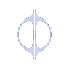
(b)

(c)

(d)

Figure 3.1: Two examples.

We now prove Proposition II.4.

Proof II.6 (Proof of Proposition II.4).

We show both inclusions. First let $\mathcal{\textbf{x}}\in\mathbb{T}_{\mathrm{limit}}$, and we show that $F(\mathcal{\textbf{x}})=0$. In particular, we prove that $0\leq F^{2}(\mathcal{\textbf{x}})<\varepsilon$ for every $\varepsilon>0$.

Let $\varepsilon>0$. Since $F^{2}$ is continuous, there exists $\delta>0$ such that

$${}|\mathcal{\textbf{x}}-\textbf{y}|^{2}<\delta\quad\implies\quad|F^{2}(\mathcal{\textbf{x}})-F^{2}(\textbf{y})|<\textstyle{\frac{\varepsilon}{2}}.$$ (II.2)

After possibly making $\delta$ smaller we can suppose that $\delta<\textstyle{\frac{\varepsilon^{2}}{4}}$.

From the definition of $\mathbb{T}_{\mathrm{limit}}$ (cf. Notation I.4), we have that

$${}\mathbb{T}_{\mathrm{limit}}=\{\mathcal{\textbf{x}}\mid\quad(\forall\delta)(\delta>0\implies(\exists t)(\exists\textbf{y})(\textbf{y}\in\mathbb{T}_{t}\wedge|\mathcal{\textbf{x}}-\textbf{y}|^{2}+t^{2}<\delta))\}.$$ (II.3)

Since $\mathcal{\textbf{x}}\in\mathbb{T}_{\mathrm{limit}}$, there exists $t\in\mathbb{R}_{+}$ and $\textbf{y}\in\mathbb{T}_{t}$ such that $|\mathcal{\textbf{x}}-\textbf{y}|^{2}+t^{2}<\delta$, and in particular both $|\mathcal{\textbf{x}}-\textbf{y}|^{2}<\delta$ and $t^{2}<\delta<\textstyle{\frac{\varepsilon^{2}}{4}}$. The former inequality implies that $|F^{2}(\mathcal{\textbf{x}})-F^{2}(\textbf{y})|<\textstyle{\frac{\varepsilon}{2}}$. The latter inequality implies $t<\textstyle{\frac{\varepsilon}{2}}$, and this together with $\textbf{y}\in\mathbb{T}_{t}$ implies

$$P^{2}(\textbf{y})\leq t(Q^{2}(\textbf{y})-t^{N})$$

$$\implies F^{2}(\textbf{y})Q^{2}(\textbf{y})\leq t(Q^{2}(\textbf{y})-t^{N})$$

$$\implies 0\leq F^{2}(\textbf{y})\leq t-\frac{t^{N+1}}{Q^{2}(\textbf{y})}<t$$

$$\implies 0\leq F^{2}(\textbf{y})<\textstyle{\frac{\varepsilon}{2}}.$$

So, $F^{2}(\textbf{y})<\textstyle{\frac{\varepsilon}{2}}$. Finally, note that $|F^{2}(\mathcal{\textbf{x}})|\leq|F^{2}(\mathcal{\textbf{x}})-F^{2}(\textbf{y})|+|F^{2}(\textbf{y})|<\textstyle{\frac{\varepsilon}{2}}+\textstyle{\frac{\varepsilon}{2}}=\varepsilon$.

We next prove the other inclusion, namely we show ${\rm Zer}(F,\mathbb{R}^{k})\cap\overline{B_{k}(0,R)}\subseteq\mathbb{T}_{\mathrm{limit}}$. Let $\mathcal{\textbf{x}}\in{\rm Zer}(F,\mathbb{R}^{k})\cap\overline{B_{k}(0,R)}$. We fix $\delta>0$ and show that there exists $t\in\mathbb{R}_{+}$ and $\textbf{y}\in\mathbb{T}_{t}$ such that $|\mathcal{\textbf{x}}-\textbf{y}|^{2}+t^{2}<\delta$ (cf. Equation II.3).

There are two cases to consider.

• Since $Q(\mathcal{\textbf{x}})\neq 0$, there exists $t>0$ such that $Q^{2}(\mathcal{\textbf{x}})\geq t^{N}$ and $t^{2}<\delta$. Now, $\mathcal{\textbf{x}}\in\mathbb{T}_{t}$ and

  $$|\mathcal{\textbf{x}}-\mathcal{\textbf{x}}|^{2}+t^{2}\ =\ t^{2}\ <\delta,$$

  so setting $\textbf{y}=\mathcal{\textbf{x}}$ we see that $\textbf{y}\in\mathbb{T}_{t}$ and $|\mathcal{\textbf{x}}-\textbf{y}|+t^{2}<\delta$. Thus, $\mathcal{\textbf{x}}\in\mathbb{T}_{\mathrm{limit}}$ as desired.

• Let $\textbf{v}\in\mathbb{R}^{k}$ be generic, and denote $\widehat{P}(U)=P(\mathcal{\textbf{x}}+U\textbf{v})$, $\widehat{Q}(U)=Q(\mathcal{\textbf{x}}+U\textbf{v})$, and $\widehat{F}(U)=F(\mathcal{\textbf{x}}+U\textbf{v})$. Note that

  $$\widehat{P}=\widehat{F}\widehat{Q},$$

  $$\widehat{P}(0)=\widehat{Q}(0)=\widehat{F}(0)=0.$$ (II.4)

  If $F$ is not the zero polynomial, then neither is $\widehat{P}$, since v is generic. Indeed, assume $F$ is not identically zero, and hence $P$ is not identically zero. In order to prove that $\widehat{P}$ is not identically zero for a generic choice of v, write $P=\sum_{0\leq i\leq d}P_{i}$ where $P_{i}$ is the homogeneous part of $P$ of degree $i$, and $P_{d}$ not identically zero. Then, it is easy to see that $\widehat{P}(U)=P_{d}(\textbf{v})U^{d}+\mathrm{\mbox{lower degree terms}}$. Since $\mathbb{R}$ is an infinite field, a generic choice of v will avoid the set of zeros of $P_{d}$, and thus, $\widehat{P}$ is not identically zero.

  We further require that $\mathcal{\textbf{x}}+t\textbf{v}\in B_{k}(0,R)$ for $t>0$ sufficiently small. For generic v, this is true for either v or $-\textbf{v}$, and so after possibly replacing v by $-\textbf{v}$ (and noticing that since $P_{d}$ is homogeneous we have $P_{d}(\textbf{v})=(-1)^{d}P_{d}(-\textbf{v})$) we may assume $\mathcal{\textbf{x}}+t\textbf{v}\in B_{k}(0,R)$ for $t>0$ sufficiently small. Let $t_{0}>0$ be such that $\mathcal{\textbf{x}}+t\textbf{v}\in B_{k}(0,R)$ for $0<t<t_{0}$.

  Denoting by $\nu=\mathrm{mult}_{0}(\widehat{P})$ and $\mu=\mathrm{mult}_{0}(\widehat{Q})$, we have from ($Q(\mathcal{\textbf{x}})=0$:) that $\nu>\mu$. Let

  $$\widehat{P}(U) =\sum_{i=\nu}^{\deg_{U}\widehat{P}}c_{i}U^{i}=U^{\nu}\cdot\sum_{i=0}^{\deg_{U}\widehat{P}-\nu}c_{\nu+i}U^{i}=c_{\nu}U^{\nu}+\text{ (higher order terms)},$$

  $$\widehat{Q}(U) =\sum_{i=\mu}^{\deg_{U}\widehat{Q}}d_{i}U^{i}=U^{\mu}\cdot\sum_{i=0}^{\deg_{U}\widehat{Q}-\mu}d_{\mu+i}U^{i}=d_{\mu}U^{\mu}+\text{ (higher order terms)}$$

  where $c_{\nu},d_{\mu}\neq 0$.

  Then we have

  $$\widehat{P}^{2}(U) =c_{\nu}^{2}U^{2\nu}+\text{ (higher order terms)},$$

  $$\widehat{Q}^{2}(U) =d_{\mu}^{2}U^{2\mu}+\text{ (higher order terms)},$$

  $$D(U):=U(\widehat{Q}^{2}(U)-U^{N}) =U(d_{\mu}^{2}U^{2\mu}+\text{ (higher order terms)}-U^{N}),$$

  $$D(U)-\widehat{P}^{2}(U) =d_{\mu}^{2}U^{2\mu+1}+\text{ (higher order terms)}-U^{N+1}.$$

  Since $\mu\leq\deg(Q)$ and $N=2\deg(Q)+1$, we have that $2\mu+1<N+1$. Hence, there exists $t_{1}\in\mathbb{R}_{+}$ such that for each $t$, $0<t<t_{1}$, we have $D(t)-\widehat{P}^{2}(t)\geq 0$. Thus, $\mathcal{\textbf{x}}+t\textbf{v}\in\mathbb{T}_{t}$ for each $t$, $0<t<\min\{t_{0},t_{1}\}$. Let $t_{2}=(\frac{\delta}{|\textbf{v}|^{2}+1})^{1/2}$ and note that for all $t$, $0<t<t_{2}$, we have $(|\textbf{v}|^{2}+1)t^{2}<\delta$. Finally, if $t$ satisfies $0<t<\min\{t_{0},t_{1},t_{2}\}$ then $\mathcal{\textbf{x}}+t\textbf{v}\in\mathbb{T}_{t}$, and

  $$|\mathcal{\textbf{x}}-(\mathcal{\textbf{x}}+t\textbf{v})|^{2}+t^{2}\ =\ (|\textbf{v}|^{2}+1)t^{2}<\delta.$$

  Hence, setting $\mathcal{\textbf{y}}=\mathcal{\textbf{x}}+t\textbf{v}$ (cf. Equation II.3) we have shown that $\mathcal{\textbf{x}}\in\mathbb{T}_{\mathrm{limit}}$ as desired.

  The case where $F$ is the zero polynomial is straightforward.

Proof II.7 (Proof of Theorem II.3).

For each $F\in\mathbb{R}[X_{1},\ldots,X_{k}]$, by the conical structure at infinity of semi-algebraic sets (see for instance (BPRbook2, , page 188)), we have that there exists $R_{F}\in\mathbb{R}_{+}$ such that, for every $R>R_{F}$, the semi-algebraic sets ${\rm Zer}(F,\mathbb{R}^{k})\cap\overline{B_{k}(0,R)}$ and ${\rm Zer}(F,\mathbb{R}^{k})$ are semi-algebraically homeomorphic.

Let $\ell\in\mathbb{N}$, $F_{1},\ldots,F_{\ell}\in\mathbb{R}[X_{1},\ldots,X_{k}]$ such that each $F_{i}$ has additive complexity at most $a$ and, for every $F$ having additive complexity at most $a$, the algebraic sets ${\rm Zer}(F,\mathbb{R}^{k}),{\rm Zer}(F_{i},\mathbb{R}^{k})$ are semi-algebraically homeomorphic for some $i$, $1\leq i\leq\ell$ (see, for example (Dries, , Theorem 3.5)). Let $R=\max_{1\leq i\leq\ell}\{R_{F_{i}}\}$.

Let $F\in\{F_{i}\}_{1\leq i\leq\ell}$. By Lemma II.1 there exists polynomials $P,Q\in\mathbb{R}[X_{1},\ldots,X_{k}]$ such that $FQ=P$, and such that $P,Q$ satisfies $P^{2}-T(Q^{2}-T^{N})\in\mathbb{R}[X_{1},\ldots,X_{k},T]$ has division-free additive complexity bounded by $a+2$. Let

$$\mathbb{T}=\{(\mathcal{\textbf{x}},t)\in\mathbb{R}^{k}\times\mathbb{R}_{+}|\;P^{2}(\mathcal{\textbf{x}})\leq t(Q^{2}(\mathcal{\textbf{x}})-t^{N})\wedge|\mathcal{\textbf{x}}|^{2}\leq R^{2}\}.$$

By Proposition II.4 we have that $\mathbb{T}_{\mathrm{limit}}={\rm Zer}(F,\mathbb{R}^{k})\cap\overline{B_{k}(0,R)}.$ Note the one-parameter semi-algebraic family $\mathbb{T}$ (where the last co-ordinate is the parameter) is described by a formula having division-free additive format $(a+k+2,k+1)$.

By Theorem I.1 we obtain a collection of semi-algebraic sets $\mathcal{S}_{k,a+k+2}$ such that $\mathbb{T}_{\mathrm{limit}}$, and hence ${\rm Zer}(F,\mathbb{R}^{k})$, is homotopy equivalent to some $S\in\mathcal{S}_{k,a+k+2}$ and $\#\mathcal{S}_{k,a+k+2}=2^{O(k(k^{2}+a))^{8}}$, which proves the theorem.

II.3 The semi-algebraic case

We first prove a generalization of Proposition II.4.

Notation II.8

Let $\mathbf{X}=(X_{1},\dots,X_{k})$ be a block of variables and $\textbf{k}=(k_{1},\dots,k_{n})\in\mathbb{N}^{n}$ with $\sum_{i=1}^{n}k_{i}=k$. Let $\textbf{r}=(r_{1},\dots,r_{n})\in\mathbb{R}^{n}$ with $r_{i}>0$, $i=1,\dots,n$. Let $B_{\textbf{k}}(0,\textbf{r})$ denote the product

$$B_{\textbf{k}}(0,\textbf{r}):=B_{k_{1}}(0,r_{1})\times\dots\times B_{k_{n}}(0,r_{n}).$$

Notation II.9

For any first order formula $\Phi$ with $k$ free variables, we denote by ${\rm Reali}(\Phi)$ the semi-algebraic subset of $\mathbb{R}^{k}$ defined by $\Phi$.

Proposition II.10.

Let $F_{1},\dots,F_{s},P_{1},\dots,P_{s},Q_{1},\dots,Q_{s}\in\mathbb{R}[\mathbf{X}^{1},\dots,\mathbf{X}^{n}]$, $\mathcal{P}=\{F_{1},\dots,F_{s}\}$ such that $F_{i}Q_{i}=P_{i}$, for all $i=1,\ldots,s$. Suppose $\mathbf{X}^{i}=(X^{i}_{1},\dots,X^{i}_{k_{i}})$ and let $\textbf{k}=(k_{1},\dots,k_{n})$. Suppose $\phi$ is a $\mathcal{P}$-formula containing no negations and no inequalities. Let

$$\bar{P_{i}}:= P_{i}\prod_{j\neq i}Q_{j},$$

$$\bar{Q}:= \prod_{j}Q_{j},$$

and let $\bar{\phi}$ denote the formula obtained from $\phi$ by replacing each $F_{i}=0$ with

$$\bar{P_{i}}^{2}-U(\bar{Q}^{2}-U^{N})\leq 0,$$

where $U$ is the last variable of $\bar{\phi}$, $N=2\deg(\bar{Q})+1$. Then, for every $\emph{{r}}=(r_{1},\dots,r_{n})\in\mathbb{R}_{+}^{n}$, we have (cf. Notation II.9 and Notation I.4)

$${\rm Reali}\left(\bigwedge_{i=1}^{n}(|\mathbf{X}^{i}|^{2}\leq r_{i}^{2})\wedge\bar{\phi}\wedge U>0\right)_{\mathrm{limit}}={\rm Reali}(\phi)\cap\overline{B_{\emph{{k}}}(0,\emph{{r}})}.$$ (II.5)

Proof II.11.

We follow the proof of Proposition II.4. The only case which is not immediate is the case $\mathcal{\textbf{x}}\in{\rm Reali}(\phi)\cap\overline{B_{\textbf{k}}(0,\textbf{r})}$ and $\bar{Q}(\mathcal{\textbf{x}})=0$.

Suppose $\mathcal{\textbf{x}}\in{\rm Reali}(\phi)\cap\overline{B_{\textbf{k}}(0,\textbf{r})}$ and that $\bar{Q}(\mathcal{\textbf{x}})=0$. Since $\phi$ is a formula containing no negations and no inequalities, it consists of conjunctions and disjunctions of equalities. Without loss of generality we can assume that $\phi$ is written as a disjunction of conjunctions, and still without negations. Let

$$\phi=\bigvee_{\alpha}\phi_{\alpha}$$

where $\phi_{\alpha}$ is a conjunction of equations. As above let ${\bar{\phi}_{\alpha}}$ be the formula obtained from $\phi_{\alpha}$ after replacing each $F_{i}=0$ in $\phi_{\alpha}$ with

$$\bar{P_{i}}^{2}\leq U(\bar{Q}^{2}-U^{N}),$$

$N=2\deg(\bar{Q})+1$.

We have

$${\rm Reali}\left(\bigwedge_{i=1}^{p}(|\mathbf{X}^{i}|^{2}\leq r_{i}^{2})\wedge\bar{\phi}\wedge U>0\right)_{\mathrm{limit}} ={\rm Reali}\left(\bigwedge_{i=1}^{p}(|\mathbf{X}^{i}|^{2}\leq r_{i}^{2})\wedge\left(\bigvee_{\alpha}{\bar{\phi}_{\alpha}}\right)\wedge U>0\right)_{\mathrm{limit}}$$

$$={\rm Reali}\left(\bigvee_{\alpha}\bigwedge_{i=1}^{p}(|\mathbf{X}^{i}|^{2}\leq r_{i}^{2})\wedge{\bar{\phi}_{\alpha}}\wedge U>0\right)_{\mathrm{limit}}$$

$$=\bigcup_{\alpha}{\rm Reali}\left(\bigwedge_{i=1}^{p}(|\mathbf{X}^{i}|^{2}\leq r_{i}^{2})\wedge{\bar{\phi}_{\alpha}}\wedge U>0\right)_{\mathrm{limit}}.$$

In order to show that $\mathcal{\textbf{x}}\in{\rm Reali}\left(\bigwedge_{i=1}^{p}(|\mathbf{X}^{i}|^{2}\leq r_{i}^{2})\wedge\bar{\phi}\wedge U>0\right)_{\mathrm{limit}}$ it now suffices to show that if $\mathcal{\textbf{x}}\in{\rm Reali}(\phi_{\alpha})\cap\overline{B_{\textbf{k}}(0,\textbf{r})}$ and $\bar{Q}(\mathcal{\textbf{x}})=0$, then x belongs to ${\rm Reali}\left(\bigwedge_{i=1}^{p}(|\mathbf{X}^{i}|^{2}\leq r_{i}^{2})\wedge{\bar{\phi}_{\alpha}}\wedge U>0\right)_{\mathrm{limit}}$.

Let $\mathcal{\textbf{x}}\in{\rm Reali}(\phi_{\alpha})\cap\overline{B_{\textbf{k}}(0,\textbf{r})}$ and suppose $\bar{Q}(\mathcal{\textbf{x}})=0$. Let $\mathcal{Q}\subseteq\mathcal{P}$ consist of the polynomials of $\mathcal{P}$ appearing in $\phi_{\alpha}$. Let $\textbf{v}\in\mathbb{R}^{k}$ be generic, and denote $\widehat{P_{i}}(U)=\bar{P_{i}}(\mathcal{\textbf{x}}+U\textbf{v})$, $\widehat{Q}(U)=\bar{Q}(\mathcal{\textbf{x}}+U\textbf{v})$, and $\widehat{F_{i}}(U)=\bar{F}(\mathcal{\textbf{x}}+U\textbf{v})$. Note that

$$\widehat{P_{i}}=\widehat{F_{i}}\widehat{Q},$$

$$\widehat{P_{i}}(0)=\widehat{Q}(0)=\widehat{F_{i}}(0)=0.$$ (II.6)

As in the proof of Proposition II.4, if $F_{i}\in\mathcal{Q}$ is not the zero polynomial then $\widehat{P_{i}}$ is not identically zero. Since $\phi_{\alpha}$ consists of a conjunction of equalities and

$$\bigwedge_{F\in\mathcal{Q}\atop F\not\equiv 0}F=0\iff\bigwedge_{F\in\mathcal{Q}}F=0,$$

we may assume that $\mathcal{Q}$ does not contain the zero polynomial. Under this assumption, we have that for every $F_{i}\in\mathcal{Q}$ the univariate polynomial $\widehat{P_{i}}$ is not identically zero. As in the proof of Proposition II.4, there exists $t_{0}\in\mathbb{R}_{+}$ such that for all $t$, $0<t<t_{0}$, we have $\mathcal{\textbf{x}}+t\textbf{v}\in B_{\textbf{k}}(0,\textbf{r})$. Denoting by $\nu_{i}=\mathrm{mult}_{0}(\widehat{P_{i}})$ and $\mu=\mathrm{mult}_{0}(\widehat{Q})$, we have from (II.11) that $\nu_{i}>\mu$ for all $i=1,\dots,s$.

Let

$$\widehat{P_{i}}(U) =\sum_{j=\nu_{i}}^{\deg_{U}\widehat{P_{i}}}c_{j}U^{j}=U^{\nu_{i}}\cdot\sum_{j=0}^{\deg_{U}\widehat{P_{i}}-\nu_{i}}c_{\nu_{i}+j}U^{j}=c_{\nu_{i}}U^{\nu_{i}}+\text{ (higher order terms)},$$

$$\widehat{Q}(U) =\sum_{j=\mu}^{\deg_{U}\widehat{Q}}d_{j}^{j}=U^{\mu}\cdot\sum_{j=0}^{\deg_{U}\widehat{Q}-\mu}d_{\mu+j}U^{j}=d_{\mu}U^{\mu}+\text{ (higher order terms)}$$

where $d_{\mu}\neq 0$ and $c_{\nu_{i}}\neq 0$.

Then we have

$$\widehat{P_{i}}^{2}(U) =c_{\nu_{i}}^{2}U^{2\nu_{i}}+\text{ (higher order terms)},$$

$$\widehat{Q}^{2}(U) =d_{\mu}^{2}U^{2\mu}+\text{ (higher order terms)},$$

$$D(t):=U(\widehat{Q}^{2}(U)-U^{N}) =U(d_{\mu}^{2}U^{2\mu}+\text{ (higher order terms)}-U^{N}),$$

$$D(U)-\widehat{P_{i}}^{2}(U) =d_{\mu}^{2}U^{2\mu+1}+\text{ (higher order terms)}-U^{N+1}.$$

Since $\mu\leq\deg(\bar{Q})$ and $N=2\deg(\bar{Q})+1$, we have that $2\mu+1<N+1$. Hence, there exists $t_{1,i}\in\mathbb{R}_{+}$ such that for all $t$, $0<t<t_{1,i}$, we have that $D(t)-\widehat{P_{i}}^{2}(t)\geq 0$, and thus $\mathcal{\textbf{x}}+t\textbf{v}$ satisfies

$$\bar{P}_{i}^{2}(\mathcal{\textbf{x}}+t\textbf{v})\leq t(\bar{Q}^{2}(\mathcal{\textbf{x}}+t\textbf{v})-t^{N}).$$

Let $t_{1}=\min\{t_{1,1},\dots,t_{1,s}\}$. Let $t_{2}=(\frac{\delta}{|\textbf{v}|^{2}+1})^{1/2}$ and note that for all $t\in\mathbb{R}$, $0<t<t_{2}$, we have $(|\textbf{v}|^{2}+1)t^{2}<\delta$. Finally, if $t$ satisfies $0<t<\min\{t_{0},t_{1},t_{2}\}$ then

$$(\mathcal{\textbf{x}}+t\textbf{v},t)\in{\rm Reali}\left(\bigwedge_{i=1}^{p}(|\mathbf{X}^{i}|^{2}\leq r_{i}^{2})\wedge{\bar{\phi}_{\alpha}}\wedge U>0\right)$$

and

$$|\mathcal{\textbf{x}}-(\mathcal{\textbf{x}}+t\textbf{v})|^{2}+t^{2}\ =\ (|\textbf{v}|^{2})t^{2}<\delta,$$

and so we have shown that

$$\mathcal{\textbf{x}}\in{\rm Reali}\left(\bigwedge_{i=1}^{p}(|\mathbf{X}^{i}|^{2}\leq r_{i}^{2})\wedge{\bar{\phi}_{\alpha}}\wedge U>0\right)_{\mathrm{limit}}.$$

Using the same notation as in Proposition II.10 above:

Corollary II.12.

Let $\phi$ be a $\mathcal{P}$-formula, containing no negations and no inequalities, with $\mathcal{P}\subset\textnormal{{R}}[X_{1},\ldots,X_{k}]$ with $\mathcal{P}\in\mathcal{A}_{k,a}$. Then, there exists a family of polynomials $\mathcal{P}^{\prime}\subset\textnormal{{R}}[X_{1},\ldots,X_{k},U]$, and a $\mathcal{P}^{\prime}$-formula $\bar{\phi}$ satisfying (II.5), and such that $\mathcal{P}^{\prime}\in\mathcal{A}^{\mathrm{div-free}}_{k+1,(k+a)(a+2)}$.

Proof II.13.

The proof is immediate from Lemma II.1, Remark .13, and the definition of $\bar{\phi}$.

Definition II.14.

Let $\Phi$ be a $\mathcal{P}$-formula, $\mathcal{P}\subseteq\mathbb{R}[\mathbf{X}_{1},\dots,\mathbf{X}_{k}]$, and say that $\Phi$ is a $\mathcal{P}$-closed formula if the formula $\Phi$ contains no negations and all the inequalities in atoms of $\Phi$ are weak inequalities.

Let $\mathcal{P}=\{F_{1},\ldots,F_{s}\}\subset\mathbb{R}[X_{1},\ldots,X_{k}]$, and $\Phi$ a $\mathcal{P}$-closed formula.

For $R\in\mathbb{R}_{+}$, let $\Phi_{R}$ denote the formula $\Phi\wedge(|\mathbf{X}|^{2}-R^{2}\leq 0)$.

Let $\Phi^{\dagger}$ be the formula obtained from $\Phi$ by replacing each occurrence of the atom $F_{i}\ast 0$, $\ast\in\{=,\leq,\geq\}$, $i=1,\dots,s$, with

$$F_{i}-V_{i}^{2}=0 \mbox{ if }\ast\in\{\leq\},$$

$$-F_{i}-V_{i}^{2}=0 \mbox{ if }\ast\in\{\geq\},$$

$$F_{i}=0 \mbox{ if }\ast\in\{=\},$$

and for $R,R^{\prime}\in\mathbb{R}_{+}$, let $\Phi^{\dagger}_{R,R^{\prime}}$ denote the formula

$$\Phi^{\dagger}\wedge(U_{1}^{2}+|\mathbf{X}|^{2}-R^{2}=0)\wedge(U_{2}^{2}+|\mathbf{V}|^{2}-R^{\prime 2}=0).$$

We have

Proposition II.15.

$${\rm Reali}(\Phi)=\pi_{[1,k]}({\rm Reali}(\Phi^{\dagger})),$$

and for all $0<R\ll R^{\prime}$,

$${\rm Reali}(\Phi_{R})=\pi_{[1,k]}({\rm Reali}(\Phi^{\dagger}_{R,R^{\prime}})),$$

Proof II.16.

Obvious.

Note that, for $0<R\ll R^{\prime}$, $\pi_{[1,k]}|_{{\rm Reali}(\Phi^{\dagger}_{R,R^{\prime}})}$ is a continuous, semi-algebraic surjection onto ${\rm Reali}(\Phi_{R})$. Let $\pi_{R,R^{\prime}}$ denote the map $\pi_{[1,k]}|_{{\rm Reali}(\Phi^{\dagger}_{R,R^{\prime}})}$.

Proposition II.17.

We have that $\mathcal{J}^{p}_{\pi_{R,R^{\prime}}}({\rm Reali}(\Phi^{\dagger}_{R,R^{\prime}}))$ is $p$-equivalent to $\pi_{[1,k]}({\rm Reali}(\Phi^{\dagger}_{R,R^{\prime}}))$. Moreover, for any two formulas $\Phi,\Psi$, the realizations ${\rm Reali}(\Phi)$ and ${\rm Reali}(\Psi)$ are homotopy equivalent if, for all $1\ll R\ll R^{\prime}$,

$${\rm Reali}(\mathcal{J}^{p}_{\pi_{R,R^{\prime}}}(\Phi^{\dagger}_{R,R^{\prime}}))\simeq{\rm Reali}(\mathcal{J}^{p}_{\pi_{R,R^{\prime}}}(\Psi^{\dagger}_{R,R^{\prime}}))$$

are homotopy equivalent for some $p>k$.

Proof II.18.

Immediate from Proposition I.15 and Propositions IV.1 and II.15.

Suppose that $\Phi$ has additive format bounded by $(a,k)$, and suppose that the number of polynomials appearing $\Phi$ is $s$, and without loss of generality we can assume that $s\leq k+a$ (see Remark .13). Then the sum of the additive complexities of the polynomials appearing in $\Phi^{\dagger}_{R,R^{\prime}}$ is bounded by $3a+3s+2\leq 3a+3(a+k)+2\leq 6(k+a)$, and the formula $\Phi^{\dagger}_{R,R^{\prime}}$ has additive format bounded by $(6(k+a),2k+a+2)$. Consequently, the additive format of the formula

$$\Theta_{1}\wedge\Theta_{2}^{\Phi^{\dagger}_{R,R^{\prime}}}\wedge\Theta_{3}^{\pi_{R,R^{\prime}}}$$

is bounded by $(M,N)$,

$$M =(p+1)(6k+6a+1)+\textstyle{\binom{p+1}{2}}(4k+2a+3)$$

$$N =(p+1)(2k+a+3)+\textstyle{\binom{p+1}{2}}.$$

In the above, the estimates of Proposition I.27 suffice, with $(a,k)$ replaced by $(6(k+a),2k+a+2)$. Now, applying Corollary II.12 we have that there exists a $\mathcal{P}^{\prime}$-formula

$$\overline{\left(\Theta_{1}\wedge\Theta_{2}^{\Phi^{\dagger}_{R,R^{\prime}}}\wedge\Theta_{3}^{\pi_{R,R^{\prime}}}\right)}$$

which satisfies Equation II.5 and such that the division-free additive format of this formula is bounded by $((N+M)(M+2),N+1)$. Finally, let $\mathcal{J}^{p}_{\pi_{R,R^{\prime}}}(\Phi^{\dagger}_{R,R^{\prime}})^{\star}$ denote the formula, with last variable $U$,

$${}\Omega^{R}\wedge\overline{\left(\Theta_{1}\wedge\Theta_{2}^{\Phi^{\dagger}_{R,R^{\prime}}}\wedge\Theta_{3}^{\pi_{R,R^{\prime}}}\right)}\wedge U>0,$$ (II.7)

and we have that the division-free additive format of $\mathcal{J}^{p}_{\pi_{R,R^{\prime}}}(\Phi^{\dagger}_{R,R^{\prime}})^{\star}$ is bounded by $(M^{\prime},N+1)$,

$$M^{\prime}=(p+1)(2k+a+3)+(N+M)(M+2).$$

Note that $M^{\prime}\leq 5M^{2}$.

We have shown the following,

Proposition II.19.

Suppose that the sum of the additive complexities of $F_{i},1\leq i\leq s$, is bounded by $a$. Then, the semi-algebraic set ${\rm Reali}(\mathcal{J}^{p}_{\pi_{R,R^{\prime}}}(\Phi^{\dagger}_{R,R^{\prime}})^{\star})$ can be defined by a $\mathcal{P}^{\prime}$-formula with $\mathcal{P}^{\prime}\in\mathcal{A}^{\mathrm{div-free}}_{5M^{2},N+1}$,

$$M =(p+1)(6k+6a+1)+2\textstyle{\binom{p+1}{2}}(4k+2a+3)$$

$$N =(p+1)(2k+a+3)+\textstyle{\binom{p+1}{2}}.$$

Finally, we obtain

Proposition II.20.

The number of distinct homotopy types of semi-algebraic subsets of $\mathbb{R}^{k}$ defined by $\mathcal{P}$-closed formulas with $\mathcal{P}\in\mathcal{A}_{a,k}$ is bounded by $2^{(k(k+a))^{O(1)}}$.

Proof II.21.

Let $\mathcal{P}\in\mathcal{A}_{a,k}$. By the conical structure at infinity of semi-algebraic sets (see, for instance (BPRbook2, , page 188)) there exists $R_{\mathcal{P}}>0$ such that, for all $R>R_{\mathcal{P}}$ and every $\mathcal{P}$-closed formula $\Phi$, the semi-algebraic sets ${\rm Reali}(\Phi_{R}),{\rm Reali}(\Phi)$ are semi-algebraically homeomorphic.

For each $a,k\in\mathbb{N}$, there are only finitely many semi-algebraic homeomorphism types of semi-algebraic sets described by a $\mathcal{P}$-formula having additive complexity at most $(a,k)$ (Dries, , Theorem 3.5). Let $\ell\in\mathbb{N}$, $\mathcal{P}_{i}\in\mathcal{A}_{a,k}$, and $\Phi_{i}$ a $\mathcal{P}_{i}$-formula, $1\leq i\leq\ell$, such that every semi-algebraic set described by a formula of additive complexity at most $(a,k)$ is semi-algebraically homeomorphic to ${\rm Reali}(\Phi_{i})$ for some $i$, $1\leq i\leq\ell$. Let $R=\max_{1\leq i\leq\ell}\{R_{\mathcal{P}_{i}}\}$ and $R^{\prime}\gg R$.

Let $\Phi\in\{\Phi_{i}\}_{1\leq i\leq\ell}$. By Proposition II.17 it suffices to bound the number of distinct homotopy types of the semi-algebraic set ${\rm Reali}(\mathcal{J}^{k+1}_{\pi_{R,R^{\prime}}}(\Phi^{\dagger}_{R,R^{\prime}}))$. By Proposition II.10, we have that

$${\rm Reali}\left(\mathcal{J}^{k+1}_{\pi_{R,R^{\prime}}}(\Phi^{\dagger}_{R,R^{\prime}})^{\star}\right)_{\mathrm{limit}}={\rm Reali}(\mathcal{J}^{k+1}_{\pi_{R,R^{\prime}}}(\Phi^{\dagger}_{R,R^{\prime}})).$$

By Proposition II.19, the division-free additive format of the formula $\mathcal{J}^{k+1}_{\pi_{R,R^{\prime}}}(\Phi^{\dagger}_{R,R^{\prime}})^{\star}$ is bounded by $(2M,N)$, where $p=k+1$. The proposition now follows immediately from Theorem I.1.

Proof II.22 (Proof of Theorem .11).

Using the construction of Gabrielov and Vorobjov GV07 one can reduce the case of arbitrary semi-algebraic sets to that of a closed and bounded one, defined by a $\mathcal{P}$-closed formula, without changing asymptotically the complexity estimates (see for example BV06 ). The theorem then follows directly from Proposition II.20 above.

II.4 Proof of Theorem I.5

Proof II.23 (Proof of Theorem I.5).

The proof is identical to that of the proof of Theorem I.1, except that we use Theorem .11 instead of Theorem .6.

Chapter 4 Semi-cylindrical decomposition

Decomposition theorems are ubiquitous in real algebraic geometry as well as in computational geometry, used to study the topology of semi-algebraic sets or used, for example, in point location algorithms. In the latter case, given a subset $X$ of $\textnormal{{R}}^{k}$ in some well-behaved class of sets (e.g., $X$ is a polygon, definable, semi-algebraic, etc.), the goal is to partition $\textnormal{{R}}^{k}$ into sets, typically called cells of the decomposition, such that the union of cells in some sub-collection of this partition is $X$.

For a concrete example, we turn to the well-known cylindrical decomposition for semi-algebraic sets. This decomposition theorem provides a partition of $\textnormal{{R}}^{k}$ into finitely many cells so that the union of some sub-collection of the cells is $X$. The cells in this case are semi-algebraic and have bounded description complexity in that they are all semi-algebraic and can be described using a finite list of polynomials, whose number and degree are bounded by a function of the number and maximum degree of the polynomials appearing in a description of $X$. Partitions of this type are sometimes called Tarski decompositions in the literature. A typical quantitative question one can ask is, given $X_{1},\ldots,X_{n}$ subsets of $\textnormal{{R}}^{k}$, can one prove existence of decomposition of $\textnormal{{R}}^{k}$ into sets of bounded description complexity such that the number of the sets in the decomposition is as few as possible, bounded by a function of $n,k$ and the description complexity of the sets $X_{1},\ldots,X_{n}$.

Another example of a Tarski decomposition, a finite partition of $\textnormal{{R}}^{k}$ into sets of bounded description complexity, coming from computational geometry is that of $\varepsilon$-cuttings matousek1995approximations . A cutting is a collection of (possibly unbounded) simplices with disjoint interiors which cover $\textnormal{{R}}^{k}$. Given a set $\mathcal{H}$ of $n$ hyperplanes in $\textnormal{{R}}^{k}$, an $\varepsilon$-cutting is a cutting $\Delta$ such that for every simplex $s\in\Delta$ the numbef of hyperplanes in $\mathcal{H}$ which intersect the interior of $s$ is at most $\varepsilon n$. It was proved by Chazelle and Friedman in chazelle1990deterministic that for any $n$ hyperplanes and any $r\leq n$ an $(1/r)$-cutting exists of size $O(r^{k})$, and that there exists an algorithm for computing this cutting. The technique of $\varepsilon$-cuttings have been used by many authors to make progress on several problems in computational geometry as the divide step in several divide-and-conquer arguments where a problem (e.g., point location, incidence problems) is broken up into several easier to handle problems.

It is often the case that one is primarily concerned with the asymptotic behaviour of the number of sets in the partition as the number of sets to be partitioned increases, while treating the description complexity of $X$ the sets and the dimension of the ambient space $k$ as constants. In these settings, it is the combinatorial part of the bounds that are relevant, as opposed to the algebraic part of the bounds. Loosely speaking, the combinatorial part of a bound is the part that depends on $n$ the number of sets and the dimension $k$ of the ambient space, while the algebraic part is the part that depends on the description complexity of the sets involved.

When one is primarily concerned with the combinatorial part of the complexity of a decomposition, then the setting of o-minimal geometry and definable sets is an appropriate framework for analyzing the problem. In this setting, the role of bounded description complexity is replaced by having all the sets involved arise as fibers of a single definable set in a larger space, which parametrizes the family from which the sets involved are taken. In this way the combinatorial part of the bound is brought into focus while the algebraic part is subsumed as part of the dimension of the ambient space. When one reads the statement of the following theorems it may help to keep this in mind. In order to state the theorems we define the structure of a cylindrical decomposition.

A cylindrical definable decomposition, or cdd, of $\textnormal{{R}}^{k}$ is a partition of $\textnormal{{R}}^{k}$ into finitely many definable sets of a particular type, namely that these sets are defined inductively as follows.

• A cdd of R consists of a finite set of points $a_{1}<\ldots<a_{m}$ of R and the set of maximal open intervals $(-\infty,a_{1}),(a_{1},a_{2}),\ldots,(a_{m-1},a_{m}),(a_{m},\infty)$ in the complement of those points in R.

• A cdd of $\textnormal{{R}}^{k}$ with $k>1$ consists of a cdd, $\{C_{\alpha}\}_{\alpha\in I}$, of $\textnormal{{R}}^{k-1}$ and for each $\alpha\in I$ a cdd $\{A_{\beta}\}_{\beta\in J}$ of R and definable homeomorphisms $\phi_{\alpha,\beta}:C_{\alpha}\times A_{\beta}\to Y_{\alpha,\beta}$ satisfying $\pi^{k}_{\leq k-1}\circ\phi_{\alpha,\beta}=\pi^{k}_{\leq k-1}$ and which satisfy $\{Y_{\alpha,\beta}\}_{\alpha,\beta}$ is a partition of $\textnormal{{R}}^{k}$. The cdd of $\textnormal{{R}}^{k}$ is then given by $\{Y_{\alpha,\beta}\}_{\alpha\in I,\beta\in J}$.

We make the following inductive definition, that of a cylindrical set.

• A cylindrical set of R is a point $a\in\textnormal{{R}}$ or the open interval $(a,b)$ between two points $a,b\in\textnormal{{R}}$.

• Given a cylindrical set $X$ of $\textnormal{{R}}^{k-1}$ and definable continuous functions $\xi,\xi_{1},\xi_{2}:Y\to\textnormal{{R}}$ satisfying $\xi_{1}(x)<\xi_{2}(x)$ for all $x\in X$, a cylindrical set $Y$ of $\textnormal{{R}}^{k}$ is either a graph of the form $Y=\{(x,a)\in\textnormal{{R}}^{k}|\;\xi(x)=a\}$ or a band of the form $\{(x,a)\in\textnormal{{R}}^{k}|\;\xi_{1}(x)<a<\xi_{2}(x)\}$.

A partition of $\textnormal{{R}}^{k}$ into definable sets is called a semi-cylindrical decomposition if each cell of the decomposition is a cylindrical set. As we will see, a semi-cylindrical decomposition need not have a cylindrical structure, in that given a cell $Y$ of a semi-cylindrical decomposition of $\textnormal{{R}}^{k}$, it need not be the case that the cylinder $\pi^{k}_{\leq k-1}(Y)\times R$ is a union of cells of the decomposition.

A subset $A$ of $\textnormal{{R}}^{k}$ is said to be compatible with a set $X$ if $A\subseteq X$ or $A\cap X=\emptyset$, and if $\mathcal{A}$ is a partition of $\textnormal{{R}}^{k}$ and $X_{1},\ldots,X_{n}$ are subsets of $\textnormal{{R}}^{k}$ such that $A$ is compatible with $X_{1},\ldots,X_{n}$ for every $A\in\mathcal{A}$, then $\mathcal{A}$ is said to be adapted to $X_{1},\ldots,X_{n}$.

Let $R$ be a real closed field.

The following theorem is proved in Basu9 .

Theorem .1 (Quantitative cylindrical definable decomposition Basu9 ).

Let $T\subseteq\textnormal{{R}}^{k+\ell}$ be a definable set, then there exists constants $C_{1},C_{2}$ and a finite family of definable sets $\mathcal{A}$, $|\mathcal{A}|\leq C_{1}$, and

$$A\subseteq\textnormal{{R}}^{k}\times\textnormal{{R}}^{2(2^{k}-1)\ell},\;A\in\mathcal{A},$$

which satisfy the following property. For any $n$ points $y_{1},\ldots,y_{n}\in\textnormal{{R}}^{\ell}$, some sub-collection of the sets

$$\pi^{k+2(2^{k}-1)\ell}_{\leq k}\left({(\pi^{k+2(2^{k}-1)\ell}_{>k})}^{-1}(y_{i_{1}},\ldots,y_{i_{2(2^{k}-1)}})\quad\cap\quad A\right),$$

$A\in\mathcal{A}$ and $1\leq i_{1},\ldots,i_{2(2^{k}-1)}\leq n$, form a cylindrical definable decomposition adapted to $T_{y_{1}},\ldots,T_{y_{n}}$. Also, the number of sets in the decomposition is bounded by $C_{2}n^{2^{k}-1}$.

We prove a theorem which is weaker in that it does not ensure a cylindrical structure to the decomposition, yet the number of sets required is asymptotically better and still the cells of the decomposition are of constant description complexity.

Theorem .2 (Quantitative semi-cylindrical definable decomposition).

Let $T\subseteq\textnormal{{R}}^{k+\ell}$ be a definable set, then there exists constants $C_{1},C_{2}$ and a finite family of definable sets $\mathcal{A}$, $|\mathcal{A}|\leq C_{1}$, and

$$A\subseteq\textnormal{{R}}^{k}\times\textnormal{{R}}^{2(2^{k}-1)\ell},\;A\in\mathcal{A},$$

which satisfy the following property. For any $n$ points $y_{1},\ldots,y_{n}\in\textnormal{{R}}^{\ell}$, some sub-collection of the sets

$$\pi^{k+2(2^{k}-1)\ell}_{\leq k}\left({(\pi^{k+2(2^{k}-1)\ell}_{>k})}^{-1}(y_{i_{1}},\ldots,y_{i_{2(2^{k}-1)}})\quad\cap\quad A\right),$$

$A\in\mathcal{A}$ and $1\leq i_{1},\ldots,i_{2(2^{k}-1)}\leq n$, form a semi-cylindrical decomposition of $\textnormal{{R}}^{k}$ adapted to $T_{y_{1}},\ldots,T_{y_{n}}$. Also, the number of sets in the decomposition is bounded by $C_{2}n^{2k-1}$.

I Some preliminaries

We first make some preliminary definitions.

I.1 o-minimal structures

A structure $\mathcal{S}(\textnormal{{R}})$ on R is a collection families of subsets of $\textnormal{{R}}^{\ell}$, $\{\mathcal{S}_{\ell}\}_{\ell\geq 1}$, satisfying:

1. all algebraic subsets of $\textnormal{{R}}^{\ell}$ are in $\mathcal{S}_{\ell}$,

2. each family $\mathcal{S}_{\ell}$ is a boolean algebra, i.e., closed under finite unions, intersections and taking complements,

3. for $A\in\mathcal{S}_{m}$ and $B\in\mathcal{S}_{n}$, we have $A\times B\in\mathcal{S}_{m+n}$.

4. if $\pi^{n+1}_{\leq n}:R^{n+1}\to\textnormal{{R}}^{n}$ is the projection map which forgets the last coordinate and $A\in S_{n+1}$, then $\pi^{n+1}_{\leq n}(A)\in S_{n}$.

If additionally

1. the elements of $\mathcal{S}_{1}$ are precisely finite unions of points and open intervals,

then the structure is said to be o-minimal. For any structure $\mathcal{S}(\textnormal{{R}})$, a set $A\subseteq\textnormal{{R}}^{\ell}$ is said to be definable in the structure $\mathcal{S}(\textnormal{{R}})$ if $A\in\mathcal{S}_{\ell}$.

Remark I.1.

It is well known that the collection of semi-algebraic subsets over R, sets defined by a boolean combination of real polynomial equalities and inequalities, is an o-minimal structure. The non-trivial but well known fact that the collection of semi-algebraic subsets is closed under taking projections follows from the Tarski-Seidenberg quantifier elimination Theorem BPRbook2 .

I.2 Endpoints and adapted partitions

Two definitions that will be important in our exposition are that of the endpoints of a definable subset of R and the common refinement of a definable subset of R. Endpoints of a definable subset $A$ of R are those elements in R which are on the boundary of the definable set. Their number is finite (see Lemma I.5), and the set of endpoints of $A$ and the set of maximal open intervals in their complement comprise the coarsest partition of R which is a cdd and which is adapted to $A$, which we refer to as the common refinement of $A$. More precisely,

Definition I.2.

The set of endpoints of $A$ is the set $\textrm{clos}{A}\smallsetminus\textrm{int}{A}$, where the closure $\textrm{clos}{A}$ of $A$ and interior $\textrm{int}{A}$ of $A$ are taken in the order topology of R (or the Euclidean topology if the language contains $+,\times$).

Lemma I.3.

Let $A_{1},\ldots,A_{n}\subseteq\textnormal{{R}}$ be definable. Then the set of endpoints of $\cup_{1\leq i\leq n}A_{i}$ is contained in the union of the sets of endpoints of $A_{i}$, $1\leq i\leq n$. In symbols,

$${}\displaystyle\textrm{clos}\left(\cup_{1\leq i\leq n}A_{i}\right)\smallsetminus\textrm{int}\left(\cup_{1\leq i\leq n}A_{i}\right)\subseteq\bigcup_{1\leq i\leq n}\textrm{clos}(A_{i})\smallsetminus\textrm{int}(A_{i}).$$ (I.1)

Proof I.4.

Equation I.1 can be shown to hold for arbitrary sets $A_{i}$, $1\leq i\leq n$, in any topological space $X$ using elementary point set topology (e.g., Munkres). The lemma then follows from the definitions.

Lemma I.5.

Given a definable subset $A\subseteq\textnormal{{R}}$, the set of endpoints of $A$ is a finite definable subset of R.

Proof I.6.

The set of endpoints of a point $\{a\}$ is the set $\{a\}$, and the set of endpoints of an interval $(a,b)$ is the set $\{a,b\}$. By Lemma I.3 and the fact that $A$ is a finite union of points and intervals, the set of endpoints of $A$ is finite, hence definable by definition.

The common refinement of a definable subset $A$ of R (see Definition I.9 below) is the coarsest cdd of R adapted to $A$. We also provide definitions of other adapted partitions, beginning with the basic boolean algebra generated by an arrangement, which is the coarsest partition of a set $X$ adapted to subsets $A_{1},\ldots,A_{n}$, and whose definition already appeared in Basu9 .

Notation I.7

Basu9 Let $\mathcal{A}=\{A_{1},\dots,A_{n}\}$ be a collection of subsets of a set $X$. Let $I\subseteq\{1,\dots,n\}$, allowing $I=\emptyset$ with the convention that if $I=\emptyset$ then the intersection over an empty index set is $X$, $\cap_{i\in\emptyset}A_{i}=X$. Let $\mathcal{A}(I)$ denote the set

$$\left(\bigcap_{i\in I}A_{i}\right)\setminus\left(\bigcup_{i\notin I}A_{i}\right),$$

and we call each such set a basic $\mathcal{A}$-set.

Definition I.8 (Boolean algebra generated by an arrangement Basu9 ).

The   basic boolean algebra of $X$ generated by $\mathcal{A}=\{A_{1},\dots,A_{n}\}$, denoted $\mathcal{B}^{\ast}(A_{1},\dots,A_{n})$ or just $\mathcal{B}^{\ast}(\mathcal{A})$, is the collection of basic $\mathcal{A}$-sets

$$\mathcal{B}^{\ast}(A_{1},\dots,A_{n})=\{\mathcal{A}(I)|\ I\subset\{1,\dots,n\}\}.$$

We use the notation $\mathcal{B}(A_{1},\dots,A_{n})$ to denote the set of connected components of sets in $\mathcal{B}^{\ast}(A_{1},\dots,A_{n})$ and call the set of connected components the boolean algebra of $X$ generated by $A_{1},\dots,A_{n}$.

We will use the next definition in the proof of the main theorem in an essential way. We need to have a slightly finer partition than the boolean algebra generated by an arrangement in order to make cylindrical cells; this is related to the separate roles of graphs and bands in the more familiar cylindrical decomposition theorem for semi-algebraic sets.

Definition I.9 (Common refinement).

Let $A_{1},\ldots,A_{n}\subseteq\textnormal{{R}}$ be definable sets and define the common refinement of the sets $A,B$ as the union of the sets of endpoints of $A_{i}$, $1\leq i\leq n$, and the set of maximal open intervals in the complement in R of these endpoints.

Definition I.10 (Adapted partition).

For a partition of a set $X=\sqcup_{\alpha\in I}C_{\alpha}$ into pairwise disjoint sets $C_{\alpha}$, we say that the partition $\{C_{\alpha}\}$ is adapted to the sets $S_{1},S_{2},\dots,S_{n}$ with $S_{i}\subseteq X$ if for each $i=1,\dots,n$ we have

$$\forall\alpha\in I\quad C_{\alpha}\cap S_{i}=\emptyset\quad\text{or}\quad C_{\alpha}\subseteq S_{i}.$$

Given a collection of subsets $\mathcal{A}$ of a set $X$, the collection of sets $\mathcal{B}^{\ast}(A_{1},\ldots,A_{n})$ is the coarsest partition of $X$ which is adapted to the sets in $\mathcal{A}$. Additionally, the sets in the common refinement of definable sets $A,B\subseteq\textnormal{{R}}$ comprise the coarsest partition of R adapted to $A$ and $B$ into sets which are either points or open intervals. For example, $\mathcal{B}([0,1))=\{(-\infty,0),[0,1),[1,\infty)\}$ and the common refinement of $[0,1)$ is the partition $\{(-\infty,0),\{0\},(0,1),\{1\},(1,\infty)\}$.

I.3 Hardt’s Theorem

We next state the o-minimal version of Hardt’s Theorem, which provides the main technical tool for the proof of the main result of this section. The version stated here is taken from Basu9 .

Definition I.11 (Definably trivial maps).

Let $X\subseteq\textnormal{{R}}^{n+m}$ and $C\subseteq\textnormal{{R}}^{m}$ be definable, and let $\pi:X\to\textnormal{{R}}^{k}$ denote the projection map which forgets the last $m$ coordinates. We say that $X$ is definably trivial over $C$ if there exists a definable set $A\subseteq\textnormal{{R}}^{n}$ and map $h$, called the trivialization of $X$ over $C$, such that

1. $h$ is a definable homeomorphism $h:A\times C\to X\cap\pi^{-1}(C)$, and

2. $\pi\circ h=\pi$.

If $Y$ is a definable subset of $X$, we say that the trivialization of $X$ over $C$ is compatible with $Y$ if there exists a definable subset $B$ of $A$ satisfying $h(B\times C)=Y\cap\pi^{-1}(C)$.

Theorem I.12 (Hardt’s theorem for definable families Basu9 ).

Let $X\subseteq\textnormal{{R}}^{k+\ell}$ be a definable set and let $Y_{1},\dots,Y_{m}$ be definable subsets of $X$. Then, there exists a finite partition of $R^{\ell}$ into definable sets $C_{1},\dots,C_{N}$ such that $X$ is definably trivial over each $C_{i}$, and moreover the trivialization over each $C_{i}$ is compatible with $Y_{1},\dots,Y_{m}$.

The following two corollaries follow immediately from Hardt’s theorem and the proofs are omitted.

Corollary I.13.

Let $X\subseteq\textnormal{{R}}^{k+\ell}$ be a definable set. There exists $N\geq 0$ and a finite family $\{Z_{i}\}_{i=1}^{N}$ of definable subsets of $\textnormal{{R}}^{k+\ell}$ satisfying: for each $y\in\textnormal{{R}}^{\ell}$ there exists an $i$, $1\leq i\leq N$, such that $Z_{i}$ is definably homeomorphic to $X\cap{(\pi^{k+\ell}_{>k})}^{-1}(y)$.

Notation I.14 (Definable fiber Basu9 )

Let $T\subseteq\textnormal{{R}}^{k+\ell}$ be a definable set, and let $\pi^{k+\ell}_{\leq k}:\textnormal{{R}}^{k+\ell}\to\textnormal{{R}}^{k}$ and $\pi^{k+\ell}_{>k}:\textnormal{{R}}^{k+d}\to\textnormal{{R}}^{\ell}$ be the projection maps onto the first $k$ and last $\ell$ components of $\textnormal{{R}}^{k+\ell}$ respectively. For $y\in\textnormal{{R}}^{\ell}$ we set $T_{y}=\pi^{k+\ell}_{\leq k}((\pi^{k+\ell}_{>k})^{-1}(y)\cap T)$ and say that $T_{y}$ is a definable fiber of $T$.

Corollary I.15.

Given a definable set $T\subseteq\textnormal{{R}}^{m}$, there exists $N=N(T)\geq 0$ such that for any $w\in\textnormal{{R}}^{m-1}$ the number of connected components of $T_{w}\subseteq\textnormal{{R}}$ is at most $N/5$. In particular, the cardinality of the common refinement of $T_{w}$ is at most $N$ for all $w\in\textnormal{{R}}^{m-1}$, and the cardinality of the common refinement of $T_{w_{1}},\ldots,T_{w_{n}}$ is bounded by $n\cdot N$, for any $w_{1},\ldots,w_{n}\in\textnormal{{R}}^{m-1}$.

II Proof of the main result

In this section we prove the main result of the chapter, the quantitative semi-cylindrical definable decomposition. We also provide the proof of the quantitative cylindrical definable decomposition theorem given in Basu9 for the purpose of introducing notation and many of the same ideas which will be used in the proof of the main result. Since many of the same ideas and notation will be used in the proof of the main result while the more technical ideas are not present in the cylindrical theorem, we provide the proof given in Basu9 for the convenience of the reader as a comparison and introduction to the proof of the main result.

Before giving the proof of the quantitative cylindrical definable decomposition, we need two lemmas. The second lemma is very similar to Lemma 3.11 given in Basu9 . This lemma corresponds to the first projection phase in the more familiar cylindrical algebraic decomposition algorithm for semi-algebraic sets (see, for example BPRbook2 ).

Lemma II.1.

Let $X_{1},\ldots,X_{n}\subset\textnormal{{R}}^{k}$ and $\mathcal{N}\subseteq\{1,\ldots,n\}$. Suppose that, for each $i,j\in\mathcal{N}$, there exists a partition $\{B^{i,j}_{l}\}_{1\leq l\leq M}$ of $\textnormal{{R}}^{k-1}$ such that $X_{i}\cup X_{j}$ is definably trivial over $B^{i,j}_{l}$, $1\leq l\leq M$, and such that the trivialization is compatible with $X_{i},X_{j}$. Then, $\textnormal{{R}}^{k}$ is definably trivial over $A$ for every $A$ in the boolean algebra $\mathcal{B}(B^{i,j}_{l}|i,j\in\mathcal{N},1\leq l\leq M)$, and the trivialization is compatible with $X_{i}$, $i\in\mathcal{N}$.

Proof II.2.

Let $N_{i}$ satisfy the conclusion of Corollary I.15 so that the number of sets in the common refinement of $(X_{i})_{x^{\prime}}$ is at most $N$ for any $x^{\prime}\in\textnormal{{R}}^{k-1}$, $1\leq i\leq n$, and let $N=\max_{1\leq i\leq n}N_{i}$.

Let $\mathcal{N}\subseteq\{1,\ldots,n\}$ and $A$ be a set in the boolean algebra $\mathcal{B}(B^{i,j}_{l}|i,j\in\mathcal{N},1\leq l\leq M)$. Since $B^{i,j}_{l}\cap B^{i,j}_{l^{\prime}}=\emptyset$ if $l\neq l^{\prime}$ for each pair $(i,j)$ by the assumption that $\{B^{i,j}_{l}\}_{1\leq l\leq M}$ is a partition, the set $A\in\mathcal{B}(B^{i,j}_{l}|1\leq l\leq M,1\leq i,j\leq n)$ is a connected component of a set of the form $\bigcap_{(i,j,l)\in I}B^{i,j}_{l}$ for a subset $I$ of $\mathcal{N}^{2}\times\{1,\ldots,M\}$ with the property the elements of $I$ are exactly tuples of the form $(i,j,f(i,j))$, $i,j\in\mathcal{N}$, for some well-defined map $f:\mathcal{N}^{2}\to\{1,\ldots,M\}$. In particular, $X_{i}\cup X_{j}$ is definably trivial over $A$, since $A$ is a subset of $\cap_{(i,j,l)\in I}B^{i,j}_{l}$ and $X_{i}\cup X_{j}$ is definably trivial over each $B^{i,j}_{l}$.

Since $X_{i}\cup X_{j}$ is definably trivial over $B^{i,j}_{l}$, for each pair $(i,j)$, $i,j\in\mathcal{N}$, there exists a definable subset $C_{i,j}$ of R such that the following diagram commutes.

Furthermore, since this trivialization is compatible with $X_{i},X_{j}$, there exists definable subsets $D_{i,j},E_{i,j}$ of $C_{i,j}$ such that the following diagrams commute.

The definable subsets $(X_{i})_{x},(X_{j})_{x}$ of R, $x\in\textnormal{{R}}^{k-1}$, induce a partition

$$V_{1}^{i,j}(x),\ldots,V_{2N}^{i,j}(x)$$

of R into the common refinement of $(X_{i})_{x},(X_{j})_{x}$, where the set $V_{2m+1}^{i,j}(x)$ is a maximal open interval contained in one of

$$(X_{i})_{x}\cap(X_{j})_{x} ,(X_{i})_{x}\smallsetminus(X_{j})_{x}$$

$$(X_{j})_{x}\smallsetminus(X_{i})_{x} ,\textnormal{{R}}\smallsetminus\left((X_{i})_{x}\cup(X_{j})_{x}\right),$$

and $V_{2m}^{i,j}(x)$ is the left endpoint of the interval $V_{2m+1}^{i,j}(x)$, $m\geq 0$ and $x\in\textnormal{{R}}^{k-1}$, with the understanding that $V_{h}^{i,j}(x)$ can be empty for all $h\geq h_{0}$, for some $0\leq h_{0}\leq 2N$. Clearly, the sets $V_{h}^{i,j}(x)$ are definable and depend only on $X_{i},X_{j}$ and on $h$.

So we have seen that $X_{i}\cup X_{j}$ is definably trivial over $A$ for every pair $(i,j)\in\mathcal{N}^{2}$, and we claim that

$${}\phi^{i,j}(C\times B^{i,j}_{f(i,j)})=\{(a,x)|a\in V_{h}^{i,j}(x),x\in A\}$$ (II.1)

for some $C$ in the common refinement of $D_{i,j},E_{i,j}$, which suffices to prove the lemma.

Fix $h,i,j$, $1\leq h\leq M$ and $i,j\in\mathcal{N}$. Since the set $X_{i}\cup X_{j}$ is definably trivial over $A$, by definition the set $V_{h}^{i,j}(x)$ is either an interval or a point for all $x\in A$. If $V_{h}^{i,j}(x)$ is an interval for $x\in A$, let $x_{0}\in A$. It is clear that $(\phi^{i,j})^{-1}(V_{h-1}^{i,j}(x_{0})),(\phi^{i,j})^{-1}(V_{h+1}^{i,j}(x_{0}))$ are endpoints of of some interval $C$ in the common refinement of $D_{i,j},E_{i,j}$, and that $V_{h}^{i,j}(x_{0})=\phi^{i,j}(C\times\{x_{0}\})$. If $V_{h}^{i,j}(x)$ is a point for all $x\in A$ and $x_{0}\in A$, then $(\phi^{i,j})^{-1}(V_{h}^{i,j}(x_{0}))$ is a point $C$ in the common refinement of $D_{i,j},E_{i,j}$, and $V_{h}^{i,j}(x_{0})=\phi^{i,j}(C\times\{x_{0}\})$.

Lemma II.3 (Cylindrical extension).

Let $T\subseteq\textnormal{{R}}^{k+\ell}$ be a definable set, $k>1$. Then there exists a definable partition $A_{1},\ldots,A_{M}$ of $\textnormal{{R}}^{k-1+2\ell}$ satisfying the following. For each $l$, $1\leq l\leq M$, and $y_{1},y_{2}\in\textnormal{{R}}^{\ell}$, let

$$B_{l}(y_{1},y_{2})=\pi^{k-1+2\ell}_{\leq k-1}\left({(\pi^{k-1+2\ell}_{>k-1})}^{-1}(y_{1},y_{2})\cap A_{l}\right).$$

The projection $\pi^{k}_{>1}$ restricted to the sets $T_{y_{1}}\cup T_{y_{2}}$ is definably trivial over $B_{l}(y_{1},y_{2})$, $1\leq l\leq M$, and the trivialization is compatible with $T_{y_{1}}$ and $T_{y_{2}}$. In particular, for any $y_{1},\ldots,y_{n}\in\textnormal{{R}}^{\ell}$, any subset $\mathcal{N}\subseteq\{1,\ldots,n\}$, and any $A$ in the boolean algebra $\mathcal{B}:=\mathcal{B}(B_{l}(y_{i},y_{j})|i,j\in\mathcal{N},1\leq l\leq M)$ there exists a cdd $\mathcal{A}_{A}$ of R and definable homeomorphisms $\phi_{C,A}:C\times A\to Y_{C,A}$ where $\{Y_{C,A}\}_{C\in\mathcal{A}_{A},A\in\mathcal{B}}$ is a definable partition of $\textnormal{{R}}^{k}$ adapted to $T_{y_{i}}$, $i\in\mathcal{N}$.

Proof II.4.

We follow the proof of Lemma 3.11 in Basu9 .

Let $T\subseteq\textnormal{{R}}^{k+\ell}$ be a definable set and define

$$V_{1} =\{(x,y_{1},y_{2})\in\textnormal{{R}}^{k}\times\textnormal{{R}}^{\ell}\times\textnormal{{R}}^{\ell}|\;(x,y_{1})\in T\}$$

$$V_{2} =\{(x,y_{1},y_{2})\in\textnormal{{R}}^{k}\times\textnormal{{R}}^{\ell}\times\textnormal{{R}}^{\ell}|\;(x,y_{2})\in T\}.$$

Applying the Hardt Triviality Theorem to $(\textnormal{{R}}^{k+2\ell},V_{1},V_{2})$ and the projection map $\pi:=\pi^{k+2\ell}_{>1}$ we obtain a finite definable partition $A_{1},\ldots,A_{M}$ of $\textnormal{{R}}^{k-1+2\ell}$ such that for each $A_{i}$, $1\leq i\leq M$, there exists a definable homeomorphism $h:\textnormal{{R}}\times A_{i}\to\pi^{-1}(A_{i})$ such that the following diagram commutes,

and such that the trivialization $h$ is compatible with $V_{1},V_{2}$ (note that this last assumption means that $h$ is not typically the identity map, but we can take $h$ to be the identity map whenever $\pi^{-1}(A_{i})\cap(V_{1}\cup V_{2})=\emptyset$). In particular, for each $i$, $1\leq i\leq M$, there exists subsets $B_{1},B_{2}$ of R such that the following diagram commutes for each $j$, $1\leq j\leq 2$.

Let $\mathcal{A}_{i}$ be the common refinement of $B_{1},B_{2}\subseteq\textnormal{{R}}$ and $C\in\mathcal{A}_{i}$, and let $X_{C,i}=h(C\times A_{i})$ (we may want to say that if $C$ is a point then $X_{C,i}$ is a graph over $A_{i}$ and if $C$ is an interval then $X_{C,i}$ is a band over $A_{i}$ here). Then, the collection $\{X_{C,i}\}_{C\in\mathcal{A}_{i},1\leq i\leq M}$ is a finite definable partition of $\textnormal{{R}}^{k+2\ell}$ which is adapted to $V_{1},V_{2}$.

Now let $y_{1},y_{2}\in\textnormal{{R}}^{\ell}$. Note that $V_{1}=T\times\textnormal{{R}}^{\ell}$ and similarly for $V_{2}$ after rearrangement of the last $2\ell$ components. In particular, $T_{y_{1}}\cup T_{y_{2}}$ is definably trivial over $B_{i}(y_{1},y_{2})$ and this trivialization is compatible with $T_{y_{1}},T_{y_{2}}$ using the trivialization $h$. More specifically, when one fixes the last $2\ell$ components to be $(y_{1},y_{2})$ in $\textnormal{{R}}^{k+2\ell}$, then the definable fibers $T_{y_{1}}=(V_{1})_{(y_{1},y_{2})},T_{y_{2}}=(V_{2})_{(y_{1},y_{2})}$ are definably trivial over the sets $B_{i}(y_{1},y_{2})=(A_{i})_{(y_{1},y_{2})}$, $1\leq i\leq M$, where the trivialization is given by restricting the homeomorphism $h$ to $\textnormal{{R}}^{k}$. This proves the first part of the lemma. The second part of the lemma now follows immediately from Lemma II.1.

Proof II.5 (Proof of Theorem .1).

The proof is by induction. We first prove the theorem in the case $k=1$. Let $T\subseteq\textnormal{{R}}^{1+\ell}$ be a definable set and $N\geq 0$ as in Corollary I.15. We follow the proof of Lemma II.3. Define

$$V_{1} =\{(x,y_{1},y_{2})\in\textnormal{{R}}^{1+2\ell}|\;x\in T_{y_{1}}\},$$

$$V_{2} =\{(x,y_{1},y_{2})\in\textnormal{{R}}^{1+2\ell}|\;x\in T_{y_{2}}\}.$$

Applying Hardt triviality theorem to $\textnormal{{R}}^{1+2\ell}$ and the map $\pi=\pi^{1+2\ell}_{>1}$ we obtain a partition of $\textnormal{{R}}^{2\ell}$ into definable sets $A_{1},\ldots,A_{M}$ and trivializations $h:\textnormal{{R}}\times A_{i}\to\pi^{-1}(A_{i})$ such that these trivializations are compatible with $V_{1},V_{2}$, $1\leq i\leq M$. In particular, for each $i$, $1\leq i\leq M$, there exist definable sets $B_{1},B_{2}$ such that $h|_{B_{j}\times A_{i}}:B_{j}\times A_{i}\to\pi^{-1}(A_{i})\cap V_{j}$ are definable homeomorphisms satisfying $\pi\circ h|_{B_{j}\times A_{i}}=\pi$, $1\leq j\leq 2$. Let $\mathcal{A}_{i}$ be the common refinement of $B_{1},B_{2}$, and we denote for $C\in\mathcal{A}_{i}$ the image $X_{C,i}:=h(C\times A_{i})$, and call $X_{C,i}$ a graph if $C$ is a point and a band if $C$ is an interval. Let $\mathcal{A}=\{X_{C,i}|\;C\in\mathcal{A}_{i},1\leq i\leq M\}$. Then $|\mathcal{A}|$ is bounded by a constant depending only on $T$ by Corollary I.15. Let $y_{1},\ldots,y_{n}\in\textnormal{{R}}^{\ell}$ so that $T_{y_{1}},\ldots,T_{y_{n}}$ are definable subsets of R. We show that some subcollection of the sets

$${}\pi^{1+2\ell}_{\leq 1}((\pi^{1+2\ell}_{>1})^{-1}(y_{i},y_{j})\cap A),$$ (II.2)

$A\in\mathcal{A}$ and $1\leq i,j\leq n$, form a cdd of R adapted to $T_{y_{1}},\ldots,T_{y_{n}}$, in fact that a subcollection of this form is the common refinement of $T_{y_{1}},\ldots,T_{y_{n}}$. Let $W\subseteq\textnormal{{R}}$ be a set of the common refinement of $T_{y_{1}},\ldots,T_{y_{n}}$. If $W$ is a point assume without loss of generality that $W$ is an endpoint of $T_{y_{1}}$, then it is easy to see that $W=(X_{C,i})_{(y_{1},y_{1})}$ where $y_{1}$ is in the partitioning set $A_{i}$, for some $i$, $1\leq i\leq M$, and for some endpoint $C$ of $\mathcal{A}_{i}$. If $W$ is an interval, $W=(a_{1},a_{2})$, then $a_{1},a_{2}$ are endpoints of $T_{y_{i}},T_{y_{j}}$ respectively, for some $i,j$, $1\leq i,j\leq n$, and in this case it is easy to see that $W=(X_{C,l})_{(y_{i},y_{j})}$ for some interval $C$ of $\mathcal{A}_{l}$, where $y_{i}\in A_{l}$. So, we have shown that some subcollection of II.2 is the common refinement of $T_{y_{1}},\ldots,T_{y_{n}}$, which has at most $nN$ sets by Corollary I.15. This finishes the case $k=1$.

Now assume $k>1$ and by induction hypothesis that the theorem holds for smaller values of $k$. Let $T\subseteq\textnormal{{R}}^{k+\ell}$ be definable, $N\geq 0$ as in Corollary I.15. Let $A_{1},\ldots,A_{M}\subseteq\textnormal{{R}}^{k-1+2\ell}$ satisfy the conclusion of Lemma II.3 so that, for every $y_{1},y_{2}\in\textnormal{{R}}^{\ell}$, $T_{y_{1}}\cup T_{y_{2}}$ is definably trivial over $(A_{i})_{(y_{1},y_{2})}$ and compatible with $T_{y_{1}}$ and $T_{y_{2}}$ for each $A_{i}$. Let $T^{\prime}=\cup_{1\leq i\leq M}A_{i}\times\{e_{i}\}$, where $e_{i}$ is the $i$-th standard basis vector of $\textnormal{{R}}^{M}$. Note that $T^{\prime}\subseteq\textnormal{{R}}^{k-1+2\ell+M}$.

Applying the induction hypothesis to $T^{\prime}$ we obtain definable subsets $\{A^{\prime}_{\beta}\}_{\beta\in I^{\prime}}$ of $\textnormal{{R}}^{k-1+2(2^{k-1}-1)(2\ell+M)}$, depending only on $T$ and having the property that, for any $y_{1},\ldots,y_{n}\in\textnormal{{R}}^{\ell}$ and $\textrm{a}=(a_{1},\ldots,a_{2(2^{k-1}-1)})$ with each $a_{i}$ a standard basis vector of $\textnormal{{R}}^{M}$, some sub-collection of the sets

$${}\pi^{k-1+2(2^{k-1}-1)(2\ell+M)}_{\leq k-1}\left((\pi^{k-1+2(2^{k-1}-1)(2\ell+M)}_{>k-1})^{-1}(y_{i_{1}},\ldots,y_{i_{2^{2}(2^{k-1}-1)}},\textrm{a})\;\cap\;A^{\prime}_{\beta}\right),$$ (II.3)

$\beta\in I^{\prime}$ and $1\leq i_{1},\ldots,i_{2^{2}(2^{k-1}-1)}\leq n$, form a cdd of $\textnormal{{R}}^{k-1}$ adapted to the family $\{T^{\prime}_{(y_{i},y_{j},a)}|\;1\leq i,j\leq n,\;a\in\textnormal{{R}}^{M}\text{ standard basis vector}\}$. Note that $T^{\prime}_{(y_{i},y_{j},a)}$ is nothing more than $B_{l}(y_{i},y_{j})$ where $a$ has a $1$ in the $l$-th spot (cf. Lemma II.3).

Let $y_{1},\ldots,y_{n}\in\textnormal{{R}}^{\ell}$. Some subcollection of II.3 is a cdd of $\textnormal{{R}}^{k-1}$ adapted to $B_{l}(y_{i},y_{j})$, $1\leq i,j\leq n$, $1\leq l\leq M$ by induction hypothesis. Denote this cdd by $\{C_{\alpha}\}_{\alpha\in I}$ and note that $|I|\leq C_{2}^{\prime}n^{2^{k}-2}$ for some constant $C^{\prime}_{2}$ depending only on $T$ using the induction hypothesis and the fact that the cardinality of the set $\{B_{l}(y_{i},y_{j})|1\leq l\leq M,1\leq i,j\leq n\}$ is at most $Mn^{2}$. Since the cdd is adapted to $B_{l}(y_{i},y_{j})$, for each $\alpha\in I$ we have $C_{\alpha}\subseteq A$ or $C_{\alpha}\cap A=\emptyset$ for all $A\in\mathcal{B}(B_{l}(y_{i},y_{j})|1\leq l\leq M,1\leq i,j\leq n)$. Recall the trivializations $\phi_{C,A}:C\times A\to Y_{C,A}$, for $C\in\mathcal{A}_{A}$ (cf. Lemma II.3). Denote the image of the restriction to $C\times C_{\alpha}$ of the trivialization $\phi_{C,A}$ by $X_{C,\alpha}$, where $C_{\alpha}\subseteq A$. It now follows from Lemma II.3 that $\{X_{C,\alpha}\}_{C\in\mathcal{A}_{A},\alpha\in I}$ is a cdd of $\textnormal{{R}}^{k}$ adapted to $T_{y_{1}},\ldots,T_{y_{n}}$. Note that the sets $X_{C,\alpha}$ have the desired form (using Equation II.1)

$${}\{(a,x)\in\textnormal{{R}}^{k}|\;a\in\phi_{C,A}(C\times\{x\})\wedge(x,y_{i_{1}},\ldots,y_{i_{2^{2}(2^{k-1}-1)}},\textrm{a})\in A^{\prime}_{\beta}\},$$ (II.4)

for some $1\leq i_{1},\ldots,i_{2^{2}(2^{k-1}-1)}\leq n$, where $x\in C_{\alpha}\subseteq A$, $\beta\in I^{\prime}$ and $\textrm{a}=(a_{1},\ldots,a_{2(2^{k-1}-1)})$, with each $a_{i}$ a standard basis vector of $\textnormal{{R}}^{M}$. Finally, the cardinality of $\{X_{C,\alpha}|\;C\in\mathcal{A}_{A},\alpha\in I\}$ is at most $|\mathcal{A}_{A}|\cdot|I|\leq C_{2}n^{2^{k}-1}$, since $|\mathcal{A}_{A}|\leq Nn$ for each $A\in\mathcal{B}(B_{l}(y_{i},y_{j})|1\leq l\leq M,1\leq i,j\leq n)$ by Corollary I.15, which finishes the proof.

The proof of the main theorem shares many of the same ideas as those we have just seen in the proof of the cylindrical definable decomposition theorem. We give the main ideas of the proof now.

The proof is by induction. The case $k=1$ is identical to the cylindrical case. For $k>1$, we begin by using Lemma II.3 (Cylindrical Extension) to obtain a set $T^{\prime}$ which has the property that certain definable fibers of $T^{\prime}$ are the sets $B_{l}(y_{i},y_{j})$, over which $T_{y_{i}}\cup T_{y_{j}}$ is trivial and such that the trivialization is compatible with $T_{y_{i}},T_{y_{j}}$. We will use the induction hypothesis $n^{2}$ times, once for each pair $(i,j)$, on the collection $\{B_{l}(y_{q},y_{p})|\;1\leq l\leq M,q\in\{i,j\},1\leq p\leq n\}$ which has only $O(n)$ sets, to find a scdd $\mathcal{A}$ of $\textnormal{{R}}^{k-1}$ into about $O(n^{2k-3})$ sets which have the property that the sets in $\mathcal{A}$ can be cylindrically extended to $\textnormal{{R}}^{k}$ using Lemma II.3 (Cylindrical Extension) to form a partition adapted to $T_{y_{i}},T_{y_{j}}$. We make $n^{2}$ such partitions of $\textnormal{{R}}^{k}$ for each pair $(i,j)$, $1\leq i,j\leq n$, and call the partition associated to the pair $i,j$ the $(i,j)$-partition. Note that the total number of sets among all $(i,j)$-partitions is $O(n^{2k-1})$ since each of the $n^{2}$ partitions had about $O(n^{2k-3})$ sets. Now all the sets in these $(i,j)$-partitions are not necessarily adapted to $T_{y_{p}}$, $p\neq i,j$, and furthermore the sets of different partitions may overlap. We prove that it is possible to select out of all the sets in all the $(i,j)$-partitions a sub-collection of sets which form a partition of $\textnormal{{R}}^{k}$ which is adapted to $T_{y_{1}},\ldots,T_{y_{p}}$, obtaining the desired scdd of $\textnormal{{R}}^{k}$. Since this selection procedure is the main difference between the cylindrical and semi-cylindrical decompositions, we next describe the selection procedure in some detail.

Given $x\in\textnormal{{R}}^{k}$, we prove that it is possible to select a unique set $X=X(x)$ among all the $(i,j)$-partitions which contains $x$ and which has the property that for any $x^{\prime}\in X$ we have $X(x^{\prime})=X$, and furthermore so that $X\cap T_{y_{p}}=\emptyset$ or $X\subseteq T_{y_{p}}$ for all $p$, $1\leq p\leq n$. Thus, the sets which are selected in this way form a partition of $\textnormal{{R}}^{k}$ adapted to $T_{y_{1}},\ldots,T_{y_{n}}$. The selection procedure is as follows. Let $\pi=\pi^{k}_{>1}$ and $\pi_{2}=\pi^{k}_{\leq 1}$. For each $x\in\textnormal{{R}}^{k}$, considering the common refinement of the one-dimensional sets $T_{(\pi(x),y_{1})},\ldots,T_{(\pi(x),y_{n})}$, we have two cases to consider: either $\pi_{2}(x)$ is an endpoint of the common refinement or it belongs to one of the intervals of the common refinement. If $\pi_{2}(x)$ corresponds to an endpoint, then $x$ belongs to a graph $X$ of some $(i,j)$-partition, and the set of indices of the sets $T_{(\pi(x),y_{1})},\dots,T_{(\pi(x),y_{n})}$ for which $x$ is an endpoint is invariant for any other $x^{\prime}$ in the set $X$. If $\pi_{2}(x)$ belongs to an interval, then $x$ belongs to a band $X$ in each $(i,j)$-partition, and if $i,j$ are among indices of $T_{(\pi(x),y_{1})},\dots,T_{(\pi(x),y_{n})}$ corresponding to the endpoints of the interval containing $x$, then this set $X$ is adapted to $T_{y_{1}},\ldots,T_{y_{n}}$ and furthermore for any choice $x^{\prime}$ in $X$ the same indices $i,j$ correspond to the endpoints of the interval containing $x^{\prime}$ in the common refinement of $T_{(\pi(x^{\prime}),y_{1})},\ldots,T_{(\pi(x^{\prime}),y_{n})}$. By taking the minimum of the indices which satisfy the corresponding property in each case we obtain the unique $X$ which will be selected to be included in the final scdd. We now provide the proof of the main result of the chapter.

Proof II.6 (Proof of Theorem .2).

The proof is by induction on $k$. The case $k=1$ is identical to the cylindrical theorem and is not repeated here.

Let $k>1$ and suppose by induction hypothesis that the claim holds for $k-1$. As in the proof for the cylindrical theorem above, let $T\subseteq\textnormal{{R}}^{k+\ell}$ be definable and $N\geq 0$ as in Corollary I.15. Let $A_{1},\ldots,A_{M}\subseteq\textnormal{{R}}^{k-1+2\ell}$ satisfy the conclusion of Lemma II.3 so that, for every $y_{1},y_{2}\in\textnormal{{R}}^{\ell}$, $T_{y_{1}}\cup T_{y_{2}}$ is definably trivial over $(A_{i})_{(y_{1},y_{2})}$ and compatible with $T_{y_{1}}$ and $T_{y_{2}}$ for each $A_{i}$. Let $T^{\prime}=\cup_{1\leq i\leq M}A_{i}\times\{e_{i}\}$, where $e_{i}$ is the $i$-th standard basis vector of $\textnormal{{R}}^{M}$. Note that $T^{\prime}\subseteq\textnormal{{R}}^{k-1+2\ell+M}$.

Fix $y_{1},\ldots,y_{n}\in\textnormal{{R}}^{\ell}$. We apply the induction hypothesis to the set $T^{\prime}$ to obtain definable subsets $\{A^{\prime}_{i,j,\alpha}\}_{\alpha\in I_{i,j}}$ of $\textnormal{{R}}^{k-1+2(2^{k}-1)(2\ell+M)}$, depending only on $T$ and having the property that some sub-collection of the sets

$$\pi^{k-1+2(2^{k-1}-1)(2\ell+M)}_{\leq k-1}\left((\pi^{k-1+2(2^{k-1}-1)(2\ell+M)}_{>k-1})^{-1}(y_{i_{1}},\ldots,y_{i_{2^{2}(2^{k-1}-1)}},\textrm{a})\;\cap\;A^{\prime}_{\beta}\right),$$

$\beta\in I^{\prime}_{i,j}$ and $1\leq i_{1},\ldots,i_{2^{2}(2^{k-1}-1)}\leq n$ and $\textrm{a}=(a_{1},\ldots,a_{2(2^{k-1}-1)})$ with each $a_{i}$ a standard basis vector of $\textnormal{{R}}^{M}$, form a scdd of $\textnormal{{R}}^{k-1}$ into definable sets which are adapted to the family $\{T^{\prime}_{(y_{q},y_{p},a)}|\;q\in\{i,j\},1\leq p\leq n,a\in\textnormal{{R}}^{M}\text{ standard basis vector}\}$, and by induction hypothesis we have that the number of sets in the scdd is bounded by $C_{2}^{\prime}n^{2(k-1)-1}$ for some $C_{2}^{\prime}$ depending only on $T$. Denote this scdd by

$${}\{C^{i,j}_{\alpha}\}_{\alpha\in I}.$$ (II.5)

Note that $T^{\prime}_{(y_{i},y_{j},a)}$ is nothing more than $B_{l}(y_{i},y_{j})$ where $a$ has a $1$ in the $l$-th spot (cf. Lemma II.3). In particular, for each pair $(i,j)$, $1\leq i,j\leq n$, recalling the homeomorphisms $\phi_{C,A}^{i,j}:C\times A\to Y_{C,A}$, for $C\in\mathcal{A}_{A}$ and $A$ in the boolean algebra $\mathcal{B}^{i,j}:=\mathcal{B}(B_{l}(y_{q},y_{p})|q\in\{i,j\},1\leq p\leq n\}$ (cf. Lemma II.3), and denoting the image of the restriction to $C\times C^{i,j}_{\alpha}$ of these trivializations by $X^{i,j}_{C,\alpha}$, recall that $\{X^{i,j}_{C,\alpha}\}_{C\in\mathcal{A}_{A},A\in\mathcal{B}^{i,j},\alpha\in I}$ is a partition of $\textnormal{{R}}^{k}$ adapted to $T_{y_{i}},T_{y_{j}}$. For convenience we refer to this partition as the $(i,j)$-partition and denote

$${}\mathcal{B}:=\bigcup_{1\leq i,j\leq n}\mathcal{B}^{i,j}.$$ (II.6)

Note that the sets $X^{i,j}_{C,\alpha}$ have the desired form in Equation II.4 (using Equation II.1), for some $1\leq i_{1},\ldots,i_{2^{2}(2^{k-1}-1)}\leq n$, where $x\in C_{\alpha}$, $\beta\in I^{\prime}$ and $\textrm{a}=(a_{1},\ldots,a_{2(2^{k-1}-1)})$, with each $a_{i}$ a standard basis vector of $\textnormal{{R}}^{M}$. Since by Corollary I.15 the number of sets in the common refinement of $T_{y_{i}},T_{y_{j}}$ is at most $2N$, note that each $(i,j)$-partition consists of at most $2NC_{2}^{\prime}n^{2(k-1)-1}$ sets for some constant $C^{\prime}_{2}$ depending only on $T$.

We now select from each $(i,j)$-partition the sets which will comprise the semi-cylindrical decomposition. In order to describe the selection process, we need the following definition and lemma. We define a map from $\textnormal{{R}}^{k}$ to the collection of sets among all $(i,j)$-partitions which associates to each point $x\in\textnormal{{R}}^{k}$ a unique set in some $(i,j)$-partition which contains it. We first define maps which pick out the indices of the sets $T_{y_{1}},\ldots,T_{y_{n}}$ which are closest vertically to the point $x$ and then use these maps to define the selection criterion.

Let $x\in\textnormal{{R}}^{k}$ and let $\{a_{1},\ldots,a_{p}\}\subseteq\textnormal{{R}}$ be the finite set of endpoints among the sets $T_{(\pi(x),y_{1})},\dots,T_{(\pi(x),y_{n})}$, and suppose $a_{j}<a_{j+1}$, $0\leq j\leq p$ with the convention that $a_{0}=-\infty$ and $a_{p+1}=+\infty$. Let $\mathcal{I}:\{a_{1},\ldots,a_{p}\}\to\mathcal{P}(\{1,\ldots,n\})$ be the map which associates to each $a_{j}$, $1\leq j\leq p$, the set of indices $\{i|\;a_{j}\text{ is an endpoint of }T_{(\pi_{2}(x),y_{i})}\}$. Let $\pi_{2}:\textnormal{{R}}^{k}\to\textnormal{{R}}$ be the projection onto the first coordinate. If $\pi_{2}(x)=a_{j}$ for some $j=1,\ldots,n$, define $\xi(x)=\mathcal{I}(a_{j})$ and $\mu(x)=\nu(x)=\emptyset$, and otherwise if $a_{j}<\pi_{2}(x)<a_{j+1}$ for some $0\leq j\leq p$, define $\xi(x)=\emptyset$, $\mu(x)=\mathcal{I}(a_{j})$ and $\nu(x)=\mathcal{I}(a_{j+1})$ with the convention that $\mathcal{I}(a_{0})=\mathcal{I}(a_{p+1})=\{n\}$. Then we have the following lemma.

Lemma II.7.

Let $x\in\textnormal{{R}}^{k}$. If $\xi(x)\neq\emptyset$ let $i_{0}=\min\xi(x)$ and let $X$ be the unique set in the $(i_{0},i_{0})$-partition which contains $x$, then the set $\xi(x)$ is invariant for each $x\in X$. If $\xi(x)=\emptyset$ let $i_{0}=\min(\min\mu(x),\min\nu(x))$ and $j_{0}=\max(\min\mu(x),\min\nu(x))$ and let $X$ be the unique set in the $(i_{0},j_{0})$-partition which contains $x$, then the sets $\mu(x),\nu(x)$ are invariant for each $x\in X$.

Proof II.8.

Suppose $\xi(x)\neq\emptyset$ and $X$ as above. We show that the map $\xi(x)$ is constant for all $x\in X$. The proof to show that the maps $\mu(x)$ and $\nu(x)$ are constant for all $x\in X$ is nearly identical and is not repeated.

By definition, $T_{y_{i_{0}}}\cup T_{y_{p}}$ is definably trivial over $\pi(X)$, and this trivialization is compatible with $T_{y_{i_{0}}},T_{y_{p}}$ for all $1\leq p\leq n$, since $\pi(X)\subseteq B_{l}(y_{i_{0}},y_{p})$ for some $l$, $1\leq l\leq M$. Suppose, seeking a contradiction, that there exists $x,x^{\prime}\in X$ such that $\xi(x)\neq\xi(x^{\prime})$, so there exists an index $p\in(\xi(x)\cup\xi(x^{\prime}))\smallsetminus(\xi(x)\cap\xi(x^{\prime}))$. Since $X$ is path connected, there exists a path in $X$ from $x$ to $x^{\prime}$, that is, a continuous map $\Gamma:[0,1]\to X$ such that $\Gamma(0)=x$ and $\Gamma(1)=x^{\prime}$. But $T_{y_{i_{0}}}\cup T_{y_{p}}$ is not definably trivial over $\pi(\Gamma([0,1]))$, and $\pi(\Gamma([0,1]))$ is contained in $\pi(X)$, a contradiction.

We now define a map which will aid in the selection process to decide which sets of the $(i,j)$-partitions are be included in the final scdd. Define the map $\theta$ from $\textnormal{{R}}^{k}$ to the collection of sets among all $(i,j)$-partitions as follows. For each $x\in\textnormal{{R}}^{k}$, if $\xi(x)\neq\emptyset$, let $i_{0}=\min(\xi(x))$, and let $\theta(x)$ be the unique $X$ in the $(i_{0},i_{0})$-partition which contains $x$. Otherwise, if $\xi(x)=\emptyset$ then let $i_{0}=\min(\min(\mu(x)),\min(\nu(x))$ and $j_{0}=\max(\min(\mu(x)),\min(\nu(x))$ and let $\theta(x)$ be the unique $X$ in the $(i_{0},j_{0})$-partition which contains $x$. We say that a set $X$ in an $(i,j)$-partition satisfies the inclusion criterion if $X=\theta(x)$ for some $x\in\textnormal{{R}}^{k}$.

Now collect all sets from all $(i,j)$-partitions which satisfy the selection criterion, denote this collection by $\mathcal{A}=\{X_{\gamma}\}_{\gamma\in J}$, and by the selection criterion we see that each $x\in\textnormal{{R}}^{k}$ is contained in a unique set in the collection $\mathcal{A}$. So, $\mathcal{A}=\{X_{\gamma}\}_{\gamma\in J}$ is a partition of $\textnormal{{R}}^{k}$ and, by definition and Lemma II.7, it is adapted to $T_{y_{1}},\ldots,T_{y_{n}}$, and we have shown that each set is definable and has the form in the statement of the theorem (via Equation II.4 and Equation II.1). It remains to show that the partition has the right number of sets. Each of the $n^{2}$ K-decompositions consists of at most $2NC_{2}^{\prime}n^{2(k-1)-1}$ sets, so there are at most $n^{2}\cdot 2NC_{2}^{\prime}n^{2(k-1)-1}\leq C_{2}n^{2k-1}$ sets in the partition $\mathcal{A}$ for some $C_{2}$ depending only on $T$.

Remark II.9.

In certain settings, in particular for semi-algebraic sets, a slightly better bound on the number of sets in the semi-cylindrical decomposition can be proven as follows. First one proves a case by case bound which is better than the proposed bound on the number of sets in the decomposition in low dimension using the additional tools available for semi-algebraic sets in low dimension, e.g., for dimension $k=2,3,4$. Using the better bound as a point of departure and the same provable growth rate in the induction step, the technique of the proof given above yields an improved bound taking advantage of the fact that better bounds can be proven in low dimension in these certain situations.

References

- (1) P. K. Agarwal, J. Matousek, and M. Sharir. On Range Searching with Semialgebraic Sets II. ArXiv e-prints, August 2012.
- (2) N. Alon. Tools from higher algebra. In Handbook of combinatorics, Vol. 1, 2, pages 1749–1783. Elsevier, Amsterdam, 1995.
- (3) B. Bank, M. Giusti, J. Heintz, and G. M. Mbakop. Polar varieties, real equation solving, and data structures: the hypersurface case. J. Complexity, 13(1):5–27, 1997.
- (4) B. Bank, M. Giusti, J. Heintz, M. Safey El Din, and E. Schost. On the geometry of polar varieties. Applicable Algebra in Engineering, Communication and Computing, 21:33–83, 2010. 10.1007/s00200-009-0117-1.
- (5) S. Barone and S. Basu. On a real analogue of Bezout inequality and the number of connected of connected components of sign conditions. ArXiv e-prints, March 2013.
- (6) Sal Barone and Saugata Basu. On the homotopy types of limits of semi-algebraic sets and additive complexity of polynomials,. J. Eur. Math. Soc., to appear.
- (7) Sal Barone and Saugata Basu. Refined bounds on the number of connected components of sign conditions on a variety. Discrete Comput. Geom., 47:577–597, 2012.
- (8) S. Basu. On bounding the Betti numbers and computing the Euler characteristic of semi-algebraic sets. Discrete Comput. Geom., 22(1):1–18, 1999.
- (9) S. Basu. On the number of topological types occurring in a parametrized family of arrangements. Discrete Comput. Geom., 40:481–503, 2008.
- (10) S. Basu. Combinatorial complexity in o-minimal geometry. Proc. London Math. Soc. (3), 100:405–428, 2010. (an extended abstract appears in the Proceedings of the ACM Symposium on the Theory of Computing, 2007).
- (11) S. Basu and M. Kettner. A sharper estimate on the Betti numbers of sets defined by quadratic inequalities. Discrete Comput. Geom., 39(4):734–746, 2008.
- (12) S. Basu, R. Pollack, and Marie-Françoise M.-F. Roy. On the Betti numbers of sign conditions. Proc. Amer. Math. Soc., 133(4):965–974 (electronic), 2005.
- (13) S. Basu, R. Pollack, and M.-F. Roy. On the combinatorial and algebraic complexity of quantifier elimination. J. ACM, 43(6):1002–1045, 1996.
- (14) S. Basu, R. Pollack, and M.-F. Roy. On computing a set of points meeting every cell defined by a family of polynomials on a variety. J. Complexity, 13(1):28–37, 1997.
- (15) S. Basu, R. Pollack, and M.-F. Roy. Betti number bounds, applications and algorithms. In Current Trends in Combinatorial and Computational Geometry: Papers from the Special Program at MSRI, volume 52 of MSRI Publications, pages 87–97. Cambridge University Press, 2005.
- (16) S. Basu, R. Pollack, and M.-F. Roy. Algorithms in real algebraic geometry, volume 10 of Algorithms and Computation in Mathematics. Springer-Verlag, Berlin, 2006 (second edition).
- (17) S. Basu, R. Pollack, and M.-F. Roy. An asymptotically tight bound on the number of connected components of realizable sign conditions. Combinatorica, 29:523–546, 2009.
- (18) S. Basu and N. Vorobjov. On the number of homotopy types of fibres of a definable map. J. Lond. Math. Soc. (2), 76(3):757–776, 2007.
- (19) Saugata Basu and Thierry Zell. Polynomial hierarchy, Betti numbers, and a real analogue of Toda’s theorem. Found. Comput. Math., 10(4):429–454, 2010.
- (20) R. Benedetti and J.-J. Risler. Real algebraic and semi-algebraic sets. Actualités Mathématiques. Hermann, Paris, 1990.
- (21) Riccardo Benedetti, François Loeser, and Jean-Jacques Risler. Bounding the number of connected components of a real algebraic set. Discrete Comput. Geom., 6(3):191–209, 1991.
- (22) A. Bjorner, M. L. Wachs, and V. Welker. Poset fiber theorems. Transactions of the American Mathematical Society, 357(5):1877–1899, 2004.
- (23) J. Bochnak, M. Coste, and M.-F. Roy. Géométrie algébrique réelle (Second edition in english: Real Algebraic Geometry), volume 12 (36) of Ergebnisse der Mathematik und ihrer Grenzgebiete [Results in Mathematics and Related Areas ]. Springer-Verlag, Berlin, 1987 (1998).
- (24) Allan Borodin and Stephen Cook. On the number of additions to compute specific polynomials. SIAM J. Comput., 5(1):146–157, 1976.
- (25) B. Chazelle, H. Edelsbrunner, L.J. Guibas, and M. Sharir. A single-exponential stratification scheme for real semi-algebraic varieties and its applications. Theoretical Computer Science, 84:77–105, 1991.
- (26) Bernard Chazelle and Joel Friedman. A deterministic view of random sampling and its use in geometry. Combinatorica, 10(3):229–249, 1990.
- (27) G.E. Collins. Quantifier elimination for real closed fields by cylindrical algebraic decomposition. LNCS, 33:134–183, 1975.
- (28) M. Coste. Topological types of fewnomials. In Singularities Symposium—Łojasiewicz 70 (Kraków, 1996; Warsaw, 1996), volume 44 of Banach Center Publ., pages 81–92. Polish Acad. Sci., Warsaw, 1998.
- (29) J. H. Davenport and J. Heintz. Real quantifier elimination is doubly exponential. Journal of Symbolic Computation, 5(1/2):29–35, 1988.
- (30) M. Safey El Din and P. Trebuchet. Strong bi-homogeneous bézout theorem and its use in effective real algebraic geometry. CoRR, abs/cs/0610051, 2006.
- (31) A. Gabrielov and N. Vorobjov. Betti numbers of semialgebraic sets defined by quantifier-free formulae. Discrete Comput. Geom., 33(3):395–401, 2005.
- (32) A. Gabrielov, N. Vorobjov, and T. Zell. Betti numbers of semialgebraic and sub-Pfaffian sets. J. London Math. Soc. (2), 69(1):27–43, 2004.
- (33) Andrei Gabrielov and Nicolai Vorobjov. Approximation of definable sets by compact families, and upper bounds on homotopy and homology. J. Lond. Math. Soc. (2), 80(1):35–54, 2009.
- (34) Jacob E. Goodman, Richard Pollack, and Rephael Wenger. Bounding the number of geometric permutations induced by -transversals. J. Combin. Theory Ser. A, 75(2):187–197, 1996.
- (35) D. Yu. Grigor′ev. Lower bounds in the algebraic complexity of computations. Zap. Nauchn. Sem. Leningrad. Otdel. Mat. Inst. Steklov. (LOMI), 118:25–82, 214, 1982. The theory of the complexity of computations, I.
- (36) L. Guth and N. Hawk Katz. On the Erdos distinct distance problem in the plane. ArXiv e-prints, November 2010.
- (37) R. Hardt. Semi-algebraic local-triviality in semi-algebraic mappings. Amer. J. Math., 102(2):291–302, 1980.
- (38) Haim Kaplan, Jiří Matoušek, Zuzana Safernová, and Micha Sharir. Unit distances in three dimensions. Comb. Probab. Comput., 21(4):597–610, July 2012.
- (39) A. G. Khovanskiĭ. Fewnomials, volume 88 of Translations of Mathematical Monographs. American Mathematical Society, Providence, RI, 1991. Translated from the Russian by Smilka Zdravkovska.
- (40) J. Matousek. Private correspondence.
- (41) J. Matoušek. Lectures on discrete geometry, volume 212 of Graduate Texts in Mathematics. Springer-Verlag, New York, 2002.
- (42) Jiri Matousek. Approximations and optimal geometric divide-and-conquer. Journal of Computer and System Sciences, 50(2):203–208, 1995.
- (43) J. Milnor. On the Betti numbers of real varieties. Proc. Amer. Math. Soc., 15:275–280, 1964.
- (44) James R Munkres. Topology, volume 2. Prentice Hall Upper Saddle River, 2000.
- (45) O. A. Oleinik. Estimates of the Betti numbers of real algebraic hypersurfaces. Mat. Sb. (N.S.), 28 (70):635–640, 1951. (in Russian).
- (46) I. G. Petrovskiĭ and O. A. Oleĭnik. On the topology of real algebraic surfaces. Izvestiya Akad. Nauk SSSR. Ser. Mat., 13:389–402, 1949.
- (47) R. Pollack and M.-F. Roy. On the number of cells defined by a set of polynomials. C. R. Acad. Sci. Paris, 316:573–577, 1993.
- (48) J.-J. Risler. Additive complexity and zeros of real polynomials. SIAM J. Comput., 14(1):178–183, 1985.
- (49) Jozsef Solymosi and Terence Tao. An incidence theorem in higher dimensions. Discrete Comput. Geom., 48:255–280, 2012. 10.1007/s00454-012-9420-x.
- (50) R. Thom. Sur l’homologie des variétés algébriques réelles. In Differential and Combinatorial Topology (A Symposium in Honor of Marston Morse), pages 255–265. Princeton Univ. Press, Princeton, N.J., 1965.
- (51) Tammo tom Dieck. Algebraic topology. EMS Textbooks in Mathematics. European Mathematical Society (EMS), Zürich, 2008.
- (52) L. van den Dries. Tame topology and o-minimal structures, volume 248 of London Mathematical Society Lecture Note Series. Cambridge University Press, Cambridge, 1998.
- (53) O. Ya. Viro and D. B. Fuchs. Homology and cohomology. In Topology. II, volume 24 of Encyclopaedia Math. Sci., pages 95–196. Springer, Berlin, 2004. Translated from the Russian by C. J. Shaddock.
- (54) O. Ya. Viro and D. B. Fuchs. Introduction to homotopy theory. In Topology. II, volume 24 of Encyclopaedia Math. Sci., pages 1–93. Springer, Berlin, 2004. Translated from the Russian by C. J. Shaddock.
- (55) Claire Voisin. Hodge theory and complex algebraic geometry. II, volume 77 of Cambridge Studies in Advanced Mathematics. Cambridge University Press, Cambridge, english edition, 2007. Translated from the French by Leila Schneps.
- (56) H. E. Warren. Lower bounds for approximation by nonlinear manifolds. Trans. Amer. Math. Soc., 133:167–178, 1968.
- (57) G. Whitehead. Elements of homotopy theory, volume 61 of Graduate Texts in Mathematics. Springer-Verlag, New York, 1978.
- (58) J. Zahl. An improved bound on the number of point-surface incidences in three dimensions. ArXiv e-prints, April 2011.
- (59) J. Zahl. On the Wolff circular maximal function. ArXiv e-prints, October 2011.
- (60) T. Zell. Topology of definable hausdorff limits. Discrete Comput. Geom., 33:423–443, 2005.