XXX-2013

$D^{+}\!\rightarrow\!K^{-}\pi^{+}\pi^{+}$ : heavy meson decays and final state interactions

P. C. Magalhães, M. R. Robilotta

Instituto de Física, Universidade de São Paulo, São Paulo, SP, Brazil, 05315-970;

K. S. F. F. Guimarães, T. Frederico, W. S. de Paula

Instituto Tecnológico de Aeronáutica, São José dos Campos, SP, Brazil, 12.228-900;

I. Bediaga, A. C. dos Reis

Centro Brasileiro de Pesquisas Físicas,Rio de Janeiro, RJ, Brazil, 22290-180;

C.M. Maekawa

Instituto de Matemática, Estatística e Física, Universidade Federal do Rio Grande, Rio Grande, RS, Brazil; Campus Carreiros, PO Box 474, 96201-900;

We show that final state interactions are important in shaping Dalitz plots for the decay $D^{+}\rightarrow K^{-}\pi^{+}\pi^{+}$. The theoretical treatment of this reaction requires a blend of several weak and hadronic processes and hence it is necessarily involved. In this talk we present results from a calculation which is still in progress, but has already unveiled the role of important dynamical mechanisms. We do not consider explicit quark degrees of freedom and our study is performed within an effective hadronic framework. In spite of the relatively wide window of energies available in the Dalitz plot for the $D^{+}$ decay, we depart from $SU(3)\times SU(3)$ chiral perturbation theory and extend its range by means of unitarization. Our present results, which concentrate on the vector weak vertex, describe qualitative features of the modulus of the decay amplitude and agrees well with its phase in the elastic region.

PRESENTED AT

Flavor Physics and CP Violation (FPCP-2013), Buzios, Rio de Janeiro, Brazil, May 19-24 2013.

1 motivation

The $S$-wave $K^{-}\pi^{+}$ sub-amplitude in the decay $D^{+}\rightarrow K^{-}\pi^{+}\pi^{+}$, denoted by $[K^{-}\pi^{+}]_{D^{+}}$ has been extracted from data by the E791[1] and FOCUS[2] collaborations. A remarkable feature of the results is a significant deviation between $[K^{-}\pi^{+}]_{D^{+}}$ and elastic $K^{-}\pi^{+}$ LASS data [3]. This clearly indicates that the dynamical relationship between both types of processes is not simple and has motivated an effort by our group aimed at understanding the origins of this problem. A schematic calculation was presented in [4] and here we concentrate on recent progress.

2 basic ideas

A suitable conceptual point of departure for dealing with weak hadronic decays is the quark structures, described by Chao[5], based on 6 independent topologies shown in Fig.1. The character of these diagrams is mostly symbolic, since they do not include interactions mediated by gluons, but they implement properly the CKM quark mixing for processes involving a single $W\,$. Useful as they are, these diagrams provide just a bookkeeping for processes to be calculated in QCD and in actual problems one needs to resort to form factors to be incorporated into hadronic effective lagrangians[6].

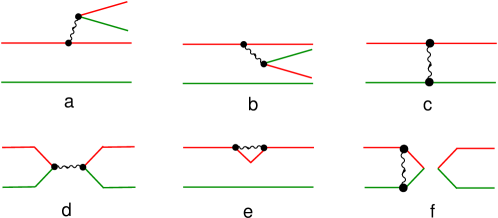
Figure 1: Quark topologies for weak decays; red lines are quarks, green lines are anti-quarks and the wavy line is a $W\,$.

Calculations in non-perturbative QCD are difficult and can only be performed by means of conceptual approximations. A rather powerful approximate scheme relies on the idea that the masses of the light quarks $u\,$, $d\,$, $s$ have just a limited relevance in processes involving low-energy mesons, so that they can be treated perturbatively. In the massless limit, the light sector becomes symmetric under the $SU(3)\times SU(3)$ flavour group associated with chiral symmetry and the approximate scheme is known as chiral perturbation theory (ChPT) [7, 8]. An important feature of this approach is that the light condensates present in the vacuum are properly taken into account and pseudoscalar mesons are collective objects known as Goldstone bosons. The programme is implemented by means of effective lagrangians, which incorporate the symmetries of QCD whereas weak and electromagnetic interactions are included as external sources. The inclusion of heavy mesons can be performed by suitable adaptations of the light sector [9]. At low energies, chiral perturbation theory provides the most precise representation of QCD and unitarization of amplitudes, supplemented by the use of form factors, yields a reliable procedure for encompassing higher energies [10, 11].

3 dynamics

The reaction $D^{+}\rightarrow K^{-}\pi^{+}\pi^{+}$ involves two distinct structures. The first one concerns the primary quark transition $c\rightarrow s\;W^{+}\,$, which occurs in the presence of the light quark condensate of the QCD vacuum and is dressed into hadrons. The second class of processes corresponds to three-body final state interactions (FSIs), associated with the strong propagation of the state produced in the weak vertex to the detector, which eventually identifies a $K^{-}\pi^{+}\pi^{+}$ state. This amounts, in other words, to a kind of hadronic interpolation between decay and detection. These ideas are summarized in Fig.2.

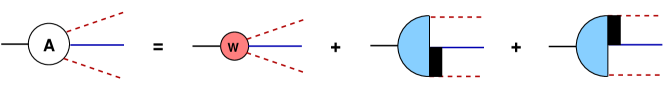
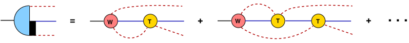
Figure 2: Diagrammatic representation of the heavy meson decay into $K\pi\pi$, starting from the weak amplitude (red) and including hadronic final state interactions.

3.1 weak vertex

The description of the weak vertex involves just tree amplitudes and, in the case of the decay $D^{+}\rightarrow K^{-}\pi^{+}\pi^{+}$, only diagrams $a$ and $b$ of Fig.1 contribute. Here we concentrate just on the former class, which gives rise to the hadronic amplitudes shown in Fig.3. It is important to note that processes on the top involve an axial weak current, whereas the bottom diagram is based on a vector current, since our results hint that the latter dominates. The blob in the diagrams summarizes several hadronic processes which contribute to form factors.

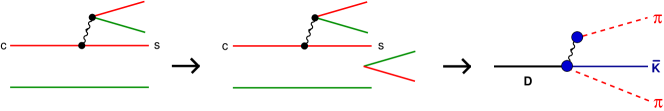
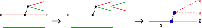
Figure 3: Mechanisms for hadronization; quarks $u$ and $d$ are not specified.

In the absence of form factors, the weak vertex entering Fig.2 is given by the diagrams shown in Fig.4, where processes $a$ and $b$ involve the axial current and $c$ contains a vector current. It is worth noting that one of the pions entering process $c$ is neutral and hence this diagram does not contribute at tree level.

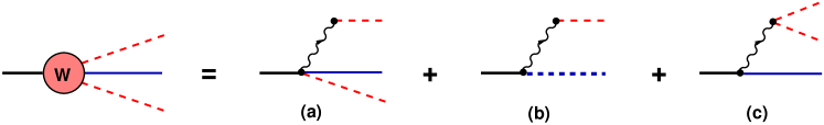
Figure 4: Topologies for the weak vertex: the dotted line is a scalar resonance and the wavy line is a $W^{+}$, which is contracted to a point in calculations.

The inclusion of form factors can be made either by using phenomenological input or by allowing the intermediate propagation of $(c\overline{s})$ states, as shown in Figs.5 and 6.

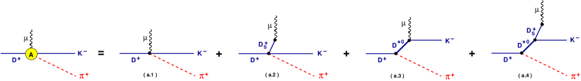
Figure 5: Axial form factor.

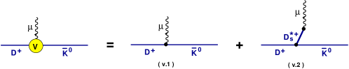
Figure 6: Vector form factor.

3.2 final state interactions

When final state interactions are added to the processes of Fig.4, one finds three families of color-allowed diagrams, as shown in Figs.7-9. The $W^{+}$ is shown explicitly just for the sake of clarifying the various topologies, and is taken as a point in calculations. The class of FSIs considered is based on a succession of elastic two-body interactions, which bring the $K\pi$ phase into the problem. Processes involving resonances have already been considered in Refs.[12, 13] and quasi two-body axial FSIs have been discussed Ref.[14]. In our approach, the construction of the width of the forward propagating resonance[15] is displayed at the bottom of Fig.9. In the sequence, amplitudes corresponding to Figs.7-9 are denoted respectively by $A_{a}\,$, $A_{b}\,$, and $A_{c}\,$.

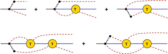
Figure 7: Diagrams starting from the axial weak vertex $W_{a}$; the wavy line is a $W^{+}$, always plugged to a $\pi^{+}$; the $\pi$ produced together with the $\overline{K}$ in the opposite side can be either positive or neutral.

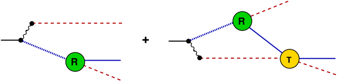
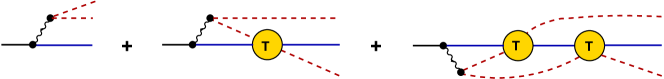
Figure 8: Diagrams starting from the axial vertex $W_{b}$; the wavy line is a $W^{+}$, always plugged to a $\pi^{+}$ and the dotted line is a scalar resonance, which has the width described at the bottom line.

Figure 9: Diagrams starting from the vector vertex $W_{c}$; one of the pions in the weak vertex is neutral.

3.3 elastic $K\pi$ amplitude

The $K\pi$ amplitude required in the construction of three-body FSIs is derived by means of chiral effective lagrangians, based on leading order contact terms [7] and supplemented by resonances [8], which allow for a wider energy range.

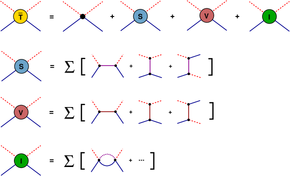
Figure 10: $K\pi$ amplitude: the contact diagram is leading one at low-energies, whereas blobs are corrections due to other intermediate states; $S$ and $V$ correspond to scalar and vector resonances and $I$, to inelastic channels; summation signs indicate the possibility of more than one intermediate state of each kind.

Tree-level interactions, shown in Fig.10, give rise to a kernel ${\cal{K}}\,$. The interaction of ${\cal{K}}\,$ in the Bethe-Salpeter equation[10] yields a unitary elastic amplitude $T\,$, given by

$$T \!=\! {\cal{K}}-{\cal{K}}\,\Omega\,{\cal{K}}+{\cal{K}}\,\Omega\,{\cal{K}}\,\Omega\,{\cal{K}}+\cdots=\frac{{\cal{K}}}{1+\Omega\,{\cal{K}}}\;,$$ (1)

where $\Omega$ is a two-meson propagator, which is a complex function above threshold. Its real component is ultraviolet divergent and requires a subtraction. The corresponding regular part is denoted by $\overline{\Omega}\,$ and can be evaluated analytically. After regularization, eq.(1) becomes

$$T=\frac{{\cal{K}}}{1+[C+\overline{\Omega}]\,{\cal{K}}}\;$$ (2)

where $C$ is a constant adjusted to data.

If one wants, this result can be cast in a Breit-Wigner form, as

$$T=-\frac{16\pi}{\rho}\;\frac{m\;\Gamma}{(s-{\cal{M}}^{2})+i\,m\,\Gamma}\,,$$ (3)

where $\rho=\sqrt{1\!-\!2(M_{\pi}^{2}\!+\!M_{K}^{2})/s\!+\!(M_{\pi}^{2}\!-\!M_{K}^{2})^{2}}\;$, ${\cal{M}}$ is a running mass and $\Gamma$ is a width, which includes suitable kinematic factors. The analytic extension of this amplitude to the second Riemann sheet gives rise to poles. If one does not include explicit resonances into the lagrangian, one gets a single dynamically generated pole. If just one explicit resonance is included, one gets a pair of coupled poles, and so on. This means that eq.(3) always yields a dynamical pole, which is rather broad and, in the $K\pi$ system, is identified as the $\kappa\;$. This picture is consistent with chiral symmetry, since a low-mass resonance cannot be accommodated into effective lagrangians.

An important feature of the dynamical kernel produced by diagrams of Fig.10 is that it vanishes for $\sqrt{s}\sim 1.5\,$GeV$\rightarrow\,s\sim 2.3\,$GeV². This zero propagates into the $K\pi$ amplitude by means of eq.(2), as shown in Fig.11 and therefore becomes a kind of signature of two-body amplitudes in FSIs.

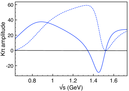
Figure 11: Real (full line) and imaginary (dashed line) components of the $K\pi$ amplitude from eq.(2).

4 first results

In a previous publication [4], we evaluated the contributions of Figs.7-9 to the $S$-wave $[K^{-}\pi^{+}]_{D^{+}}$ sub-amplitude in the decay $D^{+}\rightarrow K^{-}\pi^{+}\pi^{+}$. With the purpose of taming the calculation, we made a number of simplifying assumptions. Among them: the weak amplitudes of Fig.4 were taken to be constants, isospin $3/2$ and $P$ waves were not included in the $K\pi$ amplitude and couplings to either vector mesons or inelastic channels were neglected.

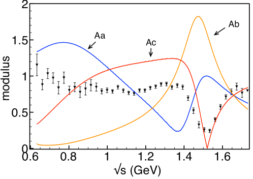
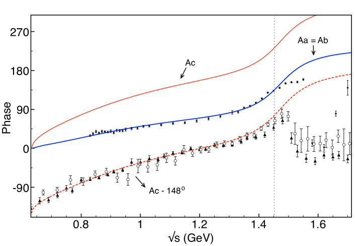
Figure 12: Behaviour of $|A_{a}|$, $|A_{b}|$ and $|A_{c}|$ compared with FOCUS data[2]; scales are arbitrary.

Figure 13: Phase for $A_{a}$, $A_{b}$, $A_{c}$ at leading order and $A_{c}$ shifted by $-148^{0}$ compared with FOCUS [2](triangle) and E791[1](circle) data, together with elastic $K\pi$ results from LASS[3](diamond).

Predictions for the modulus of $[K^{-}\pi^{+}]_{D^{+}}$ are given in Fig.13. Since all tree amplitudes in Fig.4 were assumed to be constants, departures from horizontal straight lines in these figures are signatures of final state interactions. As there is no vector contribution at tree level, one would have $A_{c}=0$ in the absence of FSIs. In the case of amplitudes $A_{a}$ and $A_{c}$, one finds dips around $m_{12}\sim 1.5\,$GeV, whereas $A_{b}$ has a peak in that region. Comparing these predictions with FOCUS data [2], one learns that the dip of the vector contribution $A_{c}$ occurs at the correct position, which is also the point where the elastic $K\pi$ amplitude vanishes, suggesting a direct correlation. On the other hand, compatibility of data with $A_{b}\,$, which represents the direct production of a resonance at the weak vertex, seems to be very difficult.

Results for the phase are displayed in fig.13. Leading order contributions from the axial weak current, represented by $A_{a}$ and $A_{b}\,$, obey Watson’s theorem and fall on top of elastic $K\pi$ data. The curve for the vector $A_{c}$ amplitude has a different shape and, if shifted by $-148^{0}$, can describe well FOCUS data[2], up to the region of the peak.

The main lesson to be drawn from our first approach to this problem is that, for some yet unknown reason, the amplitude which begins with a vector weak current, represented by diagram $(c)$ of Fig.4, seems to be favoured by data. This amplitude receives no contribution at tree level, since the $W^{+}$ emitted by the charmed quark decays into a $\pi^{+}\pi^{0}$ pair. Therefore, the leading term in this kind of process necessarily involves loops and the corresponding imaginary components. This motivates our present attempt to improve the description of the vector vertex, discussed in the next section.

5 vector vertex

A limitation of our first study[4] of the reaction $D^{+}\rightarrow K^{-}\pi^{+}\pi^{+}$ was that all weak vertices were described by momentum independent functions. Those results are now improved by considering: the proper $P$-wave structure of the weak vertex, corrections associated with form factors and contributions from intermediate $\rho$ mesons. Our basic interaction is described in Fig.14.

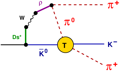
Figure 14: Leading vector contribution.

The $\rho$ is introduced by means of standard vector meson dominance, using the formalism given in Ref.[8]. The $D\rightarrow W\overline{K}$ vertex may contain $(\overline{s}c)$ intermediate states and can be obtained either by means of heavy-meson effective lagrangians[9] and the diagrams of Figs.5-6, or by using phenomenological information parametrized in terms of nearest pole dominance [16]. In the evaluation of fig.14, the $W$ is taken to be very heavy and one is left with four hadronic propagators, which yield finite values for loop integrals.

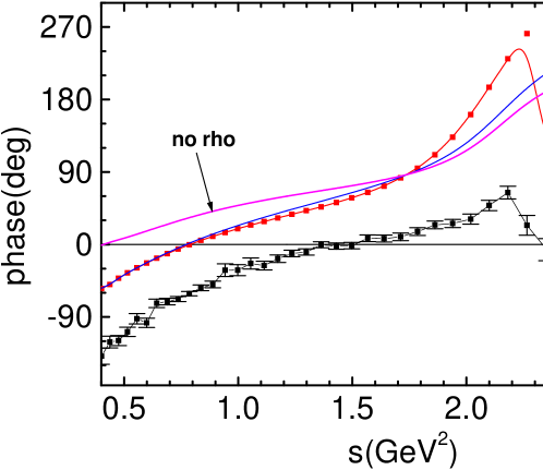
Figure 15: Predictions for the phase, compared with FOCUS results[2].

New predictions for the phase are shown in the red curve of Fig.15. Form factors, as expected, become more important at higher energies, as indicated by the blue “no form factors” curve. The “no rho” magenta curve is obtained by taking the limit $m_{\rho}\rightarrow\infty$ in the calculation and tends to that labelled $A_{c}$ in Fig.13. The most prominent feature of the full phase is that it now has a negative value at threshold, showing that contributions from light intermediate resonances are important. In QCD, loops are the only source of complex amplitudes. As the energy available in the loop of Fig.14 may be larger of both the $K\pi$ and $K\rho$ thresholds, the amplitude has a rich complex structure. So far, the rho has just been treated as a point-like particle. However its width, associated with two-pion intermediate states, is a new source of complex amplitudes and is at present being included into the calculation.

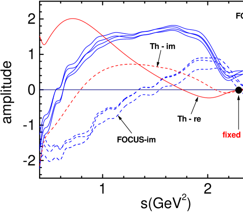
Figure 16: Theoretical amplitude $[K^{-}\pi^{+}]_{D^{+}}$ multiplied by 4 (red) compared with FOCUS [2] data with error bars (blue).

In Fig.16 we display the real and imaginary components of the $S$-wave $[K^{-}\pi^{+}]_{D^{+}}$ amplitude determined by the FOCUS Collaboration [2]. A remarkable feature of these results is that both of them become very small around $s\sim 2.3\,$GeV². This feature is related with the vanishing of the elastic $K\pi$ amplitude, shown in Fig.11, which occurs at the same energy. In fact, around that region and for $S$-waves, both figures suggest that $[K^{-}\pi^{+}]_{D^{+}}$ is proportional to $-i\,T_{K^{-}\pi^{+}}\,$, equation (2). This seems to indicate the presence of loops and therefore to confirm the dominance of weak vector currents in this branch of $D^{+}$ decays. For the sake of completeness, we also show the prediction of the narrow rho to the $[K^{-}\pi^{+}]_{D^{+}}$ amplitude, multiplied by 4, in order to make it more visible.

6 final remarks

We have presented results for the decay $D^{+}\rightarrow K^{-}\pi^{+}\pi^{+}$ and shown that final state interactions are visible in data. Even if our research programme is still incomplete and many aspects of the problem remain to be dealt with, it is already clear that hadronic processes occurring between the primary weak decay and asymptotic propagation to the detector do play a key role in shaping experimental results. Although derived from a single instance, the patterns of hadronic interpolation are quite general and it is fair to assume that this conclusion can be extended to other processes. The treatment of this kind of problem involves many different aspects and is necessarily involved. More theoretical effort on the subject would be definitely welcome [17, 18, 19, 20].

ACKNOWLEDGEMENTS

MRR would like to thanks the organizers of FPCP for the nice and productive conference. PCM was supported by FAPESP, process 09/50634-0.

References

- [1] E.M. Aitala et al. (E791), Phys. Rev. Lett. 89, 121801 (2002).
- [2] J.M. Link et al. [FOCUS Collaboration], Phys. Lett. B 681, (2009) 14;
- [3] D. Aston et al., Nucl.Phys. B 296, 493 (1988); P. Estabrooks et al., Nucl. Phys. B 133, 490 (1978).
- [4] P.C. Magalhães, M.R. Robilotta, K.S.F.F. Guimarães, T. Frederico, W.S. de Paula, I. Bediaga, A.C. dos Reis, and C.M. Maekawa, G.R.S. Zarnauskas, Phys. Rev. D84, 094001 (2011).
- [5] L-L. Chao, Phys. Rep. 95, 1 (1983).
- [6] Bauer, Stich and Wirbel, Z. Phys. C 34, 103 (1987)]
- [7] J. Gasser and H. Leutwyler, Nucl. Phys. B250, 465 (1985); Ann. Phys. 158, 142 (1984).
- [8] G. Ecker, J. Gasser, A. Pich and E. De Rafael, Nucl. Phys. B 321, 311 (1989).
- [9] G. Burdman and J.F. Donoghue, Phys. Lett. B 280, 287 (1992); M.B. Wise, Phys.Rev. D45, R2188 (1992).
- [10] J.A. Oller and E. Oset, Phys. Rev. D 60, 074023 (1999); Nucl. Phys. A 620, 465 (1997); A 652, 407(E) (1999).
- [11] I. Caprini, Phys. Lett. B 638, 468 (2006).
- [12] M. Diakonou and F. Diakonos, Phys. Lett. B 216, 436 (1989)
- [13] H. Kamano, S.X. Nakamura, T.-S.H. Lee and T. Sato, Phys. Rev. D 84, 114019 (2011).
- [14] D. R. Boito, R. Escribano, Phys. Rev. D 80, 054
- [15] D.R. Boito and M.R. Robilotta, Phys. Rev. D 76, 094011 (2007).007 (2009).
- [16] R. Casalbuoni, A. Deandrea, N. Di Bartolomeo, R. Gatto, F. Feruglio and G. Nardulli, Phys.Rep. 281, 145 (1997).
- [17] Bochao Liu, Markus Buescher, Feng-Kun Guo, Christoph Hanhart, and Ulf-G. Meissner, Eur. Phys. J. C 63, 93 (2009).
- [18] Ulf-G. Meissner and Susan Gardner, Eur. Phys. J. A 18, 543 (2003).
- [19] B. Bhattacharya, M Gronau and J.L. Rosner, arXiv[hep-ph 1306.2625] (2013).
- [20] M. Doring,Ulf-G. Mei ner and Wei Wang, arXiv[hep-ph 1307.0947] (2013).