Energy consistent discontinuous Galerkin methods for a quasi-incompressible diffuse two phase flow model

Abstract.

We design consistent discontinuous Galerkin finite element schemes for the approximation of a quasi-incompressible two phase flow model of Allen–Cahn/Cahn–Hilliard/Navier–Stokes–Korteweg type which allows for phase transitions. We show that the scheme is mass conservative and monotonically energy dissipative. In this case the dissipation is isolated to discrete equivalents of those effects already causing dissipation on the continuous level, that is, there is no artificial numerical dissipation added into the scheme. In this sense the methods are consistent with the energy dissipation of the continuous PDE system.

Key words and phrases: Quasi-incompressibility, Allen–Cahn, Cahn–Hilliard, Navier–Stokes–Korteweg, phase transition, energy consistent/mimetic, discontinuous Galerkin finite element method.

1. Introduction

In this work we propose a discontinuous Galerkin (dG) finite element method for a quasi-incompressible phase transition model of Allen–Cahn/Cahn–Hilliard/Navier–Stokes–Korteweg type. These discretisations are of arbitrarily high order in space and provide energy consistent approximations to the model studied. This means the method is automatically endowed with a particular stability property by construction.

Diffuse interface models enjoy the advantage that there is only one set of partial differential equation governing the behaviour of the mixture over the entire domain. Additionally, no particular conditions need be imposed at the interface. Historically, the first diffuse interface model for a mixture of two incompressible Newtonian fluids goes back to the so-called model H proposed in [HH77] where the model is based on the liquids having the same density. In [GPV96, LT98] that model was modified in a thermodynamically consistent way, to allow for liquids with different densities. This situation is known as quasi-incompressibility. While the constituents are incompressible the density of the mixture may vary due to different concentrations of the constituents. In this work we will focus on a model derived in [ADGK] which bears many similarities to [LT98] while it differs in the choice of the energy functional and allows for chemical reactions.

The models mentioned above include a phase field which determines which constituent is present at a certain point, for example, the values $\pm 1$ correspond to the pure constituents. All fields (including the phase field) vary smoothly across the interface between constituents, although steep gradients will usually occur, hence the name diffuse interface model.

The models derived in [LT98, ADGK] enjoy the advantages of being thermodynamically consistent, i.e., they are compatible with an entropy function, which may also serve as a Lyapunov function provided the proper boundary conditions hold, and are frame indifferent. In particular, these models are invariant under Galileian transformations and the only effect of transformations to non-inertial coordinate systems is the introduction of inertial forces, e.g., centrifugal force. On the other hand they have the drawback that they include a complicated constraint for the barycentric (i.e., mass averaged) velocity field, which is no longer solenoidal. Physically this is to be expected in the presence of exchange of mass between both constituents. Given two constituents, A and B, if a certain amount of mass of constituent A becomes constituent B the different densities and the conservation of mass require a change of occupied volume.

The divergence constraint makes the extension of (single phase) incompressible Navier-Stokes solvers infeasible. In addition, the way the Lagrange multiplier accounting for the incompressibility constraints enters the equations in [LT98, ADGK] makes the derivation as well as the numerical analysis of potential schemes challenging. Regardless, in case of [LT98], it is possible to show the model is well-posed, see [Abe09, Abe12]. Although an extension of these results to [ADGK] does not seem to be straightforward and to the best of the knowledge of the authors the well-posedness of (2.9) has not been investigated yet.

The difficulties caused by the divergence constraint have led to the development of models which are built in such a way that the considered (not necessarily barycentric) velocity field is solenoidal, see [AGG12, Boy99, e.g.], which helps the authors of [Grü, GK] in the construction and analysis of a scheme. In particular,

a simplified version of this model [given in [LT98]] has been successfully used for numerical studies …In contrast, there are – to the best of the authors’ knowledge – no discrete schemes available which are based on the full model …This may be due to fundamental new difficulties compared with model H …For instance, the velocity field $\boldsymbol{v}$ is no longer divergence-free and therefore no solution concept is available which avoids …determin[ing] the pressure $p$ [AGG12].

In addition,

Lowengrub and Truskinovsky proposed …for the first time a diffuse-interface model consistent with thermodynamics. The gross velocity field is obtained by mass averaging of individual velocities. As a consequence, it is not divergence free, and the pressure $p$ enters the model as an essential unknown. However, no energy estimates are available to control $p$. Moreover, the pressure enters the chemical potential and is hence strongly coupled to the phase-field equation. This intricate coupling may be one reason why so far it has not been possible to formulate numerical schemes for [the] model [given in [LT98]] [GK].

During the review process of this work, a numerical scheme for the model of Lowengrub–Truskinovsky [LT98] was detailed in [GLL14].

Let us give a short sketch of the derivation of the model in [ADGK]. The authors start from the basic balances for mass, momentum and energy of the mixture. As an isothermal situation is considered the latter is only used to determine the heat flux. The basic balances contain many quantities (e.g. reaction rates, diffusion fluxes, stresses) which need to be modelled by constitutive relations. These are derived by choosing an energy density, introducing a Lagrange multiplier to account for the incompressibility of the constituents and exploiting the requirement of thermodynamical consistency. Sharp interface limits of the model derived in [ADGK] can be found in [ADGK, ADD⁺12]. In particular, the authors show that there is mass transfer across the phase boundary, hence volume of the phases is not conserved.

For the derivation of a viable numerical scheme we use a similar approach to that taken in [GMP13]. Here, the authors designed an approximation of the Navier–Stokes–Korteweg (NSK)/Euler–Korteweg (EK) system to circumvent some of the numerical artefacts which occur when applying “standard” numerical discretisations to the problem. The numerical scheme derived was energy consistent in the sense that for the NSK model it was monotonically energy dissipative and for the EK model it was energy conservative. The underlying idea behind the discretisation was to choose a mixed formulation such that the energy argument at the continuous level could be mimicked at the discrete level. The quasi-incompressible system we address in this work has a similar monotone energy functional as the NSK system (see Theorem 2.6 and [GMP13, Lemma 2.3]). As such, it becomes possible to design the numerical scheme to satisfy a discrete equivalent of this, resulting in a monotonically energy dissipative numerical scheme, without the need for additional artificial dissipation.

Many numerical schemes have been used for the simulation of quasi-incompressible multiphase flows described by sharp interface models. In this approach a lot of care is needed to avoid so called parasitic currents in a vicinity of the interface. They are related to the discretisation of the surface tension forces, [BKZ92, SZ99, VC00, BGN, e.g.]. There is also a considerable amount of numerical schemes based on diffuse interface models for mixtures of two incompressible fluids with differing densities [ALV10, DSS07, DS12, SSO94, ZT07, LS03, SY10, e.g.]

We like to point out that our algorithm does not suffer from parasitic currents, cf. §6.7.

The paper is set out as follows: In §2 we introduce the quasi-incompressible model and some properties, ultimately leading to the introduction of the mixed formulation, which is the basis of designing appropriate numerical schemes. In §3 we detail the construction of a spatially discrete scheme, moving on to the temporally discrete case in §4. We combine the results in §5 to provide a fully discrete scheme. In §6 we conduct various numerical experiments testing convergence in a simple case as well as the energy consistency in one and two spatial dimensions and a test on a rotating coordinate system.

2. Notation and problem setup

In this section we formulate the model problem, fix notation and give some basic assumptions. Let $\Omega\subset\mathbb{R}^{d}$, with $d=1,2,3$ be a bounded domain with Lipschitz boundary. We then begin by introducing the Sobolev spaces [Cia78, Eva98]

(2.1) $$\operatorname{H}^{k}(\Omega):=\left\{\phi\in\operatorname{L}_{2}(\Omega):\;\mathrm{D}^{\boldsymbol{\alpha}}\phi\in\operatorname{L}_{2}(\Omega),\text{ for }\left|\boldsymbol{\alpha}\right|\leq k\right\},$$

which are equipped with norms and semi-norms

(2.2) $$\left\|u\right\|_{k}^{2}:=\left\|u\right\|_{\operatorname{H}^{k}(\Omega)}^{2}=\sum_{\left|\boldsymbol{\alpha}\right|\leq k}\left\|\mathrm{D}^{\boldsymbol{\alpha}}u\right\|_{\operatorname{L}_{2}(\Omega)}^{2}$$

(2.3) $$\text{ and }\left|u\right|_{k}^{2}:=\left|u\right|_{\operatorname{H}^{k}(\Omega)}^{2}=\sum_{\left|\boldsymbol{\alpha}\right|=k}\left\|\mathrm{D}^{\boldsymbol{\alpha}}u\right\|_{\operatorname{L}_{2}(\Omega)}^{2}$$

respectively, where $\boldsymbol{\alpha}=\{\alpha_{1},...,\alpha_{d}\}$ is a multi-index, $\left|\boldsymbol{\alpha}\right|=\sum_{i=1}^{d}\alpha_{i}$ and derivatives $\mathrm{D}^{\boldsymbol{\alpha}}$ are understood in a weak sense. In addition, let

(2.4) $$\operatorname{H}^{1}_{0}:=\left\{\phi\in\operatorname{H}^{1}(\Omega):\;\phi|_{\partial\Omega}=0\right\}\text{ and }\operatorname{H}^{1}_{\boldsymbol{n}}(\Omega):=\left\{\boldsymbol{\phi}\in\!\left[{\operatorname{H}^{1}(\Omega)}\right]^{d}:\;{\left({\boldsymbol{\phi}|_{\partial\Omega}}\right)}^{{\boldsymbol{\intercal}}}\boldsymbol{n}=0\right\}$$

where $\boldsymbol{n}$ denotes the outward pointing normal to $\partial\Omega$.

We use the convention that for a multivariate function, $u$, the quantity $\nabla u$ is a column vector consisting of first order partial derivatives with respect to the spatial coordinates. The divergence operator, $\operatorname{div}{}$, acts on a vector valued multivariate function and $\Delta u:=\operatorname{div}\left({\nabla u}\right)$ is the Laplacian operator. We also note that when the Laplacian acts on a vector valued multivariate function, it is meant componentwise. Moreover, for a vector field $\boldsymbol{v}$, we denote its Jacobian by $\mathrm{D}\boldsymbol{v}$. We also make use of the following notation for time dependant Sobolev (Bochner) spaces:

(2.5) $$\operatorname{L}_{2}(0,T;\operatorname{H}^{k}(\Omega)):=\left\{u:[0,T]\to\operatorname{H}^{k}(\Omega):\;\int_{0}^{T}\left\|u(t)\right\|_{k}^{2}\,\mathrm{d}t<\infty\right\}.$$

2.1. Problem setup

We consider a mixture of two Newtonian fluids, which might be two phases of one substance, or two different substances. As both situations are described by the same model, we will use the terms phase and constituent interchangeably. In the domain $\Omega$ we denote $\phi$ to be the volumetric phase fraction, i.e., it measures the fraction of volume occupied by one of the phases. It is scaled in such a way that $\phi=\pm 1$ corresponds to pure phases. We let $\rho_{1}>0$ and $\rho_{2}>0$ be constants that represent the densities of the incompressible constituents in the fluid. Thus the total density of the mixture is

(2.6) $$\rho(\phi)=\frac{1}{2}\!\left[{\rho_{1}\left({1+\phi}\right)+\rho_{2}\left({1-\phi}\right)}\right].$$

We also introduce the constants

(2.7) $$c_{\pm}:=\frac{1}{\rho_{1}}\pm\frac{1}{\rho_{2}}.$$

We let $\gamma>0$ denote the capillarity constant and $W(\phi)$ be a double well potential of $\phi$ then

(2.8) $$\begin{split}\mu(\phi)&:=W^{\prime}(\phi)-\gamma\Delta\phi\text{ and }\\ p(\phi)&:=\phi W^{\prime}(\phi)-W(\phi)\end{split}$$

represent the chemical potential and pressure respectively. Note that the thickness of the interfacial layer is proportional to $\sqrt{\gamma}$. This can be seen by $\Gamma$-limit techniques, cf. [Ste88, ORS90]. We denote $\boldsymbol{v}$ to be the velocity of the fluid and $\lambda$ is the Lagrange multiplier associated to the incompressibility of the consitutents.

2.2. Quasi-incompressible phase transition model

We then seek $\phi,\boldsymbol{v}\text{ and }\lambda$ such that

(2.9) $$\begin{split}\partial_{t}{\phi}+\operatorname{div}{\phi\boldsymbol{v}}&=c_{+}\left({m_{j}\Delta-m_{r}}\right)\left({c_{+}\mu(\phi)+c_{-}\lambda}\right)\\ \rho(\phi)\left({\partial_{t}{\boldsymbol{v}}+\left({{\boldsymbol{v}}^{{\boldsymbol{\intercal}}}\nabla}\right)\boldsymbol{v}}\right)+\nabla\left({p(\phi)+\lambda}\right)&=\operatorname{div}(\boldsymbol{\sigma}_{NS})+\gamma\phi\nabla\Delta\phi\\ \operatorname{div}{\boldsymbol{v}}&=c_{-}\left({m_{j}\Delta-m_{r}}\right)\left({c_{+}\mu(\phi)+c_{-}\lambda}\right)\end{split}$$

where

(2.10) $$\boldsymbol{\sigma}_{NS}:=\eta_{1}\operatorname{div}\left({\boldsymbol{v}}\right)\boldsymbol{I}_{d}+\eta_{2}\left({\mathrm{D}\boldsymbol{v}+{\left({\mathrm{D}\boldsymbol{v}}\right)}^{{\boldsymbol{\intercal}}}-\frac{2}{d}\operatorname{div}\left({\boldsymbol{v}}\right)\boldsymbol{I}_{d}}\right),$$

is the Navier–Stokes tensor, $\boldsymbol{I}_{d}$ is the $d\times d$ identity matrix and $\eta_{1},\eta_{2}\geq 0$ denote bulk and shear viscosity coefficients and $m_{j},m_{r}>0$ are mobilities. For the derivation of the system (2.9) we refer the reader to [ADGK].

Note, for clarity of exposition we will not use the full Navier–Stokes tensor, but the simplified model:

(2.11) $$\partial_{t}{\phi}+\operatorname{div}\left({\phi\boldsymbol{v}}\right)=c_{+}\left({m_{j}\Delta-m_{r}}\right)\left({c_{+}\mu(\phi)+c_{-}\lambda}\right)$$

(2.12) $$\rho(\phi)\left({\partial_{t}{\boldsymbol{v}}+\left({{\boldsymbol{v}}^{{\boldsymbol{\intercal}}}\nabla}\right)\boldsymbol{v}}\right)+\nabla\left({p(\phi)+\lambda}\right)=\eta\Delta\boldsymbol{v}+\gamma\phi\nabla\Delta\phi$$

(2.13) $$\operatorname{div}\left({\boldsymbol{v}}\right)=c_{-}\left({m_{j}\Delta-m_{r}}\right)\left({c_{+}\mu(\phi)+c_{-}\lambda}\right),$$

with $\eta>0$. An energy consistent discretisation of the full model follows our arguments given a standard (signed) discretisation of the Navier–Stokes tensor and numerical experiments to this end are given in §6.8.

2.3 Remark (local conservation of mass).

It is important to observe that combining (2.11) and (2.13) gives

(2.14) $$\frac{c_{-}}{c_{+}}\left({\partial_{t}{\phi}+\operatorname{div}\left({\phi\boldsymbol{v}}\right)}\right)-\operatorname{div}{\boldsymbol{v}}=0.$$

Due to (2.6) and (2.7) this is equivalent to

(2.15) $$\partial_{t}{\rho}(\phi)+\operatorname{div}(\rho(\phi)\boldsymbol{v})=0,$$

i.e., the (local) conservation of mass is encoded in (2.11)–(2.13).

2.4 Remark (boundary conditions).

We associate with (2.11)–(2.13) the following boundary conditions:

(2.16) $$\nabla\phi\cdot\boldsymbol{n}=0$$

(2.17) $$\boldsymbol{v}=\boldsymbol{0}$$

(2.18) $$\left({\nabla\left({c_{+}\mu(\phi)+c_{-}\lambda}\right)}\right)\cdot\boldsymbol{n}=0.$$

This choice yields global conservation of mass, global momentum balance and a entropy dissipation equality as we will see subsequently.

2.5 Proposition (Conservation of mass,balance of momentum).

Let $\left({\phi,\boldsymbol{v},\lambda}\right)$ be a strong solution to the system (2.11)–(2.13) satisfying the boundary conditions in Remark 2.4 then

(2.19) $$\,\mathrm{d}_{t}\left({\int_{\Omega}\rho(\phi)}\right)=0,$$

and

(2.20) $$\,\mathrm{d}_{t}\left({\int_{\Omega}\rho(\phi)\boldsymbol{v}}\right)=-\int_{\partial\Omega}\left({p(\phi)+\lambda-\phi\Delta\phi}\right)\boldsymbol{n}-\left({D\boldsymbol{v}}\right)\cdot\boldsymbol{n}.$$

Proof The proof of (2.19) can be seen using Remark 2.3 and the boundary conditions (2.17). To see (2.20) it is enough to use (2.12), the identity

(2.21) $$\phi\nabla\Delta\phi=\operatorname{div}\left({\left({\phi\Delta\phi+\frac{1}{2}\left|\nabla\phi\right|^{2}}\right)\boldsymbol{I}_{d}-\nabla\phi\otimes\nabla\phi}\right),$$

and the boundary conditions. ∎

For completeness we formulate the energy dissipation equality in Theorem 2.6. Its validity is a direct consequence of the modeling paradigm employed in [ADGK] and a proof can be found in [ADD⁺12]. We have organized the proof in such a way that it may serve as a guideline for the construction of a numerical discretisation which satisfies a discrete energy dissipation equality.

2.6 Theorem (energy dissipation equality).

Let $\left({\phi,\boldsymbol{v},\lambda}\right)$ be a strong solution to the system (2.11)–(2.13) satisfying the boundary conditions in Remark 2.4, then

(2.22) $$\begin{split}\,\mathrm{d}_{t}\left({\int_{\Omega}W(\phi)+\frac{\rho(\phi)}{2}\left|\boldsymbol{v}\right|^{2}+\frac{\gamma}{2}\left|\nabla\phi\right|^{2}}\right)=-\int_{\Omega}m_{j}&\left|\nabla\left({c_{+}\mu(\phi)+c_{-}\lambda}\right)\right|^{2}\\ &+m_{r}\left({c_{+}\mu(\phi)+c_{-}\lambda}\right)^{2}+\eta\left|\mathrm{D}\boldsymbol{v}\right|^{2}.\end{split}$$

Proof Let

(2.23) $$\begin{split}a&=c_{+}\mu(\phi)+c_{-}\lambda\text{ and }\\ b&=\lambda+\frac{\rho_{1}+\rho_{2}}{4}\left|\boldsymbol{v}\right|^{2}.\end{split}$$

We proceed by testing (2.11) with $\frac{a}{c_{+}}$ and (2.12) with $\boldsymbol{v}$ and taking the sum, yielding

(2.24) $$\begin{split}0&=\int_{\Omega}\frac{a\partial_{t}{\phi}}{c_{+}}+\frac{a\operatorname{div}\left({\phi\boldsymbol{v}}\right)}{c_{+}}-m_{j}a\Delta a+m_{r}a^{2}+\rho(\phi)\bigg{(}\partial_{t}{\boldsymbol{v}}\cdot\boldsymbol{v}+\left({\left({\boldsymbol{v}\cdot\nabla}\right)\boldsymbol{v}}\right)\cdot\boldsymbol{v}\\ &\qquad\qquad-\frac{1}{2}\nabla\left({\left|\boldsymbol{v}\right|^{2}}\right)\cdot\boldsymbol{v}\bigg{)}+\nabla b\cdot\boldsymbol{v}+\frac{\phi}{c_{+}}\nabla\left({a-c_{-}b}\right)\cdot\boldsymbol{v}-\eta\boldsymbol{v}\cdot\Delta\boldsymbol{v}.\end{split}$$

Integrating by parts and noting that

(2.25) $$\left({\left({\boldsymbol{v}\cdot\nabla}\right)\boldsymbol{v}}\right)\cdot\boldsymbol{v}-\frac{1}{2}\nabla\left({\left|\boldsymbol{v}\right|^{2}}\right)\cdot\boldsymbol{v}=0$$

gives

(2.26) $$\begin{split}0&=\int_{\Omega}\frac{a\partial_{t}{\phi}}{c_{+}}+\frac{a\operatorname{div}\left({\phi\boldsymbol{v}}\right)}{c_{+}}+m_{j}\left|\nabla a\right|^{2}+m_{r}a^{2}+\rho(\phi)\partial_{t}{\boldsymbol{v}}\cdot\boldsymbol{v}+\nabla b\cdot\boldsymbol{v}\\ &\qquad\qquad+\frac{\phi}{c_{+}}\nabla\left({a-c_{-}b}\right)\cdot\boldsymbol{v}+\eta\left|\mathrm{D}\boldsymbol{v}\right|^{2}-\int_{\partial\Omega}m_{j}a\nabla a\cdot\boldsymbol{n}+\eta\left({\mathrm{D}\boldsymbol{v}\cdot\boldsymbol{n}}\right)\cdot\boldsymbol{v}.\end{split}$$

Due to the boundary conditions given in Remark 2.4 the boundary terms are zero. In addition we note that

(2.27) $$\int_{\Omega}\frac{a\operatorname{div}\left({\phi\boldsymbol{v}}\right)}{c_{+}}+\frac{\phi\nabla a\cdot\boldsymbol{v}}{c_{+}}=\int_{\Omega}\frac{\operatorname{div}\left({a\phi\boldsymbol{v}}\right)}{c_{+}}=\int_{\partial\Omega}\frac{a\phi\boldsymbol{v}\cdot\boldsymbol{n}}{c_{+}}=0$$

again due to the boundary conditions, leaving

(2.28) $$\begin{split}0&=\int_{\Omega}\frac{a\partial_{t}{\phi}}{c_{+}}+m_{j}\left|\nabla a\right|^{2}+m_{r}a^{2}+\rho(\phi)\partial_{t}{\boldsymbol{v}}\cdot\boldsymbol{v}+\nabla b\cdot\boldsymbol{v}-\frac{c_{-}\phi}{c_{+}}\nabla b\cdot\boldsymbol{v}+\eta\left|\mathrm{D}\boldsymbol{v}\right|^{2}.\end{split}$$

Using the definition of $a$ in the first term and integrating by parts the two terms involving $b$, we see

(2.29) $$\begin{split}0&=\int_{\Omega}W^{\prime}(\phi)\partial_{t}{\phi}-\gamma\partial_{t}{\phi}\Delta\phi+\frac{c_{-}\lambda\partial_{t}{\phi}}{c_{+}}+m_{j}\left|\nabla a\right|^{2}+m_{r}a^{2}+\rho(\phi)\partial_{t}{\boldsymbol{v}}\cdot\boldsymbol{v}\\ &\qquad\qquad-b\operatorname{div}\left({\boldsymbol{v}}\right)+\frac{c_{-}b}{c_{+}}\operatorname{div}\left({\phi\boldsymbol{v}}\right)+\eta\left|\mathrm{D}\boldsymbol{v}\right|^{2}+\int_{\partial\Omega}b\boldsymbol{v}\cdot\boldsymbol{n}-\frac{c_{-}b\phi}{c_{+}}\boldsymbol{v}\cdot\boldsymbol{n}.\end{split}$$

The boundary terms vanish, again, due to Remark 2.4. Using the local conservation of mass (2.14)

(2.30) $$\begin{split}0&=\int_{\Omega}W^{\prime}(\phi)\partial_{t}{\phi}-\gamma\partial_{t}{\phi}\Delta\phi+\frac{c_{-}\lambda\partial_{t}{\phi}}{c_{+}}+m_{j}\left|\nabla a\right|^{2}+m_{r}a^{2}+\rho(\phi)\partial_{t}{\boldsymbol{v}}\cdot\boldsymbol{v}\\ &\qquad\qquad-\frac{c_{-}}{c_{+}}b\partial_{t}{\phi}+\eta\left|\mathrm{D}\boldsymbol{v}\right|^{2}.\end{split}$$

Using the definition of $b$ and integrating the second term by parts, it holds that

(2.31) $$\begin{split}0&=\int_{\Omega}W^{\prime}(\phi)\partial_{t}{\phi}+\gamma\nabla\left({\partial_{t}{\phi}}\right)\nabla\phi+m_{j}\left|\nabla a\right|^{2}+m_{r}a^{2}+\rho(\phi)\partial_{t}{\boldsymbol{v}}\cdot\boldsymbol{v}\\ &\qquad\qquad-\frac{c_{-}\left({\rho_{1}+\rho_{2}}\right)}{4c_{+}}\left|\boldsymbol{v}\right|^{2}\partial_{t}{\phi}+\eta\left|\mathrm{D}\boldsymbol{v}\right|^{2}-\int_{\partial\Omega}\gamma\partial_{t}{\phi}\nabla\phi\cdot\boldsymbol{n}.\end{split}$$

Due to the definition of $c_{\pm}$ (2.7)

(2.32) $$\frac{c_{-}\left({\rho_{1}+\rho_{2}}\right)}{4c_{+}}=\frac{\rho_{2}-\rho_{1}}{4}=-\frac{d\rho(\phi)}{d\phi},$$

and hence

(2.33) $$\begin{split}\int_{\Omega}\,\mathrm{d}_{t}\left({W(\phi)+\frac{\rho(\phi)}{2}\left|\boldsymbol{v}\right|^{2}+\frac{\gamma}{2}\left|\nabla\phi\right|^{2}}\right)&=\int_{\Omega}W^{\prime}(\phi)\partial_{t}{\phi}+\rho(\phi)\partial_{t}{\boldsymbol{v}}\cdot\boldsymbol{v}\\ &\qquad+\frac{c_{-}\left({\rho_{1}+\rho_{2}}\right)}{4c_{+}}\left|\boldsymbol{v}\right|^{2}\partial_{t}{\phi}+\gamma\nabla\left({\partial_{t}{\phi}}\right)\cdot\nabla\phi.\end{split}$$

Using the boundary conditions in Remark 2.4 one final time to eliminate the boundary contributions from (2.31) shows

(2.34) $$0=\int_{\Omega}\,\mathrm{d}_{t}\left({W(\phi)+\frac{1}{2}\rho(\phi)\left|\boldsymbol{v}\right|^{2}+\frac{\gamma}{2}\left|\nabla\phi\right|^{2}}\right)+m_{j}\left|\nabla a\right|^{2}+m_{r}a^{2}+\eta\left|\mathrm{D}\boldsymbol{v}\right|^{2}.$$

The result then follows using the definition of $a$, concluding the proof. ∎

2.7. Continuous mixed formulation

The proof of Theorem 2.6 motivates the introduction of the auxiliary variables $a,b,\boldsymbol{q}$, transforming (2.11)–(2.13) into the following mixed system:

(2.35) $$\begin{split}0&=\partial_{t}{\phi}+\operatorname{div}\left({\phi\boldsymbol{v}}\right)-c_{+}m_{j}\Delta a+c_{+}m_{r}a\\ 0&=\rho(\phi)\left({\partial_{t}{}\boldsymbol{v}+\left({{\boldsymbol{v}}\cdot\nabla}\right)\boldsymbol{v}-\frac{1}{2}\nabla\left({\left|\boldsymbol{v}\right|^{2}}\right)}\right)-\eta\Delta\boldsymbol{v}+\nabla b+\frac{\phi}{c_{+}}\nabla(a-{c_{-}}b)\\ 0&=\operatorname{div}\left({\boldsymbol{v}}\right)-\frac{c_{-}}{c_{+}}\left({\partial_{t}{}\phi+\operatorname{div}\left({\phi\boldsymbol{v}}\right)}\right)\\ 0&=a-c_{+}W^{\prime}(\phi)+c_{+}\gamma\operatorname{div}\left({\boldsymbol{q}}\right)-c_{-}\lambda\\ 0&=b-\lambda-\frac{\rho_{1}+\rho_{2}}{4}\left|\boldsymbol{v}\right|^{2}\\ 0&=\boldsymbol{q}-\nabla\phi,\end{split}$$

coupled with boundary conditions

(2.36) $$\boldsymbol{q}\cdot\boldsymbol{n}=0,\quad\boldsymbol{v}=\boldsymbol{0},\quad\nabla a\cdot\boldsymbol{n}=0.$$

3. Spatially discrete approximation

In this section we design spatially discrete approximations of the system (2.11)–(2.13) of arbitrary order using discontinuous Galerkin finite elements.

Let $\mathscr{T}$ be a conforming, shape regular triangulation of $\Omega$, namely, $\mathscr{T}$ is a finite family of sets such that

1. $K\in\mathscr{T}$ implies $K$ is an open simplex (segment for $d=1$, triangle for $d=2$, tetrahedron for $d=3$),

2. for any $K,J\in\mathscr{T}$ we have that $\overline{K}\cap\overline{J}$ is a full subsimplex (i.e., it is either $\emptyset$, a vertex, an edge, a face, or the whole of $\overline{K}$ and $\overline{J}$) of both $\overline{K}$ and $\overline{J}$ and

3. $\bigcup_{K\in\mathscr{T}}\overline{K}=\overline{\Omega}$.

We use the convention where $h:\Omega\to\mathbb{R}$ denotes the meshsize function of $\mathscr{T}$, i.e.,

(3.1) $$h(\boldsymbol{x}):=\max_{\overline{K}\ni\boldsymbol{x}}h_{K},$$

where $h_{K}$ is the diameter of an element $K$. We let $\mathscr{E}{}$ be the skeleton (set of common interfaces) of the triangulation $\mathscr{T}$ and say $e\in\mathscr{E}$ if $e$ is on the interior of $\Omega$ and $e\in\partial\Omega$ if $e$ lies on the boundary $\partial\Omega$.

3.1 Definition (broken Sobolev spaces, trace spaces).

We introduce the broken Sobolev space

(3.2) $$\operatorname{H}^{k}(\mathscr{T}):=\left\{\phi:\;\phi|_{K}\in\operatorname{H}^{k}(K),\text{ for each }K\in\mathscr{T}\right\},$$

similarly for $\operatorname{H}^{1}_{0}(\mathscr{T})$ and $\operatorname{H}^{1}_{\boldsymbol{n}}(\mathscr{T})$.

We also make use of functions defined in these broken spaces restricted to the skeleton of the triagulation. This requires an appropriate trace space

(3.3) $$\mathcal{T}\left({\mathscr{E}}\right):=\prod_{K\in\mathscr{T}}\operatorname{L}_{2}(\partial K)\subset\prod_{K\in\mathscr{T}}\operatorname{H}^{\frac{1}{2}}(K).$$

Let $\mathbb{P}^{p}(\mathscr{T})$ denote the space of piecewise polynomials of degree $p$ over the triangulation $\mathscr{T}$ we then introduce the finite element spaces

(3.4) $$\mathbb{V}:=\mathbb{D}\mathbb{G}({\mathscr{T}},{p})=\mathbb{P}^{p}(\mathscr{T})$$

(3.5) $$\accentset{\circ}{\mathbb{V}}:=\mathbb{V}\cap\operatorname{H}^{1}_{0}(\mathscr{T})$$

(3.6) $$\accentset{\boldsymbol{n}}{\mathbb{V}}:=\mathbb{V}^{d}\cap\operatorname{H}^{1}_{\boldsymbol{n}}(\mathscr{T})$$

to be the usual spaces of (discontinuous) piecewise polynomial functions. For simplicity we will assume that $\mathbb{V}$ is constant in time.

3.2 Definition (jumps and averages).

We may define average and jump operators over $\mathcal{T}\left({\mathscr{E}}\right)$ for arbitrary scalar, $v\in\mathcal{T}\left({\mathscr{E}}\right)$, and vector valued functions, $\boldsymbol{v}\in\mathcal{T}\left({\mathscr{E}}\right)^{d}$.

(3.7) $$\begin{array}[]{rccl}{\mathrel{\ooalign{\cr\kern 1.0pt$\{$\cr\kern-0.5pt$\{$}}\cdot\mathrel{\ooalign{$\}$\cr\kern-1.5pt$\}$\cr\kern-1.0pt}}}:&{\mathcal{T}\left({\mathscr{E}\cup\partial\Omega}\right)}&\to&{\operatorname{L}_{2}(\mathscr{E}\cup\partial\Omega)}\\ &{v}&\mapsto&{\frac{1}{2}\left({v|_{K_{1}}+v|_{K_{2}}}\right).}\end{array}\quad$$

(3.8) $$\begin{array}[]{rccl}{\mathrel{\ooalign{\cr\kern 1.0pt$\{$\cr\kern-0.5pt$\{$}}\cdot\mathrel{\ooalign{$\}$\cr\kern-1.5pt$\}$\cr\kern-1.0pt}}}:&{\left({\mathcal{T}\left({\mathscr{E}\cup\partial\Omega}\right)}\right)^{d}}&\to&{\left({\operatorname{L}_{2}(\mathscr{E}\cup\partial\Omega)}\right)^{d}}\\ &{\boldsymbol{v}}&\mapsto&{\frac{1}{2}\left({\boldsymbol{v}|_{K_{1}}+\boldsymbol{v}|_{K_{2}}}\right).}\end{array}\quad$$

(3.9) $$\begin{array}[]{rccl}{\left\llbracket\cdot\right\rrbracket}:&{\mathcal{T}\left({\mathscr{E}\cup\partial\Omega}\right)}&\to&{\left({\operatorname{L}_{2}(\mathscr{E}\cup\partial\Omega)}\right)^{d}}\\ &{v}&\mapsto&{{{v}|_{K_{1}}\boldsymbol{n}_{K_{1}}+{v}|_{K_{2}}}\boldsymbol{n}_{K_{2}}.}\end{array}\quad$$

(3.10) $$\begin{array}[]{rccl}{\left\llbracket\cdot\right\rrbracket}:&{\left({\mathcal{T}\left({\mathscr{E}\cup\partial\Omega}\right)}\right)^{d}}&\to&{\operatorname{L}_{2}(\mathscr{E}\cup\partial\Omega)}\\ &{\boldsymbol{v}}&\mapsto&{{{\left({\boldsymbol{v}|_{K_{1}}}\right)}^{{\boldsymbol{\intercal}}}\boldsymbol{n}_{K_{1}}+{\left({\boldsymbol{v}|_{K_{2}}}\right)}^{{\boldsymbol{\intercal}}}\boldsymbol{n}_{K_{2}}}.}\end{array}\quad$$

(3.11) $$\begin{array}[]{rccl}{\left\llbracket\cdot\right\rrbracket_{\otimes}}:&{\left({\mathcal{T}\left({\mathscr{E}\cup\partial\Omega}\right)}\right)^{d}}&\to&{\left({\operatorname{L}_{2}(\mathscr{E}\cup\partial\Omega)}\right)^{d\times d}}\\ &{\boldsymbol{v}}&\mapsto&{{\boldsymbol{v}|_{K_{1}}}\otimes\boldsymbol{n}_{K_{1}}+\boldsymbol{v}|_{K_{2}}\otimes\boldsymbol{n}_{K_{2}},}\end{array}\quad$$

where $\boldsymbol{n}_{K_{i}}$ denotes the outward pointing normal to $K_{i}$. Note that on the boundary of the domain $\partial\Omega$ the jump and average operators are defined as

(3.12) $$\left\llbracket v\right\rrbracket\Big{|}_{\partial\Omega}:=v\boldsymbol{n}\qquad\left\llbracket\boldsymbol{v}\right\rrbracket\Big{|}_{\partial\Omega}:={\boldsymbol{v}}^{{\boldsymbol{\intercal}}}\boldsymbol{n}\qquad\left\llbracket\boldsymbol{v}\right\rrbracket_{\otimes}\Big{|}_{\partial\Omega}:=\boldsymbol{v}\otimes\boldsymbol{n}$$

(3.25) $$\mathrel{\ooalign{\cr\kern 1.0pt$\{$\cr\kern-0.5pt$\{$}}v\mathrel{\ooalign{$\}$\cr\kern-1.5pt$\}$\cr\kern-1.0pt}}\Big{|}_{\partial\Omega}:=v\qquad\mathrel{\ooalign{\cr\kern 1.0pt$\{$\cr\kern-0.5pt$\{$}}\boldsymbol{v}\mathrel{\ooalign{$\}$\cr\kern-1.5pt$\}$\cr\kern-1.0pt}}\Big{|}_{\partial\Omega}:=\boldsymbol{v}.$$

3.3. Discrete mixed formulation

We propose the following semidiscrete (spatially discrete) formulation of the system: To find $\big{(}\phi_{h}$, $\boldsymbol{v}_{h}$, $\lambda_{h}$, $a_{h}$, $b_{h}$, $\boldsymbol{q}_{h}\big{)}\in C^{1}([0,T),\mathbb{V})\times C^{1}([0,T),\accentset{\circ}{\mathbb{V}}^{d})\times C^{0}([0,T),\mathbb{V})\times C^{0}([0,T),\mathbb{V})\times C^{0}([0,T),\mathbb{V})\times C^{0}([0,T),\accentset{\boldsymbol{n}}{\mathbb{V}})$ such that

(3.26) $$\begin{split}0&=\int_{\Omega}\left({\partial_{t}{}\phi_{h}+\operatorname{div}\left({\phi_{h}\boldsymbol{v}_{h}}\right)+c_{+}m_{r}a_{h}}\right)\mathrm{X}-c_{+}m_{j}\mathscr{A}_{1}(a_{h},\mathrm{X})-\int_{\mathscr{E}}\left\llbracket\phi_{h}\boldsymbol{v}_{h}\right\rrbracket\mathrel{\ooalign{\cr\kern 1.0pt$\{$\cr\kern-0.5pt$\{$}}\mathrm{X}\mathrel{\ooalign{$\}$\cr\kern-1.5pt$\}$\cr\kern-1.0pt}}\\ 0&=\int_{\Omega}\rho(\phi_{h})\partial_{t}{}\boldsymbol{v}_{h}\cdot\boldsymbol{\Xi}+\rho(\phi_{h})\left({\left({\boldsymbol{v}_{h}\cdot\nabla}\right)\boldsymbol{v}_{h}}\right)\cdot\boldsymbol{\Xi}\\ &\qquad\qquad-\frac{1}{2}\rho(\phi_{h})\nabla\left({\left|\boldsymbol{v}_{h}\right|^{2}}\right)\cdot\boldsymbol{\Xi}+\nabla b_{h}\cdot\boldsymbol{\Xi}+\frac{\phi_{h}}{c_{+}}\nabla(a_{h}-c_{-}b_{h})\cdot\boldsymbol{\Xi}-\eta\mathscr{A}_{2}\left({{\boldsymbol{v}_{h}},{\boldsymbol{\Xi}}}\right)\\ &\qquad+\int_{\mathscr{E}}\left({{-}\mathrel{\ooalign{\cr\kern 1.0pt$\{$\cr\kern-0.5pt$\{$}}\boldsymbol{\Xi}\mathrel{\ooalign{$\}$\cr\kern-1.5pt$\}$\cr\kern-1.0pt}}\otimes\mathrel{\ooalign{\cr\kern 1.0pt$\{$\cr\kern-0.5pt$\{$}}\rho(\phi_{h})\boldsymbol{v}_{h}\mathrel{\ooalign{$\}$\cr\kern-1.5pt$\}$\cr\kern-1.0pt}}}\right):\left\llbracket\boldsymbol{v}_{h}\right\rrbracket_{\otimes}{+}\frac{1}{2}\left\llbracket\left|\boldsymbol{v}_{h}\right|^{2}\right\rrbracket\cdot\mathrel{\ooalign{\cr\kern 1.0pt$\{$\cr\kern-0.5pt$\{$}}\rho(\phi_{h})\boldsymbol{\Xi}\mathrel{\ooalign{$\}$\cr\kern-1.5pt$\}$\cr\kern-1.0pt}}\\ &\qquad\qquad-\left\llbracket b_{h}\right\rrbracket\cdot\mathrel{\ooalign{\cr\kern 1.0pt$\{$\cr\kern-0.5pt$\{$}}\boldsymbol{\Xi}\mathrel{\ooalign{$\}$\cr\kern-1.5pt$\}$\cr\kern-1.0pt}}-\frac{1}{c_{+}}\left\llbracket a_{h}-c_{-}b_{h}\right\rrbracket\cdot\mathrel{\ooalign{\cr\kern 1.0pt$\{$\cr\kern-0.5pt$\{$}}\phi_{h}\boldsymbol{\Xi}\mathrel{\ooalign{$\}$\cr\kern-1.5pt$\}$\cr\kern-1.0pt}}\\ 0&=\int_{\Omega}\operatorname{div}\left({\boldsymbol{v}_{h}}\right)\mathrm{Z}-\frac{c_{-}}{c_{+}}\partial_{t}{}\phi_{h}\mathrm{Z}-\frac{c_{-}}{c_{+}}\operatorname{div}\left({\phi_{h}\boldsymbol{v}_{h}}\right)\mathrm{Z}+\int_{\mathscr{E}}\left\llbracket\frac{c_{-}}{c_{+}}\phi_{h}\boldsymbol{v}_{h}-\boldsymbol{v}_{h}\right\rrbracket\mathrel{\ooalign{\cr\kern 1.0pt$\{$\cr\kern-0.5pt$\{$}}\mathrm{Z}\mathrel{\ooalign{$\}$\cr\kern-1.5pt$\}$\cr\kern-1.0pt}}\\ 0&=\int_{\Omega}\left({a_{h}-c_{+}W^{\prime}(\phi_{h})-c_{-}\lambda_{h}}\right)\Psi+c_{+}\gamma\operatorname{div}\left({\boldsymbol{q}_{h}}\right)\Psi-c_{+}\gamma\int_{\mathscr{E}}\left\llbracket\boldsymbol{q}_{h}\right\rrbracket\mathrel{\ooalign{\cr\kern 1.0pt$\{$\cr\kern-0.5pt$\{$}}\Psi\mathrel{\ooalign{$\}$\cr\kern-1.5pt$\}$\cr\kern-1.0pt}}\\ 0&=\int_{\Omega}\left({b_{h}-\lambda_{h}-\frac{\rho_{1}+\rho_{2}}{4}\left|\boldsymbol{v}_{h}\right|^{2}}\right)\Upsilon\\ 0&=\int_{\Omega}\boldsymbol{q}_{h}\cdot\boldsymbol{\mathrm{T}}-\nabla\phi_{h}\cdot\boldsymbol{\mathrm{T}}+\int_{\mathscr{E}}\left\llbracket\phi_{h}\right\rrbracket\cdot\mathrel{\ooalign{\cr\kern 1.0pt$\{$\cr\kern-0.5pt$\{$}}\boldsymbol{\mathrm{T}}\mathrel{\ooalign{$\}$\cr\kern-1.5pt$\}$\cr\kern-1.0pt}}\\ &\qquad\qquad\quad\>\forall\>\left({\mathrm{X},\boldsymbol{\Xi},\mathrm{Z},\Psi,\Upsilon,\boldsymbol{\mathrm{T}}}\right){\in\mathbb{V}\times\accentset{\circ}{\mathbb{V}}^{d}\times\mathbb{V}\times\mathbb{V}\times\mathbb{V}\times\accentset{\boldsymbol{n}}{\mathbb{V}}.}\end{split}$$

Where

(3.27) $$\begin{split}\mathscr{A}_{1}\left({a_{h},\mathrm{X}}\right)&=-\int_{\Omega}\nabla a_{h}\cdot\nabla\mathrm{X}+\int_{\mathscr{E}}\mathrel{\ooalign{\cr\kern 1.0pt$\{$\cr\kern-0.5pt$\{$}}\nabla\mathrm{X}\mathrel{\ooalign{$\}$\cr\kern-1.5pt$\}$\cr\kern-1.0pt}}\cdot\left\llbracket a_{h}\right\rrbracket\\ &\qquad+\int_{\mathscr{E}}\left\llbracket\mathrm{X}\right\rrbracket\cdot\mathrel{\ooalign{\cr\kern 1.0pt$\{$\cr\kern-0.5pt$\{$}}\nabla a_{h}\mathrel{\ooalign{$\}$\cr\kern-1.5pt$\}$\cr\kern-1.0pt}}-\frac{\sigma}{h}\left\llbracket a_{h}\right\rrbracket\cdot\left\llbracket\mathrm{X}\right\rrbracket\\ \mathscr{A}_{2}\left({\boldsymbol{v}_{h},\boldsymbol{\Xi}}\right)&=-\int_{\Omega}{\mathrm{D}\boldsymbol{v}_{h}}{:}{\mathrm{D}\boldsymbol{\Xi}}+\int_{\mathscr{E}\cup\partial\Omega}{\mathrel{\ooalign{\cr\kern 1.0pt$\{$\cr\kern-0.5pt$\{$}}\mathrm{D}\boldsymbol{\Xi}\mathrel{\ooalign{$\}$\cr\kern-1.5pt$\}$\cr\kern-1.0pt}}}{:}{\left\llbracket\boldsymbol{v}_{h}\right\rrbracket_{\otimes}}\\ &\qquad+\int_{\mathscr{E}\cup\partial\Omega}{\mathrel{\ooalign{\cr\kern 1.0pt$\{$\cr\kern-0.5pt$\{$}}\mathrm{D}\boldsymbol{v}_{h}\mathrel{\ooalign{$\}$\cr\kern-1.5pt$\}$\cr\kern-1.0pt}}}{:}{\left\llbracket\boldsymbol{\Xi}\right\rrbracket_{\otimes}}-\frac{\sigma}{h}{\left\llbracket\boldsymbol{v}_{h}\right\rrbracket_{\otimes}}{:}{\left\llbracket\boldsymbol{\Xi}\right\rrbracket_{\otimes}}\end{split}$$

represent symmetric interior penalty discretisations of the scalar and vector valued Laplacians respectively, which are signed (coercive) when the penalty parameter $\sigma$ is chosen sufficiently large.

3.4 Remark (discrete boundary conditions).

The boundary conditions (2.36) are encoded in the finite element spaces for the Dirichlet type conditions on $\boldsymbol{v}_{h}$ and $\boldsymbol{q}_{h}$. For $a_{h}$ the Neumann condition is encoded in the bilinear form $\mathscr{A}_{1}$.

3.5 Remark (alternative bilinear forms).

We may choose $\mathscr{A}_{1,2}$ to be any discretisation of scalar and vector valued Laplacian, the only requirement is that they are coercive.

Throughout the calculations in this section we will regularly refer to the following proposition.

3.6 Proposition (elementwise integration).

Let

(3.28) $$\operatorname{H}^{\operatorname{div}}(\mathscr{T}):=\left\{\boldsymbol{p}\in(\operatorname{L}_{2}(\mathscr{T}))^{d}:\;\operatorname{div}\left({\boldsymbol{p}|_{K}}\right)\in\operatorname{L}_{2}(K)\text{ for each }K\in\mathscr{T}\right\}.$$

Suppose $\boldsymbol{p}\in\operatorname{H}^{\operatorname{div}}(\mathscr{T})$ and $\varphi\in\operatorname{H}^{1}(\mathscr{T})$ then

(3.29) $$\begin{split}\sum_{K\in\mathscr{T}}\int_{K}\operatorname{div}\left({\boldsymbol{p}}\right)\varphi\,\mathrm{d}\boldsymbol{x}=\sum_{K\in\mathscr{T}}\left({-\int_{K}\boldsymbol{p}\cdot\nabla\varphi\,\mathrm{d}\boldsymbol{x}+\int_{\partial K}\varphi\boldsymbol{p}\cdot\boldsymbol{n}_{K}\,\mathrm{d}s}\right).\end{split}$$

In particular we have $\boldsymbol{p}\in\mathcal{T}\left({\mathscr{E}}\right)^{d}$ and $\varphi\in\mathcal{T}\left({\mathscr{E}}\right)$, and the following identity holds

(3.30) $$\sum_{K\in\mathscr{T}}\int_{\partial K}\varphi{{\boldsymbol{p}}}^{{\boldsymbol{\intercal}}}\boldsymbol{n}_{K}\,\mathrm{d}s=\int_{\mathscr{E}}\left\llbracket\boldsymbol{p}\right\rrbracket\mathrel{\ooalign{\cr\kern 1.0pt$\{$\cr\kern-0.5pt$\{$}}\varphi\mathrel{\ooalign{$\}$\cr\kern-1.5pt$\}$\cr\kern-1.0pt}}\,\mathrm{d}s+\int_{\mathscr{E}\cup\partial\Omega}\left\llbracket\varphi\right\rrbracket\cdot\mathrel{\ooalign{\cr\kern 1.0pt$\{$\cr\kern-0.5pt$\{$}}\boldsymbol{p}\mathrel{\ooalign{$\}$\cr\kern-1.5pt$\}$\cr\kern-1.0pt}}\,\mathrm{d}s=\int_{\mathscr{E}\cup\partial\Omega}\left\llbracket\boldsymbol{p}\varphi\right\rrbracket\,\mathrm{d}s.$$

3.7 Proposition (discrete conservation of mass).

The semi discrete scheme (3.26) is mass conserving, that is,

(3.31) $$\,\mathrm{d}_{t}\left({\int_{\Omega}\rho(\phi_{h})}\right)=0.$$

Proof Let $1$ be the scalar function which is one everywhere on $\Omega$. Then using $\mathrm{Z}=1$ in (3.26)₃ we see

(3.32) $$0=\int_{\Omega}\operatorname{div}\left({\boldsymbol{v}_{h}}\right)-\frac{c_{-}}{c_{+}}\partial_{t}{}\phi_{h}-\frac{c_{-}}{c_{+}}\operatorname{div}\left({\phi_{h}\boldsymbol{v}_{h}}\right)+\int_{\mathscr{E}}\left\llbracket\frac{c_{-}}{c_{+}}\phi_{h}\boldsymbol{v}_{h}-\boldsymbol{v}_{h}\right\rrbracket.$$

We have, using integration by parts, that

(3.33) $$\frac{c_{-}}{c_{+}}\,\mathrm{d}_{t}\left({\int_{\Omega}\phi_{h}}\right)=0.$$

This infers the desired result. ∎

3.8 Remark (conservation of momentum).

Note that we have employed a non-conservative discretisation of the momentum equation. Therefore a discrete version of the global momentum balance does not hold in general. It does not seem feasible to have conservation of momentum and the discrete energy dissipation equality below at the same time. The situation is similar to the one in [GMP13] where this problem is elaborated upon in more detail.

3.9 Theorem (discrete energy dissipation equality).

Let $\left({\phi_{h},\boldsymbol{v}_{h},\lambda_{h},a_{h},b_{h},\boldsymbol{q}_{h}}\right)$ solve the semidiscrete problem (3.26) then we have that

(3.34) $$\begin{split}\,\mathrm{d}_{t}\bigg{(}\int_{\Omega}W(\phi_{h})+\frac{1}{2}\rho(\phi_{h})\left|\boldsymbol{v}_{h}\right|^{2}&+\frac{1}{2}\gamma\left|\boldsymbol{q}_{h}\right|^{2}\bigg{)}\\ &=\int_{\Omega}-m_{r}\left|a_{h}\right|^{2}+m_{j}\mathscr{A}_{1}\left({a_{h},a_{h}}\right)+\eta\mathscr{A}_{2}\left({\boldsymbol{v}_{h},\boldsymbol{v}_{h}}\right).\end{split}$$

Proof The proof mimics that of the continuous argument in Theorem 2.6. To that end we proceed to take the sum of (3.26)₁ and (3.26)₂ with $\mathrm{X}=a_{h}/c_{+}$ and $\Xi=\boldsymbol{v}_{h}$, yielding

(3.35) $$\begin{split}0&=\int_{\Omega}\left({\partial_{t}{}\phi_{h}+\operatorname{div}\left({\phi_{h}\boldsymbol{v}_{h}}\right)+c_{+}m_{r}a_{h}}\right)\frac{a_{h}}{c_{+}}+\rho(\phi_{h})\partial_{t}{}\boldsymbol{v}_{h}\cdot\boldsymbol{v}_{h}+\rho(\phi_{h})\left({\left({\boldsymbol{v}_{h}\cdot\nabla}\right)\boldsymbol{v}_{h}}\right)\cdot\boldsymbol{v}_{h}\\ &\qquad+\int_{\Omega}-\frac{1}{2}\rho(\phi_{h})\nabla\left({\left|\boldsymbol{v}_{h}\right|^{2}}\right)\cdot\boldsymbol{v}_{h}+\nabla b_{h}\cdot\boldsymbol{v}_{h}+\frac{\phi_{h}}{c_{+}}\nabla(a_{h}-c_{-}b_{h})\cdot\boldsymbol{v}_{h}\\ &\qquad-c_{+}m_{j}\mathscr{A}_{1}(a_{h},\frac{a_{h}}{c_{+}})-\eta\mathscr{A}_{2}\left({{\boldsymbol{v}_{h}},{\boldsymbol{v}_{h}}}\right)\\ &\qquad+\int_{\mathscr{E}}-\left\llbracket\phi_{h}\boldsymbol{v}_{h}\right\rrbracket\mathrel{\ooalign{\cr\kern 1.0pt$\{$\cr\kern-0.5pt$\{$}}\frac{a_{h}}{c_{+}}\mathrel{\ooalign{$\}$\cr\kern-1.5pt$\}$\cr\kern-1.0pt}}{-}\left({\mathrel{\ooalign{\cr\kern 1.0pt$\{$\cr\kern-0.5pt$\{$}}\boldsymbol{v}_{h}\mathrel{\ooalign{$\}$\cr\kern-1.5pt$\}$\cr\kern-1.0pt}}\otimes\mathrel{\ooalign{\cr\kern 1.0pt$\{$\cr\kern-0.5pt$\{$}}\rho(\phi_{h})\boldsymbol{v}_{h}\mathrel{\ooalign{$\}$\cr\kern-1.5pt$\}$\cr\kern-1.0pt}}}\right):\left\llbracket\boldsymbol{v}_{h}\right\rrbracket_{\otimes}\\ &\qquad+\int_{\mathscr{E}}\frac{1}{2}\left\llbracket\left|\boldsymbol{v}_{h}\right|^{2}\right\rrbracket\cdot\mathrel{\ooalign{\cr\kern 1.0pt$\{$\cr\kern-0.5pt$\{$}}\rho(\phi_{h})\boldsymbol{v}_{h}\mathrel{\ooalign{$\}$\cr\kern-1.5pt$\}$\cr\kern-1.0pt}}-\left\llbracket b_{h}\right\rrbracket\cdot\mathrel{\ooalign{\cr\kern 1.0pt$\{$\cr\kern-0.5pt$\{$}}\boldsymbol{v}_{h}\mathrel{\ooalign{$\}$\cr\kern-1.5pt$\}$\cr\kern-1.0pt}}-\frac{1}{c_{+}}\left\llbracket a_{h}-c_{-}b_{h}\right\rrbracket\cdot\mathrel{\ooalign{\cr\kern 1.0pt$\{$\cr\kern-0.5pt$\{$}}\phi_{h}\boldsymbol{v}_{h}\mathrel{\ooalign{$\}$\cr\kern-1.5pt$\}$\cr\kern-1.0pt}}.\end{split}$$

Note that

(3.36) $$\int_{\Omega}\rho(\phi_{h})\left({\left({\boldsymbol{v}_{h}\cdot\nabla}\right)\boldsymbol{v}_{h}}\right)\cdot\boldsymbol{v}_{h}-\frac{1}{2}\rho(\phi_{h})\nabla\left({\left|\boldsymbol{v}_{h}\right|^{2}}\right)\cdot\boldsymbol{v}_{h}=0\text{ and }$$

(3.55) $$\int_{\mathscr{E}}\left({\mathrel{\ooalign{\cr\kern 1.0pt$\{$\cr\kern-0.5pt$\{$}}\boldsymbol{v}_{h}\mathrel{\ooalign{$\}$\cr\kern-1.5pt$\}$\cr\kern-1.0pt}}\otimes\mathrel{\ooalign{\cr\kern 1.0pt$\{$\cr\kern-0.5pt$\{$}}\rho(\phi_{h})\boldsymbol{v}_{h}\mathrel{\ooalign{$\}$\cr\kern-1.5pt$\}$\cr\kern-1.0pt}}}\right):\left\llbracket\boldsymbol{v}_{h}\right\rrbracket_{\otimes}-\frac{1}{2}\left\llbracket\left|\boldsymbol{v}_{h}\right|^{2}\right\rrbracket\cdot\mathrel{\ooalign{\cr\kern 1.0pt$\{$\cr\kern-0.5pt$\{$}}\rho(\phi_{h})\boldsymbol{v}_{h}\mathrel{\ooalign{$\}$\cr\kern-1.5pt$\}$\cr\kern-1.0pt}}=0$$

In addition, we have that

(3.56) $$\begin{split}&\int_{\Omega}\frac{a_{h}}{c_{+}}\operatorname{div}\left({\phi_{h}\boldsymbol{v}_{h}}\right)+\frac{\phi_{h}}{c_{+}}\nabla a_{h}\cdot\boldsymbol{v}_{h}\\ &\qquad-\int_{\mathscr{E}}\left\llbracket\phi_{h}\boldsymbol{v}_{h}\right\rrbracket\mathrel{\ooalign{\cr\kern 1.0pt$\{$\cr\kern-0.5pt$\{$}}\frac{a_{h}}{c_{+}}\mathrel{\ooalign{$\}$\cr\kern-1.5pt$\}$\cr\kern-1.0pt}}+\frac{1}{c_{+}}\left\llbracket a_{h}\right\rrbracket\cdot\mathrel{\ooalign{\cr\kern 1.0pt$\{$\cr\kern-0.5pt$\{$}}\phi_{h}\boldsymbol{v}_{h}\mathrel{\ooalign{$\}$\cr\kern-1.5pt$\}$\cr\kern-1.0pt}}=\frac{1}{c_{+}}\int_{\Omega}\operatorname{div}\left({\phi_{h}a_{h}\boldsymbol{v}_{h}}\right)-\int_{\mathscr{E}}\left\llbracket\phi_{h}a_{h}\boldsymbol{v}_{h}\right\rrbracket\\ &\qquad\qquad\qquad\qquad\qquad\qquad\qquad\qquad\qquad\quad=\frac{1}{c_{+}}\int_{\partial\Omega}\phi_{h}a_{h}\boldsymbol{v}_{h}\cdot\boldsymbol{n}=0.\end{split}$$

Taking the observations from (3.36) and (3.56) and substituting them into (3.35), we see

(3.57) $$\begin{split}0&=\int_{\Omega}\partial_{t}{}\phi_{h}\frac{a_{h}}{c_{+}}+m_{r}a_{h}^{2}+\rho(\phi_{h})\partial_{t}{}\boldsymbol{v}_{h}\cdot\boldsymbol{v}_{h}+\nabla b_{h}\cdot\boldsymbol{v}_{h}-\frac{c_{-}\phi_{h}}{c_{+}}\nabla b_{h}\cdot\boldsymbol{v}_{h}\\ &\qquad-m_{j}\mathscr{A}_{1}(a_{h},a_{h})-\eta\mathscr{A}_{2}\left({{\boldsymbol{v}_{h}},{\boldsymbol{v}_{h}}}\right)\\ &\qquad-\int_{\mathscr{E}}\left\llbracket b_{h}\right\rrbracket\cdot\mathrel{\ooalign{\cr\kern 1.0pt$\{$\cr\kern-0.5pt$\{$}}\boldsymbol{v}_{h}\mathrel{\ooalign{$\}$\cr\kern-1.5pt$\}$\cr\kern-1.0pt}}-\frac{c_{-}}{c_{+}}\left\llbracket b_{h}\right\rrbracket\cdot\mathrel{\ooalign{\cr\kern 1.0pt$\{$\cr\kern-0.5pt$\{$}}\phi_{h}\boldsymbol{v}_{h}\mathrel{\ooalign{$\}$\cr\kern-1.5pt$\}$\cr\kern-1.0pt}}.\end{split}$$

Now we make use of (3.26)₄ with $\Psi=\frac{\partial_{t}{}\phi_{h}}{c_{+}}$ on the first term in (3.57) and find that

(3.58) $$\begin{split}0&=\int_{\Omega}\partial_{t}{}\phi_{h}\left({W^{\prime}(\phi_{h})+\frac{c_{-}}{c_{+}}\lambda_{h}-\gamma\operatorname{div}{\boldsymbol{q}_{h}}}\right)+m_{r}a_{h}^{2}\\ &\qquad+\int_{\Omega}\rho(\phi_{h})\partial_{t}{}\boldsymbol{v}_{h}\cdot\boldsymbol{v}_{h}+\nabla b_{h}\cdot\boldsymbol{v}_{h}-\frac{c_{-}\phi_{h}}{c_{+}}\nabla b_{h}\cdot\boldsymbol{v}_{h}\\ &\qquad-m_{j}\mathscr{A}_{1}(a_{h},a_{h})-\eta\mathscr{A}_{2}\left({{\boldsymbol{v}_{h}},{\boldsymbol{v}_{h}}}\right)\\ &\qquad-\int_{\mathscr{E}}\left\llbracket b_{h}\right\rrbracket\cdot\mathrel{\ooalign{\cr\kern 1.0pt$\{$\cr\kern-0.5pt$\{$}}\boldsymbol{v}_{h}\mathrel{\ooalign{$\}$\cr\kern-1.5pt$\}$\cr\kern-1.0pt}}-\frac{c_{-}}{c_{+}}\left\llbracket b_{h}\right\rrbracket\cdot\mathrel{\ooalign{\cr\kern 1.0pt$\{$\cr\kern-0.5pt$\{$}}\phi_{h}\boldsymbol{v}_{h}\mathrel{\ooalign{$\}$\cr\kern-1.5pt$\}$\cr\kern-1.0pt}}-\gamma\left\llbracket\boldsymbol{q}_{h}\right\rrbracket\mathrel{\ooalign{\cr\kern 1.0pt$\{$\cr\kern-0.5pt$\{$}}\partial_{t}{\phi}_{h}\mathrel{\ooalign{$\}$\cr\kern-1.5pt$\}$\cr\kern-1.0pt}}.\end{split}$$

Using (3.26)₃ with $\mathrm{Z}=b_{h}$ and integration by parts we have that

(3.59) $$\begin{split}0&=\int_{\Omega}\partial_{t}{}\phi_{h}\left({W^{\prime}(\phi_{h})+\frac{c_{-}}{c_{+}}\lambda_{h}-\gamma\operatorname{div}{\boldsymbol{q}_{h}}{-}\frac{c_{-}}{c_{+}}b_{h}}\right)+m_{r}a_{h}^{2}+\int_{\Omega}\rho(\phi_{h})\partial_{t}{}\boldsymbol{v}_{h}\cdot\boldsymbol{v}_{h}\\ &\qquad-m_{j}\mathscr{A}_{1}(a_{h},a_{h})-\eta\mathscr{A}_{2}\left({{\boldsymbol{v}_{h}},{\boldsymbol{v}_{h}}}\right)+\int_{\mathscr{E}}\gamma\left\llbracket\boldsymbol{q}_{h}\right\rrbracket\mathrel{\ooalign{\cr\kern 1.0pt$\{$\cr\kern-0.5pt$\{$}}\partial_{t}{\phi}_{h}\mathrel{\ooalign{$\}$\cr\kern-1.5pt$\}$\cr\kern-1.0pt}}.\end{split}$$

Now using (3.26)₅ with $\Upsilon=\partial_{t}{\phi}_{h}$ on the second term in (3.59) and integrating the third term by parts we see

(3.60) $$\begin{split}0&=\int_{\Omega}\partial_{t}{}\phi_{h}\left({W^{\prime}(\phi_{h}){-}\frac{c_{-}\left({\rho_{1}+\rho_{2}}\right)}{4c_{+}}\left|\boldsymbol{v}_{h}\right|^{2}}\right)+\gamma{\boldsymbol{q}_{h}}\cdot\nabla\partial_{t}{\phi}_{h}+m_{r}a_{h}^{2}\\ &\qquad+\int_{\Omega}\rho(\phi_{h})\partial_{t}{}\boldsymbol{v}_{h}\cdot\boldsymbol{v}_{h}-m_{j}\mathscr{A}_{1}(a_{h},a_{h})-\eta\mathscr{A}_{2}\left({{\boldsymbol{v}_{h}},{\boldsymbol{v}_{h}}}\right)-\int_{\mathscr{E}}\gamma\mathrel{\ooalign{\cr\kern 1.0pt$\{$\cr\kern-0.5pt$\{$}}\boldsymbol{q}_{h}\mathrel{\ooalign{$\}$\cr\kern-1.5pt$\}$\cr\kern-1.0pt}}\cdot\left\llbracket\partial_{t}{\phi}_{h}\right\rrbracket.\end{split}$$

Taking the time derivative of (3.26)₆, inserting $\boldsymbol{\mathrm{T}}=\boldsymbol{q}_{h}$ and using this on the fourth term in (3.60) we find

(3.61) $$\begin{split}0&=\int_{\Omega}\partial_{t}{}\phi_{h}\left({W^{\prime}(\phi_{h}){-}\frac{\rho_{2}-\rho_{1}}{4}\left|\boldsymbol{v}_{h}\right|^{2}}\right)+\gamma{\boldsymbol{q}_{h}}\cdot\partial_{t}{}\boldsymbol{q}_{h}+m_{r}a_{h}^{2}+\rho(\phi_{h})\partial_{t}{}\boldsymbol{v}_{h}\cdot\boldsymbol{v}_{h}\\ &\qquad-m_{j}\mathscr{A}_{1}(a_{h},a_{h})-\eta\mathscr{A}_{2}\left({{\boldsymbol{v}_{h}},{\boldsymbol{v}_{h}}}\right),\end{split}$$

which infers the desired result, concluding the proof. ∎

3.10 Remark (uniqueness of fluxes).

The choice of fluxes in the spatially discrete formulation is not unique. Indeed, using the more general framework given in [GMP13] we may give conditions for families of fluxes which admit energy consistent schemes.

4. Temporally discrete approximation

In this section we present a methodology for designing temporally discrete energy consistent discretisations of the system (2.11)–(2.13). We do this by appropriately modifying a Crank–Nicolson type temporal discretisation. The resultant scheme is of $2$nd order. Higher order energy consistent discretiations can be designed based on appropriately modifying symplectic Gauss–Legendre type Runge–Kutta schemes.

Let $[0,T]$ be the time interval in which we approximate the quasi-incompressible system. We subdivide the time interval $[0,T]$ into a partition of $N$ consecutive adjacent subintervals whose endpoints are denoted $t_{0}=0<t_{1}<\ldots<t_{N}=T$. The $n$-th timestep is defined as ${k_{n}:=t_{n+1}-t_{n}}$. We will consistently use the shorthand $F^{n}(\cdot):=F(\cdot,t_{n})$ for a generic time function $F$. We also denote $F^{n+\tfrac{1}{2}}:=\frac{1}{2}\left({F^{n}+F^{n+1}}\right)$.

The semidiscrete (temporally discrete) formulation of the system (2.11)–(2.13) is: Given initial conditions $\rho^{0}$, $\boldsymbol{v}^{0}$, $\lambda^{0}$, $a^{0}$, $b^{0}$ and $\boldsymbol{q}^{0}$, for each $n\in\mathbb{N}_{0}$ find $\rho^{n+1}$, $\boldsymbol{v}^{n+1}$, $\lambda^{n+1}$, $a^{n+1}$, $b^{n+1}$ and $\boldsymbol{q}^{n+1}$ such that

(4.1) $$\begin{split}0&=\frac{\phi^{n+1}-\phi^{n}}{k_{n}}+\operatorname{div}\left({\phi^{n+\tfrac{1}{2}}\boldsymbol{v}^{n+\tfrac{1}{2}}}\right)-c_{+}m_{j}\Delta a^{n+\tfrac{1}{2}}+c_{+}m_{r}a^{n+\tfrac{1}{2}}\\ \boldsymbol{0}&=\rho(\phi^{n+\tfrac{1}{2}})\left({\frac{\boldsymbol{v}^{n+1}-\boldsymbol{v}^{n}}{k_{n}}+\left({\boldsymbol{v}^{n+\tfrac{1}{2}}\cdot\nabla}\right)\boldsymbol{v}^{n+\tfrac{1}{2}}-\frac{1}{2}\nabla\left({\left|\boldsymbol{v}^{n+\tfrac{1}{2}}\right|^{2}}\right)}\right)\\ &\qquad-\eta\Delta\boldsymbol{v}^{n+\tfrac{1}{2}}+\nabla b^{n+\tfrac{1}{2}}+\frac{\phi^{n+\tfrac{1}{2}}}{c_{+}}\nabla(a^{n+\tfrac{1}{2}}-{c_{-}}b^{n+\tfrac{1}{2}})\\ 0&=\operatorname{div}\left({\boldsymbol{v}^{n+\tfrac{1}{2}}}\right)-\frac{c_{-}}{c_{+}}\left({\frac{\phi^{n+1}-\phi^{n}}{k_{n}}+\operatorname{div}\left({\phi^{n+\tfrac{1}{2}}\boldsymbol{v}^{n+\tfrac{1}{2}}}\right)}\right)\\ 0&=a^{n+\tfrac{1}{2}}-c_{+}\frac{W(\phi^{n+1})-W(\phi^{n})}{\phi^{n+1}-\phi^{n}}+c_{+}\gamma\operatorname{div}\left({\boldsymbol{q}^{n+\tfrac{1}{2}}}\right)-c_{-}\lambda^{n+\tfrac{1}{2}}\\ 0&=b^{n+\tfrac{1}{2}}-\lambda^{n+\tfrac{1}{2}}-\frac{\rho_{1}+\rho_{2}}{8}\left({\left|\boldsymbol{v}^{n+1}\right|^{2}+\left|\boldsymbol{v}^{n}\right|^{2}}\right)\\ \boldsymbol{0}&={\boldsymbol{q}^{n+\tfrac{1}{2}}}-\nabla\phi^{n+\tfrac{1}{2}},\end{split}$$

satisfying the boundary conditions

(4.2) $$\boldsymbol{q}^{n}\cdot\boldsymbol{n}=0,\qquad\boldsymbol{v}^{n}=\boldsymbol{0},\qquad\nabla a^{n}\cdot\boldsymbol{n}=0,$$

for each $n\in[0,N]$.

4.1 Proposition (temporally discrete mass conservation).

The temporally discrete scheme (4.1) satisfies

(4.3) $$\int_{\Omega}\rho(\phi^{n+1})=\int_{\Omega}\rho(\phi^{n})\quad\>\forall\>n\in[0,N-1$$

Proof For $\rho_{1}=\rho_{2}$ the assertion is trivial. Thus, we may assume $c_{-}\not=0$ for the rest of this proof. Integrating (4.1)₃ over the domain we have that

(4.4) $$0=\int_{\Omega}\operatorname{div}\left({\boldsymbol{v}^{n+\tfrac{1}{2}}}\right)-\frac{c_{-}}{c_{+}}\left({\frac{\phi^{n+1}-\phi^{n}}{k_{n}}+\operatorname{div}\left({\phi^{n+\tfrac{1}{2}}\boldsymbol{v}^{n+\tfrac{1}{2}}}\right)}\right).$$

In view of Stokes Theorem and making use of the boundary conditions (4.2) we see that

(4.5) $$0=\int_{\Omega}\frac{c_{-}}{c_{+}}\frac{\phi^{n+1}-\phi^{n}}{k_{n}}.$$

This infers that

(4.6) $$\int_{\Omega}\phi^{n+1}=\int_{\Omega}\phi^{n},$$

which, in view of the linearity of $\rho(\phi^{n})$, yields the desired result. ∎

4.2 Theorem (temporally discrete energy dissipation equality).

Let $\{\rho^{n}$, $\boldsymbol{v}^{n}$, $\lambda^{n}$, $a^{n}$, $b^{n}$, $\boldsymbol{q}^{n}\}_{n\in[0,N]}$ be the sequence generated by the semidiscrete scheme (4.1) then we have that for any $n\in[0,N]$

(4.7) $$\begin{split}\int_{\Omega}W(\phi^{n})+\frac{1}{2}\rho(\phi^{n})\left|\boldsymbol{v}^{n}\right|^{2}+\frac{\gamma}{2}\left|\boldsymbol{q}^{n}\right|&=\int_{\Omega}W(\phi^{0})+\frac{1}{2}\rho(\phi^{0})\left|\boldsymbol{v}^{0}\right|^{2}+\frac{\gamma}{2}\left|\boldsymbol{q}^{0}\right|\\ &\qquad-\sum_{i=0}^{n-1}\Bigg{(}k_{i}\int_{\Omega}m_{j}\left|\nabla a^{i+\tfrac{1}{2}}\right|^{2}+m_{r}\left|a^{i+\tfrac{1}{2}}\right|^{2}\\ &\qquad\qquad\qquad\qquad+\eta\left|\mathrm{D}\boldsymbol{v}^{i+\tfrac{1}{2}}\right|^{2}\Bigg{)}.\end{split}$$

Proof We will prove this using induction. Our inductive hypothesis is given by (4.7). It is clear that (4.7) holds in the case $n=0$. We then assume that (4.7) holds for all $k\leq n$ and make our inductive step.

Using the semidiscrete scheme (4.1), testing the first equation (4.1)₁ with $a^{n+\tfrac{1}{2}}$ and the second (4.1)₂ with $\boldsymbol{v}^{n+\tfrac{1}{2}}$ and taking the sum we have

(4.8) $$\begin{split}0&=\int_{\Omega}\frac{a^{n+\tfrac{1}{2}}}{c_{+}}\left({\frac{\phi^{n+1}-\phi^{n}}{k_{n}}+\operatorname{div}\left({\phi^{n+\tfrac{1}{2}}\boldsymbol{v}^{n+\tfrac{1}{2}}}\right)-c_{+}m_{j}\Delta a^{n+\tfrac{1}{2}}+c_{+}m_{r}a^{n+\tfrac{1}{2}}}\right)\\ &\qquad+\boldsymbol{v}^{n+\tfrac{1}{2}}\cdot\bigg{(}\rho(\phi^{n+\tfrac{1}{2}})\left({\frac{\boldsymbol{v}^{n+1}-\boldsymbol{v}^{n}}{k_{n}}+\left({\boldsymbol{v}^{n+\tfrac{1}{2}}\cdot\nabla}\right)\boldsymbol{v}^{n+\tfrac{1}{2}}-\frac{1}{2}\nabla\left({\left|\boldsymbol{v}^{n+\tfrac{1}{2}}\right|^{2}}\right)}\right)\\ &\qquad-\eta\Delta\boldsymbol{v}^{n+\tfrac{1}{2}}+\nabla b^{n+\tfrac{1}{2}}+\frac{\phi^{n+\tfrac{1}{2}}}{c_{+}}\nabla(a^{n+\tfrac{1}{2}}-{c_{-}}b^{n+\tfrac{1}{2}})\bigg{)}.\end{split}$$

In view of the same arguments given in the proof of Theorem 2.6 we see, upon integrating by parts, that

(4.9) $$\begin{split}0&=\int_{\Omega}\left({\phi^{n+1}-\phi^{n}}\right)\frac{a^{n+\tfrac{1}{2}}}{c_{+}}+k_{n}\left({m_{j}\left|\nabla a^{n+\tfrac{1}{2}}\right|^{2}+m_{r}\left|a^{n+\tfrac{1}{2}}\right|^{2}+\eta\left|\mathrm{D}\boldsymbol{v}^{n+\tfrac{1}{2}}\right|^{2}}\right)\\ &\qquad\qquad+k_{n}\nabla b^{n+\tfrac{1}{2}}\cdot\boldsymbol{v}^{n+\tfrac{1}{2}}-k_{n}\phi^{n+\tfrac{1}{2}}\frac{c_{-}}{c_{+}}\nabla b^{n+\tfrac{1}{2}}\cdot\boldsymbol{v}^{n+\tfrac{1}{2}}\\ &\qquad\qquad+\rho(\phi^{n+\tfrac{1}{2}})\left({\boldsymbol{v}^{n+1}-\boldsymbol{v}^{n}}\right)\cdot\boldsymbol{v}^{n+\tfrac{1}{2}}\\ &\qquad-k_{n}\int_{\partial\Omega}m_{j}\nabla a^{n+\tfrac{1}{2}}\cdot\boldsymbol{n}a^{n+\tfrac{1}{2}}+\eta\left({\mathrm{D}\boldsymbol{v}^{n+\tfrac{1}{2}}\boldsymbol{n}}\right)\cdot\boldsymbol{v}^{n+\tfrac{1}{2}}\\ &\qquad\qquad+\frac{1}{c_{+}}\phi^{n+\tfrac{1}{2}}a^{n+\tfrac{1}{2}}\boldsymbol{v}^{n+\tfrac{1}{2}}\cdot\boldsymbol{n}.\end{split}$$

Note that the boundary terms vanish due to (4.2). Now testing (4.1)₃ with $b^{n+\tfrac{1}{2}}$ we see

(4.10) $$\begin{split}0&=\int_{\Omega}k_{n}\operatorname{div}\left({\boldsymbol{v}^{n+\tfrac{1}{2}}}\right)b^{n+\tfrac{1}{2}}-\frac{c_{-}}{c_{+}}\left({\phi^{n+1}-\phi^{n}}\right)b^{n+\tfrac{1}{2}}-\frac{k_{n}c_{-}}{c_{+}}\operatorname{div}\left({\phi^{n+\tfrac{1}{2}}\boldsymbol{v}^{n+\tfrac{1}{2}}}\right)b^{n+\tfrac{1}{2}}\\ &=\int_{\Omega}-k_{n}\boldsymbol{v}^{n+\tfrac{1}{2}}\cdot\nabla b^{n+\tfrac{1}{2}}-\frac{c_{-}}{c_{+}}\left({\phi^{n+1}-\phi^{n}}\right)b^{n+\tfrac{1}{2}}+\frac{k_{n}c_{-}}{c_{+}}\phi^{n+\tfrac{1}{2}}\boldsymbol{v}^{n+\tfrac{1}{2}}\cdot\nabla b^{n+\tfrac{1}{2}}\\ &\qquad+\int_{\partial\Omega}k_{n}\boldsymbol{v}^{n+\tfrac{1}{2}}\cdot\boldsymbol{n}b^{n+\tfrac{1}{2}}-\frac{k_{n}c_{-}}{c_{+}}\phi^{n+\tfrac{1}{2}}\boldsymbol{v}^{n+\tfrac{1}{2}}\cdot\boldsymbol{n}b^{n+\tfrac{1}{2}}.\end{split}$$

Notice again that the boundary terms vanish due to (4.2). Testing (4.1)₅ with $\left({\phi^{n+1}-\phi^{n}}\right)$ we have that

(4.11) $$0=\int_{\Omega}\left({\phi^{n+1}-\phi^{n}}\right)\left({b^{n+\tfrac{1}{2}}-\lambda^{n+\tfrac{1}{2}}-\frac{\rho_{1}+\rho_{2}}{8}\left({\left|\boldsymbol{v}^{n+1}\right|^{2}+\left|\boldsymbol{v}^{n}\right|^{2}}\right)}\right).$$

Substituting (4.10) and (4.11) into (4.9), we have

(4.12) $$\begin{split}0&=\int_{\Omega}W(\phi^{n+1})-W(\phi^{n})-\gamma\left({\phi^{n+1}-\phi^{n}}\right)\operatorname{div}\left({\boldsymbol{q}^{n+\tfrac{1}{2}}}\right)\\ &\qquad+\rho(\phi^{n+\tfrac{1}{2}})\left({\boldsymbol{v}^{n+1}-\boldsymbol{v}^{n}}\right)\cdot\boldsymbol{v}^{n+\tfrac{1}{2}}-\frac{c_{-}\left({\rho_{1}+\rho_{2}}\right)}{8c_{+}}\left({\left|\boldsymbol{v}^{n+1}\right|^{2}+\left|\boldsymbol{v}^{n}\right|^{2}}\right)\left({\phi^{n+1}-\phi^{n}}\right)\\ &\qquad+k_{n}\left({m_{j}\left|\nabla a^{n+\tfrac{1}{2}}\right|^{2}+m_{r}\left|a^{n+\tfrac{1}{2}}\right|^{2}+\eta\left|\mathrm{D}\boldsymbol{v}^{n+\tfrac{1}{2}}\right|^{2}}\right)\\ &=\int_{\Omega}W(\phi^{n+1})-W(\phi^{n})-\gamma\left({\phi^{n+1}-\phi^{n}}\right)\operatorname{div}\left({\boldsymbol{q}^{n+\tfrac{1}{2}}}\right)\\ &\qquad+\frac{1}{2}\rho(\phi^{n+\tfrac{1}{2}})\left({\left|\boldsymbol{v}^{n+1}\right|^{2}-\left|\boldsymbol{v}^{n}\right|^{2}}\right)-\frac{\rho_{2}-\rho_{1}}{8}\left({\phi^{n+1}-\phi^{n}}\right)\left({\left|\boldsymbol{v}^{n+1}\right|^{2}+\left|\boldsymbol{v}^{n}\right|^{2}}\right)\\ &\qquad+k_{n}\left({m_{j}\left|\nabla a^{n+\tfrac{1}{2}}\right|^{2}+m_{r}\left|a^{n+\tfrac{1}{2}}\right|^{2}+\eta\left|\mathrm{D}\boldsymbol{v}^{n+\tfrac{1}{2}}\right|^{2}}\right).\end{split}$$

Using the identities

(4.13) $$\rho(\phi^{n+\tfrac{1}{2}})=\frac{1}{2}\left({\rho(\phi^{n+1})+\rho(\phi^{n})}\right)$$

(4.14) $$-\frac{\rho_{2}-\rho_{1}}{8}\left({\phi^{n+1}-\phi^{n}}\right)=\frac{1}{4}\left({\rho(\phi^{n+1})-\rho(\phi^{n})}\right),$$

we have

(4.15) $$\begin{split}0&=\int_{\Omega}W(\phi^{n+1})-W(\phi^{n})-\gamma\left({\phi^{n+1}-\phi^{n}}\right)\operatorname{div}\left({\boldsymbol{q}^{n+\tfrac{1}{2}}}\right)\\ &\qquad+\frac{1}{2}\left({\rho(\phi^{n+1})\left|\boldsymbol{v}^{n+1}\right|^{2}-\rho(\phi^{n})\left|\boldsymbol{v}^{n}\right|^{2}}\right)\\ &\qquad+k_{n}\left({m_{j}\left|\nabla a^{n+\tfrac{1}{2}}\right|^{2}+m_{r}\left|a^{n+\tfrac{1}{2}}\right|^{2}+\eta\left|\mathrm{D}\boldsymbol{v}^{n+\tfrac{1}{2}}\right|^{2}}\right).\end{split}$$

Now using the fact that

(4.16) $$\begin{split}\int_{\Omega}-\gamma\left({\phi^{n+1}-\phi^{n}}\right)\operatorname{div}\left({\boldsymbol{q}^{n+\tfrac{1}{2}}}\right)&=\int_{\Omega}\gamma\nabla\left({\phi^{n+1}-\phi^{n}}\right)\boldsymbol{q}^{n+\tfrac{1}{2}}\\ &\qquad-\int_{\partial\Omega}\gamma\left({\phi^{n+1}-\phi^{n}}\right)\boldsymbol{q}^{n+\tfrac{1}{2}}\cdot\boldsymbol{n}\\ &=\int_{\Omega}\frac{\gamma}{2}\left({\boldsymbol{q}^{n+1}-\boldsymbol{q}^{n}}\right)\cdot\left({\boldsymbol{q}^{n+1}+\boldsymbol{q}^{n}}\right)\\ &=\int_{\Omega}\frac{\gamma}{2}\left({\left|\boldsymbol{q}^{n+1}\right|^{2}-\left|\boldsymbol{q}^{n}\right|^{2}}\right),\end{split}$$

by (4.1)₆, we see

(4.17) $$\begin{split}\int_{\Omega}W(\phi^{n+1})&+\frac{\gamma}{2}\left|\boldsymbol{q}^{n+1}\right|^{2}+\frac{1}{2}\rho(\phi^{n+1})\left|\boldsymbol{v}^{n+1}\right|^{2}\\ &=\int_{\Omega}W(\phi^{n})+\frac{\gamma}{2}\left|\boldsymbol{q}^{n}\right|^{2}+\frac{1}{2}\rho(\phi^{n})\left|\boldsymbol{v}^{n}\right|^{2}\\ &\qquad\qquad+\int_{\Omega}k_{n}\left({m_{j}\left|\nabla a^{n+\tfrac{1}{2}}\right|^{2}+m_{r}\left|a^{n+\tfrac{1}{2}}\right|^{2}+\eta\left|\mathrm{D}\boldsymbol{v}^{n+\tfrac{1}{2}}\right|^{2}}\right),\end{split}$$

which, using the inductive hypothesis (4.7), concludes the proof. ∎

5. A fully discrete approximation

In this section we present a fully discrete approximation of (2.11)–(2.13) which is energy consistent.

Collecting the results of §3 and §4 we propose the following scheme:

(5.1) $$\begin{split}0&=\int_{\Omega}\left({\frac{\phi_{h}^{n+1}-\phi_{h}^{n}}{k_{n}}+\operatorname{div}\left({\phi_{h}^{n+\tfrac{1}{2}}\boldsymbol{v}_{h}^{n+\tfrac{1}{2}}}\right)+c_{+}m_{r}a_{h}^{n+\tfrac{1}{2}}}\right)\mathrm{X}\\ &\qquad-c_{+}m_{j}\mathscr{A}_{1}(a_{h}^{n+\tfrac{1}{2}},\mathrm{X}){-}\int_{\mathscr{E}}\left\llbracket\phi_{h}^{n+\tfrac{1}{2}}\boldsymbol{v}_{h}^{n+\tfrac{1}{2}}\right\rrbracket\mathrel{\ooalign{\cr\kern 1.0pt$\{$\cr\kern-0.5pt$\{$}}\mathrm{X}\mathrel{\ooalign{$\}$\cr\kern-1.5pt$\}$\cr\kern-1.0pt}}\\ 0&=\int_{\Omega}\rho(\phi_{h}^{n+\tfrac{1}{2}})\frac{\boldsymbol{v}_{h}^{n+1}-\boldsymbol{v}_{h}^{n}}{k_{n}}\cdot\boldsymbol{\Xi}+\rho(\phi_{h}^{n+\tfrac{1}{2}})\left({\left({\boldsymbol{v}_{h}^{n+\tfrac{1}{2}}\cdot\nabla}\right)\boldsymbol{v}_{h}^{n+\tfrac{1}{2}}}\right)\cdot\boldsymbol{\Xi}\\ &\qquad\qquad-\frac{1}{2}\rho(\phi_{h}^{n+\tfrac{1}{2}})\nabla\left({\left|\boldsymbol{v}_{h}^{n+\tfrac{1}{2}}\right|^{2}}\right)\cdot\boldsymbol{\Xi}-\eta\mathscr{A}_{2}\left({{\boldsymbol{v}_{h}^{n+\tfrac{1}{2}}},{\boldsymbol{\Xi}}}\right)+\nabla b_{h}^{n+\tfrac{1}{2}}\cdot\boldsymbol{\Xi}\\ &\qquad\qquad+\frac{\phi_{h}^{n+\tfrac{1}{2}}}{c_{+}}\nabla(a_{h}^{n+\tfrac{1}{2}}-c_{-}b_{h}^{n+\tfrac{1}{2}})\cdot\boldsymbol{\Xi}\\ &\qquad+\int_{\mathscr{E}}\left({{-}\mathrel{\ooalign{\cr\kern 1.0pt$\{$\cr\kern-0.5pt$\{$}}\boldsymbol{\Xi}\mathrel{\ooalign{$\}$\cr\kern-1.5pt$\}$\cr\kern-1.0pt}}\otimes\mathrel{\ooalign{\cr\kern 1.0pt$\{$\cr\kern-0.5pt$\{$}}\rho(\phi_{h}^{n+\tfrac{1}{2}})\boldsymbol{v}_{h}^{n+\tfrac{1}{2}}\mathrel{\ooalign{$\}$\cr\kern-1.5pt$\}$\cr\kern-1.0pt}}}\right):\left\llbracket\boldsymbol{v}_{h}^{n+\tfrac{1}{2}}\right\rrbracket_{\otimes}\\ &\qquad\qquad{+}\frac{1}{2}\left\llbracket\left|\boldsymbol{v}_{h}^{n+\tfrac{1}{2}}\right|^{2}\right\rrbracket\cdot\mathrel{\ooalign{\cr\kern 1.0pt$\{$\cr\kern-0.5pt$\{$}}\rho(\phi_{h}^{n+\tfrac{1}{2}})\boldsymbol{\Xi}\mathrel{\ooalign{$\}$\cr\kern-1.5pt$\}$\cr\kern-1.0pt}}\\ &\qquad\qquad-\left\llbracket b_{h}^{n+\tfrac{1}{2}}\right\rrbracket\cdot\mathrel{\ooalign{\cr\kern 1.0pt$\{$\cr\kern-0.5pt$\{$}}\boldsymbol{\Xi}\mathrel{\ooalign{$\}$\cr\kern-1.5pt$\}$\cr\kern-1.0pt}}-\frac{1}{c_{+}}\left\llbracket a_{h}^{n+\tfrac{1}{2}}-c_{-}b_{h}^{n+\tfrac{1}{2}}\right\rrbracket\cdot\mathrel{\ooalign{\cr\kern 1.0pt$\{$\cr\kern-0.5pt$\{$}}\phi_{h}^{n+\tfrac{1}{2}}\boldsymbol{\Xi}\mathrel{\ooalign{$\}$\cr\kern-1.5pt$\}$\cr\kern-1.0pt}}\\ 0&=\int_{\Omega}\operatorname{div}\left({\boldsymbol{v}_{h}^{n+\tfrac{1}{2}}}\right)\mathrm{Z}-\frac{c_{-}}{c_{+}}\frac{\phi_{h}^{n+1}-\phi_{h}^{n}}{k_{n}}\mathrm{Z}-\frac{c_{-}}{c_{+}}\operatorname{div}\left({\phi_{h}^{n+\tfrac{1}{2}}\boldsymbol{v}_{h}^{n+\tfrac{1}{2}}}\right)\mathrm{Z}\\ &\qquad+\int_{\mathscr{E}}\left\llbracket\frac{c_{-}}{c_{+}}\phi_{h}^{n+\tfrac{1}{2}}\boldsymbol{v}_{h}^{n+\tfrac{1}{2}}-\boldsymbol{v}_{h}^{n+\tfrac{1}{2}}\right\rrbracket\mathrel{\ooalign{\cr\kern 1.0pt$\{$\cr\kern-0.5pt$\{$}}\mathrm{Z}\mathrel{\ooalign{$\}$\cr\kern-1.5pt$\}$\cr\kern-1.0pt}}\\ 0&=\int_{\Omega}\left({a_{h}^{n+\tfrac{1}{2}}-c_{+}\frac{W(\phi_{h}^{n+1})-W(\phi_{h}^{n})}{\phi_{h}^{n+1}-\phi_{h}^{n}}-c_{-}\lambda_{h}^{n+\tfrac{1}{2}}}\right)\Psi+c_{+}\gamma\operatorname{div}\left({\boldsymbol{q}_{h}^{n+\tfrac{1}{2}}}\right)\Psi\\ &\qquad-c_{+}\gamma\int_{\mathscr{E}}\left\llbracket\boldsymbol{q}_{h}^{n+\tfrac{1}{2}}\right\rrbracket\mathrel{\ooalign{\cr\kern 1.0pt$\{$\cr\kern-0.5pt$\{$}}\Psi\mathrel{\ooalign{$\}$\cr\kern-1.5pt$\}$\cr\kern-1.0pt}}\\ 0&=\int_{\Omega}\left({b_{h}^{n+\tfrac{1}{2}}-\lambda_{h}^{n+\tfrac{1}{2}}-\frac{\rho_{1}+\rho_{2}}{8}\left({\left|\boldsymbol{v}_{h}^{n+1}\right|^{2}+\left|\boldsymbol{v}_{h}^{n}\right|^{2}}\right)}\right)\Upsilon\\ 0&=\int_{\Omega}\boldsymbol{q}_{h}^{n+\tfrac{1}{2}}\cdot\boldsymbol{\mathrm{T}}-\nabla\phi_{h}^{n+\tfrac{1}{2}}\cdot\boldsymbol{\mathrm{T}}+\int_{\mathscr{E}}\left\llbracket\phi_{h}^{n+\tfrac{1}{2}}\right\rrbracket\cdot\mathrel{\ooalign{\cr\kern 1.0pt$\{$\cr\kern-0.5pt$\{$}}\boldsymbol{\mathrm{T}}\mathrel{\ooalign{$\}$\cr\kern-1.5pt$\}$\cr\kern-1.0pt}}\\ &\qquad\qquad\quad\>\forall\>\left({\mathrm{X},\boldsymbol{\Xi},\mathrm{Z},\Psi,\Upsilon,\boldsymbol{\mathrm{T}}}\right)\in{\mathbb{V}\times\accentset{\circ}{\mathbb{V}}^{d}\times\mathbb{V}\times\mathbb{V}\times\mathbb{V}\times\accentset{\boldsymbol{n}}{\mathbb{V}}.}\end{split}$$

5.1 Proposition.

The fully discrete scheme (5.1) is mass conservative, i.e.,

(5.2) $$\int_{\Omega}\rho(\phi_{h}^{n+1})=\int_{\Omega}\rho(\phi_{h}^{n}).$$

Proof The proof is given by combining Propositions 3.7 and 4.1 which yield the spatial and temporal semidiscrete mass conservation results respectively. ∎

5.2 Theorem (fully discrete energy consistent approximation).

The sequence of solutions generated by the fully discrete approximation (5.1) satisfies the following energy identity:

(5.3) $$\begin{split}\int_{\Omega}W(\phi_{h}^{n+1})&+\frac{1}{2}\rho(\phi_{h}^{n+1})\left|\boldsymbol{v}_{h}^{n+1}\right|^{2}+\frac{\gamma}{2}\left|\boldsymbol{q}_{h}^{n+1}\right|^{2}\\ &=\int_{\Omega}W(\phi_{h}^{n})+\frac{1}{2}\rho(\phi_{h}^{n})\left|\boldsymbol{v}_{h}^{n}\right|^{2}+\frac{\gamma}{2}\left|\boldsymbol{q}_{h}^{n}\right|^{2}\\ &\qquad-k_{n}\Bigg{(}\int_{\Omega}m_{r}\left({a_{h}^{n+\tfrac{1}{2}}}\right)^{2}-m_{j}\mathscr{A}_{1}\left({a_{h}^{n+\tfrac{1}{2}},a_{h}^{n+\tfrac{1}{2}}}\right)\\ &\qquad\qquad-\eta\mathscr{A}_{2}\left({\boldsymbol{v}_{h}^{n+\tfrac{1}{2}},\boldsymbol{v}_{h}^{n+\tfrac{1}{2}}}\right)\Bigg{)}.\end{split}$$

Proof The proof follows those of Theorem 3.9 and Theorem 4.2. ∎

5.3 Remark (Adaptive interface tracking).

Resolution of the diffuse interface is of paramount importance for both stability and long time accuracy of the numerical method. The restrictions placed upon $\mathscr{T}$ in §3 do not proclude the use of adaptivity to refine the mesh in proximity of the interface. Indeed, it is possible to design heuristic adaptive schemes based on local adaptive refinement/coarsening routines as dictated by gradient aposteriori indicators for $\phi$, for example.

6. Numerical experiments

In this section we conduct a series of numerical experiments aimed at testing the robustness of the method.

6.1. Implementation issues

The numerical experiments were conducted using the DOLFIN interface for FEniCS [LW10]. The graphics were generated using Gnuplot and ParaView.

In each of the numerical experiments we fix $W$ to be the following quartic double well potential

(6.1) $$W(\phi)=\left({\phi^{2}-1}\right)^{2}$$

with minima at $\phi=\pm 1$.

6.2 Remark (the quotient of the double well).

In the computational implementation we did not use the difference quotient $\tfrac{W(\phi^{n+1})-W(\phi^{n})}{\phi^{n+1}-\phi^{n}}$ appearing in (5.1) as it is ill-defined for $\phi^{n+1}=\phi^{n}$ and badly conditioned when $|\phi^{n+1}-\phi^{n}|$ is small. Instead we use a sufficiently high order approximation of this term. For (6.1) we use the following Taylor expansion representation

(6.2) $$\frac{W(\phi^{n+1})-W(\phi^{n})}{\phi^{n+1}-\phi^{n}}=W^{\prime}(\phi^{n+\tfrac{1}{2}})+\tfrac{1}{24}W^{\prime\prime\prime}(\phi^{n+\tfrac{1}{2}})\left({\phi^{n+1}-\phi^{n}}\right)^{2}$$

which is exact. We note that when $W$ is not polynomial a sufficiently high order truncation of the Taylor expansion can be achieved such that the possible increase in energy is of high order with respect to the timestep. This allows the construction of a method with arbitrarily small deviations of the energy with respect to the timestep.

6.3 Remark (default parameters).

In each of the following tests, unless otherwise specified, we take the parameters as follows: We set $\rho_{1}=1,\rho_{2}=2$, $\gamma=\eta=10^{-3},m_{r}=m_{j}=10^{-2}$, $h\approx 0.01$, $\tau=0.01$ and $p=1$.

6.4. Test 1 : 1D - benchmarking

In this test we benchmark the numerical algorithm presented in §5 against a steady state solution of the quasi-incompressible system (2.11)–(2.13) in one spatial dimension on the domain $\Omega=[-1,1]$.

For the double well given by (6.1) a steady state solution to the quasi-incompressible system is given by

(6.3) $$\phi(x,t)=\tanh\left({x\sqrt{\frac{2}{\gamma}}}\right),\qquad v(x,t)\equiv 0\quad\>\forall\>t.$$

Note that on the boundary $\nabla\phi$ is not zero but of negligible value (as $\gamma$ is small). Tables 1–3 detail three experiments aimed at testing the convergence properties for the scheme using piecewise discontinuous elements of various orders ($p=1$ in Table 1, $p=2$ in Table 2 and $p=3$ in Table 3).

Table 1. In this test we benchmark a stationary solution of the quasi-incompressible system using the discretisation (5.1) with piecewise linear elements ($p=1$), choosing $k=h^{2}$. This is done by formulating (5.1) as a system of nonlinear equations, the solution to this is then approximated by a Newton method with tolerance set at $10^{-10}$. At each Newton step the solution to the linear system of equations is approximated using a stabilised conjugate gradient iterative solver with an successively overrelaxed preconditioner, also set at a tolerance of $10^{-10}$. We look at the $\operatorname{L}_{\infty}(0,T;\operatorname{L}_{2}(\Omega))$ errors of the discrete variables $\phi_{h},\,v_{h}$ and $\lambda_{h}$, and use $e_{\phi}:=\phi-\phi_{h},\ e_{v}:=v-v_{h}$ and $e_{\lambda}=\lambda-\lambda_{h}$. In this test we choose $\gamma=10^{-3}$.

$N$	$\left\|e_{\phi}\right\|_{\operatorname{L}_{\infty}(\operatorname{L}_{2})}$	EOC	$\left\|e_{v}\right\|_{\operatorname{L}_{\infty}(\operatorname{L}_{2})}$	EOC	$\left\|e_{\lambda}\right\|_{\operatorname{L}_{\infty}(\operatorname{L}_{2})}$	EOC
32	1.4998e-01	0.000	6.9600e-02	0.000	9.7289e-01	0.000
64	9.4503e-02	0.666	5.3907e-02	0.369	6.7654e-01	0.524
128	4.0138e-02	1.235	3.5739e-02	0.593	4.6306e-01	0.547
256	9.8587e-03	2.026	1.6355e-02	1.128	3.3446e-01	0.469
512	2.8050e-03	1.813	5.8975e-03	1.472	2.2825e-01	0.551
1024	6.7240e-04	2.061	1.8467e-03	1.675	1.3269e-01	0.783
2048	1.5217e-04	2.144	4.1273e-04	2.162	6.9219e-02	0.939
4096	3.7793e-05	2.010	5.9895e-05	2.785	3.4988e-02	0.984

Table 2. The test is the same as in Table 1 with the exception that we take $p=2$.

$N$	$\left\|e_{\phi}\right\|_{\operatorname{L}_{\infty}(\operatorname{L}_{2})}$	EOC	$\left\|e_{v}\right\|_{\operatorname{L}_{\infty}(\operatorname{L}_{2})}$	EOC	$\left\|e_{\lambda}\right\|_{\operatorname{L}_{\infty}(\operatorname{L}_{2})}$	EOC
32	6.8671e-02	0.000	4.7711e-02	0.000	6.8098e-01	0.000
64	2.8248e-02	1.282	2.6617e-02	0.842	3.3259e-01	1.034
128	6.7024e-03	2.075	7.7866e-03	1.773	2.1021e-01	0.662
256	2.1369e-03	1.649	5.3622e-03	0.538	1.9486e-01	0.109
512	1.7291e-04	3.627	1.8418e-03	1.542	1.2747e-01	0.612
1024	1.8023e-05	3.262	4.7102e-04	1.967	6.5608e-02	0.958
2048	2.1668e-06	3.056	1.1910e-04	1.984	3.2833e-02	0.999
4096	2.6758e-07	3.018	2.9902e-05	1.994	1.6729e-02	0.973

Table 3. The test is the same as in Table 1 with the exception that we take $p=3$.

$N$	$\left\|e_{\phi}\right\|_{\operatorname{L}_{\infty}(\operatorname{L}_{2})}$	EOC	$\left\|e_{v}\right\|_{\operatorname{L}_{\infty}(\operatorname{L}_{2})}$	EOC	$\left\|e_{\lambda}\right\|_{\operatorname{L}_{\infty}(\operatorname{L}_{2})}$	EOC
32	3.3914e-02	0.000	2.1390e-02	0.000	3.2962e-01	0.000
64	1.0777e-02	1.654	8.5393e-03	1.325	2.2624e-01	0.543
128	3.4979e-03	1.623	7.6267e-03	0.163	2.1279e-01	0.088
256	2.0816e-04	4.071	1.8900e-03	2.013	9.8126e-02	1.117
512	1.3447e-05	3.952	1.6423e-04	3.525	1.4974e-02	2.712
1024	1.4090e-06	3.255	1.5439e-05	3.411	2.6407e-03	2.503
2048	1.3055e-07	3.432	1.5523e-06	3.314	3.9831e-04	2.729

6.5 Remark (optimality of the primal variables).

Note that the results presented (and various other tests) indicate that

(6.4) $$\left\|e_{\phi}\right\|=\operatorname{O}(k^{2}+h^{p+1})$$

(6.5) $$\left\|e_{\boldsymbol{v}}\right\|=\begin{cases}\operatorname{O}(k^{2}+h^{p+1})\text{ if }p\text{ is odd }\\ \operatorname{O}(k^{2}+h^{p})\text{ if }p\text{ is even }\end{cases}$$

(6.6) $$\left\|e_{\lambda}\right\|=\begin{cases}\operatorname{O}(k^{2}+h^{p})\text{ if }p\text{ is odd }\\ \operatorname{O}(k^{2}+h^{p-1})\text{ if }p\text{ is even }\end{cases}$$

As such, we see the convergence rates are optimal for $\phi$ and $\boldsymbol{v}$ if $p$ is odd. This suboptimality in $\boldsymbol{v}$ for even order finite element spaces has been observed previously [GMP13]. Regarding the suboptimality of $\lambda$ we note that the energy dissipation equality provides no stability for $\lambda.$

6.6. Test 2 : 2D - random initial data

In this test we examine the behaviour of the solution when the initial conditions for $\phi$ are random perturbations of the unstable extremum of the double well. More precisely, let $\{x_{i}\}_{i=1}^{M}$ denote the mesh points of the triangulation $\mathscr{T}$ of $\Omega=[-1,1]^{2}$. We then let $Y_{i}\sim\text{Uniform$\left({-1,1}\right)$}$ denote a set of uniformly distributed random values, defined at each of the mesh points. We set $Y(\boldsymbol{x})$ to be the Lagrange interpolant of these random values and define

(6.7) $$\phi_{h}^{0}=\frac{1}{100}Y(\boldsymbol{x})\text{ and }\boldsymbol{v}_{h}^{0}\equiv 0$$

to be the initial conditions for this test. Figure 1 shows solution plots at various times together with the energy/mass/energy deviation plot. The energy deviation in this case is a visual representation of the energy dissipation equality stated in Theorem 5.2. In this sense, we are defining the energy deviation for $n\in[0,N-1]$ to be the quantity

(6.8) $$\begin{split}\int_{\Omega}W(\phi_{h}^{n+1})+\frac{1}{2}\rho(\phi_{h}^{n+1})\left|\boldsymbol{v}_{h}^{n+1}\right|^{2}+\frac{\gamma}{2}\left|\boldsymbol{q}_{h}^{n+1}\right|^{2}-\int_{\Omega}W(\phi_{h}^{n})+\frac{1}{2}\rho(\phi_{h}^{n})\left|\boldsymbol{v}_{h}^{n}\right|^{2}+\frac{\gamma}{2}\left|\boldsymbol{q}_{h}^{n}\right|^{2}\\ +k_{n}\Bigg{(}\int_{\Omega}m_{r}\left({a_{h}^{n+\tfrac{1}{2}}}\right)^{2}-m_{j}\mathscr{A}_{1}\left({a_{h}^{n+\tfrac{1}{2}},a_{h}^{n+\tfrac{1}{2}}}\right)-\eta\mathscr{A}_{2}\left({\boldsymbol{v}_{h}^{n+\tfrac{1}{2}},\boldsymbol{v}_{h}^{n+\tfrac{1}{2}}}\right)\Bigg{)}.\end{split}$$

Note that the mass is conserved, the energy is monotonically decreasing and the energy deviation is zero.

Figure 1. 6.6 Test 2 – The solution, $\phi_{h}$ to the quasi-incompressible system with random initial conditions at various values of $t$.

(a) $t=0$

(b) $t=0.05$

(c) $t=0.16$

(d) $t=0.3$

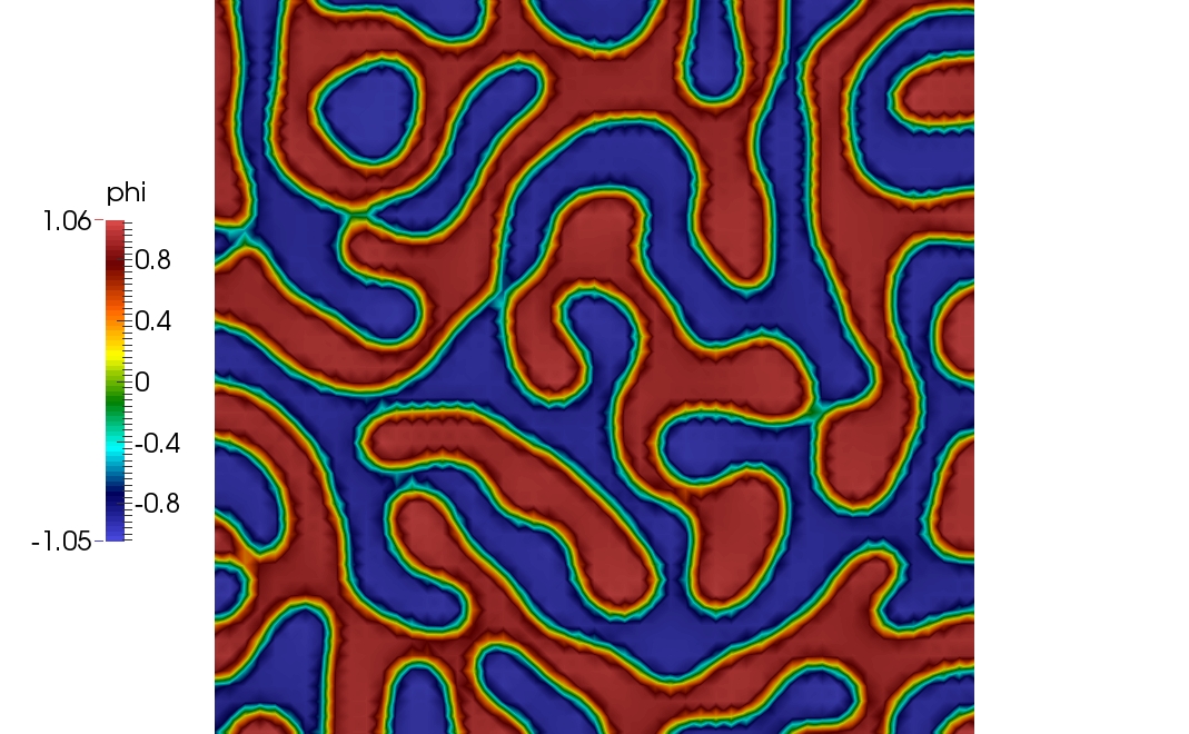
(e) $t=0.5$

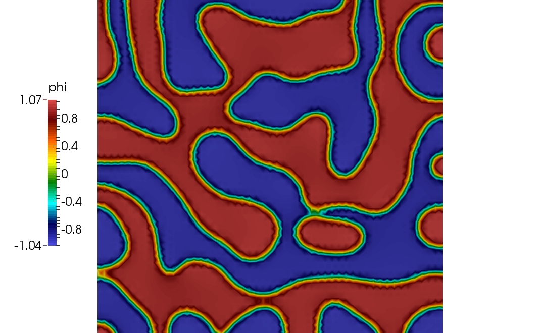
(f) $t=1.$

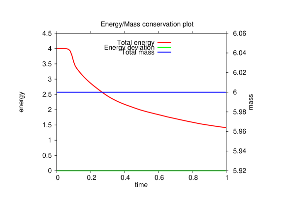
(g) Conservativity/consistency plot

6.7. Test 3 : 2D - parameter values

In this experiment we investigate the effects differing magnitudes of parameter values have on the dynamics of the system. We vary the diffusive terms $m_{r}$ and $m_{j}$.

The initial conditions we consider are given by considering $\Omega=[0,1]^{2}$ and defining subsets

(6.9) $$\Omega_{1}=\{\boldsymbol{x}:\left({\left|x_{1}-1/4\right|^{2}+\left|x_{2}-1/4\right|^{2}}\right)\leq 0.05^{2}\}$$

(6.10) $$\Omega_{2}=\{\boldsymbol{x}:\left({\left|x_{1}-1/4\right|^{2}+\left|x_{2}-3/4\right|^{2}}\right)\leq 0.01^{2}\}$$

(6.11) $$\Omega_{3}=\{\boldsymbol{x}:\left({\left|x_{1}-3/4\right|^{2}+\left|x_{2}-1/4\right|^{2}}\right)\leq 0.01^{2}\}$$

(6.12) $$\Omega_{4}=\{\boldsymbol{x}:\left({\left|x_{1}-3/4\right|^{2}+\left|x_{2}-3/4\right|^{2}}\right)\leq 0.01^{2}\},$$

and choosing

(6.13) $$\phi^{0}=\begin{cases}-1\text{ if }\boldsymbol{x}\in\Omega_{1}\cup\Omega_{2}\cup\Omega_{3}\cup\Omega_{4}\\ 1\text{ otherwise }\end{cases}\qquad\boldsymbol{v}=\boldsymbol{0}.$$

Figure 2 gives some comparitive solution plots at various times in the simulation. Note that by decreasing the magnitude of the dissipative terms, the system takes longer to reach a steady state. The simulation with the smallest values reaches a steady state at $t\approx 32$. Note that when each simulation reaches a steady state $\left\|\boldsymbol{v}_{h}\right\|_{\operatorname{L}_{\infty}(\Omega)}\leq 10^{-5}$ which means that there are no relevant parasitic currents.

Figure 2. 6.7 Test 3 – The solution, $\phi_{h}$ to the quasi-incompressible system with initial conditions (6.13) at various values of $t$. Notice that there are no parasitic currents appearing in the interfacial layer. The velocity tends to zero over the entire domain as time increases.

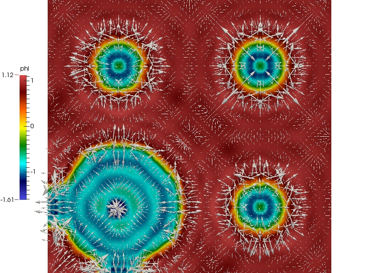
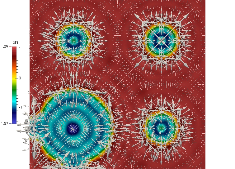
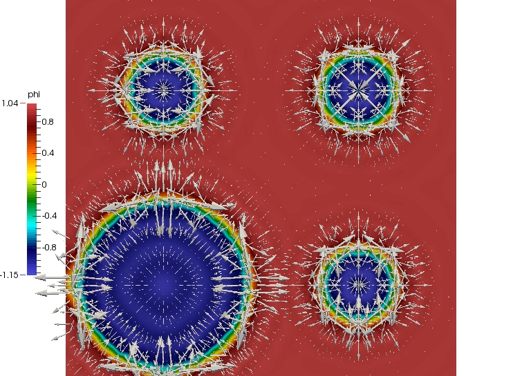
(a) $t=0.1$, left $m_{j}=m_{r}=1$, middle $m_{j}=m_{r}=0.1$, right $m_{j}=m_{r}=0.01$

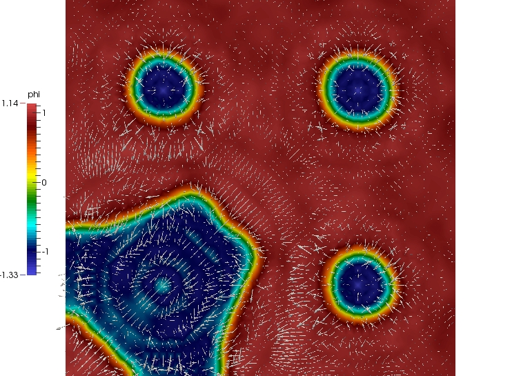
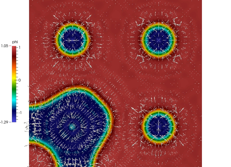
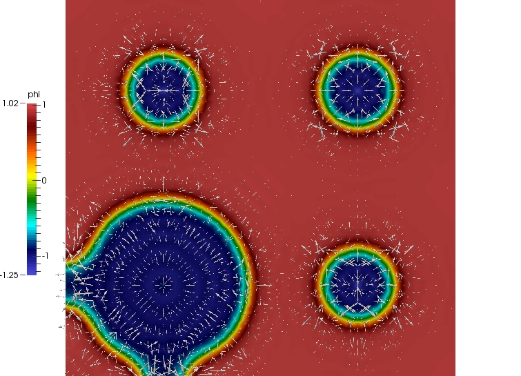
(b) $t=0.25$, left $m_{j}=m_{r}=1$, middle $m_{j}=m_{r}=0.1$, right $m_{j}=m_{r}=0.01$

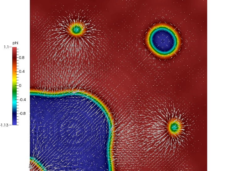
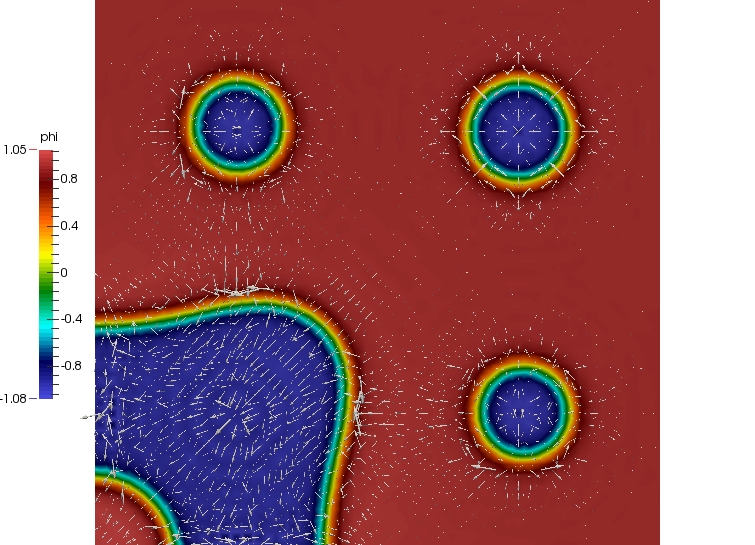
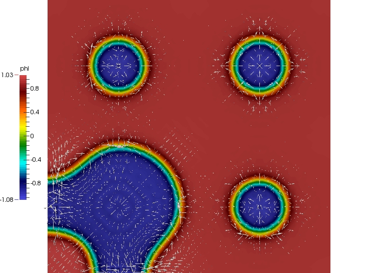
(c) $t=0.5$, left $m_{j}=m_{r}=1$, middle $m_{j}=m_{r}=0.1$, right $m_{j}=m_{r}=0.01$

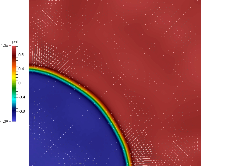
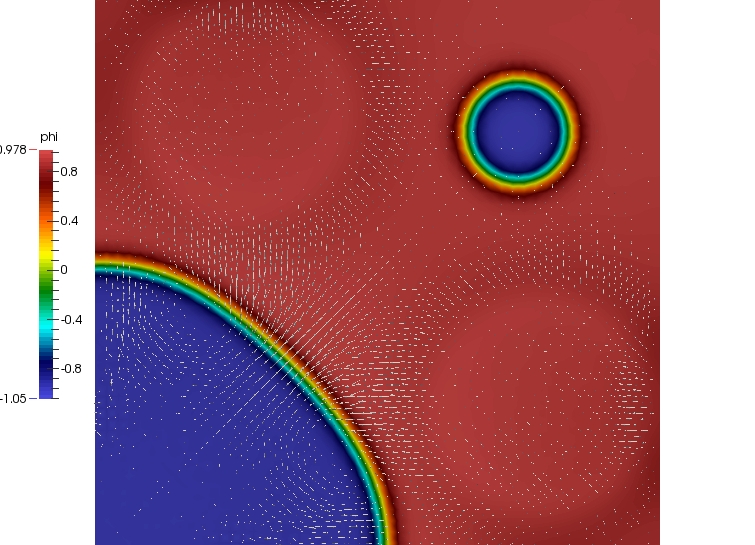
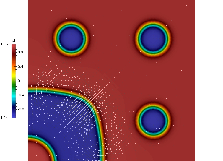
(d) $t=1.4$, left $m_{j}=m_{r}=1$, middle $m_{j}=m_{r}=0.1$, right $m_{j}=m_{r}=0.01$

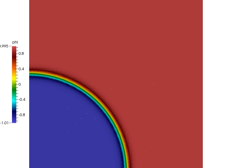
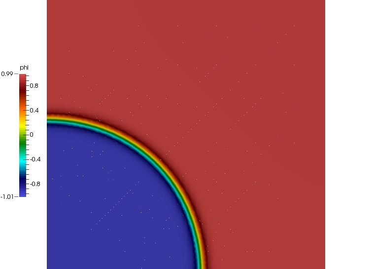
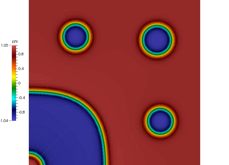
(e) $t=5$, left $m_{j}=m_{r}=1$, middle $m_{j}=m_{r}=0.1$, right $m_{j}=m_{r}=0.01$

6.8. Test 4 : 2D rotating coordinate system

Due to the invariance properties of the model (2.9) including the full Navier-Stokes tensor should we desire computations in a rotating coordinate system the required changes are very simple. We need only account for inertial or fictitious forces. This is in contrast to the model described in [AGG12] which does not behave well with respect to coordinate changes involving rotating coordinate systems. The fictitious forces we need to introduce are the Coriolis and the centrifugal force. In case we consider a planar model problem where the system rotates with angular velocity $\omega$ around an axis which is perpendicular to the computational domain then the modified sytem of equations reads

(6.14) $$\begin{split}\partial_{t}{\phi}+\operatorname{div}\left({\phi\boldsymbol{v}}\right)&=c_{+}\left({m_{j}\Delta-m_{r}}\right)\left({c_{+}\mu(\phi)+c_{-}\lambda}\right)\\ \rho(\phi)\left({\partial_{t}{\boldsymbol{v}}+\left({{\boldsymbol{v}}^{{\boldsymbol{\intercal}}}\nabla}\right)\boldsymbol{v}}\right)+\nabla\left({p(\phi)+\lambda}\right)&=\operatorname{div}(\boldsymbol{\sigma}_{NS})+\gamma\phi\nabla\Delta\phi-\rho(\phi){\boldsymbol{\Omega}}\times({\boldsymbol{\Omega}}\times{\boldsymbol{x}})\\ &\qquad-2\rho(\phi)\boldsymbol{\Omega}\times\boldsymbol{v}\\ \operatorname{div}{\boldsymbol{v}}&=c_{-}\left({m_{j}\Delta-m_{r}}\right)\left({c_{+}\mu(\phi)+c_{-}\lambda}\right)\end{split}$$

where $\boldsymbol{\Omega}={(0,0,\omega)}^{{\boldsymbol{\intercal}}}$ and we embed $\boldsymbol{v}$ to $\mathbb{R}^{3}$ as $(\boldsymbol{v};0)$ for the sake of the vector product.

We now use the original system including the Navier Stokes tensor (2.9) and energy consistent approximations for this problem follow our arguments given a standard (signed) discretisation of the Navier–Stokes tensor. Indeed, the discretisation is identical to (5.1) with the exception of equation (5.1)₂ which now reads

(6.15) $$\begin{split}0&=\int_{\Omega}\rho(\phi_{h}^{n+\tfrac{1}{2}})\frac{\boldsymbol{v}_{h}^{n+1}-\boldsymbol{v}_{h}^{n}}{k_{n}}\cdot\boldsymbol{\Xi}+\rho(\phi_{h}^{n+\tfrac{1}{2}})\left({\left({\boldsymbol{v}_{h}^{n+\tfrac{1}{2}}\cdot\nabla}\right)\boldsymbol{v}_{h}^{n+\tfrac{1}{2}}}\right)\cdot\boldsymbol{\Xi}\\ &\qquad\qquad-\frac{1}{2}\rho(\phi_{h}^{n+\tfrac{1}{2}})\nabla\left({\left|\boldsymbol{v}_{h}^{n+\tfrac{1}{2}}\right|^{2}}\right)\cdot\boldsymbol{\Xi}-\eta\mathscr{A}_{2}\left({{\boldsymbol{v}_{h}^{n+\tfrac{1}{2}}},{\boldsymbol{\Xi}}}\right)+\nabla b_{h}^{n+\tfrac{1}{2}}\cdot\boldsymbol{\Xi}\\ &\qquad\qquad+\frac{\phi_{h}^{n+\tfrac{1}{2}}}{c_{+}}\nabla(a_{h}^{n+\tfrac{1}{2}}-c_{-}b_{h}^{n+\tfrac{1}{2}})\cdot\boldsymbol{\Xi}+\left({\rho(\phi_{h}^{n+\tfrac{1}{2}})\boldsymbol{\Omega}\times\left({\boldsymbol{\Omega}\times\boldsymbol{x}}\right)}\right){\cdot\boldsymbol{\Xi}}\\ &\qquad\qquad+\left({2\rho(\phi_{h}^{n+\tfrac{1}{2}})\boldsymbol{\Omega}\times\boldsymbol{v}_{h}^{n+\tfrac{1}{2}}}\right){\cdot\boldsymbol{\Xi}}\\ &\qquad+\int_{\mathscr{E}}\left({{-}\mathrel{\ooalign{\cr\kern 1.0pt$\{$\cr\kern-0.5pt$\{$}}\boldsymbol{\Xi}\mathrel{\ooalign{$\}$\cr\kern-1.5pt$\}$\cr\kern-1.0pt}}\otimes\mathrel{\ooalign{\cr\kern 1.0pt$\{$\cr\kern-0.5pt$\{$}}\rho(\phi_{h}^{n+\tfrac{1}{2}})\boldsymbol{v}_{h}^{n+\tfrac{1}{2}}\mathrel{\ooalign{$\}$\cr\kern-1.5pt$\}$\cr\kern-1.0pt}}}\right):\left\llbracket\boldsymbol{v}_{h}^{n+\tfrac{1}{2}}\right\rrbracket_{\otimes}\\ &\qquad\qquad{+}\frac{1}{2}\left\llbracket\left|\boldsymbol{v}_{h}^{n+\tfrac{1}{2}}\right|^{2}\right\rrbracket\cdot\mathrel{\ooalign{\cr\kern 1.0pt$\{$\cr\kern-0.5pt$\{$}}\rho(\phi_{h}^{n+\tfrac{1}{2}})\boldsymbol{\Xi}\mathrel{\ooalign{$\}$\cr\kern-1.5pt$\}$\cr\kern-1.0pt}}\\ &\qquad\qquad-\left\llbracket b_{h}^{n+\tfrac{1}{2}}\right\rrbracket\cdot\mathrel{\ooalign{\cr\kern 1.0pt$\{$\cr\kern-0.5pt$\{$}}\boldsymbol{\Xi}\mathrel{\ooalign{$\}$\cr\kern-1.5pt$\}$\cr\kern-1.0pt}}-\frac{1}{c_{+}}\left\llbracket a_{h}^{n+\tfrac{1}{2}}-c_{-}b_{h}^{n+\tfrac{1}{2}}\right\rrbracket\cdot\mathrel{\ooalign{\cr\kern 1.0pt$\{$\cr\kern-0.5pt$\{$}}\phi_{h}^{n+\tfrac{1}{2}}\boldsymbol{\Xi}\mathrel{\ooalign{$\}$\cr\kern-1.5pt$\}$\cr\kern-1.0pt}},\end{split}$$

where

(6.16) $$\begin{split}\mathscr{A}_{2}\left({\boldsymbol{v}_{h},\boldsymbol{\Xi}}\right)&=-\int_{\Omega}\left({\eta_{1}-\frac{2}{d}\eta_{2}}\right){\left({\operatorname{div}\left({\boldsymbol{v}_{h}}\right)\boldsymbol{I}_{d}}\right)}{:}{\mathrm{D}\boldsymbol{\Xi}}+\eta_{2}{\left({\mathrm{D}\boldsymbol{v}_{h}+{\mathrm{D}\boldsymbol{v}}^{{\boldsymbol{\intercal}}}}\right)}{:}{\mathrm{D}\boldsymbol{\Xi}}\\ &\qquad+\left({\eta_{1}-\frac{2}{d}\eta_{2}}\right)\int_{\mathscr{E}\cup\partial\Omega}{\left({\left\llbracket\boldsymbol{v}_{h}\right\rrbracket\boldsymbol{I}_{d}}\right)}{:}{\mathrel{\ooalign{\cr\kern 1.0pt$\{$\cr\kern-0.5pt$\{$}}\mathrm{D}\boldsymbol{\Xi}\mathrel{\ooalign{$\}$\cr\kern-1.5pt$\}$\cr\kern-1.0pt}}}+{\left({\mathrel{\ooalign{\cr\kern 1.0pt$\{$\cr\kern-0.5pt$\{$}}\operatorname{div}\left({\boldsymbol{v}_{h}}\right)\mathrel{\ooalign{$\}$\cr\kern-1.5pt$\}$\cr\kern-1.0pt}}\boldsymbol{I}_{d}}\right)}{:}{\left\llbracket\boldsymbol{\Xi}\right\rrbracket_{\otimes}}\\ &\qquad+\eta_{2}\int_{\mathscr{E}\cup\partial\Omega}{\left({\left\llbracket\boldsymbol{v}_{h}\right\rrbracket_{\otimes}+{\left\llbracket\boldsymbol{v}_{h}\right\rrbracket_{\otimes}}^{{\boldsymbol{\intercal}}}}\right)}{:}{\mathrel{\ooalign{\cr\kern 1.0pt$\{$\cr\kern-0.5pt$\{$}}\mathrm{D}\boldsymbol{\Xi}\mathrel{\ooalign{$\}$\cr\kern-1.5pt$\}$\cr\kern-1.0pt}}}+{\left\llbracket\boldsymbol{\Xi}\right\rrbracket_{\otimes}}{:}{\mathrel{\ooalign{\cr\kern 1.0pt$\{$\cr\kern-0.5pt$\{$}}\left({\mathrm{D}\boldsymbol{v}_{h}+{\left({\mathrm{D}\boldsymbol{v}_{h}}\right)}^{{\boldsymbol{\intercal}}}}\right)\mathrel{\ooalign{$\}$\cr\kern-1.5pt$\}$\cr\kern-1.0pt}}}\\ &\qquad-\int_{\mathscr{E}}\frac{\sigma}{h}{\left\llbracket\boldsymbol{v}_{h}\right\rrbracket_{\otimes}}{:}{\left\llbracket\boldsymbol{\Xi}\right\rrbracket_{\otimes}},\end{split}$$

represents an interior penalty type discretisation of the Navier–Stokes tensor which is signed when the penalty parameter $\sigma$ is chosen large enough.

We also have access to a Lyapanov functional representing the energy of the system. In this case

(6.17) $$\begin{split}\,\mathrm{d}_{t}\bigg{(}\int_{\Omega}W(\phi)&+\frac{\rho(\phi)}{2}\left|\boldsymbol{v}\right|^{2}+\frac{\gamma}{2}\left|\nabla\phi\right|^{2}-\omega^{2}\frac{\rho(\phi)}{2}\left|\boldsymbol{x}\right|^{2}\bigg{)}\\ &=-\int_{\Omega}m_{j}\left|\nabla\left({c_{+}\mu(\phi)+c_{-}\lambda}\right)\right|^{2}+m_{r}\left({c_{+}\mu(\phi)+c_{-}\lambda}\right)^{2}+{\mathrm{D}\boldsymbol{v}}{:}{\boldsymbol{\sigma}_{NS}}.\end{split}$$

Using the arguments presented above it can be shown that the fully discrete scheme (5.1) with (5.1)₂ replaced by (6.15) satisfies both mass conservation as well as the following energy dissipation equality

(6.18) $$\begin{split}\int_{\Omega}W(\phi_{h}^{n+1})&+\frac{1}{2}\rho(\phi_{h}^{n+1})\left|\boldsymbol{v}_{h}^{n+1}\right|^{2}+\frac{\gamma}{2}\left|\boldsymbol{q}_{h}^{n+1}\right|^{2}-\omega^{2}\frac{\rho(\phi_{h}^{n+1})}{2}\left|\boldsymbol{x}\right|^{2}\\ &=\int_{\Omega}W(\phi_{h}^{n})+\frac{1}{2}\rho(\phi_{h}^{n})\left|\boldsymbol{v}_{h}^{n}\right|^{2}+\frac{\gamma}{2}\left|\boldsymbol{q}_{h}^{n}\right|^{2}-\omega^{2}\frac{\rho(\phi_{h}^{n})}{2}\left|\boldsymbol{x}\right|^{2}\\ &\qquad-k_{n}\Bigg{(}\int_{\Omega}m_{r}\left({a_{h}^{n+\tfrac{1}{2}}}\right)^{2}-m_{j}\mathscr{A}_{1}\left({a_{h}^{n+\tfrac{1}{2}},a_{h}^{n+\tfrac{1}{2}}}\right)\\ &\qquad\qquad-\mathscr{A}_{2}\left({\boldsymbol{v}_{h}^{n+\tfrac{1}{2}},\boldsymbol{v}_{h}^{n+\tfrac{1}{2}}}\right)\Bigg{)},\end{split}$$

with $\mathscr{A}_{2}$ given by (6.16).

In Figure 3 we illustrate a numerical simulation using these principles. We take $\Omega$ to be a polyhedral approximation to the unit circle. We set $\eta_{1}=0.001$ and $\eta_{2}=0.005$. We use an initial condition which is a offset bubble from the coordinate axis, i.e.,

(6.19) $$\phi^{0}:=\begin{cases}-1\text{ if }\left({\left|x_{1}+0.1\right|^{2}+\left|x_{2}+0.1\right|^{2}}\right)\leq 0.1^{2}\\ 1\text{ otherwise}\end{cases},\qquad\boldsymbol{v}^{0}=\boldsymbol{0}.$$

We show some solution plots at various times as well as the mass/energy plot.

Figure 3. 6.8 Test 4 – The solution, $\phi_{h}$ to the quasi-incompressible system with initial conditions (6.19) at various values of $t$.

(a) $t=0.01$

(b) $t=1.75$

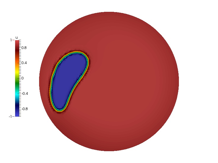
(c) $t=2.61$

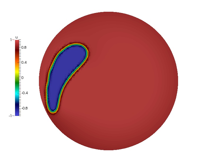
(d) $t=2.91$

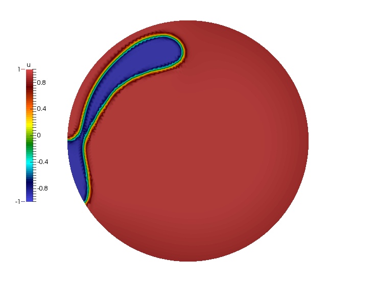
(e) $t=4$

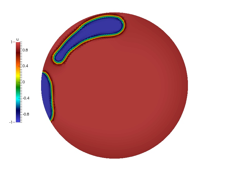
(f) $t=4.5$

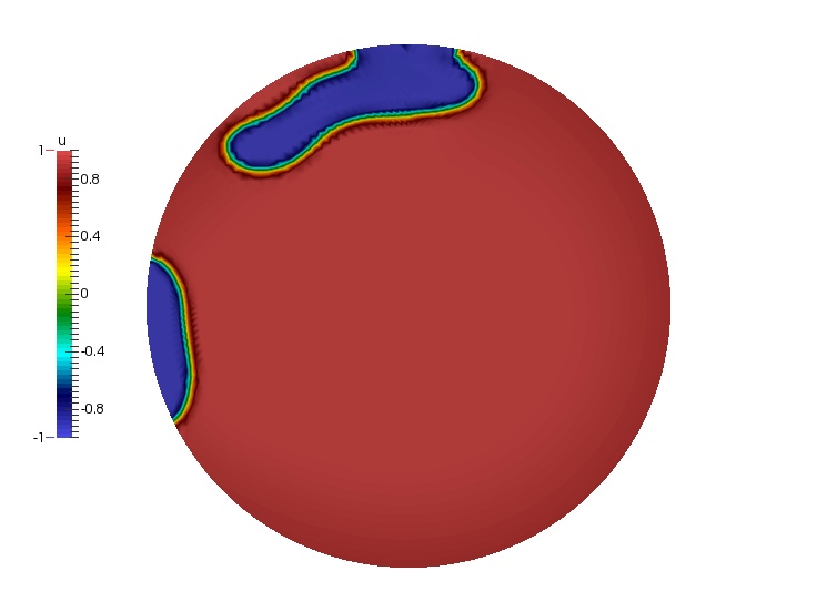
(g) $t=4.98$

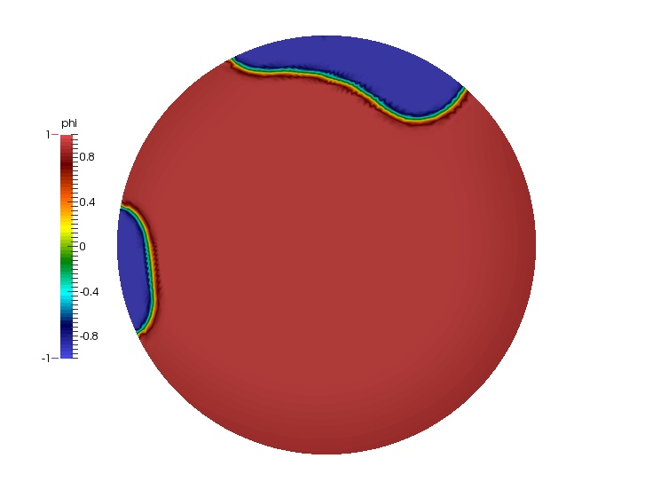
(h) $t=6.52$

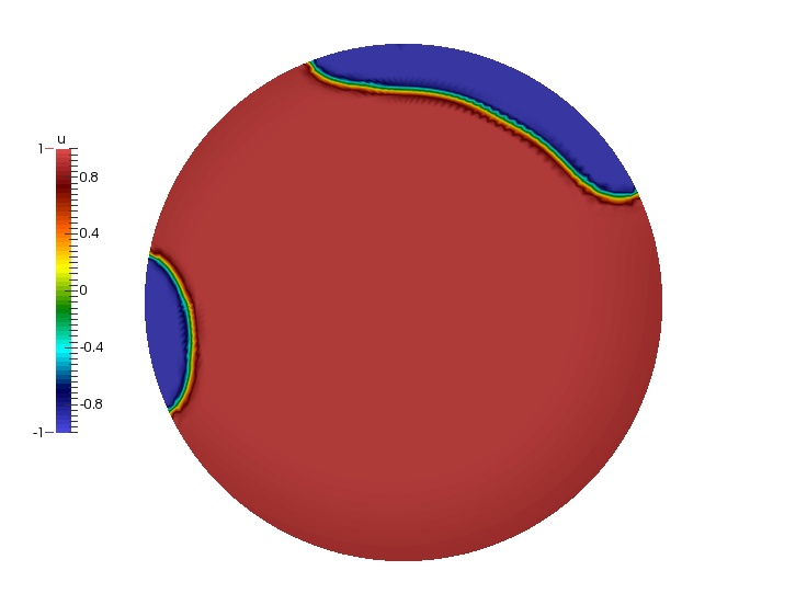
(i) $t=7.64$

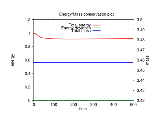
(j) Conservativity/consistency plot

6.9. Test 5 : 2D - Rayleigh Taylor instability

In this test we examine the robustness of the scheme when a denser fluid lies on top of a lighter one. In this case it is expected that waves will form over the interface which can give rise to the formation of plumes.

We take $\Omega=[-1,1]\times[-2,2]$ and choose

(6.20) $$\phi^{0}:=\begin{cases}1\text{ if }x_{2}\leq 0\\ -1\text{ otherwise}\end{cases},\qquad\boldsymbol{v}^{0}=\bigg{(}\begin{array}[]{c}0\\ {\left({1+\operatorname{cos}\left({\pi x_{1}}\right)}\right)\left({1+\operatorname{cos}\left({{\pi x_{2}}/{2}}\right)}\right)}/{4}\end{array}\bigg{)}.$$

We also modify (5.1)₂ to take gravitational effects into account. In this case (5.1)₂ takes the form

(6.21) $$\begin{split}0&=\int_{\Omega}\rho(\phi_{h}^{n+\tfrac{1}{2}})\frac{\boldsymbol{v}_{h}^{n+1}-\boldsymbol{v}_{h}^{n}}{k_{n}}\cdot\boldsymbol{\Xi}+\rho(\phi_{h}^{n+\tfrac{1}{2}})\left({\left({\boldsymbol{v}_{h}^{n+\tfrac{1}{2}}\cdot\nabla}\right)\boldsymbol{v}_{h}^{n+\tfrac{1}{2}}}\right)\cdot\boldsymbol{\Xi}\\ &\qquad\qquad-\frac{1}{2}\rho(\phi_{h}^{n+\tfrac{1}{2}})\nabla\left({\left|\boldsymbol{v}_{h}^{n+\tfrac{1}{2}}\right|^{2}}\right)\cdot\boldsymbol{\Xi}-\eta\mathscr{A}_{2}\left({{\boldsymbol{v}_{h}^{n+\tfrac{1}{2}}},{\boldsymbol{\Xi}}}\right)+\nabla b_{h}^{n+\tfrac{1}{2}}\cdot\boldsymbol{\Xi}\\ &\qquad\qquad+\frac{\phi_{h}^{n+\tfrac{1}{2}}}{c_{+}}\nabla(a_{h}^{n+\tfrac{1}{2}}-c_{-}b_{h}^{n+\tfrac{1}{2}})\cdot\boldsymbol{\Xi}+\rho(\phi^{n+\tfrac{1}{2}})\boldsymbol{g}\cdot\boldsymbol{\Xi}\\ &\qquad+\int_{\mathscr{E}}\left({{-}\mathrel{\ooalign{\cr\kern 1.0pt$\{$\cr\kern-0.5pt$\{$}}\boldsymbol{\Xi}\mathrel{\ooalign{$\}$\cr\kern-1.5pt$\}$\cr\kern-1.0pt}}\otimes\mathrel{\ooalign{\cr\kern 1.0pt$\{$\cr\kern-0.5pt$\{$}}\rho(\phi_{h}^{n+\tfrac{1}{2}})\boldsymbol{v}_{h}^{n+\tfrac{1}{2}}\mathrel{\ooalign{$\}$\cr\kern-1.5pt$\}$\cr\kern-1.0pt}}}\right):\left\llbracket\boldsymbol{v}_{h}^{n+\tfrac{1}{2}}\right\rrbracket_{\otimes}\\ &\qquad\qquad{+}\frac{1}{2}\left\llbracket\left|\boldsymbol{v}_{h}^{n+\tfrac{1}{2}}\right|^{2}\right\rrbracket\cdot\mathrel{\ooalign{\cr\kern 1.0pt$\{$\cr\kern-0.5pt$\{$}}\rho(\phi_{h}^{n+\tfrac{1}{2}})\boldsymbol{\Xi}\mathrel{\ooalign{$\}$\cr\kern-1.5pt$\}$\cr\kern-1.0pt}}\\ &\qquad\qquad-\left\llbracket b_{h}^{n+\tfrac{1}{2}}\right\rrbracket\cdot\mathrel{\ooalign{\cr\kern 1.0pt$\{$\cr\kern-0.5pt$\{$}}\boldsymbol{\Xi}\mathrel{\ooalign{$\}$\cr\kern-1.5pt$\}$\cr\kern-1.0pt}}-\frac{1}{c_{+}}\left\llbracket a_{h}^{n+\tfrac{1}{2}}-c_{-}b_{h}^{n+\tfrac{1}{2}}\right\rrbracket\cdot\mathrel{\ooalign{\cr\kern 1.0pt$\{$\cr\kern-0.5pt$\{$}}\phi_{h}^{n+\tfrac{1}{2}}\boldsymbol{\Xi}\mathrel{\ooalign{$\}$\cr\kern-1.5pt$\}$\cr\kern-1.0pt}},\end{split}$$

where $\boldsymbol{g}={\left({0,0.01}\right)}^{{\boldsymbol{\intercal}}}$ is a gravitational constant. In Figure 4 we show results from a numerical experiment with the initial conditions given in (6.20).

Figure 4. 6.9 Test 5 – The solution, $\phi_{h}$ to the quasi-incompressible system with initial conditions (6.20) at various values of $t$.

(a) $t=0.01$

(b) $t=3$

(c) $t=5$

(d) $t=6.65$

(e) $t=8.1$

(f) $t=9.11$

(g) $t=9.54$

(h) $t=13$

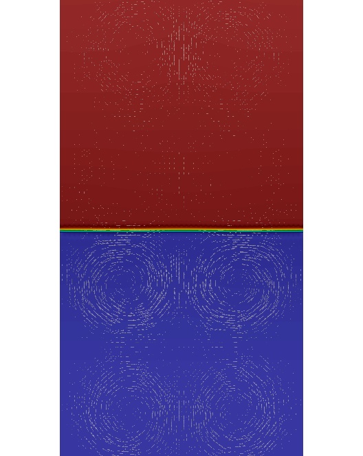
(i) $t=39.95$

6.10 Remark (guaranteeing positivity of $\rho(\phi)$ and solvability of the numerical scheme).

The energy dissipation equality of the numerical scheme given in Theorem 5.2 gives us no information on the solvability of the discrete scheme. In addition, the positivity of the density $\rho(\phi)$ is not guaranteed. Numerically, for low denisty ratios, like those in tests 1–5 where $\rho_{2}/\rho_{1}=2$, positivity and solvability is observed. However, for higher density ratios, this is no longer the case. To overcome this difficulty, there are at least three possibilities:

The first is to use a different energy density, which penalises values of $\phi$ outside the interval $[-1,1]$. To that end, we introduce

(6.22) $$W(\phi)=(1+\phi)^{2}(1-\phi)^{2}+A\left({\left({\phi-1+\left|\phi-1\right|}\right)^{2}+\left({-\phi-1+\left|-\phi-1\right|}\right)^{2}}\right),$$

where $A$ is a large parameter chosen relative to the density ratio $\rho_{2}/\rho_{1}$ to ensure the density is positive. From a modelling point of view, the energy density $W$ is purely artificial and thus can be chosen reasonably freely.

The second approach is to use a cutoff of the density function as detailed in [Grü]. The main idea is to use the densities of the pure phases when $\phi\not\in[-1,1]$.

The third approach is to modify the mobilities such that they are functions of $\phi$ that are degenerate when $\phi\not\in[-1,1]$ in a similar light to [GR00].

The first approach fits into the analytical framework developed in this contribution, the second and third do not. As such, we will not persue the case of denisty cutoff functions or nonconstant mobilities further but we believe that our results are extendable to these cases.

6.11. Test 6 : 1D - High density ratios

In this test we examine the numerical schemes behaviour for various density ratios based on the modified energy density (6.22). In Figures 5–8 we study a 1D equivalent problem to that given in Test 2 for various density ratios ranging from $\rho_{2}/\rho_{1}=2$ to $\rho_{2}/\rho_{1}=1000$. We note that with $A=\left({\rho_{2}/\rho_{1}}\right)^{2}$ the density $\rho(\phi)>0$ and as the density ratio increases the simulation takes longer to achieve a steady state.

Figure 5. 6.11 Test 6 – The solution, $\phi_{h}$ to the quasi-incompressible system, using the modified double well in (6.22) with $A=(\rho_{1}/\rho_{2})^{2}$, with initial conditions (6.7) at various values of $t$. In this case $\rho_{2}/\rho_{1}=2$ and $\max{\phi}=1.2175$ hence $\rho(\phi)>0$ for all time.

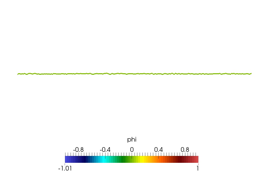
(a) $t=0$

(b) $t=0.09$

(c) $t=0.43$

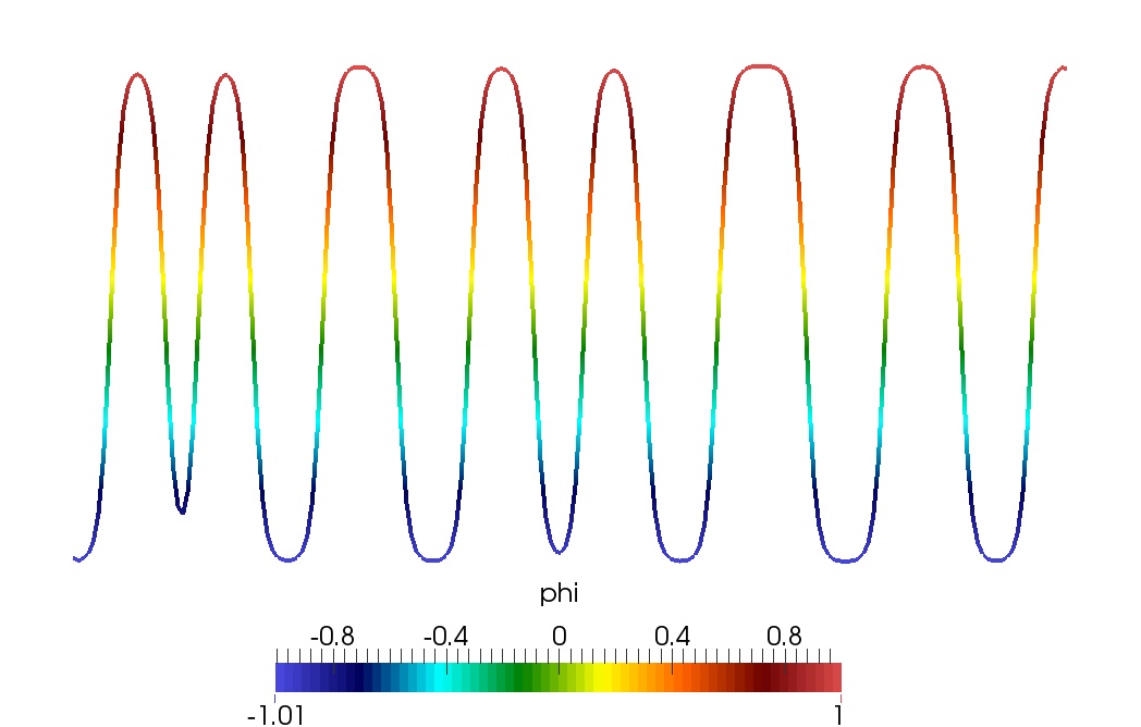
(d) $t=5$

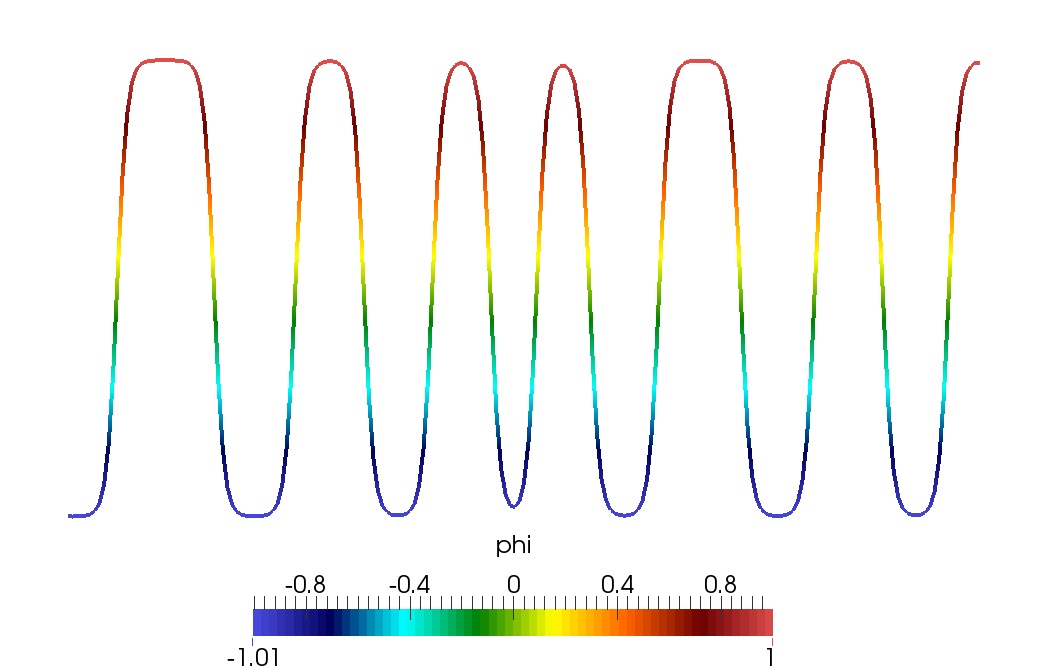
(e) $t=10$

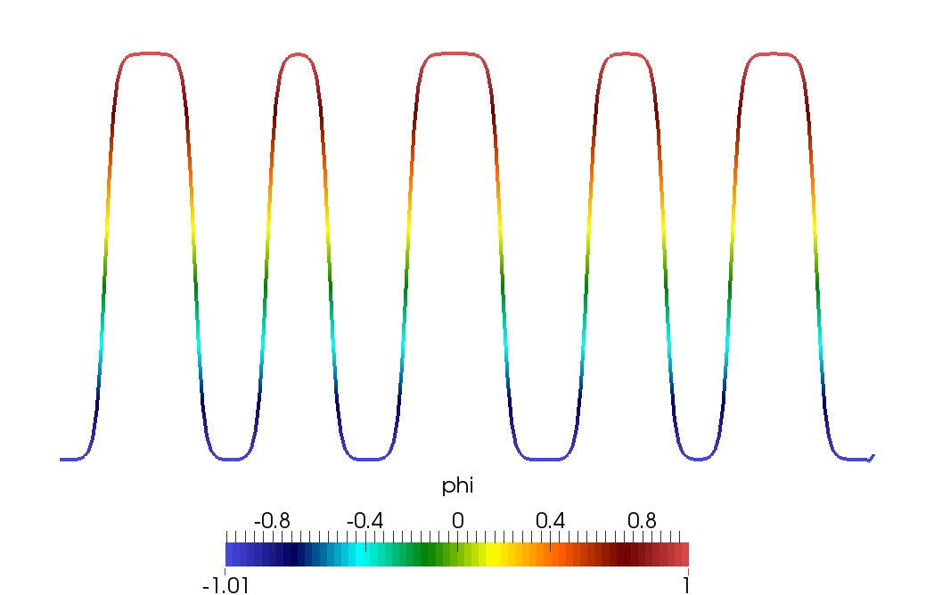
(f) $t=100$

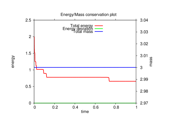
(g) Conservativity/consistency plot

Figure 6. 6.11 Test 6 – As Figure 5 but in this case $\rho_{2}/\rho_{1}=10$ and $\max{\phi}=1.0233$ hence $\rho(\phi)>0$ for all time.

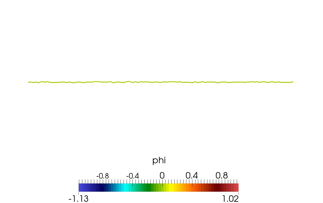
(a) $t=0$

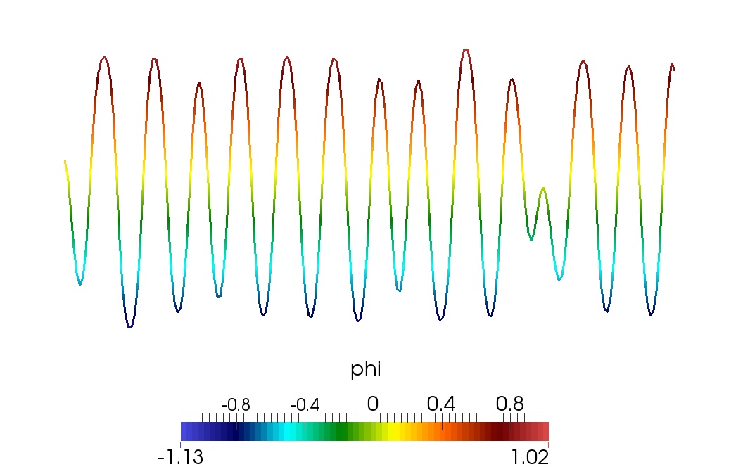
(b) $t=0.43$

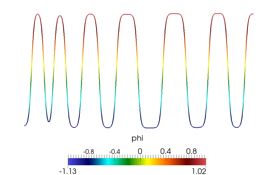
(c) $t=10$

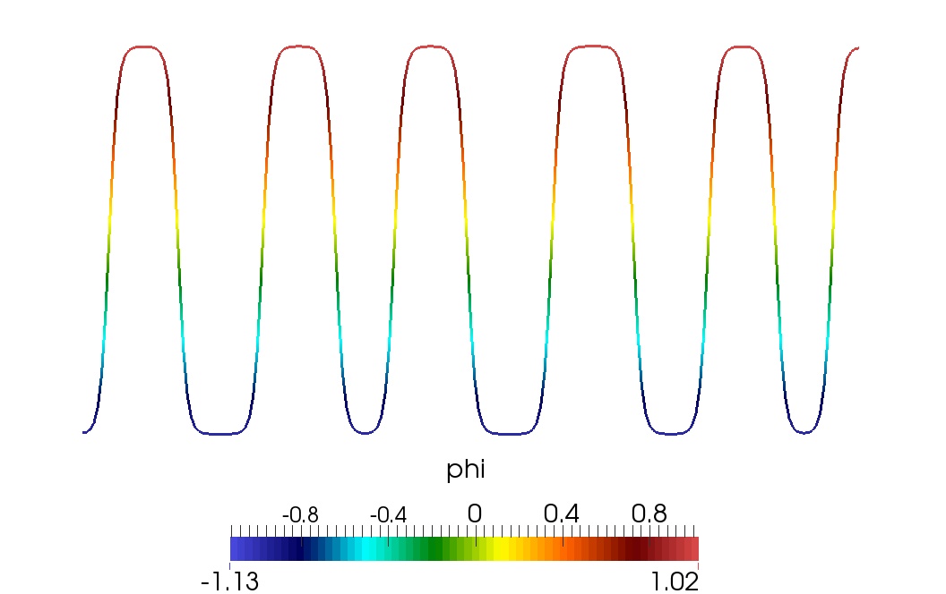
(d) $t=100$

Figure 7. 6.11 Test 6 – As Figure 5 but in this case $\rho_{2}/\rho_{1}=100$ and $\max{\phi}=1.0052$ hence $\rho(\phi)>0$ for all time.

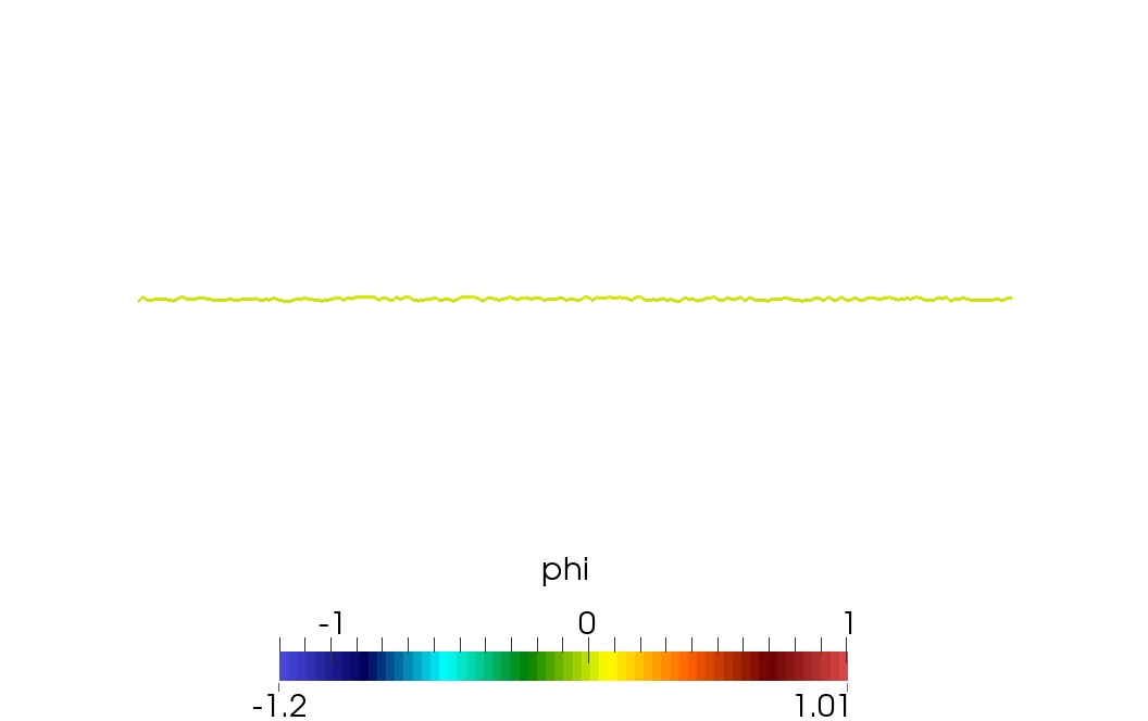
(a) $t=0$

(b) $t=0.43$

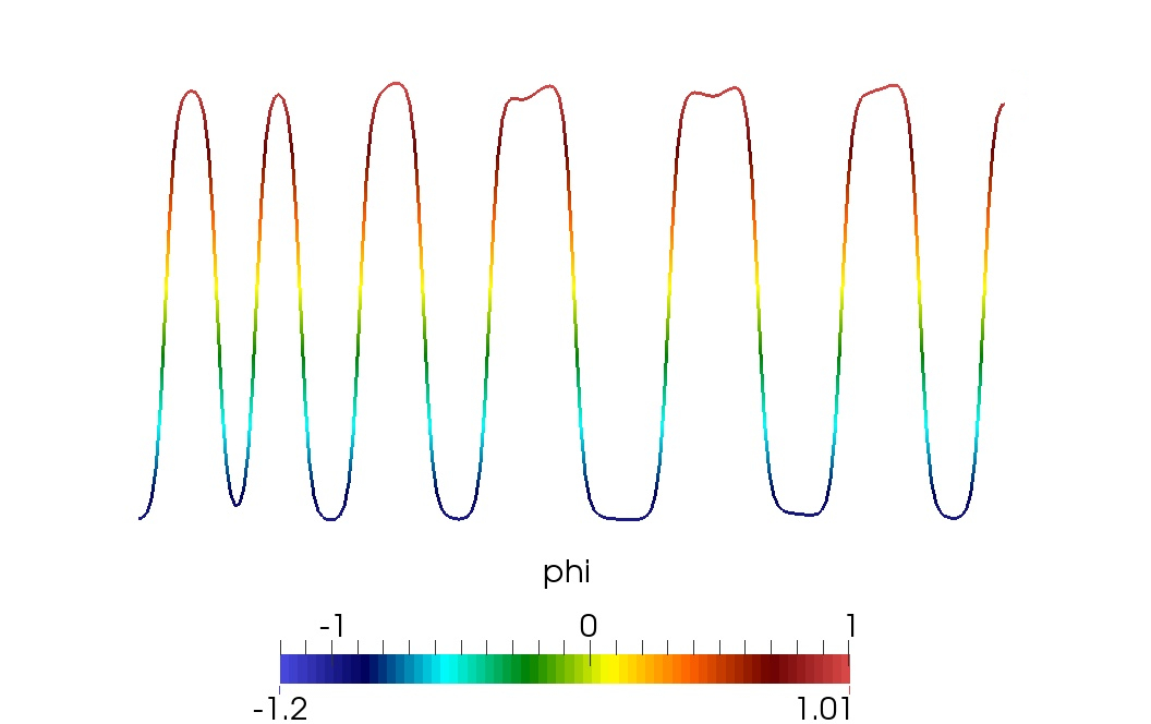
(c) $t=10$

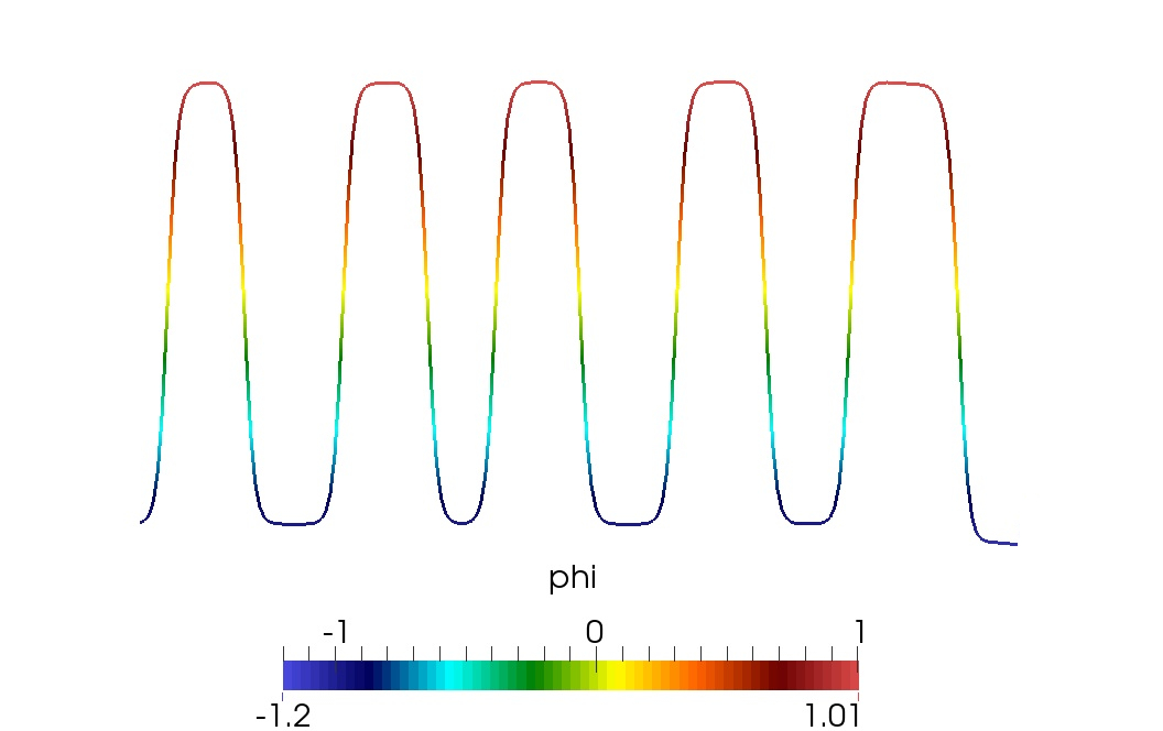
(d) $t=100$

Figure 8. 6.11 Test 6 – As Figure 5 but in this case $\rho_{2}/\rho_{1}=1000$ and $\max{\phi}=1.0006$ hence $\rho(\phi)>0$ for all time.

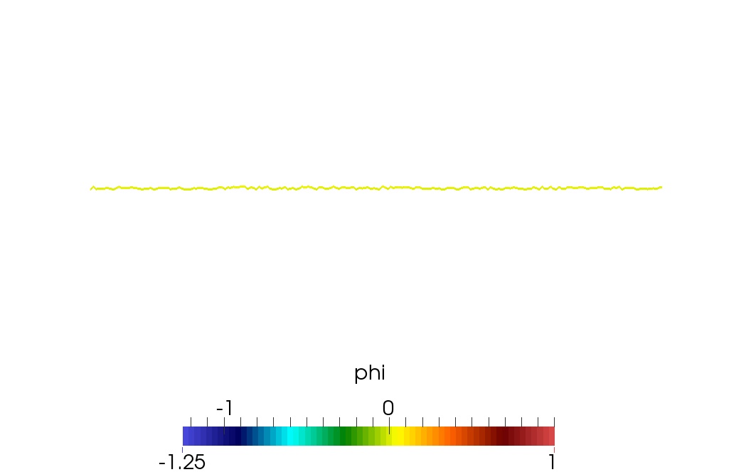
(a) $t=0$

(b) $t=0.43$

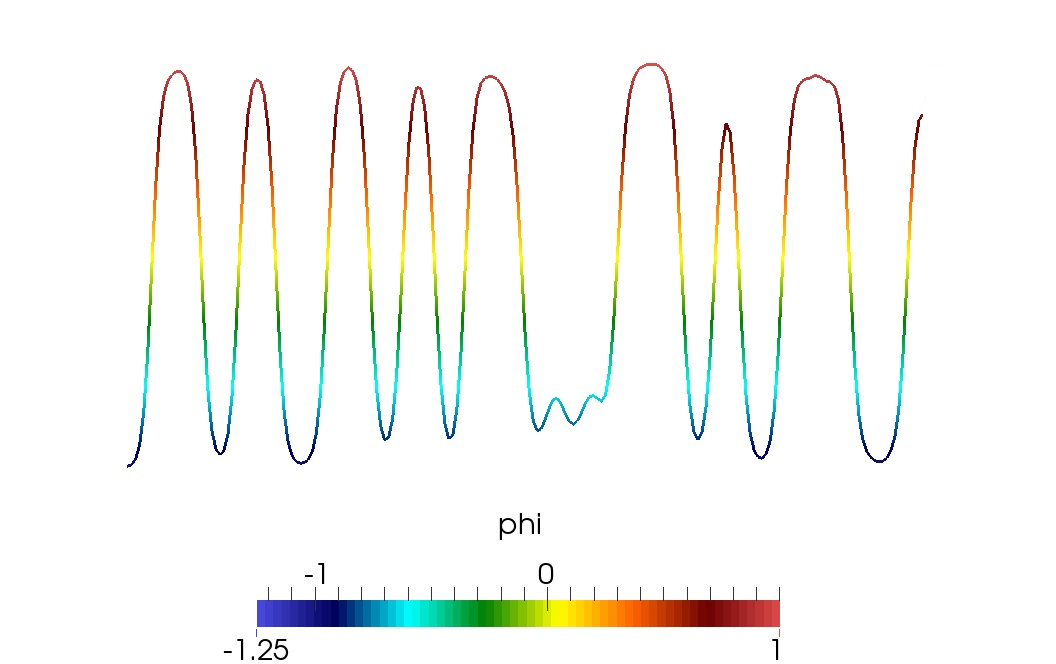
(c) $t=10$

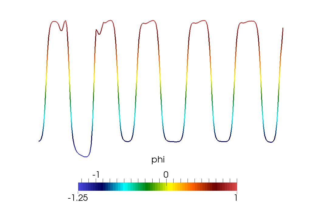
(d) $t=100$