Safe Screening with Variational Inequalities and Its Application to Lasso

Abstract

Sparse learning techniques have been routinely used for feature selection as the resulting model usually has a small number of non-zero entries. Safe screening, which eliminates the features that are guaranteed to have zero coefficients for a certain value of the regularization parameter, is a technique for improving the computational efficiency. Safe screening is gaining increasing attention since 1) solving sparse learning formulations usually has a high computational cost especially when the number of features is large and 2) one needs to try several regularization parameters to select a suitable model. In this paper, we propose an approach called “Sasvi” (Safe screening with variational inequalities). Sasvi makes use of the variational inequality that provides the sufficient and necessary optimality condition for the dual problem. Several existing approaches for Lasso screening can be casted as relaxed versions of the proposed Sasvi, thus Sasvi provides a stronger safe screening rule. We further study the monotone properties of Sasvi for Lasso, based on which a sure removal regularization parameter can be identified for each feature. Experimental results on both synthetic and real data sets are reported to demonstrate the effectiveness of the proposed Sasvi for Lasso screening.

1 Introduction

Sparse learning [2, 12] is an effective technique for analyzing high dimensional data. It has been applied successfully in various areas, such as machine learning, signal processing, image processing, medical imaging, and so on. In general, the $\ell_{1}$-regularized sparse learning can be formulated as:

$$\min_{\bm{\beta}}\quad\mbox{loss}(\bm{\beta})+\lambda\|\bm{\beta}\|_{1},$$ (1)

where $\bm{\beta}\in\mathbb{R}^{p}$ contains the model coefficients, $\mbox{loss}(\bm{\beta})$ is a loss function defined on the design matrix $X\in\mathbb{R}^{n\times p}$ and the response $\mathbf{y}\in\mathbb{R}^{n}$, and $\lambda$ is a positive regularization parameter that balances the tradeoff between the loss function and the $\ell_{1}$ regularization. Let $\mathbf{x}^{i}\in\mathbb{R}^{p}$ denote the $i$-th sample that corresponds to the transpose of the $i$-th row of $X$, and let $\mathbf{x}_{j}\in\mathbb{R}^{n}$ denote the $j$-th feature that corresponds to the $j$-th column of $X$. We use $\mbox{loss}(\bm{\beta})=\frac{1}{2}\|X\bm{\beta}-\mathbf{y}\|_{2}^{2}=\frac{1}{2}\sum_{i=1}^{n}(y_{i}-\bm{\beta}^{T}\mathbf{x}^{i})^{2}$ in Lasso [12] and $\mbox{loss}(\bm{\beta})=\sum_{i=1}^{n}\log(1+\exp(-y_{i}\bm{\beta}^{T}\mathbf{x}^{i}))$ in sparse logistic regression [6].

Since the optimal $\lambda$ is usually unknown in practical applications, we need to solve formulation (1) corresponding to a series of regularization parameter $\lambda_{1}>\lambda_{2}>\ldots>\lambda_{k}$, obtain the solutions $\bm{\beta}^{*}_{1},\bm{\beta}^{*}_{2},\ldots,\bm{\beta}^{*}_{k}$, and then select the solution that is optimal in terms of a pre-specified criterion, e.g., Schwarz Bayesian information criterion [11] and cross-validation. The well-known LARS approach [3] can be modified to obtain the full piecewise linear Lasso solution path. Other approaches such as interior point [6], coordinate descent [4] and accelerated gradient descent [8] usually solve formulation (1) corresponding to a series of pre-defined parameters.

The solutions $\bm{\beta}^{*}_{k},k=1,2,\ldots,$ are sparse in that many of their coefficients are zero. Taking advantage of the nature of sparsity, the screening techniques have been proposed for accelerating the computation. Specifically, given a solution $\bm{\beta}^{*}_{1}$ at the regularization parameter $\lambda_{1}$, if we can identify the features that are guaranteed to have zero coefficients in $\bm{\beta}^{*}_{2}$ at the regularization parameter $\lambda_{2}$, then the cost for computing $\bm{\beta}^{*}_{2}$ can be saved by excluding those inactive features. There are two categories of screening techniques: 1) the safe screening techniques [5, 14, 10, 15] with which our obtained solution is exactly the same as the one obtained by directly solving (1), and 2) the heuristic rule such as the strong rules [13] which can eliminate more features but might mistakenly discard active features.

In this paper, we propose an approach called “Sasvi” (Safe screening with variational inequalities) and take Lasso as an example in the analysis. Sasvi makes use of the variational inequality which provides the sufficient and necessary optimality condition for the dual problem. Several existing approaches such as SAFE [5] and DPP [14] can be casted as relaxed versions of the proposed Sasvi, thus Sasvi provides a stronger screening rule. The monotone properties of Sasvi for Lasso are studied based on which a sure removal regularization parameter can be identified for each feature. Empirical results on both synthetic and real data sets demonstrate the effectiveness of the proposed Sasvi for Lasso screening. Extension of the proposed Sasvi to the generalized sparse linear models such as logistic regression is briefly discussed.

Notations Throughout this paper, scalars are denoted by italic letters, and vectors by bold face letters. Let $\|\cdot\|_{1}$, $\|\cdot\|_{2}$, $\|\cdot\|_{\infty}$ denote the $\ell_{1}$ norm, the Euclidean norm, and the infinity norm, respectively. Let $\langle\mathbf{x},\mathbf{y}\rangle$ denote the inner product between $\mathbf{x}$ and $\mathbf{y}$.

2 The Proposed Sasvi

Our proposed approach builds upon an analysis on the following simple problem:

$$\min_{\beta}\left\{-\beta b+|\beta|\right\}.$$ (2)

We have the following results:
1) If $|b|\leq 1$, then the minimum of (2) is 0;
2) If $|b|>1$, then the minimum of (2) is $-\infty$; and
3) If $|b|<1$, then the optimal solution $\beta^{*}=0$.

The dual problem usually can provide a good insight about the problem to be solved. Let $\bm{\theta}$ denote the dual variable of Eq. (1). In light of Eq. (2), we can show that $\beta_{j}^{*}$, the $j$-th component of the optimal solution to Eq. (1), optimizes

$$\min_{\beta_{j}}\left\{-\beta_{j}\langle\mathbf{x}_{j},\bm{\theta}^{*}\rangle+|\beta_{j}|\right\},$$ (3)

where $\mathbf{x}_{j}$ denotes the $j$-th feature and $\bm{\theta}^{*}$ denotes the optimal dual variable of Eq. (1). From the results to Eq. (2), we need $|\langle\mathbf{x}_{j},\bm{\theta}^{*}\rangle|\leq 1$ to ensure that Eq. (3) does not equal to $-\infty$, and we have

$$|\langle\mathbf{x}_{j},\bm{\theta}^{*}\rangle|<1\Rightarrow\beta_{j}^{*}=0.$$ (4)

Eq. (4) says that, the $j$-th feature can be safely eliminated in the computation of $\bm{\beta}^{*}$ if $|\langle\mathbf{x}_{j},\bm{\theta}^{*}\rangle|<1$.

Let $\lambda_{1}$ and $\lambda_{2}$ be two distinct regularization parameters that satisfy

$$\lambda_{\max}\geq\lambda_{1}>\lambda_{2}>0,$$ (5)

where $\lambda_{\max}$ denotes the value of $\lambda$ above which the solution to Eq. (1) is zero. Let $\bm{\beta}_{1}^{*}$ and $\bm{\beta}_{2}^{*}$ be the optimal primal variables corresponding to $\lambda_{1}$ and $\lambda_{2}$, respectively. Let $\bm{\theta}_{1}^{*}$ and $\bm{\theta}_{2}^{*}$ be the optimal dual variables corresponding to $\lambda_{1}$ and $\lambda_{2}$, respectively. Figure 1 illustrates the work flow of the proposed Sasvi. We firstly derive the dual problem of Eq. (1). Suppose that we have obtained the primal and dual solutions $\bm{\beta}_{1}^{*}$ and $\bm{\theta}_{1}^{*}$ for a given regularization parameter $\lambda_{1}$, and we are interested in solving Eq. (1) with $\lambda=\lambda_{2}$ by using Eq. (4) to screen the features to save computational cost. However, the difficulty lies in that, we do not have the dual optimal $\bm{\theta}^{*}_{2}$. To deal with this, we construct a feasible set for $\bm{\theta}^{*}_{2}$, estimate an upper-bound of $|\langle\mathbf{x}_{j},\bm{\theta}^{*}_{2}\rangle|$, and safely remove $\mathbf{x}_{j}$ if this upper-bound is smaller than 1.

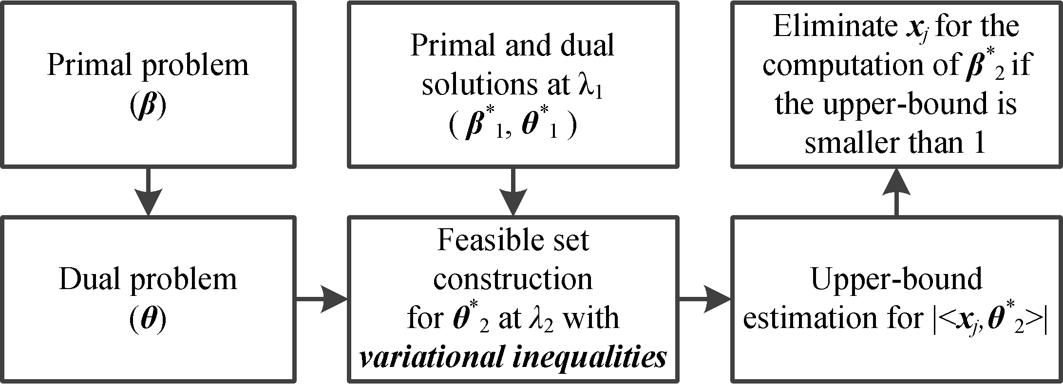
Figure 1: The work flow of the proposed Sasvi. The purpose is to discard the features that can be safely eliminated in computing $\bm{\beta}^{*}_{2}$ with the information obtained at $\lambda_{1}$.

The construction of a tight feasible set for $\bm{\theta}^{*}_{2}$ is key to the success of the screening technique. If the constructed feasible set is too loose, the estimated upper-bound of $|\langle\mathbf{x}_{j},\bm{\theta}^{*}_{2}\rangle|$ is over 1, and thus only a few features can be discarded. In this paper, we propose to construct the feasible set by using the variational inequalities that provide the sufficient and necessary optimality conditions for the dual problems with $\lambda=\lambda_{1}$ and $\lambda_{2}$. Then, we estimate the upper-bound of $|\langle\mathbf{x}_{j},\bm{\theta}^{*}_{2}\rangle|$ in the constructed feasbile set, and discard the $j$-th feature if the upper-bound is smaller than 1. For discussion convenience, we focus on Lasso in this paper, but the underlying methodology can be extended to the general problem in Eq. (1). Next, we elaborate the three building blocks that are illustrated in the bottom row of Figure 1.

2.1 The Dual Problem of Lasso

We follow the discussion in Section 6 of [9] in deriving the dual problem of Lasso as follows:

$$\min_{\bm{\beta}}\left[\frac{1}{2}\left\|X\bm{\beta}-\mathbf{y}\right\|_{2}^{2}+\lambda\|\bm{\beta}\|_{1}\right]$$ (6)

$$=\min_{\bm{\beta}}\max_{\bm{\theta}}\left[\langle\mathbf{y}-X\bm{\beta},\lambda\bm{\theta}\rangle-\frac{1}{2}\|\lambda\bm{\theta}\|_{2}^{2}+\lambda\|\bm{\beta}\|_{1}\right]$$

$$=\max_{\bm{\theta}}\min_{\bm{\beta}}\lambda\left[\langle\mathbf{y},\bm{\theta}\rangle-\frac{\lambda\|\bm{\theta}\|_{2}^{2}}{2}-\langle X^{T}\bm{\theta},\bm{\beta}\rangle+\|\bm{\beta}\|_{1}\right]$$

$$=\max_{\bm{\theta}:\|X^{T}\bm{\theta}\|_{\infty}\leq 1}\lambda^{2}\left[-\frac{1}{2}\left\|\bm{\theta}-\frac{\mathbf{y}}{\lambda}\right\|_{2}^{2}+\frac{1}{2}\left\|\frac{\mathbf{y}}{\lambda}\right\|_{2}^{2}\right].$$

A dual variable $\bm{\theta}$ is introduced in the first equality, and the equivalence can be verified by setting the derivative with regard to $\bm{\theta}$ to zero, which leads to the following relationship between the optimal primal variable ($\bm{\beta}^{*}$) and the optimal dual variable ($\bm{\theta}^{*}$):

$$\lambda\bm{\theta}^{*}=\mathbf{y}-X\bm{\beta}^{*}.$$ (7)

In obtaining the last equality of Eq. (6), we make use of the results to Eq. (2).

The dual problem of Eq. (1) can be formulated as:

$$\min_{\bm{\theta}:\|X^{T}\bm{\theta}\|_{\infty}\leq 1}\frac{1}{2}\left\|\bm{\theta}-\frac{\mathbf{y}}{\lambda}\right\|_{2}^{2}.$$ (8)

For Lasso, the $\lambda_{\max}$ in Eq. (5) can be analytically computed as $\lambda_{\max}=\|X^{T}\mathbf{y}\|_{\infty}$. In applying Sasvi, we might start with $\lambda_{1}=\lambda_{\max}$, since the primal and dual optimals can be computed analytically as: $\bm{\beta}_{1}^{*}=\mathbf{0}$ and $\bm{\theta}_{1}^{*}=\frac{\mathbf{y}}{\lambda_{\max}}$.

2.2 Feasible Set Construction

Given $\lambda_{1}$, $\bm{\theta}_{1}^{*}$ and $\lambda_{2}$, we aim at estimating the upper-bound of $|\langle\mathbf{x}_{j},\bm{\theta}^{*}_{2}\rangle|$ without the actual computation of $\bm{\theta}_{2}^{*}$. To this end, we construct a feasible set for $\bm{\theta}_{2}^{*}$, and then estimate the upper-bound in the constructed feasible set. To construct the feasible set, we make use of the variational inequality that provides the sufficient and necessary condition of a constrained convex optimization problem.

Lemma 1

[8] For the constrained convex optimization problem:

$$\min_{\mathbf{x}\in G}f(\mathbf{x}),$$ (9)

with $G$ being convex and closed and $f(\cdot)$ being convex and differentiable, $\mathbf{x}^{*}\in G$ is an optimal solution of Eq. (9) if and only if

$$\langle f^{\prime}(\mathbf{x}^{*}),\mathbf{x}-\mathbf{x}^{*}\rangle\geq 0,\forall\mathbf{x}\in G.$$ (10)

Eq. (10) is the so-called variation inequality for the problem in Eq. (9). Applying Lemma 1 to the Lasso dual problem in Eq. (8), we can represent the optimality conditions for $\bm{\theta}_{1}^{*}$ and $\bm{\theta}_{2}^{*}$ using the following two variational inequalities:

$$\left\langle\bm{\theta}_{1}^{*}-\frac{\mathbf{y}}{\lambda_{1}},\bm{\theta}-\bm{\theta}_{1}^{*}\right\rangle\geq 0,\forall\bm{\theta}:\|X^{T}\bm{\theta}\|_{\infty}\leq 1,$$ (11)

$$\left\langle\bm{\theta}_{2}^{*}-\frac{\mathbf{y}}{\lambda_{2}},\bm{\theta}-\bm{\theta}_{2}^{*}\right\rangle\geq 0,\forall\bm{\theta}:\|X^{T}\bm{\theta}\|_{\infty}\leq 1.$$ (12)

Plugging $\bm{\theta}=\bm{\theta}_{2}^{*}$ and $\bm{\theta}=\bm{\theta}_{1}^{*}$ into Eq. (11) and Eq. (12) respectively, we have

$$\left\langle\bm{\theta}_{1}^{*}-\frac{\mathbf{y}}{\lambda_{1}},\bm{\theta}_{2}^{*}-\bm{\theta}_{1}^{*}\right\rangle\geq 0,$$ (13)

$$\left\langle\bm{\theta}_{2}^{*}-\frac{\mathbf{y}}{\lambda_{2}},\bm{\theta}_{1}^{*}-\bm{\theta}_{2}^{*}\right\rangle\geq 0.$$ (14)

With Eq. (13) and Eq. (14), we can construct the following feasible set for $\bm{\theta}_{2}^{*}$ as:

$$\Omega(\bm{\theta}_{2}^{*})=\{\bm{\theta}:\langle\bm{\theta}_{1}^{*}-\frac{\mathbf{y}}{\lambda_{1}},\bm{\theta}-\bm{\theta}_{1}^{*}\rangle\geq 0,\langle\bm{\theta}-\frac{\mathbf{y}}{\lambda_{2}},\bm{\theta}_{1}^{*}-\bm{\theta}\rangle\geq 0\}.$$ (15)

For an illustration of the feasible set, please refer to Figure 2. Generally speaking, the closer $\lambda_{2}$ is to $\lambda_{1}$, the tighter the feasible set for $\bm{\theta}_{2}^{*}$ is. In fact, when $\lambda_{2}$ approaches to $\lambda_{1}$, $\Omega(\bm{\theta}_{2}^{*})$ concentrates to a singleton set that only contains $\bm{\theta}_{2}^{*}$. Note that one may use additional $\bm{\theta}$’s in Eq. (12) for improving the estimation of the feasible set of $\bm{\theta}_{2}^{*}$. Next, we discuss how to make use of the feasible set defined in Eq. (15) for estimating an upper-bound for $|\langle\mathbf{x}_{j},\bm{\theta}^{*}_{2}\rangle|$.

2.3 Upper-bound Estimation

Since $\bm{\theta}_{2}^{*}\in\Omega(\bm{\theta}_{2}^{*})$, we can estimate an upper-bound of $|\langle\mathbf{x}_{j},\bm{\theta}^{*}_{2}\rangle|$ by solving

$$\max_{\bm{\theta}\in\Omega(\bm{\theta}_{2}^{*})}|\langle\mathbf{x}_{j},\bm{\theta}\rangle|.$$ (16)

Next, we show how to solve Eq. (16). For discussion convenience, we introduce the following three variables:

$$\mathbf{a} =\frac{\mathbf{y}}{\lambda_{1}}-\bm{\theta}_{1}^{*}=\frac{X\bm{\beta}_{1}^{*}}{\lambda_{1}},$$ (17)

$$\mathbf{b} =\frac{\mathbf{y}}{\lambda_{2}}-\bm{\theta}_{1}^{*}=\mathbf{a}+(\frac{\mathbf{y}}{\lambda_{2}}-\frac{\mathbf{y}}{\lambda_{1}}),$$

$$\mathbf{r} =2\bm{\theta}-(\bm{\theta}_{1}^{*}+\frac{\mathbf{y}}{\lambda_{2}}),$$

where $\mathbf{a}$ denotes the prediction based on $\bm{\beta}_{1}^{*}$ scaled by $\frac{1}{\lambda_{1}}$, and $\mathbf{b}$ is the summation of $\mathbf{a}$ and the change of the inputs to the dual problem in Eq. (8) from $\lambda_{1}$ to $\lambda_{2}$.

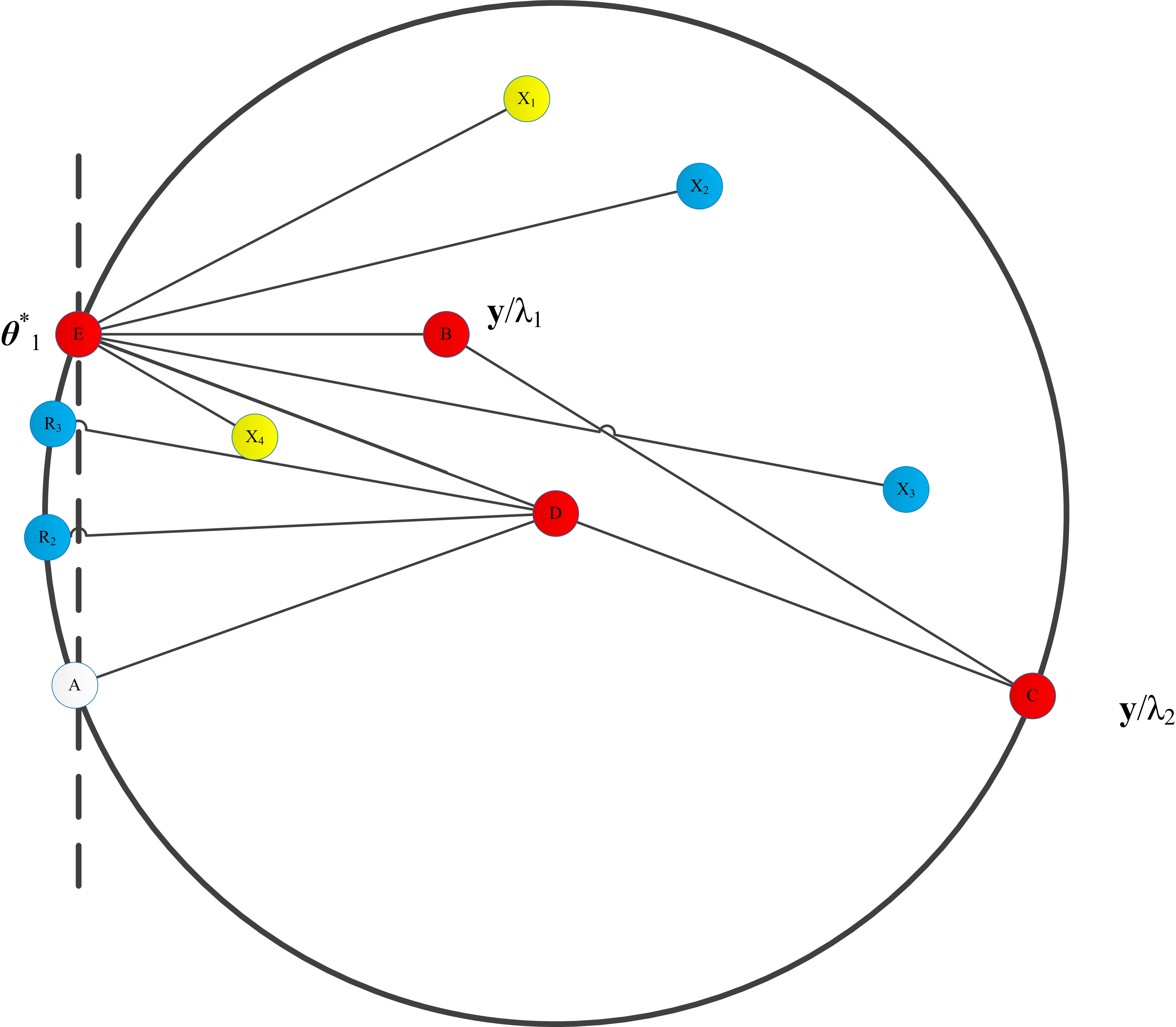
Figure 2: Illustration of the feasible set used in Sasvi and Theorem 3. The points in the figure are explained as follows. E: $\bm{\theta}_{1}^{*}$, B: $\frac{\mathbf{y}}{\lambda_{1}}$, C: $\frac{\mathbf{y}}{\lambda_{2}}$, D: $\frac{\bm{\theta}_{1}^{*}+\frac{\mathbf{y}}{\lambda_{2}}}{2}$. The left hand side of the dash line represents the half space $\{\bm{\theta}:\langle\bm{\theta}_{1}^{*}-\frac{\mathbf{y}}{\lambda_{1}},\bm{\theta}-\bm{\theta}_{1}^{*}\rangle\geq 0\}$, and the ball centered at D with radius ED represents $\{\bm{\theta}:\langle\bm{\theta}-\frac{\mathbf{y}}{\lambda_{2}},\bm{\theta}_{1}^{*}-\bm{\theta}\rangle\geq 0\}$. For Theorem 3, EX₁, EX₂, EX₃ and EX₄ denote $\pm\mathbf{x}_{j}$ in two subcases: 1) the angle between EB and EX₁ (EX₄) is larger than the angle between EB and EC, and 2) the angle between EB and EX₂ (EX₃) is smaller than the angle between EB and EC. R₂ (R₃) is the maximizer to Eq. (16) with EX₂ (EX₃) denoting $\pm\mathbf{x}_{j}$. With EX₁ (EX₄) denoting $\pm\mathbf{x}_{j}$, the maximizer to Eq. (16) is on the intersection between the dashed line and the ball centered at D with radius ED.

Figure 2 illustrates $\mathbf{a}$ and $\mathbf{b}$ by lines EB and EC, respectively. For the triangle EBC, the following theorem shows that the angle between $\mathbf{a}$ and $\mathbf{b}$ is acute.

Theorem 1

Let $\mathbf{y}\neq\mathbf{0}$, and $\|X^{T}\mathbf{y}\|_{\infty}\geq\lambda_{1}>\lambda_{2}>0$. We have

$$\mathbf{b}\neq\mathbf{0},\langle\mathbf{b},\mathbf{a}\rangle\geq 0,$$ (18)

and $\langle\mathbf{b},\mathbf{a}\rangle=0$ if and only if $\lambda_{1}=\|X^{T}\mathbf{y}\|_{\infty}$. In addition, if $\lambda_{1}<\|X^{T}\mathbf{y}\|_{\infty}$, then $\mathbf{a}\neq\mathbf{0}$.

The proof of Theorem 1 is given in Supplement A. With the notations in Eq. (17), Eq. (16) can be rewritten as

$$\max_{\mathbf{r}} \quad\frac{1}{2}\left|\left\langle\mathbf{x}_{j},\bm{\theta}_{1}^{*}+\frac{\mathbf{y}}{\lambda_{2}}\right\rangle+\langle\mathbf{x}_{j},\mathbf{r}\rangle\right|$$ (19)

subject to $$\quad\langle\mathbf{a},\mathbf{r}+\mathbf{b}\rangle\leq 0,\|\mathbf{r}\|_{2}^{2}\leq\|\mathbf{b}\|_{2}^{2}.$$

The objective function of Eq. (19) can be represented by half of the following form:

$$\max\left(\langle\mathbf{x}_{j},\bm{\theta}_{1}^{*}+\frac{\mathbf{y}}{\lambda_{2}}\rangle+\langle\mathbf{x}_{j},\mathbf{r}\rangle,-\langle\mathbf{x}_{j},\bm{\theta}_{1}^{*}+\frac{\mathbf{y}}{\lambda_{2}}\rangle-\langle\mathbf{x}_{j},\mathbf{r}\rangle\right)$$

which indicates that Eq. (19) can be computed by maximizing $\langle\mathbf{x}_{j},\mathbf{r}\rangle$ and $-\langle\mathbf{x}_{j},\mathbf{r}\rangle$ over the feasible set in the same equation. Maximizing $\langle\mathbf{x}_{j},\mathbf{r}\rangle$ and $-\langle\mathbf{x}_{j},\mathbf{r}\rangle$ can be computed by minimizing $\langle-\mathbf{x}_{j},\mathbf{r}\rangle$ and $\langle\mathbf{x}_{j},\mathbf{r}\rangle$, which can be solved by the following minimization problem:

$$\min_{\mathbf{r}} \quad\langle\mathbf{x},\mathbf{r}\rangle$$ (20)

subject to $$\quad\langle\mathbf{a},\mathbf{r}+\mathbf{b}\rangle\leq 0,\|\mathbf{r}\|_{2}^{2}\leq\|\mathbf{b}\|_{2}^{2}.$$

We assume that $\mathbf{x}$ is a non-zero vector. Let

$$\mathbf{x}^{\bot}=\mathbf{x}-\mathbf{a}\langle\mathbf{x},\mathbf{a}\rangle/\|\mathbf{a}\|_{2}^{2},$$ (21)

$$\mathbf{x}_{j}^{\bot}=\mathbf{x}_{j}-\mathbf{a}\langle\mathbf{x}_{j},\mathbf{a}\rangle/\|\mathbf{a}\|_{2}^{2},$$ (22)

$$\mathbf{y}^{\bot}=\mathbf{y}-\mathbf{a}\langle\mathbf{y},\mathbf{a}\rangle/\|\mathbf{a}\|_{2}^{2},$$ (23)

which are the orthogonal projections of $\mathbf{x}$, $\mathbf{x}_{j}$, and $\mathbf{y}$ onto the null space of $\mathbf{a}$, respectively. Our next theorem says that Eq. (20) admits a closed form solution.

Theorem 2

Let $0<\lambda_{1}\leq\|X^{T}\mathbf{y}\|_{\infty}$, $0<\lambda_{2}<\lambda_{1}$, $\mathbf{x}\neq\mathbf{0}$ and $\mathbf{y}\neq\mathbf{0}$. Eq. (20) equals to $-\|\mathbf{x}\|_{2}\|\mathbf{b}\|_{2}$, if $\frac{\langle\mathbf{b},\mathbf{a}\rangle}{\|\mathbf{b}\|_{2}}\leq\frac{\langle\mathbf{x},\mathbf{a}\rangle}{\|\mathbf{x}\|_{2}}$, and $-\|\mathbf{x}^{\bot}\|_{2}\sqrt{\|\mathbf{b}\|_{2}^{2}-\frac{\langle\mathbf{b},\mathbf{a}\rangle^{2}}{\|\mathbf{a}\|_{2}^{2}}}-\frac{\langle\mathbf{a},\mathbf{b}\rangle\langle\mathbf{x},\mathbf{a}\rangle}{\|\mathbf{a}\|_{2}^{2}}$ otherwise.

The proof of Theorem 2 is given in Supplement B. With Theorem 2, we can obtain the upper-bound of $|\langle\mathbf{x}_{j},\bm{\theta}^{*}_{2}\rangle|$ in the following theorem.

Theorem 3

Let $\mathbf{y}\neq 0$, and $\|X^{T}\mathbf{y}\|_{\infty}\geq\lambda_{1}>\lambda_{2}>0$. Denote

$$u_{j}^{+}(\lambda_{2})=\max_{\bm{\theta}\in\Omega(\bm{\theta}_{2}^{*})}\langle\mathbf{x}_{j},\bm{\theta}\rangle,$$ (24)

$$u_{j}^{-}(\lambda_{2})=\max_{\bm{\theta}\in\Omega(\bm{\theta}_{2}^{*})}\langle-\mathbf{x}_{j},\bm{\theta}\rangle.$$ (25)

We have:

1) If $\mathbf{a}\neq\mathbf{0}$ and $\frac{\langle\mathbf{b},\mathbf{a}\rangle}{\|\mathbf{b}\|_{2}\|\mathbf{a}\|_{2}}>\frac{|\langle\mathbf{x}_{j},\mathbf{a}\rangle|}{\|\mathbf{x}_{j}\|_{2}\|\mathbf{a}\|_{2}}$ then

$$u_{j}^{+}(\lambda_{2})=\langle\mathbf{x}_{j},\bm{\theta}_{1}^{*}\rangle+\frac{\frac{1}{\lambda_{2}}-\frac{1}{\lambda_{1}}}{2}\left[\|\mathbf{x}_{j}^{\bot}\|_{2}\|\mathbf{y}^{\bot}\|_{2}+\langle\mathbf{x}_{j}^{\bot},\mathbf{y}^{\bot}\rangle\right],$$ (26)

$$u_{j}^{-}(\lambda_{2})=-\langle\mathbf{x}_{j},\bm{\theta}_{1}^{*}\rangle+\frac{\frac{1}{\lambda_{2}}-\frac{1}{\lambda_{1}}}{2}\left[\|\mathbf{x}_{j}^{\bot}\|_{2}\|\mathbf{y}^{\bot}\|_{2}-\langle\mathbf{x}_{j}^{\bot},\mathbf{y}^{\bot}\rangle\right].$$ (27)

2) If $\langle\mathbf{x}_{j},\mathbf{a}\rangle>0$ and $\frac{\langle\mathbf{b},\mathbf{a}\rangle}{\|\mathbf{b}\|_{2}\|\mathbf{a}\|_{2}}\leq\frac{\langle\mathbf{x}_{j},\mathbf{a}\rangle}{\|\mathbf{x}_{j}\|_{2}\|\mathbf{a}\|_{2}}$, then $u_{j}^{+}(\lambda_{2})$ satisfies Eq. (26), and

$$u_{j}^{-}(\lambda_{2})=-\langle\mathbf{x}_{j},\bm{\theta}_{1}^{*}\rangle+\frac{1}{2}\left[\|\mathbf{x}_{j}\|_{2}\|\mathbf{b}\|_{2}-\langle\mathbf{x}_{j},\mathbf{b}\rangle\right].$$ (28)

3) If $\langle\mathbf{x}_{j},\mathbf{a}\rangle<0$ and $\frac{\langle\mathbf{b},\mathbf{a}\rangle}{\|\mathbf{b}\|_{2}\|\mathbf{a}\|_{2}}\leq\frac{-\langle\mathbf{x}_{j},\mathbf{a}\rangle}{\|\mathbf{x}_{j}\|_{2}\|\mathbf{a}\|_{2}}$, then

$$u_{j}^{+}(\lambda_{2})=\langle\mathbf{x}_{j},\bm{\theta}_{1}^{*}\rangle+\frac{1}{2}\left[\|\mathbf{x}_{j}\|_{2}\|\mathbf{b}\|_{2}+\langle\mathbf{x}_{j},\mathbf{b}\rangle\right].$$ (29)

and $u_{j}^{-}(\lambda_{2})$ satisfies Eq. (27).

4) If $\mathbf{a}=\mathbf{0}$, then Eq. (28) and Eq. (29) hold.

The proof of Theorem 3 is given in Supplement C. An illustration of Theorem 3 for different cases can be found in Figure 2. It follows from Eq. (4) that, if $u_{j}^{+}(\lambda_{2})<1$ and $u_{j}^{-}(\lambda_{2})<1$, then the $j$-th feature can be safely eliminated for the computation of $\bm{\beta}_{2}^{*}$. We provide the following analysis to the established upper-bound. Firstly, we have

$$\lim_{\lambda_{2}\rightarrow\lambda_{1}}u_{j}^{+}(\lambda_{2})=\langle\mathbf{x}_{j},\bm{\theta}_{1}^{*}\rangle,\lim_{\lambda_{2}\rightarrow\lambda_{1}}u_{j}^{-}(\lambda_{2})=-\langle\mathbf{x}_{j},\bm{\theta}_{1}^{*}\rangle,$$

which attributes to the fact that $\lim_{\lambda_{2}\rightarrow\lambda_{1}}\Omega(\bm{\theta}_{2}^{*})=\{\bm{\theta}_{1}^{*}\}$. Secondly, in the extreme case that $\mathbf{x}_{j}$ is orthogonal to the scaled prediction $\mathbf{a}=\frac{X\bm{\beta}_{1}^{*}}{\lambda_{1}}$ which is nonzero, Theorem 3 leads to $\mathbf{x}_{j}^{\bot}=\mathbf{0}$, $u_{j}^{+}(\lambda_{2})=\langle\mathbf{x}_{j},\bm{\theta}_{1}^{*}\rangle$ and $u_{j}^{-}(\lambda_{2})=-\langle\mathbf{x}_{j},\bm{\theta}_{1}^{*}\rangle$. Thus, the $j$-th feature can be safely removed for any positive $\lambda_{2}$ that is smaller than $\lambda_{1}$ so long as $|\langle\mathbf{x}_{j},\bm{\theta}_{1}^{*}\rangle|<1$. Thirdly, in the case that $\mathbf{x}_{j}$ has low correlation with the prediction $\mathbf{a}=\frac{X\bm{\beta}_{1}^{*}}{\lambda_{1}}$, Theorem 3 indicates that the $j$-th feature is very likely to be safely removed for a wide range of $\lambda_{2}$ if $|\langle\mathbf{x}_{j},\bm{\theta}_{1}^{*}\rangle|<1$. The monotone properties of the upper-bound established in Theorem 3 is given Section 4.

3 Comparison with Existing Approaches

Our proposed Sasvi differs from the existing screening techniques [5, 13, 14, 15] in the construction of the feasible set for $\bm{\theta}_{2}^{*}$.

3.1 Comparison with the Strong Rule

The strong rule [13] works on $0<\lambda_{2}<\lambda_{1}$ and makes use of the assumption

$$|\lambda_{2}\langle\mathbf{x}_{j},\bm{\theta}_{2}^{*}\rangle-\lambda_{1}\langle\mathbf{x}_{j},\bm{\theta}_{1}^{*}\rangle|\leq|\lambda_{2}-\lambda_{1}|,$$ (30)

from which we can obtain an estimated upper-bound for $|\langle\mathbf{x}_{j},\bm{\theta}_{2}^{*}\rangle|$ as:

$$|\langle\mathbf{x}_{j},\bm{\theta}_{2}^{*}\rangle| \leq\frac{|\lambda_{1}\langle\mathbf{x}_{j},\bm{\theta}_{1}^{*}\rangle|+|\lambda_{2}\langle\mathbf{x}_{j},\bm{\theta}_{2}^{*}\rangle-\lambda_{1}\langle\mathbf{x}_{j},\bm{\theta}_{1}^{*}\rangle|}{\lambda_{2}}$$ (31)

$$\leq\frac{|\lambda_{1}\langle\mathbf{x}_{j},\bm{\theta}_{1}^{*}\rangle|+(\lambda_{1}-\lambda_{2})}{\lambda_{2}}$$

$$=\frac{\lambda_{1}}{\lambda_{2}}|\langle\mathbf{x}_{j},\bm{\theta}_{1}^{*}\rangle|+\left[\frac{\lambda_{1}}{\lambda_{2}}-1\right]$$

A comparison between Eq. (31) and the upper-bound established in Theorem 3 shows that, 1) both are dependent on $\langle\mathbf{x}_{j},\bm{\theta}_{1}^{*}\rangle$, the inner product between the $j$-th feature and the dual variable $\bm{\theta}_{1}^{*}$ obtained at $\lambda_{1}$, but note that $\frac{\lambda_{1}}{\lambda_{2}}>1$, 2) in comparison with the data independent term $\frac{\lambda_{1}}{\lambda_{2}}-1$ used in the strong rule, Sasvi utilizes a data dependent term as shown in Eqs. (26)-(29). We note that, 1) when a feature $\mathbf{x}_{j}$ has low correlation with the prediction $\mathbf{a}=\frac{X\bm{\beta}_{1}^{*}}{\lambda_{1}}$, the upper-bound for $|\langle\mathbf{x}_{j},\bm{\theta}_{2}^{*}\rangle|$ estimated by Sasvi might be lower than the one by the strong rule , and 2) as pointed out in [13], Eq. (30) might not always hold, and the same applies to Eq. (31).

Next, we compare Sasvi with the SAFE approach [5] and the DPP approach [14], and the differences in terms of the feasible sets are shown in Figure 3.

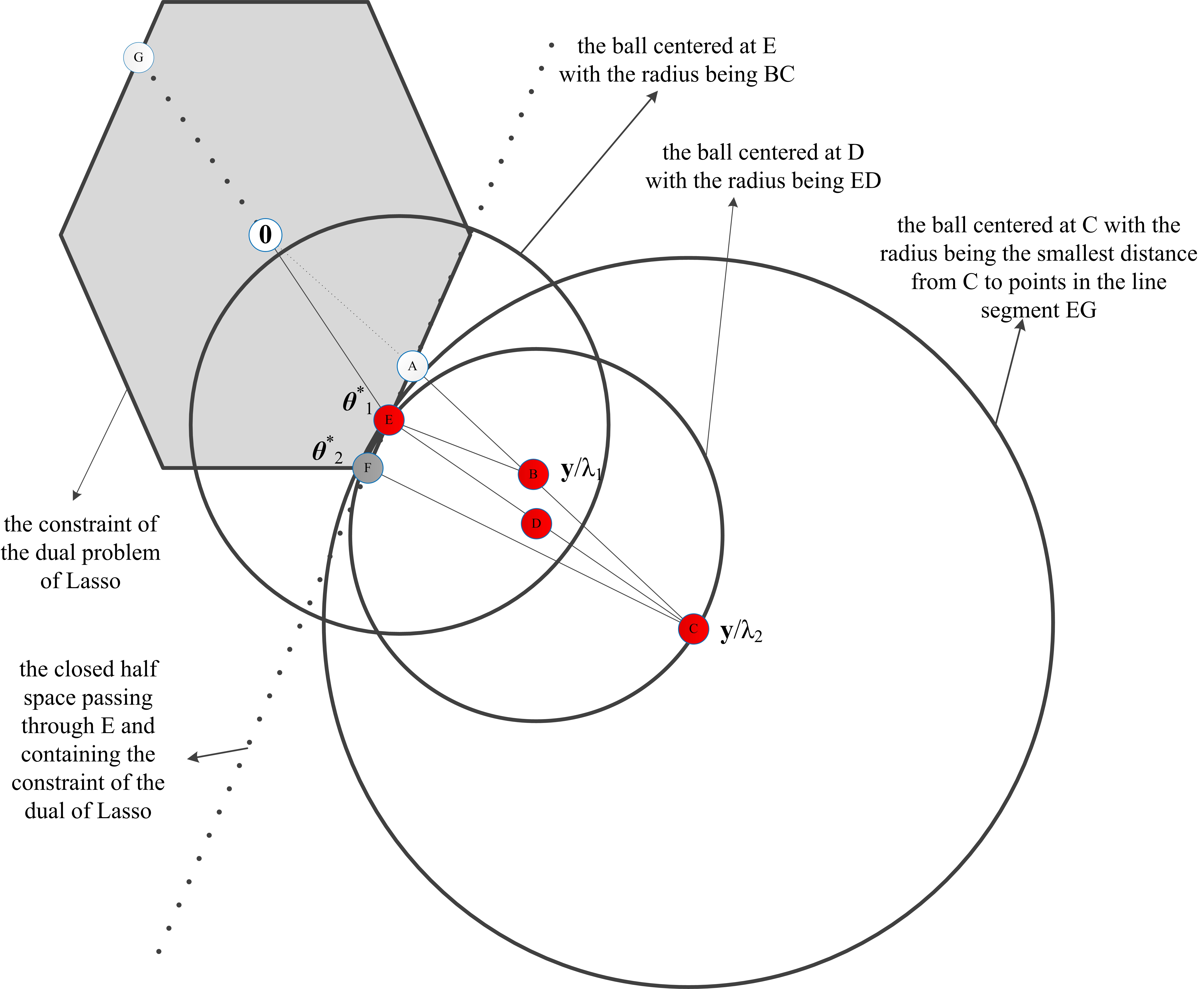
Figure 3: Comparison of Sasvi with existing safe screening approaches. The points in the figure are as follows. A: $\frac{\mathbf{y}}{\lambda_{\max}}$, B: $\frac{\mathbf{y}}{\lambda_{1}}$, C: $\frac{\mathbf{y}}{\lambda_{2}}$, D: the middle point of C and E, E: $\bm{\theta}_{1}^{*}$, F: $\bm{\theta}_{2}^{*}$, and G: $-\bm{\theta}_{1}^{*}$. The feasible set for $\bm{\theta}_{2}^{*}$ used by the proposed Sasvi approach is the intersection between the ball centered at D with radius being half EC and the closed half space passing through E and containing the constraint of the dual of Lasso. The feasible set for $\bm{\theta}_{2}^{*}$ used by the SAFE [5] approach is the ball centered at C with radius being the smallest distance from C to the points in the line segment EG. The feasible set for $\bm{\theta}_{2}^{*}$ used by the DPP [14] approach is the ball centered at E with radius BC.

3.2 Comparison with the SAFE approach

Denote $G(\bm{\theta})=\frac{1}{2}\|\mathbf{y}||_{2}^{2}-\frac{1}{2}\|\lambda_{2}\bm{\theta}-\mathbf{y}||_{2}^{2}$. The SAFE approach makes use of the so-called “dual” scaling, and compute the upper-bound of the $G(\bm{\theta})$ for $\lambda_{2}$ as

$$\gamma(\lambda_{2})=\max_{s:|s|\leq 1}G(s\bm{\theta})=\max_{s:|s|\leq 1}\frac{1}{2}\|\mathbf{y}||_{2}^{2}-\frac{1}{2}\|s\lambda_{2}\bm{\theta}_{1}^{*}-\mathbf{y}||_{2}^{2},$$ (32)

Note that, compared to the SAFE paper, the dual variable $\bm{\theta}$ has been scaled in the formulation in Eq. (32), but this scaling does not influence of the following result for the SAFE approach. Denote $s^{*}$ as the optimal solution. Solving Eq. (32), we have $s^{*}=\max\left(\min\left(\frac{\langle\bm{\theta}_{1}^{*},\mathbf{y}\rangle}{\lambda_{2}\|\bm{\theta}_{1}^{*}\|_{2}},1\right),-1\right)$ when $\bm{\theta}_{1}\neq\mathbf{0}$. The SAFE approach computes the upper-bound for $|\langle\mathbf{x}_{j},\bm{\theta}_{2}^{*}\rangle|$ as follows:

$$|\langle\mathbf{x}_{j},\bm{\theta}_{2}^{*}\rangle| \leq\max_{\bm{\theta}:G(\bm{\theta})\geq\gamma(\lambda_{2})}|\langle\mathbf{x}_{j},\bm{\theta}\rangle|$$ (33)

$$=\max_{\bm{\theta}:\|\bm{\theta}-\frac{\mathbf{y}}{\lambda_{2}}||_{2}\leq\|s^{*}\bm{\theta}_{1}^{*}-\frac{\mathbf{y}}{\lambda_{2}}||_{2}}|\langle\mathbf{x}_{j},\bm{\theta}\rangle|$$

$$=\frac{|\langle\mathbf{x}_{j},\mathbf{y}\rangle|}{\lambda_{2}}+\|\mathbf{x}_{j}\|_{2}\left\|s^{*}\bm{\theta}_{1}^{*}-\frac{\mathbf{y}}{\lambda_{2}}\right\|_{2}.$$

Next, we show that the feasible set for $\bm{\theta}_{2}^{*}$ used in Eq. (33) can be derived from the variational inequality in Eq. (12) followed by relaxations.

Utilizing $\|X^{T}\bm{\theta}_{1}^{*}\|_{\infty}\leq 1$ and $|s^{*}|\leq 1$, we can set $\bm{\theta}=s^{*}\bm{\theta}_{1}^{*}$ in Eq. (12) and obtain

$$\left\langle\bm{\theta}_{2}^{*}-\frac{\mathbf{y}}{\lambda_{2}},s^{*}\bm{\theta}_{1}^{*}-\bm{\theta}_{2}^{*}\right\rangle\geq 0,$$ (34)

which leads to

$$\left\langle\bm{\theta}_{2}^{*}-\frac{\mathbf{y}}{\lambda_{2}},\bm{\theta}_{2}^{*}-\frac{\mathbf{y}}{\lambda_{2}}\right\rangle-\left\langle\bm{\theta}_{2}^{*}-\frac{\mathbf{y}}{\lambda_{2}},s^{*}\bm{\theta}_{1}^{*}-\frac{\mathbf{y}}{\lambda_{2}}\right\rangle$$ (35)

$$=\left\langle\bm{\theta}_{2}^{*}-\frac{\mathbf{y}}{\lambda_{2}},\bm{\theta}_{2}^{*}-\frac{\mathbf{y}}{\lambda_{2}}+\frac{\mathbf{y}}{\lambda_{2}}-s^{*}\bm{\theta}_{1}^{*}\right\rangle\leq 0.$$

Since

$$\left\langle\bm{\theta}_{2}^{*}-\frac{\mathbf{y}}{\lambda_{2}},s^{*}\bm{\theta}_{1}^{*}-\frac{\mathbf{y}}{\lambda_{2}}\right\rangle\leq\left\|\bm{\theta}_{2}^{*}-\frac{\mathbf{y}}{\lambda_{2}}\right\|_{2}\left\|s^{*}\bm{\theta}_{1}^{*}-\frac{\mathbf{y}}{\lambda_{2}}\right\|_{2},$$ (36)

we have

$$\left\|\bm{\theta}_{2}^{*}-\frac{\mathbf{y}}{\lambda_{2}}\right\|_{2}\leq\left\|s^{*}\bm{\theta}_{1}^{*}-\frac{\mathbf{y}}{\lambda_{2}}\right\|_{2},$$ (37)

which is the feasible set used in Eq. (33). Note that, the ball defined by Eq. (37) has higher volume than the one defined by Eq. (34) due to the relaxation used in Eq. (36), and it can be shown that the ball defined by Eq. (34) lies within the ball defined by Eq. (37).

3.3 Comparison with the DPP approach

The feasible set for $\bm{\theta}_{2}^{*}$ used in the DPP approach is

$$\left\|\frac{\mathbf{y}}{\lambda_{2}}-\frac{\mathbf{y}}{\lambda_{1}}\right\|_{2}\geq\left\|\bm{\theta}_{2}^{*}-\bm{\theta}_{1}^{*}\right\|_{2},$$ (38)

which can be obtained by

$$\left\langle\frac{\mathbf{y}}{\lambda_{2}}-\frac{\mathbf{y}}{\lambda_{1}},\bm{\theta}_{2}^{*}-\bm{\theta}_{1}^{*}\right\rangle\geq\langle\bm{\theta}_{2}^{*}-\bm{\theta}_{1}^{*},\bm{\theta}_{2}^{*}-\bm{\theta}_{1}^{*}\rangle.$$ (39)

and

$$\left\langle\frac{\mathbf{y}}{\lambda_{2}}-\frac{\mathbf{y}}{\lambda_{1}},\bm{\theta}_{2}^{*}-\bm{\theta}_{1}^{*}\right\rangle\leq\left\|\frac{\mathbf{y}}{\lambda_{2}}-\frac{\mathbf{y}}{\lambda_{1}}\right\|_{2}\|\bm{\theta}_{2}^{*}-\bm{\theta}_{1}^{*}\|_{2},$$ (40)

where Eq. (39) is a result of adding Eq. (13) and Eq. (14). Therefore, although the authors in [14] motivates the DPP approach from the viewpoint of Euclidean projection, the DPP approach can indeed be treated as generating the feasible set for $\bm{\theta}_{2}^{*}$ using the variational inequality in Eq. (11) and Eq. (12) followed by relaxation in Eq. (40). Note that, the ball specified by Eq. (38) has higher volume than the one specified by Eq. (39) due to the relaxation used in Eq. (40), and it can be shown that the ball defined by Eq. (39) lies within the ball defined by Eq. (38).

4 Feature Sure Removal Parameter

In this subsection, we study the monotone properties of the upper-bound established in Theorem 3 with regard to the regularization parameter $\lambda_{2}$. With such study, we can identify the feature sure removal parameter—the smallest value of $\lambda$ above which a feature is guaranteed to have zero coefficient and thus can be safely removed.

Without loss of generality, we assume $\langle\mathbf{x}_{j},\mathbf{a}\rangle\geq 0$ and the results can be easily extended to the case $\langle\mathbf{x}_{j},\mathbf{a}\rangle<0$. In addition, we assume that if $\lambda_{1}\neq\|X^{T}\mathbf{y}\|_{\infty}$ then $\bm{\theta}_{1}^{*}\neq\frac{\mathbf{y}}{\|X^{T}\mathbf{y}\|_{\infty}}$. This is a valid assumption for real data.

Let $\mathbf{y}\neq 0$, and $\lambda_{\max}=\|X^{T}\mathbf{y}\|_{\infty}\geq\lambda_{1}\geq\lambda>0$. We introduce the following two auxiliary functions:

$$f(\lambda)=\frac{\langle\frac{\mathbf{y}}{\lambda}-\bm{\theta}_{1}^{*},\mathbf{a}\rangle}{\|\frac{\mathbf{y}}{\lambda}-\bm{\theta}_{1}^{*}\|_{2}}$$ (41)

$$g(\lambda)=\frac{\langle\frac{\mathbf{y}}{\lambda}-\bm{\theta}_{1}^{*},\mathbf{y}\rangle}{\|\frac{\mathbf{y}}{\lambda}-\bm{\theta}_{1}^{*}\|_{2}}$$ (42)

We show in Supplement D that $f(\lambda)$ is strictly increasing with regard to $\lambda$ in $(0,\lambda_{1}]$ and $g(\lambda)$ is strictly decreasing with regard to $\lambda$ in $(0,\lambda_{1}]$. Such monotone properties, which are illustrated geometrically in the first plot of Figure 4, guarantee that $f(\lambda)=\frac{\langle\mathbf{x}_{j},\mathbf{a}\rangle}{\|\mathbf{x}_{j}\|_{2}}$ and $g(\lambda)=\frac{\langle\mathbf{x}_{j},\mathbf{y}\rangle}{\|\mathbf{x}_{j}\|_{2}}$ have unique roots with regard to $\lambda$ when some conditions are satisfied.

Our main results are summarized in the following theorem:

Theorem 4

Let $\mathbf{y}\neq 0$ and $\|X^{T}\mathbf{y}\|_{\infty}\geq\lambda_{1}>\lambda_{2}>0$. Let $\langle\mathbf{x}_{j},\mathbf{a}\rangle\geq 0$. Assume that if $\lambda_{1}\neq\|X^{T}\mathbf{y}\|_{\infty}$ then $\bm{\theta}_{1}^{*}\neq\frac{\mathbf{y}}{\|X^{T}\mathbf{y}\|_{\infty}}$.

Define $\lambda_{2,a}$ as follows: If $\frac{\langle\mathbf{y},\mathbf{a}\rangle}{\|\mathbf{y}\|_{2}}\geq\frac{\langle\mathbf{x}_{j},\mathbf{a}\rangle}{\|\mathbf{x}_{j}\|_{2}}$, then let $\lambda_{2,a}=0$; otherwise, let $\lambda_{2,a}$ be the unique value in $(0,\lambda_{1}]$ that satisfies $f(\lambda_{2,a})=\frac{\langle\mathbf{x}_{j},\mathbf{a}\rangle}{\|\mathbf{x}_{j}\|_{2}}$.

Define $\lambda_{2,y}$ as follows: If $\mathbf{a}=\mathbf{0}$ or if $\mathbf{a}\neq\mathbf{0}$ and $\frac{\langle\mathbf{a},\mathbf{y}\rangle}{\|\mathbf{a}\|_{2}}\geq\frac{\langle\mathbf{x}_{j},\mathbf{y}\rangle}{\|\mathbf{x}_{j}\|_{2}}$, then let $\lambda_{2,y}=\lambda_{1}$; otherwise, let $\lambda_{2,y}$ be the unique value in $(0,\lambda_{1}]$ that satisfies $g(\lambda_{2,y})=\frac{\langle\mathbf{x}_{j},\mathbf{y}\rangle}{\|\mathbf{x}_{j}\|_{2}}$.

We have the following monotone properties:

• $u_{j}^{+}(\lambda_{2})$ is monotonically decreasing with regard to $\lambda_{2}$ in $(0,\lambda_{1}]$.

• If $\lambda_{2,a}\leq\lambda_{2,y}$, then $u_{j}^{-}(\lambda_{2})$ is monotonically decreasing with regard to $\lambda_{2}$ in $(0,\lambda_{1}]$.

• If $\lambda_{2,a}>\lambda_{2,y}$, then $u_{j}^{-}(\lambda_{2})$ is monotonically decreasing with regard to $\lambda_{2}$ in $(0,\lambda_{2,y})$ and $(\lambda_{2,a},\lambda_{1})$, but monotonically increasing with regard to $\lambda_{2}$ in $[\lambda_{2,y},\lambda_{2,a}]$.

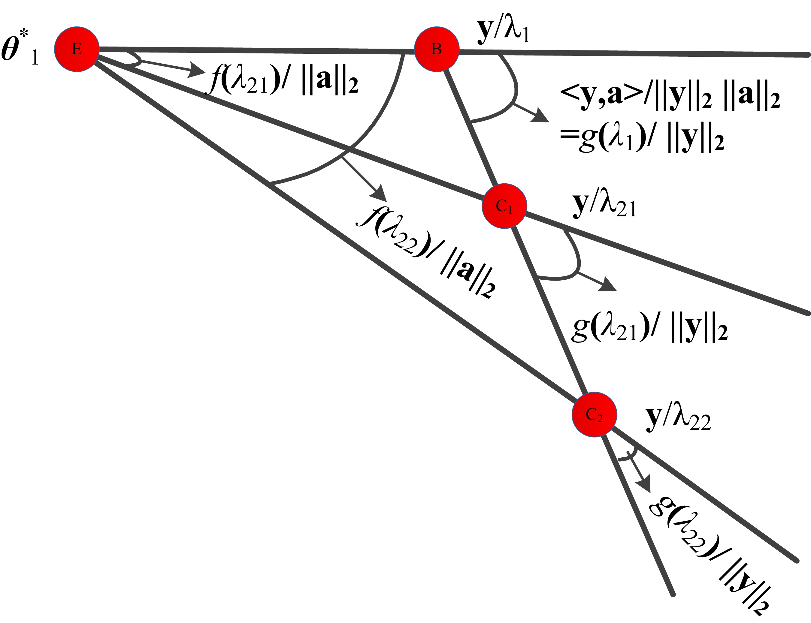
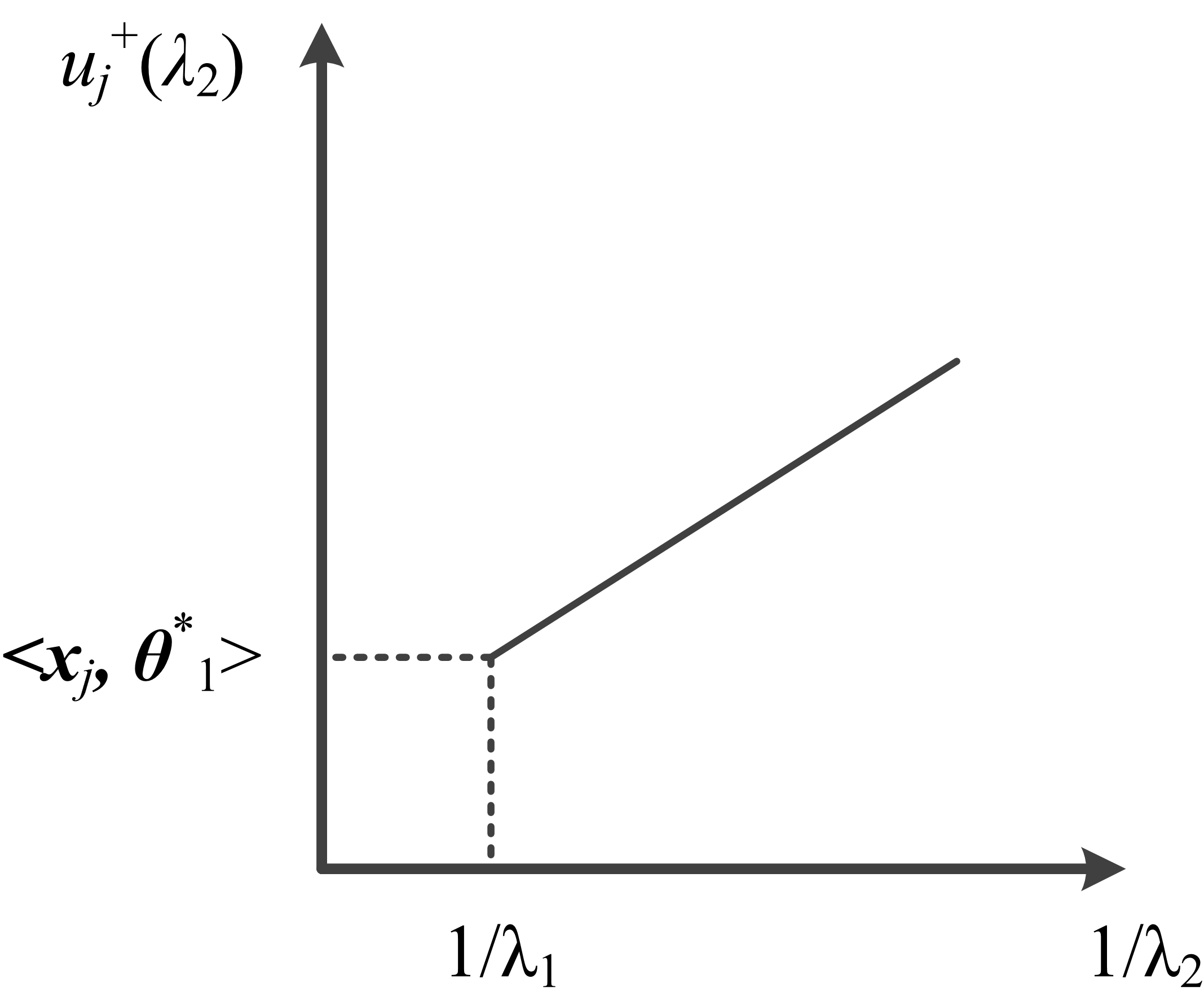
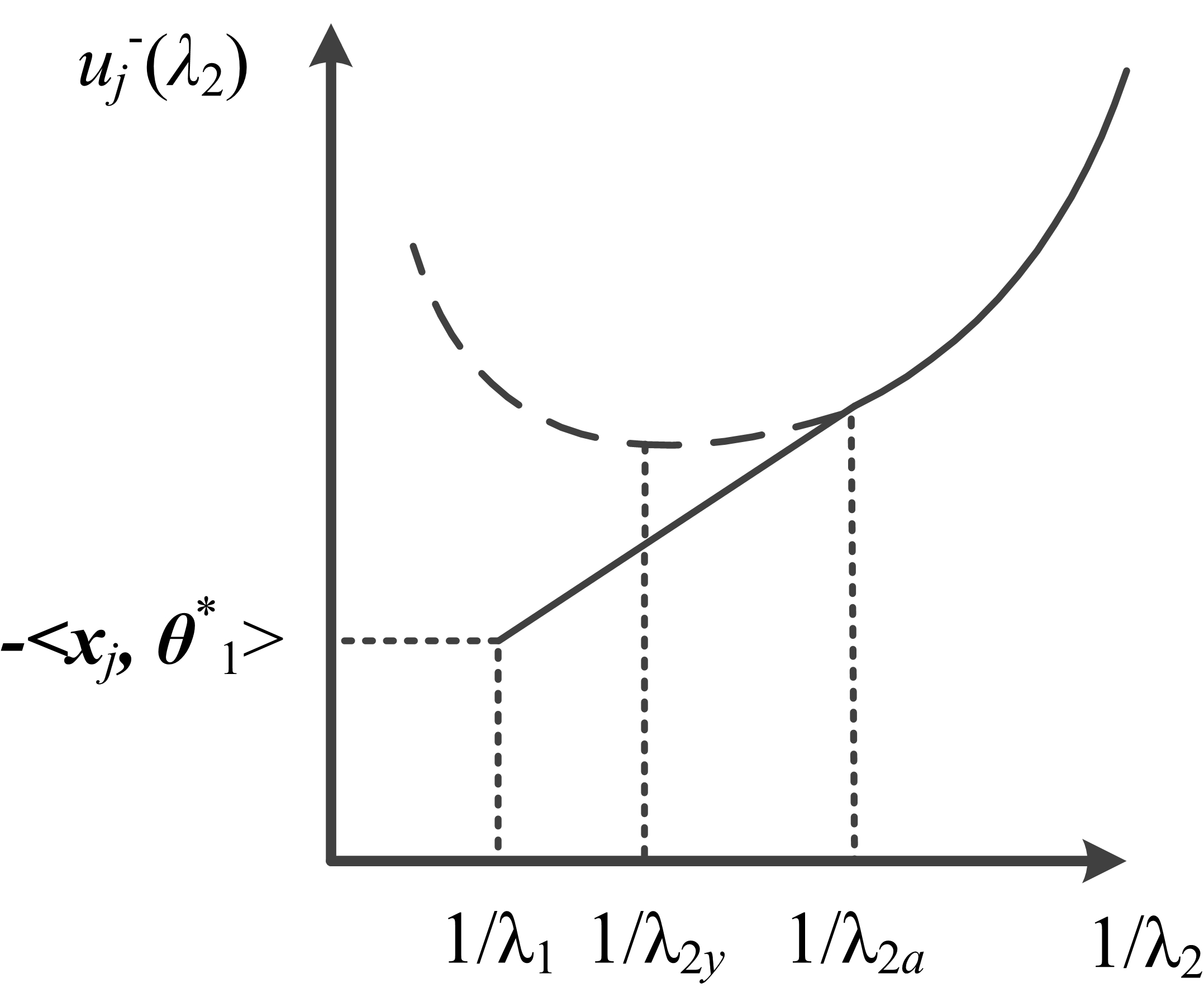
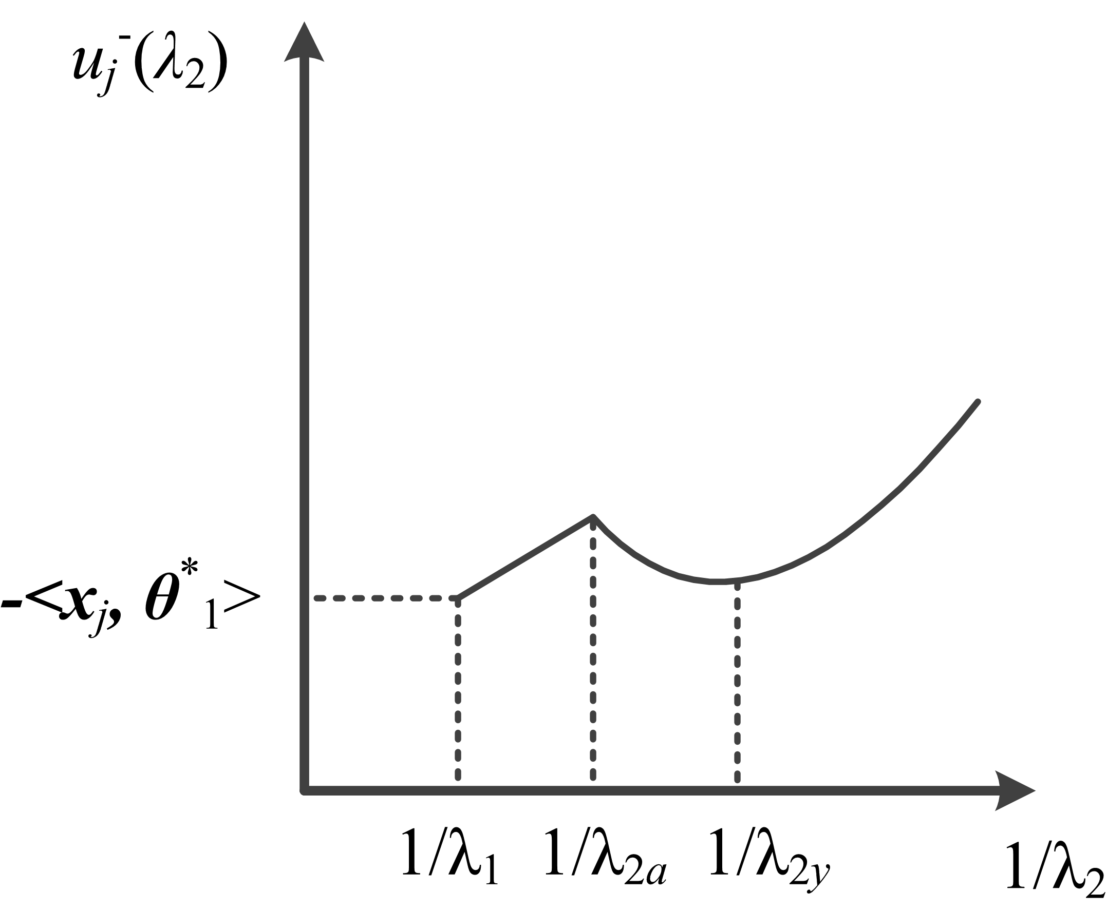
Figure 4: Illustration of the monotone properties of Sasvi for Lasso with the assumption $\langle\mathbf{x}_{j},\mathbf{a}\rangle\geq 0$. The first plot geometrically shows the monotone properties of $f(\lambda)$ and $g(\lambda)$, respectively. The last three plots correspond to the three cases in Theorem 4. For illustration convenience, the x-axis denotes $\frac{1}{\lambda_{2}}$ rather than $\lambda_{2}$.

The proof of Theorem 4 is given in Supplement D. Note that, $\lambda_{2,a}$ and $\lambda_{2,y}$ are dependent on the index $j$, which is omitted for discussion convenience. Figure 4 illustrates results presented in Theorem 4. The first two cases of Theorem 4 indicate that, if the $j$-th feature $\mathbf{x}_{j}$ can be safely removed for a regularization parameter $\lambda=\lambda_{2}$, then it can also be safely discarded for any regularization parameter $\lambda$ larger than $\lambda_{2}$. However, the third case in Theorem 4 says that this is not always true. This somehow coincides with the characteristic of Lasso that, a feature that is inactive for a regularization parameter $\lambda=\lambda_{2}$ might become active for a larger regularization parameter $\lambda>\lambda_{2}$. In other words, when following the Lasso solution path with a decreasing regularization parameter, a feature that enters into the model might get removed.

By using Theorem 4, we can easily identify for each feature a sure removable parameter $\lambda_{s}$ that satisfies $u_{j}^{+}(\lambda)<1$ and $u_{j}^{-}(\lambda)<1$, $\forall\lambda>\lambda_{s}$. Note that Theorem 4 assumes $\langle\mathbf{x}_{j},\mathbf{a}\rangle\geq 0$, but it can be easily extended to the case $\langle\mathbf{x}_{j},\mathbf{a}\rangle<0$ by replacing $\mathbf{x}_{j}$ with $-\mathbf{x}_{j}$.

5 Experiment

In this section, we conduct experiments to evaluate the performance of the proposed Sasvi in comparison with the sequential SAFE rule [5], the sequential strong rule [13], and the sequential DPP [14]. Note that, SAFE, Sasvi and DPP methods are “safe” in the sense that the discarded features are guaranteed to have 0 coefficients in the true solution, and the strong rule—which is a heuristic rule—might make error and such error was corrected by a KKT condition check as suggested in [13].

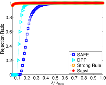
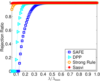
(Real: MNIST)            (Real: PIE)

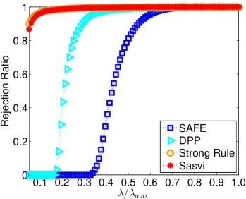
(Synthetic, $\bar{p}=100$)      (Synthetic, $\bar{p}=1000$)

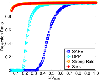
(Synthetic, $\bar{p}=5000$)

Figure 5: The rejectioin ratios—the ratios of the number features screened out by SAFE, DPP, the strong rule and Sasvi on synthetic and real data sets.

Synthetic Data Set We follow [1, 16, 12] in simulating the data as follows:

$$\mathbf{y}=X\bm{\beta}^{*}+\sigma\bm{\epsilon},\quad\bm{\epsilon}\sim N(0,1),$$ (43)

where $X$ has $250\times 10000$ entries. Similar to [1, 16, 12], we set the pairwise correlation between the $i$-th feature and the $j$-th feature to $0.5^{|i-j|}$ and draw $X$ from a Gaussian distribution. In constructing the ground truth $\bm{\beta}^{*}$, we set the number of non-zero components to $\bar{p}$ and randomly assign the values from a uniform $[-1,1]$ distribution. We set $\sigma=0.1$ and generate the response vector $\mathbf{y}\in\mathbb{R}^{250}$ using Eq. (43). For the value of $\bar{p}$, we try 100, 1000, and 5000.

PIE Face Image Data Set The PIE face image data set used in this experiment  contains $11554$ gray face images of $68$ people, taken under different poses, illumination conditions and expressions. Each of the images has $32\times 32$ pixels. To use the regression model in Eq. (43), we first randomly pick up an image as the response $\mathbf{y}\in\mathbb{R}^{1024}$, and then set the remaining images as the data matrix $X\in\mathbb{R}^{1024\times 11553}$.

MNIST Handwritten Digit Data Set This data set contains grey images of scanned handwritten digits, including $60,000$ for training and $10,000$ for testing. The dimension of each image is $28\times 28$. To use the regression model in Eq. (43), we first randomly select $5000$ images for each digit from the training set (and in total we have $50000$ images) and get a data matrix $X\in\mathbb{R}^{784\times 50000}$, and then we randomly select an image from the testing set and treat it as the response vector $\mathbf{y}\in\mathbb{R}^{784}$.

Experimental Settings For the Lasso solver, we make use of the SLEP package [7]. For a given generated data set ($X$ and $\mathbf{y}$), we run the solver with or without screening rules to solve the Lasso problems along a sequence of $100$ parameter values equally spaced on the $\lambda/\lambda_{max}$ scale from $0.05$ to $1.0$. The reported results are averaged over $100$ trials of randomly drawn $X$ and $\mathbf{y}$.

Method	Synthetic with $\bar{p}$			Real
	100	1000	5000	MINST	PIE
solver	88.55	101.00	101.55	2683.57	617.85
SAFE	73.37	88.42	90.21	651.23	128.54
DPP	44.00	49.57	50.15	328.47	79.84
Strong	2.53	3.00	2.92	5.57	2.97
Sasvi	2.49	2.77	2.76	5.02	1.90

Table 1: Running time (in seconds) for solving the Lasso problems along a sequence of $100$ tuning parameter values equally spaced on the scale of ${\lambda}/{\lambda_{max}}$ from $0.05$ to $1$ by the solver [7] without screening, and the solver combined with different screening methods.

Results Table 1 reports the running time by different screening rules, and Figure 5 presents the corresponding rejection ratios—the ratios of the number features screened out by the screening approaches. It can be observed that the propose Sasvi significantly outperforms the safe screening rules such as SAFE and DPP. The reason is that, Sasvi is able to discard more inactive features as discussed in Section 3. In addition, the rejection ratios of the strong rule and Sasvi are comparable, and both of them are more effective in discarding inactive features than SAFE and DPP. In terms of the speedup, Sasvi provides better performance than the strong rule. The reason is that the strong rule is a heuristic screening method, i.e., it may mistakenly discard active features which have nonzero components in the solution, and thus the strong rule needs to check the KKT conditions to make correction if necessary to ensure the correctness of the result. In contrast, Sasvi does not need to check the KKT conditions or make correction since the discarded features are guaranteed to be absent from the resulting sparse representation.

6 Conclusion

The safe screening is a technique for improving the computational efficiency by eliminating the inactive features in sparse learning algorithms. In this paper, we propose a novel approach called Sasvi (Safe screening with variational inequalities). The proposed Sasvi has three modules: dual problem derivation, feasible set construction, and upper-bound estimation. The key contribution of the proposed Sasvi is the usage of the variational inequality which provides the sufficient and necessary optimality conditions for the dual problem. Several existing approaches can be casted as relaxed versions of the proposed Sasvi, and thus Sasvi provides a stronger screening rule. The monotone properties of the established upper-bound are studied based on a sure removal regularization parameter which can be identified for each feature.

The proposed Sasvi can be extended to solve the generalized sparse linear models, by filling in Figure 1 with the three key modules. For example, the sparse logistic regression can be written as

$$\min_{\bm{\beta}}\sum_{i=1}^{n}\log(1+\exp(-y_{i}\bm{\beta}^{T}\mathbf{x}_{i}))+\lambda\|\bm{\beta}\|_{1}.$$ (44)

We can derive its dual problem as

$$\min_{\bm{\theta}:\|X^{T}\bm{\theta}\|_{\infty}\leq 1}-\sum_{i=1}^{n}\left(\log\left(\frac{\frac{y_{i}}{\lambda}}{\frac{y_{i}}{\lambda}-\theta_{i}}\right)+\frac{\theta_{i}}{\frac{y_{i}}{\lambda}}\log(\frac{\frac{y_{i}}{\lambda}-\theta_{i}}{\theta_{i}})\right).$$

According to Lemma 1, for the dual optimal $\theta_{i}^{*}$, the optimality condition via the variational inequality is

$$\sum_{i=1}^{n}\frac{1}{\frac{y_{i}}{\lambda}}\log\left(\frac{\frac{y_{i}}{\lambda}-\theta_{i}^{*}}{\theta_{i}^{*}}\right)(\theta_{i}-\theta_{i}^{*})\leq 0,\forall\bm{\theta}:\|X^{T}\bm{\theta}\|_{\infty}\leq 1.$$

Then, we can construct the feasible set for $\bm{\theta}_{2}^{*}$ at the regularization parameter $\lambda_{2}$ in a similar way to the $\Omega(\bm{\theta}_{2}^{*})$ in Eq. (15). Finally, we can estimate the upper-bound of $|\langle\mathbf{x}_{j},\bm{\theta}^{*}_{2}\rangle|$ by Eq. (16), and discard the $j$-th feature if such upper-bound is smaller than 1. Note that, compared to the Lasso case, Eq. (16) is much more challenging for the logistic loss case. We plan to replace the feasible set $\Omega(\bm{\theta}_{2}^{*})$ by its quadratic approximation so that Eq. (16) has an easy solution. We also plan to apply the proposed Sasvi to solving the Lasso solution path using LARS.

Supplementary Material

Appendix A Proof of Theorem 1

We begin with three technical lemmas.

Lemma 2

Let $\mathbf{y}\neq\mathbf{0}$ and $0<\lambda_{1}\leq\|X^{T}\mathbf{y}\|_{\infty}$. We have

$$\langle\frac{\mathbf{y}}{\lambda_{1}}-\bm{\theta}_{1}^{*},\bm{\theta}_{1}^{*}\rangle\geq 0.$$ (45)

Proof Since the Euclidean projection of $\frac{\mathbf{y}}{\lambda_{1}}$ onto $\{\bm{\theta}:\|X^{T}\bm{\theta}\|_{\infty}\leq 1\}$ is $\bm{\theta}_{1}^{*}$, it follows from Lemma 1 that

$$\langle\bm{\theta}_{1}^{*}-\frac{\mathbf{y}}{\lambda_{1}},\bm{\theta}-\bm{\theta}_{1}^{*}\rangle\geq 0,\forall\bm{\theta}:\|X^{T}\bm{\theta}\|_{\infty}\leq 1.$$ (46)

As $\mathbf{0}\in\{\bm{\theta}:\|X^{T}\bm{\theta}\|_{\infty}\leq 1\}$, we have Eq. (45). $\Box$

Lemma 3

Let $\mathbf{y}\neq\mathbf{0}$ and $0<\lambda_{1}\leq\|X^{T}\mathbf{y}\|_{\infty}$. If $\bm{\theta}_{1}^{*}$ parallels to $\mathbf{y}$ in that it can be written as $\bm{\theta}_{1}^{*}=\gamma\mathbf{y}$ for some $\gamma$, then $\gamma=\frac{1}{\|X^{T}\mathbf{y}\|_{\infty}}$.

Proof Since $\frac{\mathbf{y}}{\|X^{T}\mathbf{y}\|_{\infty}}$ satisfies the condition in Eq. (11), we have

$$\langle\gamma\mathbf{y}-\frac{\mathbf{y}}{\lambda_{1}},\frac{\mathbf{y}}{\|X^{T}\mathbf{y}\|_{\infty}}-\gamma\mathbf{y}\rangle=(\gamma-\frac{1}{\lambda_{1}})(\frac{1}{\|X^{T}\mathbf{y}\|_{\infty}}-\gamma)\|\mathbf{y}\|_{2}^{2}\geq 0$$ (47)

which leads to $\gamma\in[\frac{1}{\|X^{T}\mathbf{y}\|_{\infty}},\frac{1}{\lambda_{1}}]$. In addition, since $\|X^{T}\bm{\theta}_{1}^{*}\|_{\infty}\leq 1$, we have $\gamma=\frac{1}{\|X^{T}\mathbf{y}\|_{\infty}}$. This completes the proof. $\Box$

Lemma 4

Let $\mathbf{y}\neq\mathbf{0}$. If $0<\lambda_{1}\leq\|X^{T}\mathbf{y}\|_{\infty}$, we have

$$\langle\frac{\mathbf{y}}{\lambda_{1}}-\bm{\theta}_{1}^{*},\mathbf{y}\rangle\geq 0,$$ (48)

where the equality holds if and only if $\lambda_{1}=\|X^{T}\mathbf{y}\|_{\infty}$.

Proof We have

$$\langle\frac{\mathbf{y}}{\lambda_{1}}-\bm{\theta}_{1}^{*},\frac{\mathbf{y}}{\lambda_{1}}\rangle-\langle\frac{\mathbf{y}}{\lambda_{1}}-\bm{\theta}_{1}^{*},\bm{\theta}_{1}^{*}\rangle=\langle\frac{\mathbf{y}}{\lambda_{1}}-\bm{\theta}_{1}^{*},\frac{\mathbf{y}}{\lambda_{1}}-\bm{\theta}_{1}^{*}\rangle\geq 0,$$ (49)

where the equality holds if and only if $\frac{\mathbf{y}}{\lambda_{1}}=\bm{\theta}_{1}^{*}$. Incorporating Eq. (45) in Lemma 2 and Eq. (49), we have Eq. (48). The equality in Eq. (49) holds if and only if $\frac{\mathbf{y}}{\lambda_{1}}=\bm{\theta}_{1}^{*}$. According to Lemma 3, if $\bm{\theta}_{1}^{*}=\frac{\mathbf{y}}{\lambda_{1}}$, then $\bm{\theta}_{1}^{*}=\frac{\mathbf{y}}{\|X^{T}\mathbf{y}\|_{\infty}}$, which leads to $\lambda_{1}=\|X^{T}\mathbf{y}\|_{\infty}$. This ends the proof. $\Box$

Now, we are ready to prove Theorem 1. If follows from Eq. (17) and Eq. (48)

$$\langle\mathbf{b},\mathbf{a}\rangle=(\frac{1}{\lambda_{2}}-\frac{1}{\lambda_{1}})\langle\frac{\mathbf{y}}{\lambda_{1}}-\bm{\theta}_{1}^{*},\mathbf{y}\rangle+\|\frac{\mathbf{y}}{\lambda_{1}}-\bm{\theta}_{1}^{*}\|_{2}^{2}$$ (50)

$$\|\mathbf{b}\|_{2}^{2}=\|(\frac{\mathbf{y}}{\lambda_{2}}-\frac{\mathbf{y}}{\lambda_{1}})\|_{2}^{2}+2(\frac{1}{\lambda_{2}}-\frac{1}{\lambda_{1}})\langle\frac{\mathbf{y}}{\lambda_{1}}-\bm{\theta}_{1}^{*},\mathbf{y}\rangle+\|\frac{\mathbf{y}}{\lambda_{1}}-\bm{\theta}_{1}^{*}\|_{2}^{2}\geq 0.$$ (51)

It follows from Lemma 4 that 1) $\langle\mathbf{b},\mathbf{a}\rangle\geq 0$ and the equality holds if and only if $\frac{\mathbf{y}}{\lambda_{1}}=\bm{\theta}_{1}^{*}$, and 2) $\|\mathbf{b}\|_{2}^{2}>0$, which leads to $\mathbf{b}\neq\mathbf{0}$. According to Lemma 3, if $\bm{\theta}_{1}^{*}$ parallels to $\mathbf{y}$, then $\bm{\theta}_{1}^{*}=\frac{\mathbf{y}}{\|X^{T}\mathbf{y}\|_{\infty}}$. Therefore, if $0<\lambda_{1}<\|X^{T}\mathbf{y}\|_{\infty}$, then $\langle\mathbf{b},\mathbf{a}\rangle>0$ and $\mathbf{a}\neq 0$. $\Box$

Appendix B Proof of Theorem 2

If $\lambda_{1}=\|X^{T}\mathbf{y}\|_{\infty}$, the primal and dual optimals can be analytically computed as: $\bm{\beta}_{1}^{*}=\mathbf{0}$ and $\bm{\theta}_{1}^{*}=\frac{\mathbf{y}}{\|X^{T}\bm{\theta}\|_{\infty}}$. Thus, we have $\mathbf{a}=\mathbf{0}$. It is easy to get that $\mathbf{r}=-\frac{\mathbf{x}\|\mathbf{b}\|_{2}}{\|\mathbf{x}\|_{2}}$ minimizes Eq. (20) with the minimum function value being

$$\langle\mathbf{x},\mathbf{r}\rangle=-\|\mathbf{x}\|_{2}\|\mathbf{b}\|_{2}.$$ (52)

In our following discussion, we focus on the case $0<\lambda_{1}<\|X^{T}\mathbf{y}\|_{\infty}$ and we have $\mathbf{a}\neq\mathbf{0}$ according to Theorem 1.

The Lagrangian of Eq. (20) can be written as

$$L(\mathbf{r},\alpha,\beta)=\langle\mathbf{x},\mathbf{r}\rangle+\alpha\langle\mathbf{a},\mathbf{r}+\mathbf{b}\rangle+\frac{\beta}{2}(\|\mathbf{r}\|_{2}^{2}-\|\mathbf{b}\|_{2}^{2}),$$ (53)

where $\alpha,\beta\geq 0$ are introduced for the two inequalities, respectively. It is clear that the minimal value of Eq. (20) is lower bounded (the minimum is no less than $-\|\mathbf{b}\|_{2}\|\mathbf{x}\|_{2}$ by only considering the constraint $\|\mathbf{r}\|_{2}^{2}\leq\|\mathbf{b}\|_{2}^{2}$). Therefore, the optimal dual variable $\beta$ is always positive; otherwise, minimizing Eq. (53) with regard to $\mathbf{r}$ achieves $-\infty$.

Setting the derivative with regard to $\mathbf{r}$ to zero, we have

$$\mathbf{r}=\frac{-\mathbf{x}-\alpha\mathbf{a}}{\beta}.$$ (54)

Plugging Eq. (54) into Eq. (53), we obtain the dual problem of Eq. (20) as:

$$\max_{\alpha,\beta} \quad\alpha\langle\mathbf{a},\mathbf{b}\rangle-\frac{1}{2\beta}\|\mathbf{x}+\alpha\mathbf{a}\|_{2}^{2}-\frac{\beta}{2}\|\mathbf{b}\|_{2}^{2}$$ (55)

subject to $$\quad\alpha\geq 0,\beta\geq 0.$$

For a given $\beta$, we have

$$\alpha=\max\left(\frac{\beta\langle\mathbf{a},\mathbf{b}\rangle-\langle\mathbf{x},\mathbf{a}\rangle}{\|\mathbf{a}\|_{2}^{2}},0\right).$$ (56)

We consider two cases. In the first case, we assume that $\alpha=0$. We have

$$\mathbf{r}=\frac{-\mathbf{x}}{\beta},\beta\leq\frac{\langle\mathbf{x},\mathbf{a}\rangle}{\langle\mathbf{a},\mathbf{b}\rangle}.$$ (57)

By using the complementary slackness condition (note that the optimal $\beta$ does not equal to zero), we have

$$\|\mathbf{r}\|_{2}=\left\|\frac{-\mathbf{x}}{\beta}\right\|_{2}=\|\mathbf{b}\|_{2}.$$ (58)

Thus, we have

$$\beta=\frac{\|\mathbf{x}\|_{2}}{\|\mathbf{b}\|_{2}}.$$ (59)

Incorporating Eq. (57) and Eq. (59), we have

$$\frac{\langle\mathbf{b},\mathbf{a}\rangle}{\|\mathbf{b}\|_{2}\|\mathbf{a}\|_{2}}\leq\frac{\langle\mathbf{x},\mathbf{a}\rangle}{\|\mathbf{x}\|_{2}\|\mathbf{a}\|_{2}},$$ (60)

so that the angle between $\mathbf{a}$ and $\mathbf{b}$ is equal to or larger than the angle between $\mathbf{x}$ and $\mathbf{a}$. Note that $\langle\mathbf{b},\mathbf{a}\rangle\geq 0$ according to Theorem 1. In Figure 2, EX₂ and EX₃ illustrate the case that $\mathbf{x}$ satisfies Eq. (60), while EX₁ and EX₄ show the opposite cases. In addition, we have

$$\langle\mathbf{x},\mathbf{r}\rangle=-\|\mathbf{x}\|_{2}\|\mathbf{b}\|_{2}.$$ (61)

In the second case, Eq. (60) does not hold. We have

$$\alpha=\frac{\beta\langle\mathbf{a},\mathbf{b}\rangle-\langle\mathbf{x},\mathbf{a}\rangle}{\|\mathbf{a}\|_{2}^{2}}.$$ (62)

Plugging Eq. (62) into Eq. (54), we have

$$\mathbf{r}=-\frac{\mathbf{x}\|\mathbf{a}\|_{2}^{2}+\beta\langle\mathbf{a},\mathbf{b}\rangle\mathbf{a}-\langle\mathbf{x},\mathbf{a}\rangle\mathbf{a}}{\beta\|\mathbf{a}\|_{2}^{2}}$$ (63)

Since $\|\mathbf{r}\|_{2}^{2}=\|\mathbf{b}\|_{2}^{2}$, we have

$$\beta=\sqrt{\frac{\|\mathbf{x}\|_{2}^{2}\|\mathbf{a}\|_{2}^{2}-\langle\mathbf{x},\mathbf{a}\rangle^{2}}{\|\mathbf{b}\|_{2}^{2}\|\mathbf{a}\|_{2}^{2}-\langle\mathbf{b},\mathbf{a}\rangle^{2}}}=\frac{\|\mathbf{x}^{\bot}\|_{2}}{\sqrt{\|\mathbf{b}\|_{2}^{2}-\frac{\langle\mathbf{b},\mathbf{a}\rangle^{2}}{\|\mathbf{a}\|_{2}^{2}}}},$$ (64)

where we have used Eq. (21) to get the second equality. In addition, we have

$$\langle\mathbf{x},\mathbf{r}\rangle=-\|\mathbf{x}^{\bot}\|_{2}\sqrt{\|\mathbf{b}\|_{2}^{2}-\frac{\langle\mathbf{b},\mathbf{a}\rangle^{2}}{\|\mathbf{a}\|_{2}^{2}}}-\frac{\langle\mathbf{a},\mathbf{b}\rangle\langle\mathbf{x},\mathbf{a}\rangle}{\|\mathbf{a}\|_{2}^{2}}.$$ (65)

In summary, Eq. (20) equals to $-\|\mathbf{x}\|_{2}\|\mathbf{b}\|_{2}$, if $\frac{\langle\mathbf{b},\mathbf{a}\rangle}{\|\mathbf{b}\|_{2}}\leq\frac{\langle\mathbf{x},\mathbf{a}\rangle}{\|\mathbf{x}\|_{2}}$, and $-\|\mathbf{x}^{\bot}\|_{2}\sqrt{\|\mathbf{b}\|_{2}^{2}-\frac{\langle\mathbf{b},\mathbf{a}\rangle^{2}}{\|\mathbf{a}\|_{2}^{2}}}-\frac{\langle\mathbf{a},\mathbf{b}\rangle\langle\mathbf{x},\mathbf{a}\rangle}{\|\mathbf{a}\|_{2}^{2}}$ otherwise. This ends the proof of this theorem. $\Box$

Appendix C Proof of Theorem 3

We prove the four cases one by one as follows.

Case 1 If $\mathbf{a}\neq\mathbf{0}$ and $\frac{\langle\mathbf{b},\mathbf{a}\rangle}{\|\mathbf{b}\|_{2}}>\frac{|\langle\mathbf{x}_{j},\mathbf{a}\rangle|}{\|\mathbf{x}_{j}\|_{2}}$, i.e., Eq. (60) does not hold with $\mathbf{x}=\pm\mathbf{x}_{j}$. We have

$$u_{j}^{+}(\lambda_{2}) =\max_{\bm{\theta}:\langle\bm{\theta}_{1}^{*}-\frac{\mathbf{y}}{\lambda_{1}},\bm{\theta}-\bm{\theta}_{1}^{*}\rangle\geq 0,\langle\bm{\theta}-\frac{\mathbf{y}}{\lambda_{2}},\bm{\theta}_{1}^{*}-\bm{\theta}\rangle\geq 0}\langle\mathbf{x}_{j},\bm{\theta}\rangle$$ (66)

$$=\frac{1}{2}\max_{\mathbf{r}:\langle\mathbf{a},\mathbf{r}+\mathbf{b}\rangle\leq 0,\|\mathbf{r}\|_{2}^{2}\leq\|\mathbf{b}\|_{2}^{2}}\left[\langle\mathbf{x}_{j},\bm{\theta}_{1}^{*}+\frac{\mathbf{y}}{\lambda_{2}}\rangle+\langle\mathbf{x}_{j},\mathbf{r}\rangle\right]$$

$$=\frac{1}{2}\left[\langle\mathbf{x}_{j},\bm{\theta}_{1}^{*}+\frac{\mathbf{y}}{\lambda_{2}}\rangle+\max_{\mathbf{r}:\langle\mathbf{a},\mathbf{r}+\mathbf{b}\rangle\leq 0,\|\mathbf{r}\|_{2}^{2}\leq\|\mathbf{b}\|_{2}^{2}}\langle\mathbf{x}_{j},\mathbf{r}\rangle\right]$$

$$=\frac{1}{2}\left[\langle\mathbf{x}_{j},\bm{\theta}_{1}^{*}+\frac{\mathbf{y}}{\lambda_{2}}\rangle-\min_{\mathbf{r}:\langle\mathbf{a},\mathbf{r}+\mathbf{b}\rangle\leq 0,\|\mathbf{r}\|_{2}^{2}\leq\|\mathbf{b}\|_{2}^{2}}\langle-\mathbf{x}_{j},\mathbf{r}\rangle\right]$$

$$=\frac{1}{2}\left[\langle\mathbf{x}_{j},2\bm{\theta}_{1}^{*}+(\frac{\mathbf{y}}{\lambda_{1}}-\bm{\theta}_{1}^{*})+(\frac{\mathbf{y}}{\lambda_{2}}-\frac{\mathbf{y}}{\lambda_{1}})\rangle\right]$$

$$\quad+\frac{1}{2}\left[\|-\mathbf{x}_{j}^{\bot}\|_{2}\sqrt{\|\mathbf{b}\|_{2}^{2}-\frac{\langle\mathbf{b},\mathbf{a}\rangle^{2}}{\|\mathbf{a}\|_{2}^{2}}}+\frac{\langle\mathbf{a},\mathbf{b}\rangle\langle-\mathbf{x}_{j},\mathbf{a}\rangle}{\|\mathbf{a}\|_{2}^{2}}\right]$$

$$=\langle\mathbf{x}_{j},\bm{\theta}_{1}^{*}\rangle+\frac{\frac{1}{\lambda_{2}}-\frac{1}{\lambda_{1}}}{2}[\langle\mathbf{x}_{j},\mathbf{y}\rangle-\frac{\langle\mathbf{a},\mathbf{y}\rangle}{\|\mathbf{a}\|_{2}^{2}}\langle\mathbf{x}_{j},\mathbf{a}\rangle]$$

$$\quad+\frac{\frac{1}{\lambda_{2}}-\frac{1}{\lambda_{1}}}{2}\|\mathbf{x}_{j}^{\bot}\|_{2}\sqrt{\|\mathbf{y}\|_{2}^{2}-\frac{\langle\mathbf{y},\mathbf{a}\rangle^{2}}{\|\mathbf{a}\|_{2}^{2}}}.$$

The second equality plugs in the notations in Eq. (17). The fifth equality utilizes Eq. (65) which is the result for the case $\frac{\langle\mathbf{b},\mathbf{a}\rangle}{\|\mathbf{b}\|_{2}}>\frac{|\langle\mathbf{x}_{j},\mathbf{a}\rangle|}{\|\mathbf{x}_{j}\|_{2}}\geq\frac{\langle-\mathbf{x}_{j},\mathbf{a}\rangle}{\|\mathbf{x}_{j}\|_{2}}$ by setting $\mathbf{x}=-\mathbf{x}_{j}$. To get the last equality, we utlize the following two equalities

$$\|\mathbf{b}\|_{2}^{2}-\frac{\langle\mathbf{b},\mathbf{a}\rangle^{2}}{\|\mathbf{a}\|_{2}^{2}}=(\frac{1}{\lambda_{2}}-\frac{1}{\lambda_{1}})^{2}(\|\mathbf{y}\|_{2}^{2}-\frac{\langle\mathbf{y},\mathbf{a}\rangle^{2}}{\|\mathbf{a}\|_{2}^{2}})$$ (67)

and

$$\frac{\langle\mathbf{a},\mathbf{b}\rangle\langle\mathbf{x}_{j},\mathbf{a}\rangle}{\|\mathbf{a}\|_{2}^{2}}=\langle\mathbf{x}_{j},\mathbf{a}\rangle(1+\frac{\langle\mathbf{a},\mathbf{y}\rangle(\frac{1}{\lambda_{2}}-\frac{1}{\lambda_{1}})}{\|\mathbf{a}\|_{2}^{2}}),$$ (68)

which can be derived from Eq. (17). It follows from Eq. (22) and Eq. (23) that

$$\|\mathbf{x}_{j}^{\bot}\|_{2}^{2}=\|\mathbf{x}_{j}\|_{2}^{2}-\frac{\langle\mathbf{x}_{j},\mathbf{a}\rangle^{2}}{\|\mathbf{a}\|_{2}^{2}},$$ (69)

$$\|\mathbf{y}^{\bot}\|_{2}^{2}=\|\mathbf{y}\|_{2}^{2}-\frac{\langle\mathbf{y},\mathbf{a}\rangle^{2}}{\|\mathbf{a}\|_{2}^{2}},$$ (70)

$$\langle\mathbf{x}_{j}^{\bot},\mathbf{y}^{\bot}\rangle=\langle\mathbf{x}_{j},\mathbf{y}\rangle-\frac{\langle\mathbf{a},\mathbf{y}\rangle}{\|\mathbf{a}\|_{2}^{2}}\langle\mathbf{x}_{j},\mathbf{a}\rangle.$$ (71)

Incorporating Eq. (66), and Eqs. (70)-(71), we have Eq. (26). Following a similar derivation, we have

$$u_{j}^{-}(\lambda_{2}) =\max_{\bm{\theta}:\langle\bm{\theta}_{1}^{*}-\frac{\mathbf{y}}{\lambda_{1}},\bm{\theta}-\bm{\theta}_{1}^{*}\rangle\geq 0,\langle\bm{\theta}-\frac{\mathbf{y}}{\lambda_{2}},\bm{\theta}_{1}^{*}-\bm{\theta}\rangle\geq 0}\langle-\mathbf{x}_{j},\bm{\theta}\rangle$$ (72)

$$=\frac{1}{2}\max_{\mathbf{r}:\langle\mathbf{a},\mathbf{r}+\mathbf{b}\rangle\leq 0,\|\mathbf{r}\|_{2}^{2}\leq\|\mathbf{b}\|_{2}^{2}}\left[\langle-\mathbf{x}_{j},\bm{\theta}_{1}^{*}+\frac{\mathbf{y}}{\lambda_{2}}\rangle+\langle-\mathbf{x}_{j},\mathbf{r}\rangle\right]$$

$$=\frac{1}{2}\left[\langle-\mathbf{x}_{j},\bm{\theta}_{1}^{*}+\frac{\mathbf{y}}{\lambda_{2}}\rangle+\max_{\mathbf{r}:\langle\mathbf{a},\mathbf{r}+\mathbf{b}\rangle\leq 0,\|\mathbf{r}\|_{2}^{2}\leq\|\mathbf{b}\|_{2}^{2}}\langle-\mathbf{x}_{j},\mathbf{r}\rangle\right]$$

$$=\frac{1}{2}\left[\langle-\mathbf{x}_{j},\bm{\theta}_{1}^{*}+\frac{\mathbf{y}}{\lambda_{2}}\rangle-\min_{\mathbf{r}:\langle\mathbf{a},\mathbf{r}+\mathbf{b}\rangle\leq 0,\|\mathbf{r}\|_{2}^{2}\leq\|\mathbf{b}\|_{2}^{2}}\langle\mathbf{x}_{j},\mathbf{r}\rangle\right]$$

$$=\frac{1}{2}\left[\langle-\mathbf{x}_{j},2\bm{\theta}_{1}^{*}+(\frac{\mathbf{y}}{\lambda_{1}}-\bm{\theta}_{1}^{*})+(\frac{\mathbf{y}}{\lambda_{2}}-\frac{\mathbf{y}}{\lambda_{1}})\rangle\right]$$

$$\quad+\frac{1}{2}\left[\|\mathbf{x}_{j}^{\bot}\|_{2}\sqrt{\|\mathbf{b}\|_{2}^{2}-\frac{\langle\mathbf{b},\mathbf{a}\rangle^{2}}{\|\mathbf{a}\|_{2}^{2}}}+\frac{\langle\mathbf{a},\mathbf{b}\rangle\langle\mathbf{x}_{j},\mathbf{a}\rangle}{\|\mathbf{a}\|_{2}^{2}}\right]$$

$$=-\langle\mathbf{x}_{j},\bm{\theta}_{1}^{*}\rangle-\frac{\frac{1}{\lambda_{2}}-\frac{1}{\lambda_{1}}}{2}[\langle\mathbf{x}_{j},\mathbf{y}\rangle-\frac{\langle\mathbf{a},\mathbf{y}\rangle}{\|\mathbf{a}\|_{2}^{2}}\langle\mathbf{x}_{j},\mathbf{a}\rangle]$$

$$\quad+\frac{\frac{1}{\lambda_{2}}-\frac{1}{\lambda_{1}}}{2}\|\mathbf{x}_{j}^{\bot}\|_{2}\sqrt{\|\mathbf{y}\|_{2}^{2}-\frac{\langle\mathbf{y},\mathbf{a}\rangle^{2}}{\|\mathbf{a}\|_{2}^{2}}}.$$

The fifth equality utilizes Eq. (65) which is the result for the case $\frac{\langle\mathbf{b},\mathbf{a}\rangle}{\|\mathbf{b}\|_{2}}>\frac{|\langle\mathbf{x}_{j},\mathbf{a}\rangle|}{\|\mathbf{x}_{j}\|_{2}}\geq\frac{\langle\mathbf{x}_{j},\mathbf{a}\rangle}{\|\mathbf{x}_{j}\|_{2}}$ by setting $\mathbf{x}=\mathbf{x}_{j}$. The last equality can be obtained using the similar derivation getting the last equality of Eq. (66). Incorporating Eqs. (70)-(72), we have Eq. (27).

Case 2 If $\frac{\langle\mathbf{b},\mathbf{a}\rangle}{\|\mathbf{b}\|_{2}}\leq\frac{\langle\mathbf{x}_{j},\mathbf{a}\rangle}{\|\mathbf{x}_{j}\|_{2}}$ and $\langle\mathbf{x}_{j},\mathbf{a}\rangle>0$, we have $\frac{\langle\mathbf{b},\mathbf{a}\rangle}{\|\mathbf{b}\|_{2}}>\frac{\langle-\mathbf{x}_{j},\mathbf{a}\rangle}{\|\mathbf{x}_{j}\|_{2}}$ since $\langle\mathbf{b},\mathbf{a}\rangle\geq 0$ according to Theorem 1. Thus, Eq. (60) does not hold with $\mathbf{x}=-\mathbf{x}_{j}$, and we can get Eq. (66), or equivalently Eq. (26). In addition, Eq. (60) holds with $\mathbf{x}=\mathbf{x}_{j}$, and we have

$$u_{j}^{-}(\lambda_{2}) =\max_{\bm{\theta}:\langle\bm{\theta}_{1}^{*}-\frac{\mathbf{y}}{\lambda_{1}},\bm{\theta}-\bm{\theta}_{1}^{*}\rangle\geq 0,\langle\bm{\theta}-\frac{\mathbf{y}}{\lambda_{2}},\bm{\theta}_{1}^{*}-\bm{\theta}\rangle\geq 0}\langle-\mathbf{x}_{j},\bm{\theta}\rangle$$ (73)

$$=\max_{\mathbf{r}:\langle\mathbf{a},\mathbf{r}+\mathbf{b}\rangle\leq 0,\|\mathbf{r}\|_{2}^{2}\leq\|\mathbf{b}\|_{2}^{2}}\left[\langle-\mathbf{x}_{j},\frac{\bm{\theta}_{1}^{*}+\frac{\mathbf{y}}{\lambda_{2}}}{2}\rangle+\frac{1}{2}\langle-\mathbf{x}_{j},\mathbf{r}\rangle\right]$$

$$=\langle-\mathbf{x}_{j},\frac{\bm{\theta}_{1}^{*}+\frac{\mathbf{y}}{\lambda_{2}}}{2}\rangle+\frac{1}{2}\max_{\mathbf{r}:\langle\mathbf{a},\mathbf{r}+\mathbf{b}\rangle\leq 0,\|\mathbf{r}\|_{2}^{2}\leq\|\mathbf{b}\|_{2}^{2}}\langle-\mathbf{x}_{j},\mathbf{r}\rangle$$

$$=\langle-\mathbf{x}_{j},\frac{\bm{\theta}_{1}^{*}+\frac{\mathbf{y}}{\lambda_{2}}}{2}\rangle-\frac{1}{2}\min_{\mathbf{r}:\langle\mathbf{a},\mathbf{r}+\mathbf{b}\rangle\leq 0,\|\mathbf{r}\|_{2}^{2}\leq\|\mathbf{b}\|_{2}^{2}}\langle\mathbf{x}_{j},\mathbf{r}\rangle$$

$$=\langle-\mathbf{x}_{j},\bm{\theta}_{1}^{*}+\frac{1}{2}(\frac{\mathbf{y}}{\lambda_{2}}-\bm{\theta}_{1}^{*})\rangle+\frac{1}{2}\|\mathbf{x}_{j}\|_{2}\|\mathbf{b}\|_{2}$$

$$=-\langle\mathbf{x}_{j},\bm{\theta}_{1}^{*}\rangle+\frac{1}{2}[\|\mathbf{x}_{j}\|_{2}\|\mathbf{b}\|_{2}-\langle\mathbf{x}_{j},\mathbf{b}\rangle].$$

To get the fifth equality, we utilize Eq. (61) with $\mathbf{x}=\mathbf{x}_{j}$. Therefore, we have Eq. (28).

Case 3 If $\frac{\langle\mathbf{b},\mathbf{a}\rangle}{\|\mathbf{b}\|_{2}}\leq\frac{-\langle\mathbf{x}_{j},\mathbf{a}\rangle}{\|\mathbf{x}_{j}\|_{2}}$ and $\langle\mathbf{x}_{j},\mathbf{a}\rangle<0$, Eq. (60) holds with $\mathbf{x}=-\mathbf{x}_{j}$, and we have

$$u_{j}^{+}(\lambda_{2}) =\max_{\bm{\theta}:\langle\bm{\theta}_{1}^{*}-\frac{\mathbf{y}}{\lambda_{1}},\bm{\theta}-\bm{\theta}_{1}^{*}\rangle\geq 0,\langle\bm{\theta}-\frac{\mathbf{y}}{\lambda_{2}},\bm{\theta}_{1}^{*}-\bm{\theta}\rangle\geq 0}\langle\mathbf{x}_{j},\bm{\theta}\rangle$$ (74)

$$=\max_{\mathbf{r}:\langle\mathbf{a},\mathbf{r}+\mathbf{b}\rangle\leq 0,\|\mathbf{r}\|_{2}^{2}\leq\|\mathbf{b}\|_{2}^{2}}\left[\langle\mathbf{x}_{j},\frac{\bm{\theta}_{1}^{*}+\frac{\mathbf{y}}{\lambda_{2}}}{2}\rangle+\frac{1}{2}\langle\mathbf{x}_{j},\mathbf{r}\rangle\right]$$

$$=\langle\mathbf{x}_{j},\frac{\bm{\theta}_{1}^{*}+\frac{\mathbf{y}}{\lambda_{2}}}{2}\rangle+\frac{1}{2}\max_{\mathbf{r}:\langle\mathbf{a},\mathbf{r}+\mathbf{b}\rangle\leq 0,\|\mathbf{r}\|_{2}^{2}\leq\|\mathbf{b}\|_{2}^{2}}\langle\mathbf{x}_{j},\mathbf{r}\rangle$$

$$=\langle\mathbf{x}_{j},\frac{\bm{\theta}_{1}^{*}+\frac{\mathbf{y}}{\lambda_{2}}}{2}\rangle-\frac{1}{2}\min_{\mathbf{r}:\langle\mathbf{a},\mathbf{r}+\mathbf{b}\rangle\leq 0,\|\mathbf{r}\|_{2}^{2}\leq\|\mathbf{b}\|_{2}^{2}}\langle-\mathbf{x}_{j},\mathbf{r}\rangle$$

$$=\langle\mathbf{x}_{j},\bm{\theta}_{1}^{*}+\frac{1}{2}(\frac{\mathbf{y}}{\lambda_{2}}-\bm{\theta}_{1}^{*})\rangle+\frac{1}{2}\|-\mathbf{x}_{j}\|_{2}\|\mathbf{b}\|_{2}$$

$$=\langle\mathbf{x}_{j},\bm{\theta}_{1}^{*}\rangle+\frac{1}{2}[\|\mathbf{x}_{j}\|_{2}\|\mathbf{b}\|_{2}+\langle\mathbf{x}_{j},\mathbf{b}\rangle],$$

where the fifth equality utilizes Eq. (61) with $\mathbf{x}=-\mathbf{x}_{j}$. Therefore, we have Eq. (29). In addition, we have $\frac{\langle\mathbf{b},\mathbf{a}\rangle}{\|\mathbf{b}\|_{2}}>\frac{\langle\mathbf{x}_{j},\mathbf{a}\rangle}{\|\mathbf{x}_{j}\|_{2}}$ since $\langle\mathbf{b},\mathbf{a}\rangle\geq 0$ according to Theorem 1 and $\langle\mathbf{x}_{j},\mathbf{a}\rangle<0$. Thus, Eq. (60) does not hold with $\mathbf{x}=\mathbf{x}_{j}$, and we can get Eq. (72), or equivalently Eq. (27).

Case 4 If $\mathbf{a}=\mathbf{0}$, then we have $\lambda_{1}=\|X^{T}\mathbf{y}\|_{\infty}$ according to Theorem 1. Therefore,

$$u_{j}^{+}(\lambda_{2}) =\max_{\bm{\theta}:\langle\bm{\theta}_{1}^{*}-\frac{\mathbf{y}}{\lambda_{1}},\bm{\theta}-\bm{\theta}_{1}^{*}\rangle\geq 0,\langle\bm{\theta}-\frac{\mathbf{y}}{\lambda_{2}},\bm{\theta}_{1}^{*}-\bm{\theta}\rangle\geq 0}\langle\mathbf{x}_{j},\bm{\theta}\rangle$$ (75)

$$=\frac{1}{2}\max_{\mathbf{r}:\langle\mathbf{a},\mathbf{r}+\mathbf{b}\rangle\leq 0,\|\mathbf{r}\|_{2}^{2}\leq\|\mathbf{b}\|_{2}^{2}}\left[\langle\mathbf{x}_{j},\bm{\theta}_{1}^{*}+\frac{\mathbf{y}}{\lambda_{2}}\rangle+\langle\mathbf{x}_{j},\mathbf{r}\rangle\right]$$

$$=\frac{1}{2}\left[\langle\mathbf{x}_{j},\bm{\theta}_{1}^{*}+\frac{\mathbf{y}}{\lambda_{2}}\rangle+\max_{\mathbf{r}:\langle\mathbf{a},\mathbf{r}+\mathbf{b}\rangle\leq 0,\|\mathbf{r}\|_{2}^{2}\leq\|\mathbf{b}\|_{2}^{2}}\langle\mathbf{x}_{j},\mathbf{r}\rangle\right]$$

$$=\frac{1}{2}\left[\langle\mathbf{x}_{j},\bm{\theta}_{1}^{*}+\frac{\mathbf{y}}{\lambda_{2}}\rangle-\min_{\mathbf{r}:\langle\mathbf{a},\mathbf{r}+\mathbf{b}\rangle\leq 0,\|\mathbf{r}\|_{2}^{2}\leq\|\mathbf{b}\|_{2}^{2}}\langle-\mathbf{x}_{j},\mathbf{r}\rangle\right]$$

$$=\frac{1}{2}\left[\langle\mathbf{x}_{j},2\bm{\theta}_{1}^{*}+(\frac{\mathbf{y}}{\lambda_{2}}-\bm{\theta}_{1}^{*})\rangle\right]+\frac{1}{2}\|-\mathbf{x}_{j}\|_{2}\|\mathbf{b}\|_{2}$$

To get the last equality, we utilize Eq. (52) with $\mathbf{x}=-\mathbf{x}_{j}$. Therefore, we have Eq. (74). Similarly,

$$u_{j}^{-}(\lambda_{2}) =\max_{\bm{\theta}:\langle\bm{\theta}_{1}^{*}-\frac{\mathbf{y}}{\lambda_{1}},\bm{\theta}-\bm{\theta}_{1}^{*}\rangle\geq 0,\langle\bm{\theta}-\frac{\mathbf{y}}{\lambda_{2}},\bm{\theta}_{1}^{*}-\bm{\theta}\rangle\geq 0}\langle-\mathbf{x}_{j},\bm{\theta}\rangle$$ (76)

$$=\max_{\mathbf{r}:\langle\mathbf{a},\mathbf{r}+\mathbf{b}\rangle\leq 0,\|\mathbf{r}\|_{2}^{2}\leq\|\mathbf{b}\|_{2}^{2}}\left[\langle-\mathbf{x}_{j},\frac{\bm{\theta}_{1}^{*}+\frac{\mathbf{y}}{\lambda_{2}}}{2}\rangle+\frac{1}{2}\langle-\mathbf{x}_{j},\mathbf{r}\rangle\right]$$

$$=\langle-\mathbf{x}_{j},\frac{\bm{\theta}_{1}^{*}+\frac{\mathbf{y}}{\lambda_{2}}}{2}\rangle+\frac{1}{2}\max_{\mathbf{r}:\langle\mathbf{a},\mathbf{r}+\mathbf{b}\rangle\leq 0,\|\mathbf{r}\|_{2}^{2}\leq\|\mathbf{b}\|_{2}^{2}}\langle-\mathbf{x}_{j},\mathbf{r}\rangle$$

$$=\langle-\mathbf{x}_{j},\frac{\bm{\theta}_{1}^{*}+\frac{\mathbf{y}}{\lambda_{2}}}{2}\rangle-\frac{1}{2}\min_{\mathbf{r}:\langle\mathbf{a},\mathbf{r}+\mathbf{b}\rangle\leq 0,\|\mathbf{r}\|_{2}^{2}\leq\|\mathbf{b}\|_{2}^{2}}\langle\mathbf{x}_{j},\mathbf{r}\rangle$$

$$=\langle-\mathbf{x}_{j},\bm{\theta}_{1}^{*}+\frac{1}{2}(\frac{\mathbf{y}}{\lambda_{2}}-\bm{\theta}_{1}^{*})\rangle+\frac{1}{2}\|\mathbf{x}_{j}\|_{2}\|\mathbf{b}\|_{2}$$

To get the last equality, we utilize Eq. (52) with $\mathbf{x}=\mathbf{x}_{j}$. Therefore, we have Eq. (73).

This ends the proof of this theorem. $\Box$

Appendix D Proof of Theorem 4

We begin with a technical lemma. For a geometrical illustration of this lemma, please refer to the first plot of Figure 4.

Lemma 5

Let $\mathbf{y}\neq 0$, and $\|X^{T}\mathbf{y}\|_{\infty}>\lambda_{1}>\lambda>0$. Suppose that $\bm{\theta}_{1}^{*}\neq\frac{\mathbf{y}}{\|X^{T}\mathbf{y}\|_{\infty}}$. For the two auxiliary functions defined in Eq. (41) and Eq. (42), $f(\lambda)$ is strictly increasing with regard to $\lambda$ in $(0,\lambda_{1}]$. $g(\lambda)$ is strictly decreasing with regard to $\lambda$ in $(0,\lambda_{1}]$.

Proof Denote $\gamma=\frac{1}{\lambda}-\frac{1}{\lambda_{1}}$. We can rewrite $f(\lambda)$ as

$$h(\gamma)=\frac{\langle\mathbf{a}+\gamma\mathbf{y},\mathbf{a}\rangle}{\|\mathbf{a}+\gamma\mathbf{y}\|_{2}}.$$ (77)

The derivative of $h(\gamma)$ with regard to $\gamma$ can be computed as

$$h^{\prime}(\gamma)=\frac{\gamma(\langle\mathbf{a},\mathbf{y}\rangle^{2}-\|\mathbf{y}\|_{2}^{2}\|\mathbf{a}\|_{2}^{2})}{\|\mathbf{a}+\gamma\mathbf{y}\|_{2}^{3}}\leq 0$$ (78)

For any $\gamma>0$, $h^{\prime}(\gamma)=0$ if and only if $\mathbf{a}$ parallels to $\mathbf{y}$. It follows the definition of $\mathbf{a}$ in Eq. (17) that, if $\mathbf{a}$ parallels to $\mathbf{y}$, then $\bm{\theta}_{1}^{*}$ parallels $\mathbf{y}$. According to Lemma 3, we have $\bm{\theta}_{1}^{*}=\frac{\mathbf{y}}{\|X^{T}\mathbf{y}\|_{\infty}}$, which contradicts to the assumption $\bm{\theta}_{1}^{*}\neq\frac{\mathbf{y}}{\|X^{T}\mathbf{y}\|_{\infty}}$. Therefore, $h^{\prime}(\gamma)>0$, $h(\gamma)$ is strictly decreasing $\forall\gamma>0$, and $f(\lambda)$ is strictly increasing with regard to $\lambda$ in $(0,\lambda_{1}]$. Following a similar proof, we can show that $g(\lambda)$ is strictly decreasing with regard to $\lambda$ in $(0,\lambda_{1}]$. $\Box$

Now, are ready to prove Theorem 4. Firstly, we summarize the $u_{j}^{+}(\lambda_{2})$ and $u_{j}^{-}(\lambda_{2})$ in unified equations.

Since $\langle\mathbf{x}_{j},\mathbf{a}\rangle\geq 0$, $u_{j}^{+}(\lambda_{2})$ satisfies Eq. (26) if $\mathbf{a}\neq 0$, and Eq. (29) otherwise. Thus, we have

$$u_{j}^{+}(\lambda_{2})=\left\{\begin{aligned} &\langle\mathbf{x}_{j},\bm{\theta}_{1}^{*}\rangle+\frac{\frac{1}{\lambda_{2}}-\frac{1}{\lambda_{1}}}{2}\left[\|\mathbf{x}_{j}^{\bot}\|_{2}\|\mathbf{y}^{\bot}\|_{2}+\langle\mathbf{x}_{j}^{\bot},\mathbf{y}^{\bot}\rangle\right],&\quad\mathbf{a}\neq\mathbf{0}\\ &\langle\mathbf{x}_{j},\bm{\theta}_{1}^{*}\rangle+\frac{1}{2}\left[\|\mathbf{x}_{j}\|_{2}\|\mathbf{b}\|_{2}+\langle\mathbf{x}_{j},\mathbf{b}\rangle\right],&\quad\mathbf{a}=\mathbf{0}\\ \end{aligned}\right.$$ (79)

Since $\langle\mathbf{x}_{j},\mathbf{a}\rangle\geq 0$, $u_{j}^{-}(\lambda_{2})$ satisfies Eq. (28) if $\frac{\langle\mathbf{b},\mathbf{a}\rangle}{\|\mathbf{b}\|_{2}}\leq\frac{\langle\mathbf{x}_{j},\mathbf{a}\rangle}{\|\mathbf{x}_{j}\|_{2}}$, and Eq. (27) otherwise. Thus, we have

$$u_{j}^{-}(\lambda_{2})=\left\{\begin{aligned} &-\langle\mathbf{x}_{j},\bm{\theta}_{1}^{*}\rangle+\frac{1}{2}\left[\|\mathbf{x}_{j}\|_{2}\|\mathbf{b}\|_{2}-\langle\mathbf{x}_{j},\mathbf{b}\rangle\right],&\quad\frac{\langle\mathbf{b},\mathbf{a}\rangle}{\|\mathbf{b}\|_{2}}\leq\frac{\langle\mathbf{x}_{j},\mathbf{a}\rangle}{\|\mathbf{x}_{j}\|_{2}}\\ &-\langle\mathbf{x}_{j},\bm{\theta}_{1}^{*}\rangle+\frac{\frac{1}{\lambda_{2}}-\frac{1}{\lambda_{1}}}{2}\left[\|\mathbf{x}_{j}^{\bot}\|_{2}\|\mathbf{y}^{\bot}\|_{2}-\langle\mathbf{x}_{j}^{\bot},\mathbf{y}^{\bot}\rangle\right],&\quad\frac{\langle\mathbf{b},\mathbf{a}\rangle}{\|\mathbf{b}\|_{2}}>\frac{\langle\mathbf{x}_{j},\mathbf{a}\rangle}{\|\mathbf{x}_{j}\|_{2}}\\ \end{aligned}\right.$$ (80)

Case 1 When $\mathbf{a}=0$, we have $\bm{\theta}_{1}^{*}=\frac{\mathbf{y}}{\lambda_{1}}$, $\mathbf{b}=\frac{\frac{1}{\lambda_{2}}-\frac{1}{\lambda_{1}}}{2}\mathbf{y}$, $\mathbf{x}_{j}^{\bot}=\mathbf{x}_{j}$, and $\mathbf{y}^{\bot}=\mathbf{y}$. Thus, Eq. (79) can be simplified as:

$$u_{j}^{+}(\lambda_{2})=\langle\mathbf{x}_{j},\bm{\theta}_{1}^{*}\rangle+\frac{\frac{1}{\lambda_{2}}-\frac{1}{\lambda_{1}}}{2}[\|\mathbf{x}_{j}^{\bot}\|_{2}\|\mathbf{y}^{\bot}\|_{2}+\langle\mathbf{x}_{j}^{\bot},\mathbf{y}^{\bot}\rangle].$$ (81)

Since $\|\mathbf{x}_{j}^{\bot}\|_{2}\|\mathbf{y}^{\bot}\|_{2}+\langle\mathbf{x}_{j}^{\bot},\mathbf{y}^{\bot}\rangle\geq 0$, $u_{j}^{+}(\lambda_{2})$ is monotonically decreasing with regard to $\lambda_{2}$.

Case 2 & Case 3 When $\frac{\langle\mathbf{b},\mathbf{a}\rangle}{\|\mathbf{b}\|_{2}}=\frac{\langle\mathbf{x}_{j},\mathbf{a}\rangle}{\|\mathbf{x}_{j}\|_{2}}$, we have

$$\frac{\frac{1}{\lambda_{2}}-\frac{1}{\lambda_{1}}}{2}[\|\mathbf{x}_{j}^{\bot}\|_{2}\|\mathbf{y}^{\bot}\|_{2}-\langle\mathbf{x}_{j}^{\bot},\mathbf{y}^{\bot}\rangle]$$ (82)

$$=\frac{\frac{1}{\lambda_{2}}-\frac{1}{\lambda_{1}}}{2}\left[\sqrt{(\|\mathbf{x}_{j}\|_{2}^{2}-\frac{\langle\mathbf{x}_{j},\mathbf{a}\rangle^{2}}{\|\mathbf{a}\|_{2}^{2}})(\|\mathbf{y}\|_{2}^{2}-\frac{\langle\mathbf{y},\mathbf{a}\rangle^{2}}{\|\mathbf{a}\|_{2}^{2}})}-[\langle\mathbf{x}_{j},\mathbf{y}\rangle-\frac{\langle\mathbf{a},\mathbf{y}\rangle}{\|\mathbf{a}\|_{2}^{2}}\langle\mathbf{x}_{j},\mathbf{a}\rangle]\right]$$

$$=\frac{1}{2}\left[\sqrt{(\|\mathbf{x}_{j}\|_{2}^{2}-\frac{\|\mathbf{x}_{j}\|_{2}^{2}\langle\mathbf{b},\mathbf{a}\rangle^{2}}{\|\mathbf{a}\|_{2}^{2}\|\mathbf{b}\|_{2}^{2}})(\|\mathbf{b}\|_{2}^{2}-\frac{\langle\mathbf{b},\mathbf{a}\rangle^{2}}{\|\mathbf{a}\|_{2}^{2}})}-[\langle\mathbf{x}_{j},\mathbf{b}-\mathbf{a}\rangle-\frac{\langle\mathbf{a},\mathbf{b}-\mathbf{a}\rangle}{\|\mathbf{a}\|_{2}^{2}}\langle\mathbf{x}_{j},\mathbf{a}\rangle]\right]$$

$$=\frac{1}{2}\left[\|\mathbf{x}_{j}\|_{2}\|\mathbf{b}\|_{2}(1-\frac{\langle\mathbf{b},\mathbf{a}\rangle^{2}}{\|\mathbf{a}\|_{2}^{2}\|\mathbf{b}\|_{2}^{2}})-[\langle\mathbf{x}_{j},\mathbf{b}-\mathbf{a}\rangle-\frac{\langle\mathbf{a},\mathbf{b}-\mathbf{a}\rangle}{\|\mathbf{a}\|_{2}^{2}}\langle\mathbf{x}_{j},\mathbf{a}\rangle]\right]$$

$$=\frac{1}{2}[\|\mathbf{x}_{j}\|_{2}\|\mathbf{b}\|_{2}-\langle\mathbf{x}_{j},\mathbf{b}\rangle]+\frac{1}{2}[-\frac{\|\mathbf{x}_{j}\|_{2}\langle\mathbf{b},\mathbf{a}\rangle^{2}}{\|\mathbf{a}\|_{2}^{2}\|\mathbf{b}\|_{2}}+\frac{\langle\mathbf{a},\mathbf{b}\rangle}{\|\mathbf{a}\|_{2}^{2}}\langle\mathbf{x}_{j},\mathbf{a}\rangle]$$

$$=\frac{1}{2}[\|\mathbf{x}_{j}\|_{2}\|\mathbf{b}\|_{2}-\langle\mathbf{x}_{j},\mathbf{b}\rangle].$$

The first equality plugs in the definition of $\mathbf{x}_{j}^{\bot}$ and $\mathbf{y}$ in Eq. (22) and Eq. (23). The second equality plugs in $\frac{\langle\mathbf{b},\mathbf{a}\rangle}{\|\mathbf{b}\|_{2}}=\frac{\langle\mathbf{x}_{j},\mathbf{a}\rangle}{\|\mathbf{x}_{j}\|_{2}}$, makes use of Eq. (17), and utilizes Eq. (67). The last equality further makes use of $\frac{\langle\mathbf{b},\mathbf{a}\rangle}{\|\mathbf{b}\|_{2}}=\frac{\langle\mathbf{x}_{j},\mathbf{a}\rangle}{\|\mathbf{x}_{j}\|_{2}}$. The established equality says that $u_{j}^{-}(\lambda_{2})$ is continuous at the $\lambda_{2}$ that satisfies $\frac{\langle\mathbf{b},\mathbf{a}\rangle}{\|\mathbf{b}\|_{2}}=\frac{\langle\mathbf{x}_{j},\mathbf{a}\rangle}{\|\mathbf{x}_{j}\|_{2}}$.

It follows from the definition of $\lambda_{2a}$ that if $\lambda_{2}\in(\lambda_{2a},\lambda_{1})$ then $\frac{\langle\mathbf{b},\mathbf{a}\rangle}{\|\mathbf{b}\|_{2}}>\frac{\langle\mathbf{x}_{j},\mathbf{a}\rangle}{\|\mathbf{x}_{j}\|_{2}}$. Therefore, according to Eq. (80), $u_{j}^{-}(\lambda_{2})$ is monotonically decreasing with $\lambda_{2}$ in $(\lambda_{2a},\lambda_{1})$. Next, we focus on $\lambda_{2}$ in the interval $(0,\lambda_{2a}]$.

Denote $\gamma=\frac{1}{\lambda_{2}}-\frac{1}{\lambda_{1}}$, and write $\mathbf{b}=\frac{\mathbf{y}}{\lambda_{2}}-\bm{\theta}_{1}^{*}=\mathbf{a}+\gamma\mathbf{y}$. Thus, $u_{j}^{-}(\lambda_{2})=-\langle\mathbf{x}_{j},\bm{\theta}_{1}^{*}\rangle+\frac{1}{2}\left[\|\mathbf{x}_{j}\|_{2}\|\mathbf{b}\|_{2}-\langle\mathbf{x}_{j},\mathbf{b}\rangle\right]$ can be rewritten as

$$w(\gamma)=\frac{1}{2}\left[\|\mathbf{x}_{j}\|_{2}\|\mathbf{a}+\gamma\mathbf{y}\|_{2}-\langle\mathbf{x}_{j},\mathbf{a}+\gamma\mathbf{y}\rangle\right]$$ (83)

The first and second derivatives of $w(\gamma)$ with regard to $\gamma$ can be computed as: we have

$$w^{\prime}(\gamma)=\frac{1}{2}[\frac{\|\mathbf{x}_{j}\|_{2}\langle\mathbf{a}+\gamma\mathbf{y},\mathbf{y}\rangle}{\|\mathbf{a}+\gamma\mathbf{y}\|_{2}}-\langle\mathbf{x}_{j},\mathbf{y}\rangle]$$ (84)

$$w^{\prime\prime}(\gamma)=\frac{\|\mathbf{x}_{j}\|_{2}(\|\mathbf{y}\|_{2}^{2}\|\mathbf{a}\|_{2}^{2}-\langle\mathbf{a},\mathbf{y}\rangle^{2})}{2\|\mathbf{a}+\gamma\mathbf{y}\|_{2}^{3}}\geq 0$$ (85)

Therefore, we have

• If $\frac{\langle\mathbf{a},\mathbf{y}\rangle}{\|\mathbf{a}\|_{2}}\geq\frac{\langle\mathbf{x}_{j},\mathbf{y}\rangle}{\|\mathbf{x}_{j}\|_{2}}$, i.e., when the angle between $\mathbf{y}$ and $\mathbf{a}$ is no larger than the angle between $\mathbf{y}$ and $\mathbf{x}_{j}$, then $w^{\prime}(\gamma)\geq 0$, and $u_{j}^{-}(\lambda_{2})$ is monotonically decreasing with regard to $\lambda_{2}$ in $(0,\lambda_{2a}]$. In this case, the $\lambda_{2a}$ and $\lambda_{2y}$ satisfies $\lambda_{2a}\leq\lambda_{2y}$.

• If $\frac{\langle\mathbf{a},\mathbf{y}\rangle}{\|\mathbf{a}\|_{2}}<\frac{\langle\mathbf{x}_{j},\mathbf{y}\rangle}{\|\mathbf{x}_{j}\|_{2}}$, let $\gamma_{y}=\frac{1}{\lambda_{2y}}-\frac{1}{\lambda_{1}}$. Then, 1) $h^{\prime}(\gamma_{y})=0$, 2) $h^{\prime}(\gamma_{y})<0,\forall 0<\gamma<\gamma_{y}$, and $h^{\prime}(\gamma_{y})>0,\forall\gamma>\gamma_{y}$. Therefore, $u_{j}^{-}(\lambda_{2})$ is monotonically decreasing with regard to $\lambda_{2}$ in $(0,\lambda_{2y})$, and monotonically increasing with regard to $\lambda_{2}$ in $(\lambda_{2y},\lambda_{2a}]$. In this case, the $\lambda_{2a}$ and $\lambda_{2y}$ satisfies $\lambda_{2a}>\lambda_{2y}$.

This ends the proof of this theorem. $\Box$

References

[1]
H. Bondell and B. Reich.
Simultaneous regression shrinkage, variable selection and clustering
of predictors with OSCAR.
Biometrics, 64:115–123, 2008.
[2]
E. Candes and M. Wakin.
An introduction to compressive sampling.
IEEE Signal Processing Magazine, 25:21–30, 2008.
[3]
B. Efron, T. Hastie, I. Johnstone, and R. Tibshirani.
Least angle regression.
Annals of Statistics, 32:407–499, 2004.
[4]
J. H. Friedman, T. Hastie, and R. Tibshirani.
Regularization paths for generalized linear models via coordinate
descent.
Journal of Statistical Software, 33(1):1–22, 2010.
[5]
L. Ghaoui, V. Viallon, and T. Rabbani.
Safe feature elimination in sparse supervised learning.
Pacific Journal of Optimization, 8:667–698, 2012.
[6]
K. Koh, S. Kim, and S. Boyd.
An interior-point method for large-scale l1-regularized logistic
regression.
Journal of Machine Learning Research, 8:1519––1555, 2007.
[7]
J. Liu, S. Ji, and J. Ye.
SLEP: Sparse Learning with Efficient Projections.
Arizona State University, 2009.
[8]
Y. Nesterov.
Introductory lectures on convex optimization : a basic course.
Applied optimization. Kluwer Academic Publ., 2004.
[9]
Y. Nesterov.
Gradient methods for minimizing composite objective function.
Mathematical Programming, 140:125–161, 2013.
[10]
K. Ogawa, Y. Suzuki, and I. Takeuchi.
Safe screening of non-support vectors in pathwise SVM computation.
In International Conference on Machine Learning, 2013.
[11]
G. Schwarz.
“estimating the dimension of a model.
Annals of Statistics, 6:461––464, 1978.
[12]
R. Tibshirani.
Regression shrinkage and selection via the lasso.
Journal of the Royal Statistical Society, Series B,
58:267–288, 1996.
[13]
R. Tibshirani, J. Bien, J. H. Friedman, T. Hastie, N. Simon, J. Taylor, and
R. J. Tibshirani.
Strong rules for discarding predictors in lasso-type problems.
Journal of the Royal Statistical Society: Series B,
74:245–266, 2012.
[14]
J. Wang, B. Lin, P. Gong, P. Wonka, and J. Ye.
Lasso screening rules via dual polytope projection.
In Advances in Neural Information Processing Systems, 2013.
[15]
J. X. Zhen, X. Hao, and J. R. Peter.
Learning sparse representations of high dimensional data on large
scale dictionaries.
In Advances in Neural Information Processing Systems, 2011.
[16]
H. Zou and T. Hastie.
Regularization and variable selection via the elastic net.
Journal of the Royal Statistical Society Series B, 67:301–320,
2005.