On Robustness Criteria and Robust Topology Optimization with Uncertain Loads

Abstract

We propose a new algorithm for the solution of the robust multiple-load topology optimization problem. The algorithm can be applied to any type of problem, e.g., truss topology, variable thickness sheet or free material optimization. We assume that the given loads are uncertain and can be subject to small random perturbations. Furthermore, we define a rigorous measure of robustness of the given design with respect to these perturbations. To implement the algorithm, the users only need software to solve their standard multiple-load problem. Additionally, they have to solve a few small-dimensional eigenvalue problems. Numerical examples demonstrate the efficiency of our approach.

1 Introduction

This article has been motivated by the following sentence of an engineer in an industrial company: “When we use off-the-shelf topology optimization software, we always consider not only the nominal loads but also their angular perturbations by up to 30 degrees.” The goal of this article is to automatize this heuristics and to give rigorous measures of robustness of a structure with respect to these perturbations.

Robust topology optimization (in fact, any robust optimization problem) can be approached from two different angles—a stochastic one and a deterministic one. Most of the existing literature deal with the stochastic approach (e.g. Evgrafov et al, 2003; Doltsinis and Kang, 2004; Conti et al, 2009). The deterministic (worst case) approach has been pioneered by Ben-Tal, Nemirovksi and El Ghaoui (Ben-Tal and Nemirovski, 1997, 2001; El Ghaoui and Lebret, 1997; Ben-Tal et al, 2009). In their monograph, Ben-Tal and Nemirovski (2001) defined the concept of a robust counterpart to a nominal (convex) optimization problem, where the problem data is assumed to live in an uncertainty set. Ben-Tal and Nemirovski (2001) showed that if the uncertainty set is an ellipsoid, then the robust counterpart (a semi-infinite optimization problem) can be formulated as a computationally tractable convex cone optimization problem. In the same monograph, they presented explicit formulations of robust counterparts for the truss topology and the free material optimization problems with uncertainty in the loadings. Unfortunately, these problems (typically large-scale linear semidefinite optimization problems) are just too large to be computationally tractable in practical situations. For this reason, in Kočvara, Zowe, and Nemirovski (2000) we have developed a so-called cascading technique that reduces the dimension of the robust counterpart significantly. This article makes an attempt to go one step further in bringing the solution of the robust topology optimization problem closer to use in engineering practice.

After introducing the notation and the standard multiple-load topology optimization problem in Section 2, we describe the main idea of our approach and the corresponding algorithm in Section 3. Section 4 is devoted to numerical experiments.

In the article we use standard notation for vectors and matrices: $x_{i}$ is the $i$-th element of vector $x\in\mathbb{R}^{n}$ and $A_{ij}$ an $(i,j)$-th element of matrix $A\in\mathbb{R}^{n\times m}$. If $I\subset\{1,2,\ldots,n\}$, $J\subset\{1,2,\ldots,n\}$ are sets of indices, then $x_{I}$ is a subvector of $x$ with indices from $I$ and $A_{IJ}$ a submatrix of $A$ with row indices from $I$ and column indices from $J$. For $x\in\mathbb{R}^{n}$, $\|x\|$ denotes the Euclidean norm of $x$.

2 Problem definition

We consider a general mechanical structure, discrete or discretized by the finite element method. The number of members or finite elements is denoted by $m$, the total number of “free” degrees of freedom (i.e., not fixed by Dirichlet boundary conditions) by $n$.

For a given set of $L$ (independent) load vectors

$$f^{(\ell)}\in\mathbb{R}^{n},\;\;f^{(\ell)}\neq 0,\qquad\ell=1,\ldots,L,$$ (1)

the structure should satisfy linear equilibrium equations

$$K(x)u^{(\ell)}=f^{(\ell)},\qquad\ell=1,\ldots,L.$$ (2)

Here $K(x)$ is the stiffness matrix of the structure, depending on a design variable $x$.

We do not assume any particular structure of $K(x)$ or its dependence on $x$. Therefore, the problem formulations and the conclusions apply to a broad class of problems, e.g., the truss topology optimization, variable thickness sheet, SIMP and free material optimization (see, e.g., Bendsøe and Sigmund (2002)). All we need is software for the solution of the specific multiple-load problem. Consequently, the design variables $x\in\mathbb{R}^{m}$, $x\geq 0$, represent, for instance, the thickness, cross-sectional area or material properties of the element.

Let

$$X:=\{x\in\mathbb{R}^{m}\mid\sum\limits_{i=1}^{m}x_{i}\leq v;\ \underline{x}\leq x_{i}\leq\overline{x},\ i=1,\ldots,m\}$$

be the set of feasible design variables with some $v,\underline{x},\overline{x}\in\mathbb{R}$, $v>0$ and $0\leq\underline{x}\leq\overline{x}$ (again, the specific form of this set is not important for our purposes). The standard formulation of the worst-case multiple-load topology optimization problem reads as follows:

$$\min_{x\in X,u\in\mathbb{R}^{L\cdot n}}\max_{\ \ell=1,\ldots,L\ }(f^{(\ell)})^{T}u^{(\ell)}$$ (3)

subject to

$$\qquad K(x)u^{(\ell)}=f^{(\ell)},\quad\ell=1,\ldots,L\,.$$

To simplify our notation, we will instead consider the following “nested” formulation

$$\min_{x\in X}\max_{\ \ell=1,\ldots,L\ }(f^{(\ell)})^{T}K(x)^{-1}f^{(\ell)}\,,$$ (4)

where, in case of $K(x)$ singular, we consider the generalized Moore-Penrose inverse of the matrix. Note that, for the numerical treatment, one would use the equivalent formulation

$$\min_{x\in X,\gamma\in\mathbb{R}}\gamma$$ (5)

subject to

$$\qquad(f^{(\ell)})^{T}K(x)^{-1}f^{(\ell)}\leq\gamma,\quad\ell=1,\ldots,L\,.$$

In the following, we will use formulation (4). This is just for the sake of keeping the notation fixed. In practical implementation, the users can use any multiple-load formulation implemented in their software.

3 Robust topology optimization

3.1 General approach

In their ground-breaking theory of robust convex optimization Ben-Tal and Nemirovski (2001) define a robust counterpart to a nominal convex optimization problem in the worst-case sense. The solution of the robust problem should be feasible for any instance of the random data and the optimum is attained at the maximum of the objective function over all these instance. Ben-Tal and Nemirovski (2001) show that if the data of the problem (vectors, matrices) lie in ellipsoidal uncertainty sets, the robust counterpart—essentially a semi-infinite optimization problem—can be converted into a numerically tractable (solvable in polynomial time) convex optimization problem.

Specifically, if we assume uncertainty in the loads of our topology optimization problem (4), the robust counterpart is defined as

$$\min_{x\in X}\max_{\ \ell=1,\ldots,L\ }\max_{f\in{\cal U}_{\ell}}f^{T}K(x)^{-1}f\,.$$ (6)

where

$${\cal U}_{\ell}:=\left\{f\mid\exists g\in\mathbb{R}^{p},\ \|g\|\leq 1:f=f_{0}^{(\ell)}+\sum_{i=1}^{p}g_{i}f_{i}^{(\ell)}\right\}\,;$$ (7)

here $f_{0}^{(\ell)}$ are the nominal loads and $f_{i}^{(\ell)}\in\mathbb{R}^{n},\ i=1,\ldots,p$, define an ellipsoid around $f_{0}^{(\ell)}$. Ben-Tal and Nemirovski (2001) have shown that (6) with the uncertainty set (7) can be formulated as a linear semidefinite optimization problem. Unfortunately, in the context of topology optimization, the dimension of this problem may be very large: basically, it is the number of the finite element nodes times the space dimension.

To avoid the problem of the prohibitive dimension, in Kočvara et al (2000) we have proposed a cascading algorithm that leads to an approximate solution of the original robust problem. The idea is to find only the “most dangerous” incidental loads and to solve the robust problem only with these dangerous loads, ignoring the others. In this article, we took inspiration from Kočvara et al (2000); however, we have substantially modified the uncertainty sets which also leads to a modification of the algorithm. Our goal was to get closer to engineering practice and to make the approach usable for practitioners.

3.2 Uncertainty set

In Kočvara et al (2000) we have considered random perturbations of loads at any free node of the finite element mesh (or truss). This leads not only to very large dimensional robust counterparts but also to practical difficulties when a perturbation force can be applied to a node that would not normally be a part of the optimal structure.

In this article we are motivated by the practice when, instead of considering only the nominal loads, the engineers also apply these very loads but in slightly perturbed directions. Our goal is to automatize this heuristics and to give rigorous measures of robustness of a particular design with respect to these perturbations.

Consider the multiple-load topology optimization problem (4) with loads $f^{(\ell)}$, $\ell=1,\ldots,L$. We assume that the loads are applied at certain nodes, either the nodes of the truss ground structure or nodes of the finite-element discretization. Each node $\nu_{i}$, $i=1,\ldots,N$, is associated with $d$ degrees of freedom $\nu_{i_{1}},\ldots,\nu_{i_{d}}$. Typically, $d$ is equal to the spatial dimension of the problem. As we have $n$ degrees of freedom, we assume that they can be order such that

$$\{\nu_{1_{1}},\ldots,\nu_{1_{d}},\nu_{2_{1}},\ldots,\nu_{2_{d}},\ldots\ldots,\nu_{N_{1}},\ldots,\nu_{N_{d}}\}=\{1,\ldots,n\}\,.$$

For each $f^{(\ell)}$ we find the set of indices of nodes with at least one non-zero component of $f_{0}^{(\ell)}$

$$\hat{I}_{\ell}:=\{i\mid(f_{0}^{(\ell)})_{\nu_{i_{j}}}\not=0\quad\mbox{for some}\ j=1,\ldots,d\}\,,$$

the set of the corresponding degrees of freedom

$$I_{\ell}:=\{k\mid k=\nu_{i_{j}},\ i\in\hat{I}_{\ell},\ j=1,\ldots,d\}$$ (8)

and its complement in $\{1,\ldots,n\}$:

$$J_{\ell}:=\{1,\ldots,n\}\setminus I_{\ell}\,.$$ (9)

Assume that instead of knowing each of the loads $f^{(\ell)}$ exactly, we only know that they lie in an ellipsoid around some nominal loads $f_{0}^{(\ell)}$, $\ell=1,\ldots,L$:

$$f^{(\ell)}=f_{0}^{(\ell)}+P_{\ell}g,\quad\|g\|\leq 1,\quad g_{i}=0\mbox{~{}if~{}}i\in J_{\ell}$$ (10)

where $P_{\ell}$ is a symmetric and positive semidefinite matrix with $(P_{\ell})_{ij}=0$ if either $i\in J_{\ell}$ or $j\in J_{\ell}$. The choice of $P_{\ell}$ is discussed below.

Choice of $P_{\ell}$

Consider a nominal load $f_{0}^{(\ell)}$. Notice first the second part of the definition (10) concerning the zero components of the perturbation vector $g$. This means that the perturbed load $f^{(\ell)}$ is only applied at the same nodes as the nominal load $f_{0}^{(\ell)}$. Matrix $P_{\ell}$ defines the neighbourhood of $f_{0}^{(\ell)}$ in which we can expect the random perturbations. Denote by $\tilde{P}_{\ell}$ the restriction $(P_{\ell})_{I_{\ell}I_{\ell}}$. The choice

$$\tilde{P}_{\ell}=\tau I$$

defines a ball of radius $\tau$ around $f_{0}^{(\ell)}$, see Fig. 1-left. If we want to consider significant angular perturbation of $f_{0}^{(\ell)}$ but just a small perturbation in its magnitude, we would chose $P_{\ell}$ to define a flat ellipsoid. For instance, if

$$\tilde{P}_{\ell}=\begin{bmatrix}1.0\cdot 10^{-3}&0\\ 0&1\end{bmatrix}\quad\mbox{for~{}}f_{0}^{(\ell)}=(10,\ 0)^{T}$$

or, generally,

$$\tilde{P}_{\ell}=T^{T}\begin{bmatrix}1.0\cdot 10^{-3}d&0\\ 0&d\end{bmatrix}T\quad\mbox{for~{}}f_{0}^{(\ell)}=(a,\ b)^{T}$$

where $T$ is the rotation matrix for an angle defined by $f_{0}^{(\ell)}$

$$T=\begin{bmatrix}\cos\phi&\sin\phi\\ -\sin\phi&\cos\phi\end{bmatrix},\quad\phi=\arctan(b/a)$$

and $d=\tau\|f_{0}^{(\ell)}\|$; see Fig. 1-right.

Figure 1: The nominal load $f_{0}^{(\ell)}$ and its perturbation $f^{(\ell)}$ for a circular (left) and ellipsoidal (right) uncertainty set

3.3 Robust counterpart

We are now ready to give the definition of the robust counterpart.

Definition 1

Consider the multiple-load topology optimization problem (4) with nominal loads $f_{0}^{(\ell)}$, $\ell=1,\ldots,L$. Define

$${\cal G}_{\ell}:=\{g\in\mathbb{R}^{n}\mid\|g\|\leq 1,\ g_{i}=0\mbox{~{}if~{}}i\in J_{\ell}\}\,.$$ (11)

The robust counterpart to problem (4) is defined as

$$\min_{x\in X}\max_{\ \ell=1,\ldots,L\ }\max_{g\in{\cal G}_{\ell}}(f_{0}^{(\ell)}+P_{\ell}g)^{T}K(x)^{-1}(f_{0}^{(\ell)}+P_{\ell}g)\,.$$ (12)

So for each load case we consider the worst-case scenario, the “most dangerous” load from the ball around $f_{0}^{(\ell)}$.

Notice that up to this point we followed the general theory by Ben-Tal and Nemirovski (2001). From now on, we will use the specific form of the uncertainty set. In the following, we will show that the most-inner optimization problem in (12) can be easily solved.

Assume that $x$ and $\ell$ are given. First we find the index sets $I_{\ell}$ and $J_{\ell}$ from (8), (9). Now we compute the Schur complement of the inverse stiffness matrix

$$S^{(\ell)}=K(x)^{-1}_{I_{\ell}I_{\ell}}-K(x)^{-1}_{J_{\ell}I_{\ell}}(K(x)^{-1}_{J_{\ell}J_{\ell}})^{-1}K(x)^{-1}_{I_{\ell}J_{\ell}}\,.$$ (13)

We get the obvious statement:

Lemma 1

Let $x$ and $\ell$ be given and denote by $\tilde{f}=(f_{0}^{(\ell)}){\!{}_{I_{\ell}}}\,$. Then

$$\max_{g\in{\cal G}_{\ell}}(f_{0}^{(\ell)}+P_{\ell}g)^{T}K(x)^{-1}(f_{0}^{(\ell)}+P_{\ell}g)$$ (14)

$$\quad=\max_{\tilde{g}\in\mathbb{R}^{|I_{\ell}|}:\|\tilde{g}\|\leq 1}(\tilde{f}+\tilde{P}_{\ell}\tilde{g})^{T}S^{(\ell)}(\tilde{f}+\tilde{P}_{\ell}\tilde{g})\,.$$

Lemma 2

Let $A$ by a symmetric positive semidefinite $n\times n$ matrix and let $\varphi\in\mathbb{R}^{n}$ be given. The optimal value of the problem

$$\max_{\|\psi\|\leq 1}(\varphi+P\psi)^{T}A(\varphi+P\psi)$$ (15)

is attained at the eigenvector $\psi_{\max}$ associated with the largest eigenvalue $\lambda_{\max}$ of the inhomogeneous eigenvalue problem

$$P^{T}AP\psi+P^{T}A\varphi=\lambda I\psi\,.$$ (16)

Proof

The Lagrangian of the constrained optimization problem (15) is given by

$${\cal L}(\psi,\lambda):=(\varphi+P\psi)^{T}A(\varphi+P\psi)-\lambda(\sum\psi_{i}^{2}-1)$$

hence the first order optimality condition reads

$$2P^{T}A(\varphi+P\psi)-2\lambda I\psi=0\,.$$

The rest follows from convexity of (15).∎

Therefore, by solving the eigenvalue problem

$$P_{\ell}^{T}S^{(\ell)}\tilde{f}+P_{\ell}^{T}S^{(\ell)}P_{\ell}\tilde{g}=\lambda I\tilde{g}$$ (17)

(with respect to $\tilde{g}$ and $\lambda$) we find the optimal value of the most-inner problem in (12) and the corresponding maximizer. Notice that this is a low-dimensional problem, as the number of non-zeros in $f_{0}^{(\ell)}$ is typically very small, as compared to the number of degrees of freedom.

3.4 Measuring robustness

Assume that we have solved the original multiple-load problem (4) with the nominal loads $f_{0}^{(1)},\ldots,f_{0}^{(L)}$. Let us call the optimal design $x^{*}$. For this design and for each load case, let us solve the eigenvalue problem (17) to get eigenvectors $g^{(\ell)}_{\max}$ associated with the largest eigenvalues $\lambda_{\max}^{(\ell)}$, $\ell=1,\ldots,L$, i.e., solutions of (14). A comparison of the optimal compliance for the nominal loads with compliances corresponding to these eigenvectors will give us a clear idea about the vulnerability and robustness of the design $x^{*}$.

Definition 2

Let $x^{*}$ be the solution of (4) and

$$c^{*}:=\max\limits_{\ell=1,\ldots,L}(f_{0}^{(\ell)})^{T}K(x^{*})^{-1}f_{0}^{(\ell)}$$

the corresponding optimal compliance. Define

$$c_{\rm rob}:=\max_{\ell=1,\ldots,L}(f_{0}^{(\ell)}+P_{\ell}g^{(\ell)}_{\max})^{T}K(x^{*})^{-1}(f_{0}^{(\ell)}+P_{\ell}g^{(\ell)}_{\max})\,,$$

where $g^{(\ell)}_{\max}$ is a solution of (14) for $\ell=1,\ldots,L$. The ratio

$${\cal V}(x^{*}):=\frac{c_{\rm rob}}{c^{*}}$$

is called the vulnerability of design $x^{*}$ with respect to random perturbations of the nominal loads.

Definition 3

Design $x^{*}$ (solution of (4)) is robust with respect to random perturbations of the nominal loads if its vulnerability is smaller than or equal to one:

$${\cal V}(x^{*})\leq 1\,.$$

The design is almost robust if

$${\cal V}(x^{*})\leq 1.05\,.$$

The constant $1.05$ gives a 5% tolerance for non-robustness. Of course, this constant is to be changed according to particular applications.

This definition is not only important for the algorithm that follows but on its own. It gives us the measure of quality (robustness) of a given design, whether a result of optimization or a manual one, with respect to random perturbations of the given loads. Furthermore, not only it will give us an indication whether the design is (almost) robust—if it is not, we will know by how much. The maximal “perturbed compliance” will show by how much our objective value can get worse under a “bad” random perturbation of the given loads.

3.5 Algorithm for robust design

The key idea of our approach to finding a robust design is that, for given $x$ and $\ell$ the eigenvector $f_{0}^{(\ell)}+P_{\ell}g^{(\ell)}_{\max}$ represents the most dangerous load for the design $x$ and the $\ell$-th load case in the sense that, under this load, the compliance is maximized. If the compliance corresponding to this load is greater than $1.05\cdot c^{*}$, this load is indeed dangerous and will be added to our set of load cases; if not, the load is harmless for the existing design and can be ignored.

This leads to the following algorithm.

Algorithm 3.1

Finding an almost robust design.

Step 1.

Set $s=0$ and ${\cal F}=(f^{(1)},\ldots,f^{(L)})$.

Step 2.

Solve the multiple-load problem (4) with the original set of loads ${\cal F}$.
Get the optimum design $x_{(0)}$ and compute the associated stiffness matrix $K(x_{(0)})$.
Compute the norm $\hat{f}=\min_{\ell=1,\ldots,L}\|f^{(\ell)}\|$.
Define the uncertainty ellipsoid by setting $P_{\ell}$.

Step 3.

Compute the compliance
$c_{s}=\max_{\ell=1,\ldots,L}(f^{(\ell)})^{T}K(x_{(s)})^{-1}f^{(\ell)}$.

Step 4.

For each load case:

Step 4.1.

Compute the Schur complement $S^{(\ell)}$ from (13) and its inverse.

Step 4.2.

Solve the inhomogeneous eigenvalue problem (17) to find the eigenvector $g^{(\ell)}_{\max}$ associated with the largest eigenvalue.

Step 5.

Find the index set ${\cal R}$ of all load cases with

$$1.05\cdot c_{s}<(f_{0}^{(\ell)}+P_{\ell}g^{(\ell)}_{\max})^{T}K(x_{(s)})^{-1}(f_{0}^{(\ell)}+P_{\ell}g^{(\ell)}_{\max})\,.$$

Step 6.

If ${\cal R}=\emptyset$, then the design is almost robust; FINISH.
If not, add loads with indices $\ell\in{\cal R}$ to the existing set of loads

$${\cal F}\leftarrow({\cal F};g^{(\ell)}_{\max}),\ \ \ell\in{\cal R}.$$

Step 7.

Set $s\leftarrow s+1$.
Solve the problem (4) with loads ${\cal F}$.
Get the optimum design $x_{(s)}$ and compute the associated stiffness matrix $K(x_{(s)})$.
Go back to Step 3.

In our numerical experiments, we have solved the inhomogeneous eigenvalue problems (17) by the power method, as described below.

Algorithm 3.2

Power method for finding the largest eigenvalue of the inhomogeneous eigenvalue problem

$$Ax-b=\lambda Ix$$ (18)

where $A$ is a real symmetric positive semidefinite $n\times n$ matrix and $b\in\mathbb{R}^{n}$.
For $k=1,2,\ldots$ repeat until convergence:

$$y_{k+1}=Ax_{k}-b$$ (19)

$$\lambda_{k+1}=x_{k}^{T}y_{k+1}$$

$$x_{k+1}=\frac{y_{k+1}}{\|y_{k+1}\|}\,.$$

The convergence proof of the method can be found in Mattheij and Söderlind (1987). More precisely, the authors show that $\lambda_{k}$ converges to the largest eigenvalue $\lambda^{*}$ and $x_{k}$ to the associated eigenvector $x^{*}$, under the condition that the operator $(I-x^{*}x^{*T})A(I-x^{*}x^{*T})/\lambda^{*}$ is a contraction. In all our numerical experiments, the power method converged in less than five iterations, therefore we have not pursued the analysis of this operator. Furthermore, there is another simple way how to compute all eigenvalues of (18), as proposed also by Mattheij and Söderlind (1987). The problem can be converted into a quadratic eigenvalue problem which, in turn, can be written as the following standard (though nonsymmetric) eigenvalue problem:

$$\begin{bmatrix}0&I\\ b^{T}b-AA^{T}&2A\end{bmatrix}\begin{bmatrix}x\\ y\end{bmatrix}=\lambda\begin{bmatrix}x\\ y\end{bmatrix}$$

that can be solved by any standard algorithm. Recall again that the dimension of these problems is typically very small. Notice that the above eigenproblem only delivers the eigenvalues of the original inhomogeneous problem (18). The associated eigenvectors can be then computed as $x:=(A-\lambda I)^{-1}b,\ x:=x/\|x\|$.

4 Numerical examples

In this section we present numerical examples for robust truss topology optimization and robust variable thickness sheet problem. Purposely, all examples are simple enough so that the reader can see the effect of the robust approach. In fact, for most of our examples the reader will just guess what the critical perturbations of the nominal loads will look like. But that is why we have chosen these examples, in order to show that the results obtained by the algorithm correspond to engineering intuition. Clearly, for real world problems, the intuition may not be that obvious.

In all examples, $P_{\ell}$ was chosen to define a flat uncertainty ellipsoid around the nominal load:

$${P}_{\ell}=T^{T}\begin{bmatrix}1.0\cdot 10^{-3}&0\\ 0&3.0\end{bmatrix}T\quad\mbox{for~{}}f_{0}^{(\ell)}=(a,\ b)^{T}$$

with

$$T=\begin{bmatrix}\cos\phi&\sin\phi\\ -\sin\phi&\cos\phi\end{bmatrix},\quad\phi=\arctan(b/a)$$

see Fig. 1-right.

All optimization problems were solved by our MATLAB based software package PENLAB (Fiala et al, 2013).

4.1 Truss topology optimization

We first consider the standard ground-structure truss topology optimization problem. For a given set of potential bars (the ground structure), we want to find those that best support a given set of loads. The design variables $x_{i}$ represent the volumes of the bars (see e.g. Bendsøe and Sigmund, 2002). In our examples, all nodes can be connected by a potential bar.

Example 1

We start with a toy single-load truss topology example shown in Figure 2-left, together with the ground structure, the boundary conditions and the nominal load. The obvious solution of the minimum compliance problem is presented in Figure 2-right; a single bar in the horizontal direction which is extremely unstable with respect to any vertical perturbation of the load and its vulnerability approaches infinity. Also in Figure 2-right we can see the “most dangerous” load, as computed by our algorithm. When we add this load to the set of loads and solve the corresponding two-load problem, we obtain an optimal design shown in Figure 3-left. This design is not yet robust as the vulnerability is ${\cal V}=2.25$, still way bigger than 1.05. Hence we will add the new dangerous load, also shown in Figure 3-left, to the set of loads and solve a three-load problem. The optimal design for this problem is shown in Figure 3-right. This time, the design is robust. For each iteration of the algorithm, Table 1 presents: the corresponding vulnerability ${\cal V}$; maximal compliance for the current multiple-load problem “compl”; compliance of the current design with respect to the nominal load “compl₀”; and the worst-case load for the previous design, starting with the nominal load $[10.0,\ 0.0]$.

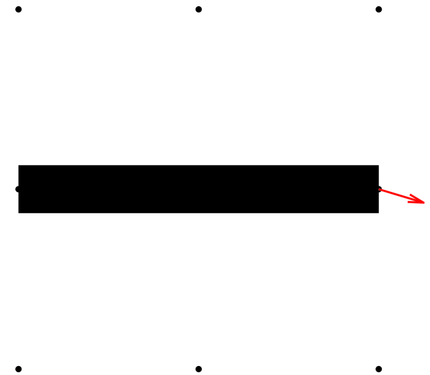
Figure 2: Example 1: ground structure, loads and boundary conditions (left) and the optimal design, together with the most dangerous perturbation (right).

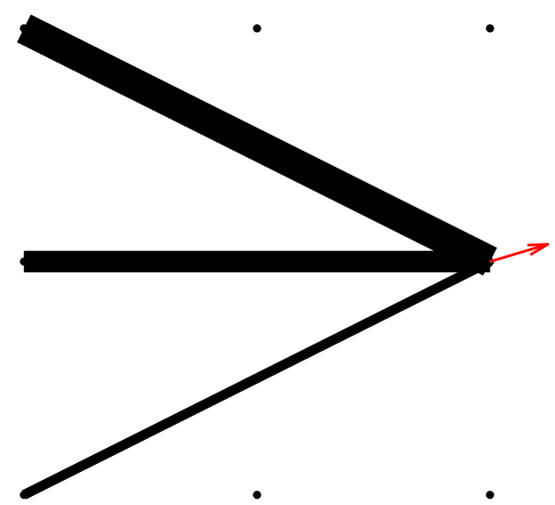
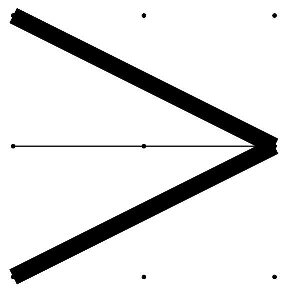
Figure 3: Example 1: Optimal design after the first iteration (left) and robust optimal design (right).

Table 1: Example 1: iteration count “iter”, vulnerability ${\cal V}$, maximal compliance of the current problem “compl”, compliance of the current design with respect to the nominal loads “compl₀, and the worst perturbation for the previous design $f_{s}$.

iter	${\cal V}$	compl	compl0	$f_{s}$
0	Inf	1.0	1.0	[10.0, 0.0]
1	2.25	1.46	1.46	[10.0, 3.0]
2	1.00	1.90	1.38	[10.0, -3.0]

The computed critical perturbation may seem obvious, simply the extreme perturbation of the nominal force “up” and “down”. Again, that is why we have chosen this example, in order to show that the results obtained by the algorithm correspond the engineering intuition.

Example 2

We now consider a higher dimensional example of a long slender truss with 55 nodes and 1485 potential bars. This is again a single-load problem with a single horizontal force applied at the middle right-hand side node. The optimal results of the nominal problem and of the robust problem are shown in Fig. 4 left and right, respectively.

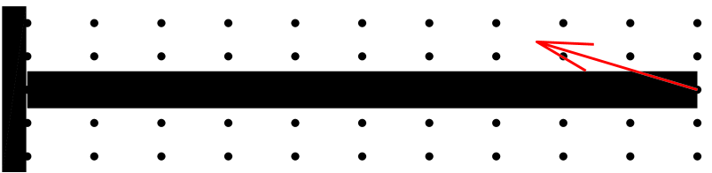
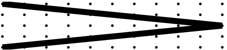
Figure 4: Example 2: optimal design for the nominal load, together with the most dangerous perturbation (left) and robust optimal design (right).

The following Table 2 shows that we only needed two iterations of Algorithm 1 to obtain a robust solution.

Table 2: Example 2, same description as in Table 1

iter	${\cal V}$	compl	compl0	$f_{s}$
0	Inf	10.0	10.0	[10.0, 0.0]
1	3.86	90.17	64.68	[10.0, 3.0]
2	1.00	101.50	10.15	[10.0, -3.0]

Example 3

Let us now solve a problem with three load cases, each on them represented by a single force, as shown in Fig. 5-left. The ground structure consists of 25 nodes and 300 potential bars. Fig. 5-right shows the optimal structure for the nominal loads, as well as the most dangerous perturbations of the nominal loads for this structure. Due to the “free” bar in the top part, this structure is extremely unstable with respect to perturbations and its vulnerability tends to infinity, as shown in Table 3. After the first iteration of Algorithm 1, we obtain the truss shown in Fig. 6-left. This truss is still not robust enough with respect to the depicted load perturbations and its vulnerability is ${\cal V}=1.55$. Finally, after the second iteration of Algorithm 1, we obtain the optimal structure shown in Fig. 6-right. This truss is robust with respect to allowed perturbations.

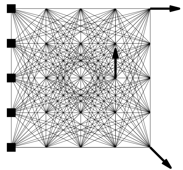
Figure 5: Example 3: ground structure, loads and boundary conditions (left) and the optimal design, together with the most dangerous perturbation (right).

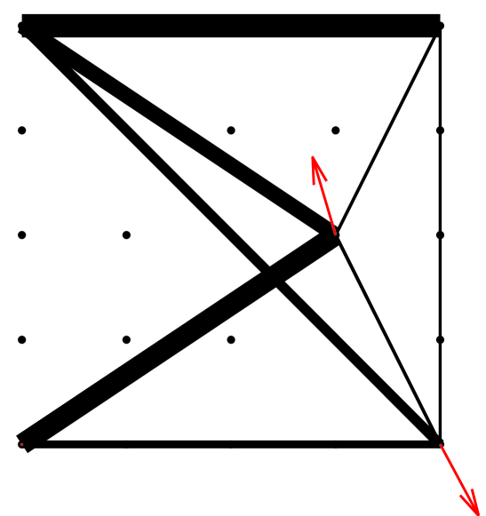
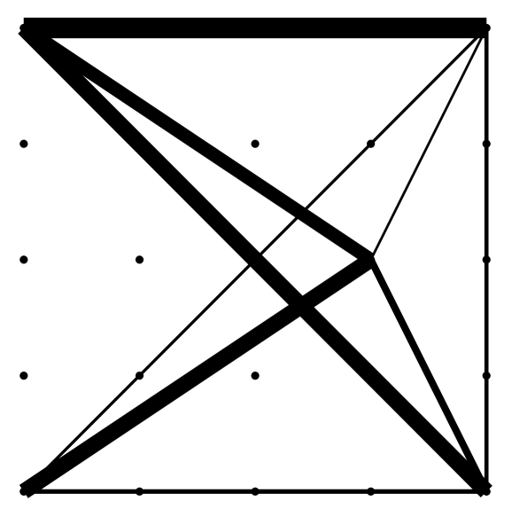
Figure 6: Example 3: Optimal design after the first iteration (left) and robust optimal design (right).

Table 3: Example 3, same description as in Table 1

iter	${\cal V}$	compl	compl0	$f_{s}$
0	Inf	4.82	4.82	[10, 0]; [0, 10]; [7, -7]
1	1.55	6.08	6.08	[10, -2.97]; [2.97, 10]; [9.1, -4.9]
2	1.00	6.61	6.30	N/A; [-2.97, 10]; [4.9, -9.1]

4.2 Variable thickness sheet

In the variable thickness sheet (or free sizing) problem, we consider plane strain linear elasticity model discretized by the standard finite element method. The design variables $x_{i}$ are the thicknesses of the plate, which are assumed to be constant on each finite element; so we have as many variables as elements. Again, the model can be found, e.g. in Bendsøe and Sigmund (2002).

To make the results more transparent, we consider a material with zero Poisson ratio.

Example 4

Consider a rectangular plate as depicted in Fig. 7-left. The plate is fixed on its left-hand side (by prescribed homogeneous boundary conditions at the corresponding nodes) and subject to a horizontal load applied to a small segment in the middle of the right-hand side edge. Fig. 7-right shows the optimal result of this single load problem—a single horizontal bar (recall that the result is due to the zero Poisson ratio). The first line in Table 4 shows that this design is far from being robust; its vulnerability is almost 36. In the same table, in the second row, we can see the critical perturbation of the three prescribed forces. If we add these forces as a load number two and solve the corresponding two-load problem, we obtain an optimal solution depicted in Fig. 8-left. This solution is still not robust; its vulnerability is ${\cal V}=3.35$. But after another iteration of Algorithm 1, we obtain a robust design shown in Fig. 8-right.

Figure 7: Example 4: computational domain, loads and boundary conditions (left) and the optimal design, together with the most dangerous perturbation (right).

Figure 8: Example 4: Optimal design after the first iteration (left) and robust optimal design (right).

Table 4: Example 4, same description as in Table 1

iter	${\cal V}$	compl	compl0	$f_{s}$
0	35.93	48.88	48.88	[1, 0, 2, 0, 1, 0]
1	3.35	78.28	78.28	[1, 0.25, 2, 0.41, 1, 0.56]
2	1.04	111.80	56.54	[1, -0.42, 2, -0.42, 1, -0.43]

References

- Ben-Tal and Nemirovski (1997) Ben-Tal A, Nemirovski A (1997) Robust truss topology design via semidefinite programming. SIAM Journal on Optimization 7(4):991–1016
- Ben-Tal and Nemirovski (2001) Ben-Tal A, Nemirovski A (2001) Lectures on Modern Convex Optimization. MPS-SIAM Series on Optimization. SIAM Philadelphia
- Ben-Tal et al (2009) Ben-Tal A, El Ghaoui L, Nemirovski A (2009) Robust optimization. Princeton University Press
- Bendsøe and Sigmund (2002) Bendsøe M, Sigmund O (2002) Topology Optimization. Theory, Methods and Applications. Springer-Verlag, Heidelberg
- Conti et al (2009) Conti S, Held H, Pach M, Rumpf M, Schultz R (2009) Shape optimization under uncertainty-a stochastic programming perspective. SIAM Journal on Optimization 19(4):1610–1632
- Doltsinis and Kang (2004) Doltsinis I, Kang Z (2004) Robust design of structures using optimization methods. Computer Methods in Applied Mechanics and Engineering 193(23):2221–2237
- El Ghaoui and Lebret (1997) El Ghaoui L, Lebret H (1997) Robust solutions to least-squares problems with uncertain data. SIAM Journal on Matrix Analysis and Applications 18(4):1035–1064
- Evgrafov et al (2003) Evgrafov A, Patriksson M, Petersson J (2003) Stochastic structural topology optimization: existence of solutions and sensitivity analyses. ZAMM-Journal of Applied Mathematics and Mechanics/Zeitschrift für Angewandte Mathematik und Mechanik 83(7):479–492
- Fiala et al (2013) Fiala J, Kočvara M, Stingl M (2013) PENLAB: A MATLAB solver for nonlinear semidefinite optimization. Mathematical Programming Computation Submitted
- Kočvara et al (2000) Kočvara M, Zowe J, Nemirovski A (2000) Cascading—an approach to robust material optimization. Computers & Structures 76:431–442
- Mattheij and Söderlind (1987) Mattheij RM, Söderlind G (1987) On inhomogeneous eigenvalue problems. Linear Algebra and its Applications 88:507–531