Relations Between Stochastic Orderings and generalized Stochastic Precedence

Abstract.

The concept of stochastic precedence between two real-valued random variables has often emerged in different applied frameworks. In this paper we consider a slightly more general, and completely natural, concept of stochastic precedence and analyze its relations with the notions of stochastic ordering. Such a study leads us to introducing some special classes of bivariate copulas. Motivations for our study can arise from different fields. In particular we consider the frame of Target-Based Approach in decisions under risk. This approach has been mainly developed under the assumption of stochastic independence between “Prospects” and “Targets”. Our analysis concerns the case of stochastic dependence.

Keywords. Target Based Utilities, Decision Analysis, Non-Symmetric Copulas, Times to Words’ Occurrences.

1. Introduction.

Let $X_{1},X_{2}$ be two real random variables defined on a same probability space $(\Omega,\mathcal{F},\mathbb{P})$. We will denote by $F$ the joint distribution function and by $G_{1}$, $G_{2}$ their marginal distribution functions, respectively. For the sake of notational simplicity, we will initially concentrate our attention on the case when $G_{1},G_{2}$ belong to the class $\mathcal{G}$ of all the probability distribution functions on the real line, that are continuous and strictly increasing in the domain where they are positive and smaller than one. As we shall see later, we can also consider more general cases, but the present restriction allows us to simplify the formulation and the proofs of our results. In order to account for some cases of interest with $\mathbb{P}(X_{1}=X_{2})>0$, we will not assume that the distribution function $F$ is absolutely continuous.

The random variable $X_{1}$ is said to stochastically precede $X_{2}$ if $\mathbb{P}(X_{1}\leq X_{2})\geq 1/2$, written $X_{1}\preceq_{sp}X_{2}$. The interest of this concept for applications has been pointed out several times in the literature (see in particular [1], [3] and [9]). We recall the reader’s attention on the fact that stochastic precedence does not define a stochastic order in that, for instance, it is not transitive. However it can be considered in some cases as an interesting condition, possibly alternative to the usual stochastic ordering $X_{1}\preceq_{st}X_{2}$, defined by the inequality $G_{1}(t)\geq G_{2}(t),\,\forall t\in\mathbb{R}$, see [14].

When $X_{1},X_{2}$ are independent the implication $X_{1}\preceq_{st}X_{2}\Rightarrow X_{1}\preceq_{sp}X_{2}$ holds (see [1]). It is also easy to find several other examples of bivariate probability models where the same implication holds. For instance the condition $X_{1}\preceq_{st}X_{2}$ even entails $\mathbb{P}(X_{1}\leq X_{2})=1$ when $X_{1},X_{2}$ are comonotonic (see e.g. [11]), i.e. when ${\mathbb{P}}(X_{2}=G_{2}^{-1}(G_{1}(X_{1})))$. On the other hand, cases of stochastic dependence can be found where the implication $X_{1}\preceq_{st}X_{2}\Rightarrow X_{1}\preceq_{sp}X_{2}$ fails. A couple of examples will be presented in Section 3. See also Proposition 7. On the other hand the frame of words’ occurrences produces, in a natural way, examples in the same direction, see e.g. [6].

In this paper we replace the notion $X_{1}\preceq_{sp}X_{2}$ with the generalized concept defined as follows

Definition 1.

For given $\gamma\in[0,1]$, we say that $X_{1}$ stochastically precedes $X_{2}$ at level $\gamma$ if $\mathbb{P}(X_{1}\leq X_{2})\geq\gamma$. This will be written $X_{1}\preceq_{sp}^{(\gamma)}X_{2}$.

Let $\mathcal{C}$ denote the class of all bivariate copulas (see e.g. [7, 11]). Several arguments along the paper, we be based on the concept of bivariate copula and the class of all bivariate copulas will be denoted by $\mathcal{C}$. We say that the pair of random variables $X_{1},X_{2}$, with distributions $G_{1},G_{2}$, respectively, admits $C\in\mathcal{C}$ as its connecting copula whenever its joint distribution function is given by

$$F(x_{1},x_{2})=C(G_{1}(x_{1}),G_{2}(x_{2})).$$ (1)

It is well known (see e.g. [11]) that the connecting copula is unique when $G_{1}$ and $G_{2}$ are continuous. We will use the notation

$$A:=\{(x_{1},x_{2})\in\mathbb{R}^{2}\,:\,x_{1}\leq x_{2}\},$$ (2)

so that we write

$${\mathbb{P}}(X_{1}\leq X_{2})=\int_{A}\,dF(x_{1},x_{2})=\int_{\mathbb{R}^{2}}\mathbf{1}_{A}(x_{1},x_{2})\,dF(x_{1},x_{2}).$$ (3)

For given $G_{1},G_{2}\in\mathcal{G}$ and $C\in\mathcal{C}$ we also set

$$\eta(C,G_{1},G_{2}):=\mathbb{P}(X_{1}\leq X_{2}),$$ (4)

where $X_{1}$ and $X_{2}$ are random variables with distributions $G_{1},G_{2}$ respectively, and connecting copula $C$. Thus the condition $X_{1}\preceq_{sp}^{(\gamma)}X_{2}$ can also be written $\eta(C,G_{1},G_{2})\geq\gamma$.

Suppose now that $X_{1},X_{2}$ satisfy the condition $X_{1}\preceq_{st}X_{2}$. As a main purpose of this paper we give a lower bound for the probability $\mathbb{P}(X_{1}\leq X_{2})$ in terms of the stochastic dependence between $X_{1}$ and $X_{2}$ or, more precisely, in terms of conditions on the integral $\int_{A\cap[0,1]^{2}}dC$. More specifically we will analyze different aspects of the special classes of bivariate copulas, defined as follows.

Definition 2.

For $\gamma\in[0,1]$, we denote by $\mathcal{L}_{\gamma}$ the class of all copulas $C\in\mathcal{C}$ such that

$$\eta(C,G_{1},G_{2})\geq\gamma$$ (5)

for all $G_{1},G_{2}\in\mathcal{G}$ with $G_{1}\preceq_{st}G_{2}$.

Concerning the role of the concept of copula in our study, we point out the following simple facts. Consider the random variables $X_{1}^{\prime}=\phi(X_{1})$ and $X_{2}^{\prime}=\phi(X_{2})$ where $\phi:\mathbb{R}\rightarrow\mathbb{R}$ is a strictly increasing function. Thus $X_{1}^{\prime}\preceq_{st}X_{2}^{\prime}$ if and only if $X_{1}\preceq_{st}X_{2}$ and $X_{1}^{\prime}\preceq_{sp}^{(\gamma)}X_{2}^{\prime}$ if and only if $X_{1}\preceq_{sp}^{(\gamma)}X_{2}$. At the same time the pair $X_{1}^{\prime},X_{2}^{\prime}$ also admits the same connecting copula $C$.

The arguments treated in this paper can reveal of interest in the frame of different applied fields. Motivations for this study, in particular, had arisen for us from the following two fields:

• the Target-Based Approach in utility theory;

• comparisons among waiting times to occurrences of words in random sequences of letters from an alphabet.

Further applications can arise e.g. in the fields of reliability and in the comparison of pool obtained by two opposite coalitions.

More precisely the structure of the paper is as follows. In Section 2, we analyze the main aspects of the class $\mathcal{L}_{\gamma}$ and present a related characterization. Some further basic properties will be detailed in Section 3, where a few examples will be also presented. Finally, in Section 4, we will briefly review Target-Based utilities, pointing out the relations with our work, in the case of stochastic dependence between targets and prospects. Connections with the field of times to words’ occurrences will be discussed in a subsequent note.

2. A characterization of the class $\mathcal{L}_{\gamma}$.

This Section will be devoted to providing a characterization of the class $\mathcal{L}_{\gamma}$ (see Theorem 5 and 6) along with related discussions. We start by detailing a few basic properties of the quantities $\eta(C,G_{1},G_{2})$, for $G_{1},G_{2}\in\mathcal{G}$ and $C\in\mathcal{C}$. In view of the condition $G_{1},G_{2}\in\mathcal{G}$ we can use the change of variables $u=G_{1}(x_{1})$, $v=G_{2}(x_{2})$. Thus we can rewrite the integral in (3) according to the following

Proposition 1.

For given $G_{1},G_{2}\in$ $\mathcal{G}$ and $C\in\mathcal{C}$, one has

$$\eta(C,G_{1},G_{2})=\int_{[0,1]^{2}}\mathbf{1}_{A}(G_{1}^{-1}(u),G_{2}^{-1}(v))\,dC(u,v).$$ (6)

The use of the next Proposition is two-fold: it will be useful both for characterizing the class $\mathcal{L}_{\gamma}$ and establishing lower and upper bounds on the quantity $\eta(C,G_{1},G_{2})$.

Proposition 2.

Let $G_{1},G_{1}^{\prime},G_{2},G_{2}^{\prime}\in\mathcal{G}$. Then

$$G_{2}\preceq_{st}G_{2}^{\prime} \Rightarrow\eta(C,G_{1},G_{2})\leq\eta(C,G_{1},G_{2}^{\prime});$$

$$G_{1}\preceq_{st}G_{1}^{\prime} \Rightarrow\eta(C,G_{1},G_{2})\geq\eta(C,G_{1}^{\prime},G_{2}).$$

Proof.

We prove only the first relation of Proposition 2, since the proof for the second one is analogous. By hypothesis, and since $G_{1},G_{2}^{\prime}\in\mathcal{G}$ for each $x\in(0,1)$, one has

$$G_{2}^{-1}(x)\leq G_{2}^{\prime-1}(x).$$

Therefore

$$(G_{1}^{-1}(x),G_{2}^{-1}(x))\in A\Rightarrow(G_{1}^{-1}(x),G_{2}^{\prime-1}(x))\in A\,.$$

Hence, the proof can be concluded by recalling (6). ∎

From Proposition 2, in particular we get

$$\eta(C,G,G)\leq\eta(C,G^{\prime},G)\qquad\mbox{ and }\qquad\eta(C,G,G)\leq\eta(C,G,G^{\prime\prime})\,,$$ (7)

for any choice of $G,G^{\prime},G^{\prime\prime}\in\mathcal{G}$ such that $G^{\prime}\preceq_{st}G\preceq_{st}G^{\prime\prime}$.

A basic fact in the analysis of the classes $\mathcal{L}_{\gamma}$ is that the quantities of the form $\eta(C,G,G)$ only depend on the copula $C$. More formally we state the following result.

Proposition 3.

For any pair of distribution functions $G^{\prime},G^{\prime\prime}\in\mathcal{G}$, one has

$$\eta(C,G^{\prime},G^{\prime})=\eta(C,G^{\prime\prime},G^{\prime\prime})\,,$$ (8)

Proof.

Recalling (6) one obtains

$$\int_{[0,1]^{2}}\mathbf{1}_{A}(G^{\prime-1}(u),G^{\prime-1}(v))\,dC(u,v)=\int_{[0,1]^{2}}\mathbf{1}_{A}(G^{\prime\prime-1}(u),G^{\prime\prime-1}(v))\,dC(u,v)$$ (9)

because $\mathbf{1}_{A}(G^{\prime-1}(u),G^{\prime-1}(v))=\mathbf{1}_{A}(G^{\prime\prime-1}(u),G^{\prime\prime-1}(v))=\mathbf{1}_{A}(u,v)$, so equality in (8) is proved. ∎

As a consequence of Proposition 3 we can introduce the symbol

$$\eta(C):=\eta(C,G,G),$$ (10)

and, by letting $G_{1}=G_{2}=G$ in (6), write

$$\eta(C)=\int_{A\cap[0,1]^{2}}dC$$ (11)

for $G\in\mathcal{G}$. From Proposition 2 and from the inequalities (7), we obtain

Proposition 4.

For $G_{1},G_{2}\in\mathcal{G}$ the following implication holds

$$G_{1}\preceq_{st}G_{2}\Rightarrow\eta(C)\leq\eta(C,G_{1},G_{2}).$$

We then see that the quantity $\eta(C)$ characterizes the class $\mathcal{L}_{\gamma},\,0\leq\gamma\leq 1$, in fact we can state the following

Theorem 5.

$C\in\mathcal{L}_{\gamma}$ if and only if $\,\eta(C)\geq\gamma$.

We thus have

$$\mathcal{L}_{\gamma}=\{C\in\mathcal{C}:\eta(C)\geq\gamma\}$$ (12)

and we can also write

$$\eta(C)=\inf_{G_{1},G_{2}\in\mathcal{G}}\{\eta(C,G_{1},G_{2}):G_{1}\preceq_{st}G_{2}\}.$$ (13)

In other words the infimum in formula (13) is a minimum and it is attained when $G_{1}=G_{2}$. We notice furthermore that the definition of $\eta(C,G_{1},G_{2})$ can be extended to the case when $G_{1},G_{2}\in D(\mathbb{R})$, the space of distribution functions on $\mathbb{R}$. The class $\mathcal{G}$ has however a special role in the present setting, as it is shown in the following result.

Theorem 6.

Let $C\in\mathcal{C}$, $G,H\in D(\mathbb{R})$ with $G\preceq_{st}H$, then $\eta(C,G,H)\geq\eta(C)$.

Proof.

Consider two sequences $(G_{n}:n\in\mathbb{N})$, $(H_{n}:n\in\mathbb{N})$ such that $G_{n},H_{n}\in\mathcal{G}$ and $G_{n}\stackrel{{\scriptstyle w}}{{\to}}G$, $H_{n}\stackrel{{\scriptstyle w}}{{\to}}H$. Applying the Theorem 2 in [13], we obtain that $C(G_{n},H_{n})\stackrel{{\scriptstyle w}}{{\to}}C(G,H)$.

Take the new sequence $(\tilde{H}_{n}:n\in\mathbb{N})$ where $\tilde{H}_{n}(x):=\min\{G_{n}(x),H_{n}(x)\}$. We notice that $\tilde{H}_{n}\in\mathcal{G}$, moreover $G_{n}\preceq_{st}\tilde{H}_{n}$ and $\tilde{H}_{n}\stackrel{{\scriptstyle w}}{{\to}}H$. This implies $C(G_{n},\tilde{H}_{n})\stackrel{{\scriptstyle w}}{{\to}}C(G,H)$.

Now using the standard characterization of weak convergence on separable spaces (see [2] p. 67 Theorem 6.3)

$$\limsup_{n\to\infty}\int_{B}d\tilde{F}_{n}\leq\int_{B}dF\,,$$

for any closed set $B\in\mathbb{R}^{2}$, where $F=C(G,H)$ and $\tilde{F}_{n}=C(G_{n},\tilde{H}_{n})$. Taking the closed set $A$ defined in (2) one has

$$\eta(C)\leq\limsup_{n\to\infty}\int_{A}d\tilde{F}_{n}\leq\int_{A}dF=\eta(C,G,H).$$ (14)

∎

Remark 2.1.

Theorem 6 shows that the minimum of $\eta(C,G,H)$, for $G,H\in D(\mathbb{R})$, is attained at $(C,G,G)$, for any $G\in\mathcal{G}\subset D(\mathbb{R})$. This result allows us to replace the class $\mathcal{G}$ with $D(\mathbb{R})$ in the expression of $\mathcal{L}_{\gamma}$ given in (13). We notice furthermore that one can have $\eta(C,G^{\prime},G^{\prime})\neq\eta(C,G^{\prime\prime},G^{\prime\prime})$ when $G^{\prime},G^{\prime\prime}$ are in $D(\mathbb{R})$.

Concerning the classes $\mathcal{L}_{\gamma}$, we also define

$$\mathcal{B}_{\gamma}:=\{C\in\mathcal{C}\,|\,\eta(C)=\gamma\},$$ (15)

so that

$$\mathcal{L}_{\gamma}=\bigcup_{\gamma^{\prime}\geq\gamma}\mathcal{B}_{\gamma^{\prime}}.$$

We now show that the classes $\mathcal{B}_{\gamma}$, $\gamma\in[0,1]$, are all non empty. Several natural examples might be produced on this purpose. We fix attention on a simple example built in terms of the random variables $X_{1}$, $X_{2}^{(\gamma)}$ defined as follows. On the probability space $([0,1],\mathcal{B}[0,1],\lambda)$, where $\lambda$ denotes the Lebesgue measure, we take $X_{1}(\omega)=\omega$, and

$$X_{2}^{(\gamma)}(\omega)=\left\{\begin{array}[c]{ll}\omega+1-\gamma&\text{ if }\omega\in[0,\gamma],\\ \omega-\gamma&\text{ if }\omega\in(\gamma,1].\end{array}\right.$$ (16)

As it happens for $X_{1}$, also the distribution of $X_{2}^{(\gamma)}$ is uniform in $[0,1]$ for any $\gamma\in[0,1]$ and the connecting copula of $X_{1},X_{2}^{(\gamma)}$, that is then uniquely determined, will be denoted by $C_{\gamma}$.

Proposition 7.

For any $\gamma\in(0,1]$, one has

• $C_{\gamma}\in\mathcal{B}_{\gamma}$.

• $C_{\gamma}(u,v)=\min\{u,v,\max\{u-\gamma,0\}+\max\{v+\gamma-1,0\}\}$.

Proof.

(i) First we notice that ${\mathbb{P}}(X_{1}\leq X_{2}^{(\gamma)})=\gamma$. In fact

$$\mathbb{P}(X_{1}\leq X_{2}^{(\gamma)})={\mathbb{P}}(X_{1}\leq X_{1}+1-\gamma,X_{1}\leq\gamma)+\mathbb{P}(X_{1}\leq X_{1}-\gamma,X_{1}>\gamma)=\gamma.$$

Whence, $\eta(C_{\gamma})=\mathbb{P}(X_{1}\leq X_{2}^{(\gamma)})=\gamma$, since both the distributions of $X_{1},X_{2}^{(\gamma)}$ belong to $\mathcal{G}$.

(ii) For $x_{1},x_{2}\in[0,1]$ we can write

$$F_{X_{1},X_{2}^{(\gamma)}}(x_{1},x_{2}) :=\mathbb{P}(X_{1}\leq x_{1},X_{2}^{(\gamma)}\leq x_{2})$$

$$=\mathbb{P}(X_{1}\leq x_{1},X_{1}+1-\gamma\leq x_{2},\,X_{1}\leq\gamma)$$

$$\,+\mathbb{P}(X_{1}\leq x_{1},X_{1}\leq x_{2}+\gamma,\,X_{1}>\gamma)$$

$$=\mathbb{P}(X_{1}\leq\min\{x_{1},x_{2}+\gamma-1,\gamma\})+\mathbb{P}(\gamma<X_{1}\leq\min\{x_{1},x_{2}+\gamma\})$$

$$=\max\{\min\{x_{1},x_{2}+\gamma-1,\gamma\},0\}+\max\{\min\{x_{1},x_{2}+\gamma\}-\gamma,0\}$$

$$=\min\{x_{1},x_{2},\max\{x_{1}-\gamma,0\}+\max\{x_{2}+\gamma-1,0\}\}\,.$$

Since both the marginal distributions of $X_{1}$ and $X_{2}^{(\gamma)}$ are uniform, it follows that

$$C_{\gamma}(u,v)=\min\{u,v,\max\{u-\gamma,0\}+\max\{v+\gamma-1,0\}\}.$$

∎

The copulas $C_{\gamma}$ have also been considered for different purposes in the literature, see e.g. [12] and [15]. We point out that the identity $\eta(C_{\gamma})=\gamma$ (for $\gamma\in(0,1]$) could also have been obtained directly from formula (11). In this special case the computation of ${\mathbb{P}}(X_{1}\leq X_{2})$ is however straightforward.

As an immediate consequence of Proposition 7 we have that $\mathcal{L}_{\gamma^{\prime}}$ is strictly contained in $\mathcal{L}_{\gamma}$ for any $0\leq\gamma<\gamma^{\prime}\leq 1$. We notice furthermore that $\mathcal{L}_{0}=\mathcal{C}$ and $\mathcal{L}_{1}=\{C\in\mathcal{C}:\int_{A\cap[0,1]^{2}}dC=1\}\neq\emptyset$.

Graphs of $C_{\gamma}$ for different values of $\gamma$ are provided in Figure 1.

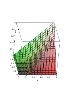
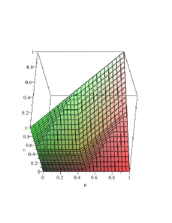
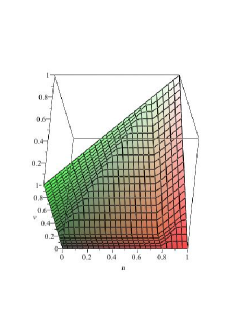
Figure 1. Copulas from the family $C_{\gamma}$ with $\gamma=0.3,\,0.5,\,0.8$ respectively

3. Further properties of $\mathcal{L}_{\gamma}$ and examples

We start this Section by analyzing further properties of the classes $\mathcal{L}_{\gamma}$ that can also shed light on the relations between stochastic precedence and stochastic orderings. First we notice that the previous Definition 2 has been formulated in terms of the usual stochastic ordering $\preceq_{st}$. However similar results can also be obtained for other important concepts of stochastic ordering that have been considered in the literature (such as the hazard rate, the likelihood ratio, and the mean residual life orderings, see [14]).

Let us fix, in fact, a stochastic ordering $\preceq_{\ast}$ different from $\preceq_{st}$. Definition 2 can be modified by replacing therein $\preceq_{st}$ with $\preceq_{\ast}$ and this operation leads us to a new class of copulas that we can denote by $\mathcal{L}_{\gamma}^{(\ast)}$. More precisely we set

$$\mathcal{L}^{(*)}_{\gamma}:=\{C\in\mathcal{C}:\eta(C,G_{1},G_{2})\geq\gamma,\;\forall\,G_{1},G_{2}\in\mathcal{G}\;s.t.\;G_{1}\preceq_{*}G_{2}\}$$ (17)

or equivalently

$$\mathcal{L}^{(*)}_{\gamma}=\{C\in\mathcal{C}:\eta^{*}(C)\geq\gamma\}$$ (18)

where

$$\eta^{*}(C):=\inf_{G_{1},G_{2}\in\mathcal{G}}\{\eta(C,G_{1},G_{2}):G_{1}\preceq_{\ast}G_{2}\}.$$ (19)

For given $\gamma\in(0,1)$, one might wonder about possible relations between $\mathcal{L}_{\gamma}^{(\ast)}$ and $\mathcal{L}_{\gamma}$. Actually one has the following result, which will be formulated for binary relations (not necessarily stochastic orderings) over the space $D({\mathbb{R}})$.

Proposition 8.

Let $\preceq_{\ast}$ be a relation satisfying

• for any $G\in D(\mathbb{R})$ one has $G\preceq_{\ast}G$;

• for any $G_{1},G_{2}\in D(\mathbb{R})$ with $G_{1}\preceq_{\ast}G_{2}$ one has $G_{1}\preceq_{st}G_{2}$.

Then $\mathcal{L}_{\gamma}=\mathcal{L}_{\gamma}^{(\ast)}$.

Proof.

In view of (b), one has that $\eta(C)\leq\eta^{*}(C)$. In fact both the quantities $\eta(C)$ and $\eta^{*}(C)$ are obtained as an infimum of the same functional and, compared with $\eta$, the quantity $\eta^{*}$ is an infimum computed on a smaller set.

Due to (a), however, $\eta(C)$ and $\eta^{*}(C)$ are both obtained, in (13) and (19) respectively, as minima attained on a same point $(G,G)$. We can then conclude that $\mathcal{L}^{(*)}_{\gamma}=\mathcal{L}_{\gamma}$. ∎

Concerning Proposition 8 we notice that, for example, the hazard rate and the likelihood ratio orderings, $\preceq_{hr}$ and $\preceq_{lr}$, both satisfy the conditions (a) and (b).

In applied problems it can be relevant to remark that imposing stochastic orderings stronger than $\preceq_{st}$ does not necessarily increase the level of stochastic precedence.

For the sake of notational simplicity we come back to considering the usual stochastic ordering $\preceq_{st}$ and the class $\mathcal{L}_{\gamma}$.

For what follows it is now convenient also to consider the quantities $\xi(C,G_{1},G_{2})$ and $\xi(C)$ defined as follows:

$$\xi(C,G_{1},G_{2}) :=\mathbb{P}(X_{1}=X_{2}),$$ (20)

$$\xi(C) :=\xi(C,G,G),$$ (21)

where $X_{1}$ and $X_{2}$ are random variables with distributions $G_{1},G_{2}\in\mathcal{G}$ respectively and connecting copula $C$.

For a given bivariate model we have considered so far the quantities $\eta(C)$ with $C$ denoting the connecting copula. In what follows we point out the relations among $\eta(C)$, $\eta(\widehat{C})$, $\eta(C^{t})$ where $\widehat{C}$ and $C^{t}$ denote the survival copula and the transposed copula, respectively. The transposed copula $C^{t}$ is defined by

$$C^{t}(u,v):=C(v,u)$$ (22)

so that if $C$ is the connecting copula of the pair $(X_{1},X_{2})$, then $C^{t}$ is the copula of the pair $(X_{2},X_{1})$. Whence, if $X_{1}$ and $X_{2}$ have the same distribution $G\in\mathcal{G}$, then

$$\eta(C^{t})={\mathbb{P}}(X_{2}\leq X_{1}).$$

On the other hand the notion of survival copula of the pair $(X_{1},X_{2})$, which comes out as natural when considering pairs of non-negative random variables, is defined by the equation

$$\overline{F}_{X_{1},X_{2}}(x_{1},x_{2})=\widehat{C}\left[\overline{G}_{1}(x_{1}),\overline{G}_{2}(x_{2})\right],$$ (23)

with $\overline{G}_{1}$ and $\overline{G}_{2}$ respectively denoting the marginal survival functions:

$$\overline{G}_{1}(x_{1})=\mathbb{P}(X_{1}>x_{1}),\quad\overline{G}_{2}(x_{2})=\mathbb{P}(X_{2}>x_{2})\,.$$

The relationship between the survival copula $\widehat{C}$ of $(X_{1},X_{2})$ and the connecting copula $C$ is given by (see [11])

$$\widehat{C}(u,v)=u+v-1+C(1-u,1-v).$$ (24)

The following result shows the relations tying the different quantities $\eta(C)$, $\eta(\widehat{C})$, $\eta(C^{t})$. The proof is easy and will be omitted.

Proposition 9.

Let $C\in\mathcal{C}$. The following relation holds:

$$\eta(\widehat{C})=\eta(C^{t})=1-\eta(C)+\xi(C).$$

A basic property of the classes $\mathcal{L}_{\gamma}$ and $\mathcal{B}_{\gamma}$ is given by the following result.

Proposition 10.

For $\gamma\in[0,1]$, the classes $\mathcal{L}_{\gamma}$, $\mathcal{L}_{\gamma}^{c}=\mathcal{C}\setminus\mathcal{L}_{\gamma}$, and $\mathcal{B}_{\gamma}$ are convex.

Proof.

We consider two bivariate copulas $C_{1},C_{2}\in\mathcal{L}_{\gamma}$ and a convex combination of them, i.e. take $\alpha\in(0,1)$ and $C:=\alpha C_{1}+(1-\alpha)C_{2}$. We show that $C\in\mathcal{L}_{\gamma}$, indeed

$$\eta(C)=\int_{A}dC(u,v)=\alpha\int_{A}dC_{1}(u,v)+(1-\alpha)\int_{A}dC_{2}(u,v)=\alpha\eta(C_{1})+(1-\alpha)\eta(C_{2}).$$

Since $\eta(C_{1}),\eta(C_{2})$ are larger or equal than $\gamma$ then $\eta(C)\geq\gamma$, whence $\mathcal{L}_{\gamma}$ is convex. Now one can use the same argument in order to show that $\mathcal{L}_{\gamma}^{c}$ and $\mathcal{B}_{\gamma}$ are convex as well. ∎

An immediate application of Proposition 10 concerns the case when, given a random parameter $\Theta$, all the connecting copulas of the conditional distributions of $(T,X)$, belong to a same class $\mathcal{L}_{\gamma}$. Proposition 10 in fact, guarantees that the copula of $(T,X)$ belongs to $\mathcal{L}_{\gamma}$ as well.

Some aspects of the definitions and results given so far will be demonstrated here by presenting a few examples. We notice that, as shown by Proposition 7, the condition $\preceq_{st}$ does not imply $\preceq_{sp}^{(\gamma)}$, with $\gamma\in(0,1)$. For the special case $\gamma=1/2$ we now present an example of applied interest.

Example 1.

Let $X,Y$ be two non-negative random variables, where $Y$ has an exponentially density $f_{Y}(y)$ with failure rate $\lambda$ and where stochastic dependence between $X$ and $Y$ is described by a “load-sharing” dynamic model as follows: conditionally on $(Y=y)$, the failure rate of $X$ amounts to $\alpha=1$ for $t<y$ and to $\beta$ for $t>y$. We assume $1<\lambda<\beta<1+\lambda$. This position gives rise to a jointly absolutely continuous distribution for which we can consider

$$\mathbb{P}(X>x|Y=y):=\int_{x}^{+\infty}f_{X,Y}(t,y)dt,$$

$f_{X,Y}$ denoting the joint density of $X,Y$. As to the survival function of $X$, for any fixed value $x>0$, we can argue as follows.

$$\overline{F}_{X}(x) :=\mathbb{P}(X>x)=\int_{0}^{+\infty}\mathbb{P}(X>x|Y=y)f_{Y}(y)dy$$

$$=\int_{0}^{x}\mathbb{P}(X>x|Y=y)f_{Y}(y)dy+\int_{x}^{+\infty}\mathbb{P}(X>x|Y=y)f_{Y}(y)dy$$

$$=\int_{0}^{x}\mathbb{P}(X>y|Y=y)\mathbb{P}(X>x|Y=y,X>y)f_{Y}(y)dy+\int_{x}^{+\infty}e^{-x}f_{Y}(y)dy$$

$$=\left(1-\frac{\lambda}{1+\lambda-\beta}\right)e^{-(1+\lambda)x}+\frac{\lambda}{1+\lambda-\beta}\,e^{-\beta x}\leq e^{-\lambda x},\quad\forall x>0.$$

We can then conclude that $X\preceq_{st}Y$. On the other hand the same position gives also rise to $\mathbb{P}(X\leq Y)=1/(1+\lambda)<1/2$.

The next example shows that for three random variables $T,X^{\prime},X^{\prime\prime}$, the implication $T\preceq_{st}X^{\prime}\preceq_{st}X^{\prime\prime}\Rightarrow\mathbb{P}(T\leq X^{\prime\prime})\leq\mathbb{P}(T\leq X^{\prime})$ can fail when the connecting copulas of $(T,X^{\prime})$ and $(T,X^{\prime\prime})$ are different.

Example 2.

Let $Y_{1},\ldots,Y_{5}$ be i.i.d. random variables, with a continuous distribution and defined on a same probability space, and set

$$T=\min(Y_{1},Y_{2}),\;X^{\prime}=\max(Y_{1},Y_{2}),\;X^{\prime\prime}=\max(Y_{3},Y_{4},Y_{5}).$$

Thus $X^{\prime}\preceq_{st}X^{\prime\prime}$, but $\mathbb{P}(T\leq X^{\prime})=1$ and $\mathbb{P}(T\leq X^{\prime\prime})<1$.

Remark 3.1.

For some special types of copula $C$, the computation of $\eta(C,G_{1},G_{2})$ can be carried out directly, in terms of probabilistic arguments, provided the distributions $G_{1},G_{2}$ belong to some appropriate class. This circumstance in particular manifests for the models considered in the subsequent examples. Let $C$ be a copula satisfying such conditions. Then Proposition 2 can be used to obtain inequalities for $\eta(C,H_{1},H_{2})$ even if $H_{1},H_{2}$ do not belong to $\mathcal{G}$ provided, e.g., that $H_{1}\preceq_{st}G_{1}$, $G_{2}\preceq_{st}H_{2}$ and $G_{1},G_{2}\in\mathcal{G}$.

The next example will be devoted to bivariate gaussian models, i.e. to a relevant case of symmetric copulas.

Example 3.

Gaussian Copulas.

The family of bivariate gaussian copulas (see e.g. [11]) is parameterized by the correlation coefficient $\rho\in(-1,1)$. The corresponding copula $C^{(\rho)}$ is absolutely continuous and symmetric, and $\eta(C^{(\rho)})=1/2$ and, thus, it does not depend on $\rho$. For fixed pairs of distributions $G_{1},G_{2}$, on the contrary, the quantity $\eta(C^{(\rho)},G_{1},G_{2})$ does actually depend on $\rho$, besides on $G_{1}$ and $G_{2}$. This class provides the most direct instance of the situation outlined in the above Remark 3.1. The value for $\eta(C^{(\rho)},G_{1},G_{2})$ is in fact immediately obtained when $G_{1},G_{2}$ are gaussian. Let $X_{1},X_{2}$ denote gaussian random variables with connecting copula $C^{(\rho)}$ and parameters $\mu_{1},\mu_{2},\sigma_{1}^{2},\sigma_{2}^{2}$. Since the random variable $Z=X_{1}-X_{2}$ is distributed according to $\mathcal{N}(\mu_{1}-\mu_{2},\sigma^{2}_{1}+\sigma^{2}_{2}-2\rho\sigma_{1}\sigma_{2})$ we can write

$$\eta(C^{(\rho)},G_{1},G_{2})={\mathbb{P}}(Z\leq 0)=\Phi\left(\frac{\mu_{2}-\mu_{1}}{\sqrt{\sigma^{2}_{1}+\sigma^{2}_{2}-2\rho\sigma_{1}\sigma_{2}}}\right).$$ (25)

We recall that, when $X_{i}\sim\mathcal{N}(\mu_{i},\sigma_{i}^{2})$ for $i=1,2$, the necessary and sufficient condition for $X_{1}\preceq_{st}X_{2}$ is $\mu_{1}\leq\mu_{2}$ and $\sigma_{1}=\sigma_{2}$ (see e.g. [1]). In other words, for $G_{1},G_{2}$ gaussian, $G_{1}\preceq_{st}G_{2}$ means $X_{1}\preceq_{sp}X_{2}$ and $\sigma_{1}=\sigma_{2}$. By using the formula in (25), with $\sigma_{1}=\sigma_{2}=\sigma$, we have

$$\eta(C^{(\rho)},G_{1},G_{2})=\Phi\left(\frac{\mu_{2}-\mu_{1}}{\sigma\sqrt{2(1-\rho)}}\right).$$ (26)

Thus $G_{1}\preceq_{st}G_{2}\Rightarrow\eta(C^{(\rho)},G_{1},G_{2})\geq 1/2$, as shown by Proposition 4 and Theorem 6. We notice that $\eta(C^{(\rho)},G_{1},G_{2})$ is an increasing function of $\rho$.

Proposition 2 can be extended to obtain, say, that

$$\eta(C^{(\rho)},G_{1},G_{2})\leq\eta(C^{(\rho)},H_{1},H_{2}),$$

when $H_{1}\preceq_{st}G_{1}$ and $G_{2}\preceq_{st}H_{2}$, for $G_{1},G_{2}\in\mathcal{G}$ and $H_{1},H_{2}\notin\mathcal{G}$. We then can give inequalities for $\eta(C^{(\rho)},H_{1},H_{2})$ in terms of (25), provided $H_{1},H_{2}$ are suitably comparable in the $\preceq_{st}$ sense with gaussian distributions.

In the cases when $\xi(C)>0$, we should obviously distinguish between computations of $\mathbb{P}(X_{1}\leq X_{2})$ and $\mathbb{P}(X_{1}<X_{2})$, where $C$ is the connecting copula of $X_{1},X_{2}$. A remarkable case when this circumstance happens is considered in the following example.

Example 4.

Marshall-Olkin Models

We consider the Marshall-Olkin copulas (see e.g [7, 8, 11]), namely those whose expression is the following:

$$\widehat{C}^{(\alpha_{1},\alpha_{2})}(u,v):=u\,v\,\min\{u^{-\alpha_{1}},\,v^{-\alpha_{2}}\}$$

for $0<\alpha_{i}<1$, $i=1,2$. We notice that the Marshall-Olkin copula has a singular part that is concentrated on the curve $u^{\alpha_{1}}=v^{\alpha_{2}}$ (see also Figure 2). Actually the measure of such a singular component is given by

$$\frac{\alpha_{1}\alpha_{2}}{\alpha_{1}+\alpha_{2}-\alpha_{1}\alpha_{2}}.$$

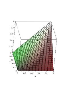
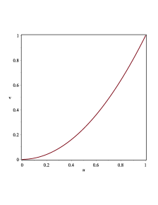
Figure 2. Marshall-Olkin Copula (left) and graph of $u^{\alpha_{1}}=v^{\alpha_{2}}$ (right). Special case $\alpha_{1}=0.4,\,\alpha_{2}=0.2$.

As for the computation of $\eta(\widehat{C}^{(\alpha_{1},\alpha_{2})})$ we use the expression in (11). By separately considering the curve $u^{\alpha_{1}}=v^{\alpha_{2}}$ and the domains where $\widehat{C}^{(\alpha_{1},\alpha_{2})}$ is absolutely continuous, we obtain

$$\eta(\widehat{C}^{(\alpha_{1},\alpha_{2})})=\frac{1}{2-\alpha_{1}\wedge\alpha_{2}}\left(1-\frac{(\alpha_{1}-\alpha_{1}\wedge\alpha_{2})(\alpha_{1}\wedge\alpha_{2})}{\alpha_{1}-\alpha_{2}}\right).$$

Consider the copula

$$C^{(\alpha_{1},\alpha_{2})}(u,v):=\widehat{C}^{(\alpha_{1},\alpha_{2})}(1-u,1-v)+u+v-1.$$

We will see now that the value of $\eta(C^{(\alpha_{1},\alpha_{2})},G_{1},G_{2})$ directly follows from probabilistic arguments, provided $G_{1},G_{2}$ are exponential distributions with appropriate parameters. Let in fact $V$, $W$ and $Z$ be three random variables independent and exponentially distributed with parameters $\mu_{1}=1/\alpha_{1}-1$, $\mu_{2}=1/\alpha_{2}-1$ and $\mu=1$, respectively. The new random variables

$$X_{1}:=V\wedge Z,\qquad X_{2}:=W\wedge Z,$$

have survival copula $\widehat{C}^{(\alpha_{1},\alpha_{2})}$, connecting copula $C^{(\alpha_{1},\alpha_{2})}$, and exponential distributions $G_{1}^{(\alpha_{1})}$ and $G_{2}^{(\alpha_{2})}$, with parameters $1/\alpha_{1}$ and $1/\alpha_{2}$ respectively. We now proceed with the computation of

$$\eta(C^{(\alpha_{1},\alpha_{2})},G_{1}^{(\alpha_{1})},G_{2}^{(\alpha_{2})})={\mathbb{P}}(X_{1}\leq X_{2}).$$

We can write

$$\xi(C^{(\alpha_{1},\alpha_{2})},G_{1}^{(\alpha_{1})},G_{2}^{(\alpha_{2})}) ={\mathbb{P}}(X_{1}=X_{2})={\mathbb{P}}(Z\leq V\wedge W)$$

$$=\frac{1}{\mu_{1}+\mu_{2}+1}=\frac{\alpha_{1}\alpha_{2}}{\alpha_{1}+\alpha_{2}-\alpha_{1}\alpha_{2}},$$

furthermore

$${\mathbb{P}}(X_{1}<X_{2})={\mathbb{P}}(V<W\wedge Z)=\frac{(1-\alpha_{1})\,\alpha_{2}}{\alpha_{1}+\alpha_{2}-\alpha_{1}\alpha_{2}},$$

and finally we obtain

$${\mathbb{P}}(X_{1}\leq X_{2})=\frac{\alpha_{2}}{\alpha_{1}+\alpha_{2}-\alpha_{1}\alpha_{2}}.$$

Then

$$\eta(C^{(\alpha_{1},\alpha_{2})},G_{1}^{(\alpha_{1})},G_{2}^{(\alpha_{2})})=\frac{\alpha_{2}}{\alpha_{1}+\alpha_{2}-\alpha_{1}\alpha_{2}}.$$

We now conclude this Section with an example showing an extreme case in the direction of Remark 3.1.

Example 5.

Copulas of order statistics.

Let $A,B$ be two i.i.d. random variables with distribution function $G\in\mathcal{G}$ and denote by $X_{1},X_{2}$ their order statistics, namely $X_{1}=\min\{A,B\},X_{2}=\max\{A,B\}$. The distributions of $X_{1},X_{2}$ depend on $G$ and are respectively given by

$$F_{1}^{(G)}(x_{1}) ={\mathbb{P}}(\min\{X_{1},X_{2}\}\leq x_{1})=2G(x_{1})-G(x_{1})^{2},$$

$$F_{2}^{(G)}(x_{2}) ={\mathbb{P}}(\max\{X_{1},X_{2}\}\leq x_{2})=G(x_{2})^{2}\,.$$

The connecting copula of $(X_{1},X_{2})$, represented in Figure 3, is given by

$$K(u,v)=\left\{\begin{array}[]{ll}\displaystyle{2(1-(1-u)^{1/2})v^{1/2}-(1-(1-u)^{1/2})^{2}}&\mbox{ if }v\geq(1-(1-u)^{1/2})^{2},\\ \displaystyle{v}&\mbox{ otherwise}.\end{array}\right.$$

We have, by definition,

$$\eta(K,F_{1}^{(G)},F_{2}^{(G)})=1,$$

and it does not depend on $G$. We notice, on the other hand, that the computation of $\eta(K)=\eta(K,G,G)$, with $G\in\mathcal{G}$, is to be carried out explicitly, since the pair $(G,G)$ can never appear as the pair of marginal distributions of order statistics. By recalling (6) one obtains

$$\eta(K)=\int_{[0,1]^{2}}\frac{\mathbf{1}_{A}(u,v)}{2\sqrt{v}\sqrt{1-u}}\,dv\,du=2-\frac{\pi}{2}<\frac{1}{2}.$$

We can extend this example to the case when the connecting copula of $A,B$ is a copula $D$ different from the product copula $\Pi$, but still $A$ and $B$ are identically distributed according to a distribution function $G$. In this case the connecting copula $K$ of $X_{1},X_{2}$ depends on $D$, but again it does not depend on $G$ (see [10] page 478).

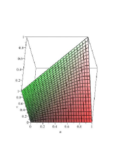
Figure 3. Ordered Statistic Copula K

4. The Target-Based Approach to decisions under risk and the classes $\mathcal{L}_{\gamma}$.

In this Section we will look at the arguments of the previous Sections in the perspective of one-attribute decisions problems under risk and, more in particular, of the related Target-Based Approach (TBA). In such problems, a risky prospect (or lottery) $X$ is nothing else than a real random variable representing, say, the random amount of wealth obtained as the consequence of an action or of an economic investment. An investor (or decision-maker) $I$ is supposed to choose one out of many different actions by evaluating and comparing the different probability distributions corresponding to any single prospect. This choice is implemented on the basis of $I$’s attitudes toward risk.

As very well-known, in such a frame, the Expected Utility Principle first suggests that $I$ describe her/his own attitudes by means of a utility function $U$ ($U:\mathbb{R}\rightarrow\mathbb{R}$) and consequently prescribes that any prospect $X$ (with its probability distribution $F_{X}$) be evaluated in terms of the expected-utility

$$\mathbb{E}(U(X))=\int_{\mathbb{R}}U(x)F_{X}(dx).$$

In the same frame, the Target-Based Approach is based on a different principle. The TBA assumes in fact that the exclusive interest of the investor $I$, in the use of the amount of wealth $X$, is concentrated on the possibility of “buying” a specific good (a house, a car, a block of shares of a stock, etc.). The price of such good is a random variable $T$ (the target), with a probability distribution $F_{T}$. Whence $I$ is for first supposed to specify the target $T$ as a way to describe his/her own attitude with respect to risk. Then $I$ will evaluate any single prospect $X$ in terms of the probability ${\mathbb{P}}(T\leq X)$. The best prospect will be the one that maximizes ${\mathbb{P}}(T\leq X)$. Such an approach was proposed by Bordley, Li Calzi, and Castagnoli (see [4, 5]). Some related ideas were already around in the economic literature in the past and other interesting developments appeared in the subsequent years, especially for what concerns the multi-attribute setting. Generally $T$ and $X$ may in fact also be vectors.

Here we concentrate attention on the single-attribute case where $(T,X)$ are pairs of real-valued random variables. It is clear then that the objects of central interest in the TBA are, for a fixed target $T$, the probabilities $\mathbb{P}(T\leq X)$ and the analysis developed in the previous sections can reveal of interest. We assume the existence of regular conditional distributions. In particular we assume that, for any prospect $X$, we can determine $\upsilon_{T}^{(X)}(x):=\mathbb{P}(T\leq x|X=x)$, so that we can write

$$\mathbb{P}(T\leq X)=\int_{\mathbb{R}}\upsilon_{T}^{(X)}(x)\,dF_{X}(x).$$

Before continuing it is useful to look at the special case when $X$ and $T$ are stochastically independent. We can thus write

$$\mathbb{P}(T\leq X) =\int_{\mathbb{R}}\upsilon_{T}^{(X)}(x)\,dF_{X}(x)=\int_{\mathbb{R}}F_{T}(x)\,dF_{X}(x).$$

We notice that, in such a case, $\mathbb{P}(T\leq X)$ can be seen as the expected value of a utility: by considering $U=F_{T}$ as the utility function, we have

$$\mathbb{E}(U(X))=\int_{\mathbb{R}}U(x)\,dF_{X}(x)=\int_{\mathbb{R}}F_{T}(x)\,dF_{X}(x)=\mathbb{P}(T\leq X).$$

Under the condition of independence, any bounded and right-continuous utility function can thus be seen as the distribution function of a target $T$, and vice-versa. Such an approach gives rise to easily-understandable and practically useful interpretations of several notions of utility theory. TBA however becomes, in a sense, more general than the expected utility approach by allowing for stochastic dependence between targets and prospects. In fact the TBA considers more general decision rules, if we admit the possibility of some correlation between the target and the prospects. If $X$ and $T$ are not independent, $\upsilon_{T}^{(X)}(x)$ does not coincide anymore with the distribution function $F_{T}(x)$. For further discussion see again [4, 5].

We now briefly summarize the arguments of Sections 2 and 3 in the perspective of a decision problem where, for a fixed target $T$, we aim to rank two different prospects with marginal distributions $G_{X_{1}},G_{X_{2}}$ and with connecting copulas $C_{1},C_{2}$, corresponding to the pairs $(T,X_{1})$ and $(T,X_{2})$, respectively.

In the case of independence, a prospect $X_{2}$ should be obviously preferred to a prospect $X_{1}$ if $X_{1}\preceq_{st}X_{2}$. In the case of dependence, on the contrary, this comparison is not sufficient anymore. In fact the choice of a prospect $X$ should be based not only on the corresponding distribution $F_{X}$, but also on the connecting copula of the pair $(T,X)$.

For fixed $C$, the quantity $\eta(C,G_{T},G_{X})={\mathbb{P}}(T\leq X)$ is equal to the quantity $\eta(C)$ for all pairs such that $G_{T}=G_{X}=G$ with $G$ belonging to $\mathcal{G}$ (See Proposition  3). For $G_{T}\neq G_{X}$, the implication $T\preceq_{st}X\Rightarrow{\mathbb{P}}(T\leq X)\geq\gamma$ does not necessarily hold (see Proposition 7 Example 1). For two different prospects $X_{1},X_{2}$, Proposition  2 guarantees that, when $C_{1}=C_{2}=C$, the condition $G_{T}\preceq_{st}G_{X_{1}}\preceq_{st}G_{X_{2}}$ implies $\eta(C,G_{T},G_{X_{1}})={\mathbb{P}}(T\leq X_{1})\leq\eta(C,G_{T},G_{X_{2}})={\mathbb{P}}(T\leq X_{2})$. As shown by Example  2, when $C_{1}\neq C_{2}$, we can have both the conditions $\eta(C_{1},G_{T},G_{X_{1}})>\eta(C_{2},G_{T},G_{X_{2}})$ and $G_{T}\preceq_{st}G_{X_{1}}\preceq_{st}G_{X_{2}}$ $(G_{X_{1}}\neq G_{X_{2}})$. Concerning the quantities $\eta(C_{1},G_{T},G_{X_{1}})$ and $\eta(C_{2},G_{T},G_{X_{2}})$, Theorems 5 and 6 show that, for $G_{T}\preceq_{st}G_{X_{i}}$ ($i=1,2$),

$${\mathbb{P}}(T\leq X_{i})=\eta(C_{i},G_{T},G_{X_{i}})\geq\eta(C_{i}).$$

Let us consider the case when the only available information about $C_{1}$ and $C_{2}$ is that $\eta(C_{i})\geq\gamma_{i}$ (i.e. that $C_{i}$ belongs to the class $\mathcal{L}_{\gamma_{i}}$). Then a rough and conservative choice between $X_{1}$ and $X_{2}$ suggests to select $X_{i}$ with the larger value of $\gamma_{i}$, provided $G_{X_{1}}\preceq_{st}G_{X_{2}}$ or that $X_{1},X_{2}$ are nearly identically distributed.

References

[1]
M. A. Arcones, P. H. Kvam, and F. J. Samaniego.
Nonparametric estimation of a distribution subject to a stochastic
precedence constraint.
J. Amer. Statist. Assoc., 97(457):170–182, 2002.
[2]
P. Billingsley.
Convergence of Probability Measures.
Wiley Series in Probability and Statistics. Wiley, 2009.
[3]
P. J. Boland, H. Singh, and B. Cukic.
The stochastic precedence ordering with applications in sampling and
testing.
J. Appl. Probab., 41(1):73–82, 2004.
[4]
R. Bordley and M. LiCalzi.
Decision analysis using targets instead of utility functions.
Decisions in Economics and Finance, 23(1):53–74, 2000.
[5]
E. Castagnoli and M. LiCalzi.
Expected utility without utility.
Theory and Decision, 41(3):281–301, 1996.
[6]
E. De Santis and F. Spizzichino.
First occurrence of a word among the elements of a finite dictionary
in random sequences of letters.
Electron. J. Probab., 17:1–9, 2012.
[7]
H. Joe.
Multivariate models and dependence concepts, volume 73 of Monographs on Statistics and Applied Probability.
1997.
[8]
P. Muliere and M. Scarsini.
Characterization of a Marshall-Olkin type class of distributions.
Ann. Inst. Statist. Math., 39(2):429–441, 1987.
[9]
J. Navarro and R. Rubio.
Comparisons of coherent systems using stochastic precedence.
TEST, 19:469–486, 2010.
[10]
J. Navarro and F. Spizzichino.
On the relationships between copulas of order statistics and marginal
distributions.
Statistics & probability letters, 80(5):473–479, 2010.
[11]
R. Nelsen.
An Introduction to Copulas.
Springer Series in Statistics. Springer, 2006.
[12]
R. Nelsen.
Extremes of nonexchangeability.
Statistical Papers, 48(4):695–695, 2007.
[13]
C. Sempi.
Convergence of copulas: critical remarks.
Rad. Mat., 12(2):241–249, 2004.
[14]
M. Shaked and J. G. Shanthikumar.
Stochastic orders.
Springer Series in Statistics. Springer, New York, 2007.
[15]
K. Siburg and P. Stoimenov.
Symmetry of functions and exchangeability of random variables.
Statistical Papers, 52(1):1–15, 2011.