Stabilization of Linear Systems Over Gaussian Networks
Abstract
The problem of remotely stabilizing a noisy linear time invariant plant over a Gaussian relay network is addressed. The network is comprised of a sensor node, a group of relay nodes and a remote controller. The sensor and the relay nodes operate subject to an average transmit power constraint and they can cooperate to communicate the observations of the plant’s state to the remote controller. The communication links between all nodes are modeled as Gaussian channels. Necessary as well as sufficient conditions for mean-square stabilization over various network topologies are derived. The sufficient conditions are in general obtained using delay-free linear policies and the necessary conditions are obtained using information theoretic tools. Different settings where linear policies are optimal, asymptotically optimal (in certain parameters of the system) and suboptimal have been identified. For the case with noisy multi-dimensional sources controlled over scalar channels, it is shown that linear time varying policies lead to minimum capacity requirements, meeting the fundamental lower bound. For the case with noiseless sources and parallel channels, non-linear policies which meet the lower bound have been identified.
I Introduction
The emerging area of networked control systems has gained significant attention in recent years due to its potential applications in many areas such as machine-to-machine communication for security, surveillance, production, building management, and traffic control. The idea of controlling dynamical systems over communication networks is supported by the rapid advance of wireless technology and the development of cost-effective and energy efficient devices (sensors), capable of sensing, computing, and transmitting. This paper considers a setup in which a sensor node communicates the observations of a linear dynamical system (plant) over a network of wireless nodes to a remote controller in order to stabilize the system in closed-loop. The wireless nodes have transmit and receive capability and we call them relays, as they relay the plant’s state information to the remote controller. We assume a transmit power constraint on the sensor and relays, and the wireless links between all agents (sensor, relays, and controller) are modeled as Gaussian channels. The objective is to study stabilizability of the plant over Gaussian networks.
I-A Problem Formulation
Consider a discrete linear time invariant system, whose state equation is given by
| (1) |
where , and are state, control, and plant noise The initial state is a random variable with bounded differential entropy and a given covariance matrix . The plant noise is a zero mean white Gaussian noise sequence with variance and it is assumed to be independent of the initial state . The matrices and are of appropriate dimensions and the pair is controllable. Let denote the eigenvalues of the system matrix . Without loss of generality we assume that all the eigenvalues of the system matrix are outside the unit disc, i.e., . The unstable modes can be decoupled from the stable modes by a similarity transformation. If the system in (1) is one-dimensional then is scalar and we use the notation . We consider a remote control setup, where a sensor node observes the state process and transmits it to a remotely situated controller over a network of relay111A relay is a communication device whose sole purpose is to support communication from the information source to the destination. In our setup the relay nodes cooperate to communicate the state process from sensor to the remote controller. If the system design objective is to replace wired connections, then relaying is a vital approach to communicate over longer distances. nodes as shown in Fig. 1. The communication links between nodes are modeled as white Gaussian channels, which is why we refer to it as a Gaussian network. In order to communicate the observed state value , an encoder is lumped with the observer and a decoder is lumped with the controller . In addition there are relay nodes within the channel to support communication from to . At any time instant , and are the input and the output of the network and is the control action. Let denote the observer/encoder policy such that , where and we have the following average transmit power constraint . Further let denote the decoder/controller policy, then . The objective in this paper is to find conditions on the system matrix so that the plant in (1) can be mean square stabilized over a given Gaussian network.
Definition I.1
A system is said to be mean square stable if there exists a constant such that for all .
I-B Literature Review
Important contributions to control over communication channels include [1, 2, 3, 4, 5, 6, 7, 8, 9, 10, 11, 12, 13, 14, 15, 16, 17, 18, 19]. The problem of remotely controlling dynamical systems over communication channels is studied with methods from stochastic control theory and information theory. The seminal paper by Bansal and Başar [1] used fundamental information theoretic arguments to obtain optimal policies for LQG control of a first order plant over a point to point Gaussian channel. Minimum rate requirements for stabilizability of a noiseless scalar plant were first established in [2, 3] followed by [4]. Further rate theorems for stabilization of linear plants over some discrete and continuous alphabet channels can be found in [10, 14, 15, 20, 16, 21, 18, 22, 23, 24, 25, 26]. The papers [1, 9, 10, 14, 16, 21, 22, 17, 23, 18, 25, 26] addressing control over Gaussian channels are more relevant to our work. In [1] linear sensing and control policies are shown to be optimal for the LQG control of a first order linear plant over a point-to-point Gaussian channel. A necessary condition for stabilization relating eigenvalues of the plant to the capacity of the Gaussian channel first appeared in [9, 10]. Some important contributions on stabilization over Gaussian channels with average transmit power constraints have been made in [14, 16, 22, 21, 23, 27, 26]. In [14] sufficient conditions for stabilization of both continuous time and discrete time multi-dimensional plants over a scalar white Gaussian channel were obtained using linear time invariant (LTI) sensing and control schemes. It was shown in [14, 22] that under some assumptions there is no loss in using LTI schemes for stabilization, that is the use of non-linear time varying schemes does not allow stabilization over channels with lower signal-to-noise ratio. The stability results were extended to a colored Gaussian channel in [16]. In [18] the authors considered noisy communication links between both sensor–controller and controller–actuator and presented necessary and sufficient conditions for mean square stability. Stabilization of noiseless LTI plants over parallel white Gaussian channels subject to transmit power constraint has been studied in [21, 23, 27, 26]. The paper [21] considers output feedback stabilization and [23] considers state feedback stabilization, and they both derive necessary and sufficient conditions for stability under a total transmit power constraint. The necessary condition derived in [23] for mean-square stabilization of discrete time LTI plants over parallel Gaussian channels is not tight in general and its achievability is not guaranteed by LTI schemes. The paper [26] focuses on mean-square stabilization of two-input two-output system over two parallel Gaussian channels. By restricting the study to LTI schemes and assuming individual power constraint on each channel, the authors derive tight necessary and sufficient conditions for both state feedback and output feedback architectures. Realizing that LTI schemes are not optimal in general for stabilization over parallel channels [23], the paper [27] proposes a non-linear time invariant scheme for stabilization of a scalar noiseless plant over a parallel Gaussian channel using the idea that independent information should be transmitted on parallel channels [28, 17]. The problem of finding a tight necessary and sufficient condition for stabilization of an -dimensional plant over an -dimensional parallel Gaussian channel is still open, which we investigate in this paper.
As summarized above, the previous works on control over Gaussian channels have mostly focused on situations where there is no intermediate node between the sensor and the remote controller. The problems related to control over Gaussian networks with relay nodes are largely open. Such problems are hard because a relay network can have an arbitrary topology and every node within the network can have memory and can employ any transmit strategy. The papers [29] and [30] have derived conditions for stabilization over networks with digital noiseless channels and analog erasure channels respectively, however those results do not apply to noisy networks. In [12, 24] moment stability conditions in terms of error exponents have been established. However, even a single letter expression for channel capacity of the basic three-node Gaussian relay channel [31] is not known in general. In [32] Gastpar and Vetterli determined capacity of a large Gaussian relay network in the limit as the number of relays tends to infinity. The problem of control over Gaussian relay channels was first introduced in [33, 34] and further studied in [35, 36]. The papers [33, 34, 35, 36] derived sufficient conditions for mean square stability of a scalar plant by employing linear schemes over Gaussian channels with single relay nodes. In this paper we consider more general setups with multiple relays and multi-dimensional plants. We also derive necessary conditions along with sufficient conditions and further discuss how good linear policies are for various network topologies. In particular this paper makes the following contributions:
I-C Main Contributions
- •
-
•
In Sec. III–V we derive necessary as well as sufficient conditions for stabilization over some fundamental network topologies such as cascade network, parallel network, and non-orthogonal network, which serve as building blocks for a large class of Gaussian networks (see Figures 2, 3, 4, pp. 7, 10, 13). Necessary conditions are obtained using information theoretic tools. Sufficient conditions are obtained using linear schemes.
-
•
Sub-optimality of linear policies is discussed and some insights on optimal schemes are presented. In some cases linear schemes can be asymptotically optimal and in some cases exactly optimal.
-
•
A linear time varying scheme is proposed in Sec. VI, which is optimal for stabilization of noisy multi-dimensional plants over the point-to-point scalar Gaussian channels.
-
•
The minimum rate required for stabilization of multi-dimensional plants over parallel Gaussian channels is established in Sec. IV, which is achievable by a non-linear time varying scheme for noiseless plants.
II Necessary Condition for Stabilization
In the literature [7, 15, 37, 24], there exist a variety of information rate inequalities characterizing fundamental limits on the performance of linear systems controlled over communication channels. In the following we state a relationship which gives a necessary condition for mean square stabilization over the general network depicted in Fig. 1.
Theorem II.1
If the linear system in (1) is mean square stable over the Gaussian relay network, then
| (2) |
where denotes the uncontrolled state process obtained by substituting in (1), i.e., , the notation represents the absolute value of determinant of matrix and
is the directed information from the uncontrolled state process to the sequence of variables received by the controller over the network of relay nodes.
III Cascade (Serial) Network
In this section we consider a cascade network of half-duplex relay nodes. A node which is capable of transmitting and receiving signals simultaneously using the same frequency band is known as full-duplex while a half-duplex node cannot simultaneously receive and transmit signals. In practice it is expensive and hard to a build a communication device which can transmit and receive signals at the same time using the same frequency, due to the self-interference created by the transmitted signal to the received signal. Therefore half-duplex systems are mostly used in practice. Consider a cascade network comprised of half-duplex relay nodes depicted in Fig. 2, where the state encoder observes the state of the system and transmits its signal to the relay node . The relay node transmits a signal to the relay node and so on. Finally the state information is received at the remote decoder/controller from . The communication within the network takes place such that only one node is allowed to transmit at every time step. That is, if in a time slot transmits signal to , then all the remaining nodes in the network are considered to be silent in that time slot. At any time step , is the signal transmitted from and is the signal transmitted from , which are given by
| (3) |
where , , such that , , . The signal received by is
| (4) |
Here denotes mutually independent white Gaussian noise components. Accordingly receives at and zero otherwise.
We now present a necessary condition for mean square stability over the given channel.
Theorem III.1
If the system (1) is mean square stable over the cascade network then
| (5) |
Proof III.1
We first derive an outer bound on the directed information over the given channel and then use Theorem II.1 to find the necessary condition (5).
| (6) |
where follows from [38, Theorem 2]; follows from the fact that adding side information cannot decrease mutual information; , and follow from properties of mutual information and differential entropy; follows from conditioning reduces entropy and the following Markov chain ; follow from conditioning reduces entropy; follows from the Markov chain due to memoryless channel from to ; follows from (III) and (4); and follows from the fact that mutual information of a Gaussian channel is maximized by the Gaussian input distribution [31, Theorem 8.6.5]. If we replace with in step of (III.1) and with in step of (III.1), then we get the following bound:
| (7) |
The directed information can also be bounded as
| (8) |
where follows from the Markov chain , follows from from [38, Theorem 1]; follows from (III) and (4); and follows from the fact that mutual information of a Gaussian channel is maximized by the Gaussian input distribution [31, Theorem 8.6.5]. Finally using (III.1), (7), and (III.1), we have the following bound:
| (9) |
follows from the fact that is a monotonically increasing function of ; and follows from the optimal power allocation choice . Finally dividing (III.1) by and let according to Theorem II.1, we get the necessary condition (5).
We now present a sufficient condition for mean-square stability over the given network.
Theorem III.2
The scalar linear time invariant system in (1) with can be mean square stabilized using a linear scheme over a cascade network of relay nodes if
| (10) |
where the optimal power allocation is given by and is chosen such that . When all are equal, the optimal choice is .
Outline of proof: The result can be derived by using a memoryless linear sensing and control scheme. Under linear policies, the overall mapping from the encoder to the controller becomes a scalar Gaussian channel, which has been well studied in the literature (see for example [1]). Due to space constraints, we refer the reader to the proof of Theorem 5.2, which contains a detailed derivation for the non-orthogonal network and the proof for this setting is similar. The optimal power allocation follows from the concavity of in and by using the Lagrange multiplier method.
Remark III.1
For fixed power allocations, as the number of relays approaches infinity in (5), the right hand side converges to zero and stabilization becomes impossible. We also note that the ratio between the sufficiency and necessity bounds converges to zero as the number of relays goes to infinity.
In the related problem on the transmission of a Gaussian source with minimum mean-square distortion [39, 40], it is shown that linear sensing policies are not globally optimal in general when there is one or more relay nodes in cascade. However linear policies are shown to be person-by-person optimal in a single relay setup. According to [40, 39], simple quantizer based policies can lead to a lower mean-square distortion than the best linear policy. We expect such non-linear policies to be useful for stabilization over cascade relay channels.
IV Parallel Network
Consider the network shown in Fig. 3, where the signal transmitted by a node does not interfere with the signals transmitted by other nodes, i.e., there are parallel channels from to . We call this setup a parallel network, which models a scenario where the signal spaces of the relay nodes are mutually orthogonal. For example the signals may be transmitted in either disjoint frequency bands or in disjoint time slots. In the first transmission phase, the sensor transmits with an average power to the relays and in the second phase all relays simultaneously transmit to the remote controller with average powers such that . Accordingly, the received signals are given by
| (11) |
where , denote mutually independent white Gaussian noise variables. In the following we present conditions for mean square stability of the system in (1) over the given parallel network.
Theorem IV.1
If the system (1) is mean square stable over the parallel network then
| (12) |
where and is chosen such that .
Proof IV.1
Following the same steps as in proof of Theorem III.1, we can bound directed information over parallel relay network as,
| (13) |
where follows from the same steps as in (III.1) and (III.1); follows from (IV); and follows from the fact that Gaussian input distribution maximizes mutual information for a Gaussian channel. The function is jointly concave in . The optimal power allocation is given by , where is chosen such that , which is the well-known water-filling solution [41, pp. 204-205]. We obtain (12) by using (IV.1) in Theorem II.1.
We can obtain a sufficient condition for mean square stability over the parallel network using linear policies like previously discussed scenarios, which is stated in the following theorem.
Theorem IV.2
The scalar linear time invariant system in (1) with can be mean square stabilized using a linear scheme over the Gaussian parallel network if
| (14) |
Proof IV.2
Proposition IV.1
The gap between the necessary and sufficient conditions for a symmetric parallel network with is a non-decreasing function of the number of relays and approaches as goes to infinity.
Proof IV.3
Remark IV.1
If , then and the linear scheme is exactly optimal. For , and according to (12). Clearly , showing the inefficiency of the LTI scheme for parallel channels.
It is known that linear schemes can be sub-optimal for transmission over parallel channels [28, 42]. A distributed joint source–channel code is optimal in minimizing mean-square distortion if the following two conditions hold [43]: i) All channels from the source to the destination send independent information; ii) All channels utilize the capacity, i.e., the source and channel need to be matched. If we use linear policies at the relay nodes then the first condition is not fulfilled because all nodes would be transmitting correlated information. In [17] the authors proposed a non-linear scheme for a parallel network of two sensors without relays, in which one sensor transmits only the magnitude of the observed state and the other sensor transmits only the phase of the observed state. The magnitude and phase of the state are shown to be independent and thus the scheme fulfills the first condition of optimality. This nonlinear sensing scheme is shown to outperform the best linear scheme for the LQG control problem in the absence of measurement noise, although the second condition of source-channel matching is not fulfilled. We can use this non-linear scheme together with the initialization step of the Schalkwijk Kailath (SK) type scheme described in Appendix -B for the non-orthogonal network, which will ensure source-channel matching by making the outputs of the two sensors Gaussian distributed after the initial transmissions. In [44] it is shown that linear sensing policies may not be even person-by-person optimal for LQG control over parallel network without relays.
For the special case of parallel network with noiseless links, we have the following necessary and sufficient condition for mean-square stability.
Theorem IV.3
The system (1) in absence of process noise () can be mean square stabilized over the Gaussian parallel network with for all , only if
| (16) |
If the inequality is strict, then there exists a non-linear policy leading to mean-square stability.
Proof IV.4
Remark IV.2
According to Theorem IV.3 the minimum rate required for stabilization of a noisy plant over a parallel Gaussian channel is equal to the channel capacity. It was shown by Shu and Middleton in [23] that for some first order noiseless plants, linear time invariant encoders/decoders cannot achieve this minimum rate over parallel Gaussian channels. However the minimum rate for stabilization can always be achieved by a non-linear time varying scheme as discussed in the proof of Theorem IV.3.
V Non-orthogonal Network
A communication network is said to be non-orthogonal if all the communicating nodes transmit signals in overlapping time slots using the same frequency bands. A node which is capable of transmitting and receiving signals simultaneously using the same frequency band is known as full-duplex while a half-duplex node cannot simultaneously receive and transmit signals. In practice it is expensive and hard to a build a communication device which can transmit and receive signals at the same time using the same frequency, due to the self-interference created by the transmitted signal to the received signal. Therefore half-duplex systems are mostly used in practice. In this section we study both half-duplex and full-duplex configurations.
V-A Non-orthogonal Half-duplex Network
A non-orthogonal half-duplex Gaussian network with relay nodes is illustrated in Fig. 4. The variables and denote the transmitted signals from the state encoder and relay at any discrete time step . The variables and denote the mutually independent white Gaussian noise components at the relay node and of the remote control unit, with and . The noise components are independent across the relays, i.e., for all . The information transmission from the state encoder consists of two phases as shown in Fig. 4. In the first phase the encoder transmits a signal with an average power , where is a parameter that adjusts power between the two transmission phases. In this transmission phase all the relay nodes listen but remain silent. In the second transmission phase, the encoder and relay nodes transmit simultaneously. In this second transmission phase, the encoder transmits with an average power and the -th relay node transmits with an average power such that . The input and output of the -th relay are given by,
| (17) |
where is the -th relay encoding policy such that and . The signal received at the decoder/controller is given by
where denote the channel gains of and links respectively.
Theorem V.1
If the linear system in (1) is mean-square stable over the non-orthogonal half-duplex relay network, then
| (18) |
where , , , , , , for all .
Proof V.1
We first derive an outer bound on the directed information over the given channel and then use Theorem II.1 to find the necessary condition (V.1).
| (19) |
where follows from [38, Theorem 1]; follows from the fact that adding side information cannot decrease mutual information; follows by defining and from the fact that is a function of ; follows from the Markov chain , since is the uncontrolled state process and the fact that the channel between and is memoryless due to ; follows from the Markov chain and conditioning reduces entropy; follows by separating odd and even indexed terms and according to (V-A); follows from , , , , and the fact that mutual information of a Gaussian channel is maximized by centered Gaussian input distribution [41]. The directed information rate can also be bounded as,
| (20) |
where , , , , , , for all . The inequality follows from the Markov chain due to the memoryless channel between and ; follows from the Markov chain and conditioning reduces entropy; follows by separating the odd and even indexed terms and according to (V-A); follows from the fact that the first addend on the R.H.S. of is maximized by a centered Gaussian distributed and the second addend is bounded using a bound presented in [45], where the author studied the problem of transmitting a Gaussian source over a simple sensor network. In order to apply the upper bound given in (48) of [45] to our setup, we consider state encoder to be a sensor node with zero observation noise and make the following change of system variables so that our system model becomes equivalent to the one discussed in [45]: , , , , , , for all . We finally obtain (V.1) by dividing (V.1) and (V.1) by and let according to Theorem II.1.
We now present a sufficient condition for mean square stability of a scalar plant over the given network, which can be extended to a multi-dimensional plant using the arguments given in Sec. VI.
Theorem V.2
The scalar linear time invariant system in (1) with can be mean square stabilized using a linear scheme over the non-orthogonal half-duplex network if
| (21) |
where and are real-valued functions.
Proof V.2
The proof is given in Appendix -B.
Remark V.1
An optimal choice of the power allocation parameter at the state encoder and an optimal power allocation at the relay nodes which maximize the term on the right hand side of (21) depend on the quality of the , , and links. This is a non-convex optimization problem, however it can be transformed into an equivalent convex problem by using the approach in [46, Appendix A]. This equivalent convex problem can be efficiently solved for optimal using the interior point method. For , we can analytically obtain the following optimal power allocation using the Lagrangian method:
| (22) |
Remark V.2
For channels with feedback, directed information is a useful quantity [38, 47]. It is shown in Appendix -C that the term on the right hand side of (21) is the information rate over the half-duplex network with noiseless feedback, obtained when running the described closed-loop protocol. Further we show that the directed information rate is also equal to the term on the right hand side of (21).
V-B Two-Hop Network
Consider the half-duplex relay network illustrated in Fig. 4 with . The state information is communicated to the remote controller only via the relay nodes. We call this setup a two-hop relay network, where the communication from the state encoder to the controller takes place in two hops. In the first hop the relay nodes receive the state information from the state encoder, which then communicate the state information to the controller in the second hop. The controller takes action in alternate time steps upon receiving the state information. We can obtain a sufficient condition for stability over this network by substituting in Theorem V.2. Similarly a necessary condition can be obtained from (V.1), where is the maximizer of the first term and is the maximizer of the second term. In the following we evaluate the gap between the sufficient and necessary conditions for a symmetric two hop network.
Proposition V.1
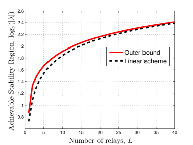
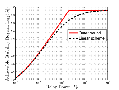
For a symmetric two-hop network with , the gap between necessary and sufficient conditions approaches zero as the number of relays goes to infinity. The gap also monotonically approaches zero as goes to infinity.
Proof V.3
In Fig. 5 we have plotted and as functions of and . These figures show that linear schemes are quite efficient in some regimes.
Remark V.3
Linear policies can be even exactly optimal in the following special cases: i) If we fix all relaying policies to be linear, then the channel becomes equivalent to a point-point scalar Gaussian channel, for which linear sensing is known to be optimal for LQG control [1]. ii) If we fix the state encoder to be linear and assume noiseless causal feedback links from the controller to the relay nodes, then linear policies are optimal for mean-square stabilization over a symmetric two-hop relay network, by the following arguments. Since the control actions are available at the relay nodes via noiseless feedback links, there is no dual effect of control, i.e., the separation of estimation and control holds. Further by restricting the state encoder to be linear, the relay network becomes equivalent to the Gaussian network studied in[48, 45], where it is shown that linear policies are optimal if the network is symmetric.
V-C Non-orthogonal Full-duplex Network
We now consider a non-orthogonal network of full-duplex relay nodes, where all the nodes receive and transmit their signals in every time step, i.e., at any time instant ,
| (24) |
where , , and .
Theorem V.3
If the linear system in (1) is mean-square stable over the non-orthogonal full-duplex relay network, then
| (25) |
where , , , , , , for all .
Proof V.4
The proof follows exactly in the steps of the proof of Theorem V.1, with an exception that odd and even indexed terms are not treated separately because and for all .
Theorem V.4
The scalar linear time invariant system in (1) with and can be mean square stabilized using a linear scheme over the non-orthogonal full-duplex Gaussian network if
| (26) |
where is the unique root in the interval of the following fourth order polynomial
| (27) |
Proof V.5
The proof can be found in [33] for a single relay setup, which can be easily extended for multiple relays.
Although we expect that Theorem V.4 also holds in the presence of process noise like other setups, we are not able to show convergence of second moment of the state process. However numerical experiments suggest that the result should hold.
Remark V.4
The term on the right hand side of the inequality in (26) is an achievable rate with which information can be transmitted reliably over the non-orthogonal full-duplex relay network. This result is derived for a network with single relay node in [49, Theorem 5], however it can be easily extended to problems with multiple relays.
VI Noisy Multi-dimensional Systems
In this section we investigate stabilization of multi-dimensional systems over multi-dimensional channels. First we state a result for a scalar Gaussian channel.
Theorem VI.1
The -dimensional noisy linear system (1) can be mean square stabilized over a scalar Gaussian channel having information capacity , if . Furthermore, a linear time varying policy is sufficient through sequential linear encoding of scalar components.
Proof Outline: We prove Theorem VI.1 with the help of a simple example, due to space limitation in the paper. Consider that a two-dimensional plant with system matrix and an invertible input matrix has to be stabilized over a Gaussian channel disturbed by a zero mean Gaussian noise with variance . We assume that the sensor transmits with an average . For this channel, we define information capacity as . We denote the state and the control variables as and respectively. Consider the following scheme for stabilization. The sensor observes state vector in alternate time steps (that is, at ), whose elements are sequentially transmitted. The sensor linearly transmits at time and at time with an average transmit power constraint. The control actions for the two modes are also taken in alternate time steps, that is, and . Accordingly the state equations for the two modes at time are given by
| (28) | ||||
| (29) |
where and follow from and . The state equations at time are
| (30) | ||||
| (31) |
where follows (29); and follows from . We first study the stabilization of the lower mode. According to (30) the second moment of is given by
| (32) |
where the last equality follows from the linear mean-square estimation of a Gaussian variable over a scalar Gaussian channel of capacity and . We observe that the lower mode is stable if and only if . Assuming that is stable, the second moment of is given by
| (33) |
where follows from (31) and ; follows from the linear mean-square estimation of a Gaussian variable over a scalar Gaussian channel of capacity ; follows from the Cauchy–Schwarz inequality; follows from the fact (assuming that ) and by defining , , and . We now want to a find condition which ensures convergence of the following sequence:
| (34) |
In order to show convergence, we make use of the following lemma.
Lemma VI.1
Let be a non-decreasing continuous mapping with a unique fixed point . If there exists such that and , then the sequence generated by , converges starting from any initial value .
Proof VI.1
The proof is given in Appendix -D.
We observe that the mapping with is monotonically increasing since . It will have a unique fixed point if and only if , since . Assuming that , there exists such that and . Therefore by Lemma VI.1 the sequence is convergent if .
The time sharing scheme illustrated above can be generalized to any -dimensional plant and the stability conditions can be easily obtained using Lemma VI.1. We know that any system matrix can be written in the Jordan form by a similarity matrix transformation. We can then use the following scheme for stabilization. The encoder chooses to send only one component of the observed state vector at each time over a Gaussian channel of capacity . Assume that for a fraction of the total available time the encoder transmits the -th component of the state vector. Thus the rate available for the transmission of the -th state component is . The system will be stable if and only if for all , which implies . For a multi-dimensional system with a controllable pair, any input (control action) can be realized in time steps. If the encoder has access to the channel output, then it can refine estimate of the state using noiseless feedback channel (SK coding scheme) during these time steps and observe the new state periodically after every time steps.
Remark VI.1
Remark VI.2
In [14] the authors studied stabilization of a noiseless multi-dimensional system over a point-to-point scalar Gaussian channel using a linear time invariant scheme, that is the state encoder transmits , where is a row vector. This LTI scheme cannot stabilize if the pair is not observable. For example consider a diagonal system matrix with two equal eigenvalues. This system cannot be stabilized by any choice of the encoding matrix , irrespective of how much power the state encoder is allowed to spend. However our linear time varying scheme can always stabilize the system, even in the presence of process noise.
VII Conclusions
The problem of mean-square stabilization of LTI plants over basic Gaussian relay networks is analyzed. Some necessary and sufficient conditions for stabilization are presented which reveal relationships between stabilizability and communication parameters. These results can serve as a useful guideline for a system designer. Necessary conditions have been derived using information theoretic cut-set bounds, which are not tight in general due to the real-time nature of the information transmission. Sufficient conditions for stabilization of scalar plants are obtained by employing time invariant communication and control schemes. We have shown that time invariant schemes are not sufficient in general for stabilization of multi-dimensional plants. However, a simple time variant scheme is always shown to stabilize multi-dimensional plants. In this time varying scheme, one component of the state vector is transmitted at a time and the state component corresponding to a more unstable mode is transmitted more often. The sufficient conditions for stabilization of multi-dimensional plants are obtained by using this time varying scheme. We also established minimum signal-to-noise ratio requirement for stabilization of a noiseless multi-dimensional plant over a parallel Gaussian channel. It is observed in some network settings that sufficient conditions do not depend on the plant noise and they may be characterized by the directed information rate from the sequence of channel inputs to the sequence of channel outputs. We have discussed optimality of linear policies over the given network topologies. In some very special cases, linear schemes are shown to be optimal.
-A Necessary Condition
Consider the following series of inequalities:
| (35) |
where follows from the definition of directed information; follows from the fact that discarding variables cannot increase mutual information; follows from (1); follows from ; follows from the fact that conditioning reduces entropy; follows from due to mutual independence of and ; follows from [31, Theorem 8.6.4]; follows from conditioning reduces entropy; and follows the fact that for a mean square stable system there exists a matrix with for all and further for a given covariance matrix the differential entropy is maximized by the Gaussian distribution. We can also write
| (36) |
where follows by defining uncontrolled state process and writing the controlled state process as a sum of uncontrolled process and a linear function of control actions , since the system is linear and control actions are additive; and follows from . From (-A) and (-A) we have , since we have assumed .
-B Proof of Theorem V.2
In order to prove Theorem V.2 we propose a linear communication and control scheme. This scheme is based on the coding scheme given in [49] which is an adaptation of the well-known Schalkwijk–Kailath scheme [50]. By employing the proposed linear scheme, we find a condition on the system parameters which is sufficient to mean square stabilize the system (1). The control and communication scheme for the half-duplex network works as follows: If the initial state is not Gaussian distributed, then we first make the state process Gaussian distributed by performing the following initialization step which was introduced in [34].
Initial time step,
At time step , the state encoder observes and it transmits . The decoder receives . It estimates as . The controller then takes an action which results in
| (37) |
The new plant state where .
First transmission phase,
The state encoder observes and transmits . The relay nodes receive this signal over the Gaussian links and do not transmit any signal in this transmission phase due to half-duplex restriction. The decoder observes and computes the MMSE estimate of , which is given by
where () follows from the orthogonality principle of MMSE estimation (that is for ) [51]; () follows from the fact that the optimum MMSE estimator for a Gaussian variable is linear [51]; and () follows from and .
The controller takes an action which results in . The new plant state is a linear combination of zero mean Gaussian variables , therefore it is also zero mean Gaussian with the following variance
| (38) |
where the last equality follows from (by computation).
Second transmission phase,
The encoder observes and transmits . In this phase the relay nodes choose to transmit their own signal to the decoder and thus they cannot listen to the signal transmitted from the state encoder due to the half-duplex assumption. Each relay node amplifies the signal that it had received in the previous time step (first transmission phase) under an average transmit power constraint and transmits it to the decoder . The signal transmitted from the -th relay node is thus given by . The decoder accordingly receives
| (39) |
where , , and is a white Gaussian noise sequence with zero mean and variance . The decoder then computes the MMSE estimate of given all previous channel outputs in the following three steps:
-
1.
Compute the MMSE prediction of from , which is given by , where is the MMSE estimate of .
-
2.
Compute the innovation
(40) where follows from .
-
3.
Compute the MMSE estimate of given . The state is independent of given , therefore we can compute the estimate based only on without any loss of optimality, that is,
(41) where () follows from an MMSE estimation of a Gaussian variable; and () follows from and .
The controller takes action which results in . The new plant state is a linear combination of zero mean Gaussian random variables , therefore it is also zero mean Gaussian distributed with the following variance,
| (42) |
| (43) |
where follows from ; follows by substituting the values of and ; and by substituting using (38) and by defining , , .
We want to find the values of the parameter for which the second moment of the state remains bounded. Rewriting (38) and (43), the variance of the state at any time is given by
| (44) | ||||
| (45) |
where . If the odd indexed sub-sequence in (44) is bounded, then the even indexed sub-sequence in (45) is also bounded. Thus it is sufficient to consider the odd indexed sub-sequence . We will now construct a sequence which upper bounds the sub-sequence . Then we will derive conditions on the system parameter for which the sequence stays bounded and consequently the boundedness of will be guaranteed. In order to construct the upper sequence , we work on the term in (44) and make use of the following lemma.
Lemma .1
([35, Lemma 4.1]) Consider a function defined over the interval , where . The function can be upper bounded as for some , where .
Starting from (44) and by using the above lemma, we write the following series of inequalities
| (46) |
where follows from Lemma .1 and ; and follows from the fact that for all according to (45) and (44). Since in (-B) is a linearly increasing function, it can be used to construct the sequence , which upper bounds the odd indexed sub-sequence given in (44). We construct the sequence for all as
| (47) |
where () follows from (-B) and () follows by recursively apply ().
We observe from (-B) that if , then the sequence converges as and consequently the original sequence is guaranteed to stay bounded. Thus the system in (1) can be mean square stabilized if
| (48) | |||
| (49) |
where the last equality follows from and . Since the relay nodes amplify the desired signal as well as the noise, which is then superimposed at the decoder to the signal coming directly from the state encoder, the optimal choice of the transmit powers depends on the parameters . Moreover, the optimal choice of the power allocation factor at the state encoder also depends on these parameters. Therefore, we rewrite (49) as (21), which completes the proof.
-C Remark V.2 on Information Rate
The given scheme can be seen as a point-point communication channel, where is the channel output corresponding to the input and is the channel output corresponding to the input for . The information rate is given by
| (50) |
where follows from the fact that , the channel is memoryless, the random variables are Gaussian and for , and for all ; and follows from the fact that and are both sequences of i.i.d. variables. For the first transmission phase the mutual information between the transmitted variable and the received variable is given by
| (51) |
where follows from and . In the second phase the decoder computes the innovation according to (40). The mutual information between the transmitted variable and the innovation variable is then given by
| (52) |
where follows from and . From (51), (52), and (-C) the corresponding information rate is equal to
| (53) |
For the given channel, the directed information rate is equal to information rate due to mutual independence of the channel output sequence [38, Theorem 2].
-D Proof of Lemma VI.1
Assume that is a non-decreasing mapping with a unique fixed point . Further assume that there exist such that and . Consider a sequence generated by the following iterations: with , . We want to show that starting from any , the sequence converges. There are three possibilities: i) , ii) , and iii) . For we have , therefore . Since is non-decreasing, . Thus for any we have . Further this sequence is lower bounded by because for any , due to non-decreasing . Thus the sequence converges since it is monotonically decreasing and lower bounded by [52, Theorem 3.14]. For we have , therefore . Since is non-decreasing, we have . Thus for any we have . Further this sequence is upper bounded by because for any , we have due to non-decreasing . Since is strictly increasing and upper bounded by for , it converges [52, Theorem 3.14].
References
- [1] R. Bansal and T. Başar, “Simultaneous design of measurement and control strategies for stochastic systems with feedback,” Automatica, vol. 25, no. 5, pp. 679–694, 1989.
- [2] J. Baillieul, “Feedback designs for controlling device arrays with communication channel bandwidth constraints,” in ARO Workshop on Smart Structures, Aug. 1999.
- [3] W. S. Wong and R. W. Brockett, “Systems with finite communication bandwidth constraints-II: stabilization with limited information feedback,” IEEE Trans. Autom. Control, vol. 44, no. 5, pp. 1049–1053, May 1999.
- [4] G. N. Nair and R. J. Evans, “Stabilization with data-rate-limited feedback: tightest attainable bounds,” Systems & Control Letters, vol. 41, no. 1, pp. 49–56, Sep. 2000.
- [5] N. Elia and S. K. Mitter, “Stabilization of linear systems with limited information,” IEEE Trans. Autom. Control, vol. 46, no. 9, pp. 1384–1400, Sep. 2001.
- [6] G. N. Nair and R. J. Evans, “Stabilizability of stochastic linear systems with finite feedback data rates,” SIAM J. Control Optim., vol. 43, no. 2, pp. 413–436, 2004.
- [7] N. Elia, “When Bode meets Shannon: control–oriented feedback communication schemes,” IEEE Trans. Autom. Control, vol. 49, no. 9, pp. 1477–1488, 2004.
- [8] A. S. Matveev and A. V. Savkin, “The problem of LQG optimal control via a limited capacity communication channel,” Systems & Control Letters, vol. 53, no. 1, pp. 51–64, Sep. 2004.
- [9] S. Tatikonda, A. Sahai, and S. Mitter, “Stochastic linear control over a communication channel,” IEEE Trans. Autom. Control, vol. 49, no. 9, pp. 1549–1561, Sept. 2004.
- [10] S. Tatikonda and S. Mitter, “Control over noisy channels,” IEEE Trans. Autom. Control, vol. 49, no. 7, pp. 1196–1201, 2004.
- [11] N. C. Martins, M. A. Dahleh, and N. Elia, “Feedback stabilization of uncertain systems in the presence of a direct link,” IEEE Trans. Autom. Control, vol. 51, no. 3, pp. 438–447, March 2006.
- [12] A. Sahai and S. Mitter, “The necessity and sufficiency of anytime capacity for stabilization of a linear system over noisy communication links–part I: Scalar systems,” IEEE Trans. Inf. Theory, vol. 52, no. 8, pp. 3369–3395, 2006.
- [13] A. S. Matveev and A. V. Savkin, “An analogue of shannon information theory for detection and stabilization via noisy discrete communication channels,” SIAM J. Control Optim., vol. 46, no. 4, pp. 1323–1367, 2007.
- [14] J. H. Braslavsky, R. H. Middleton, and J. S. Freudenberg, “Feedback stabilization over signal-to-noise ratio constrained channels,” IEEE Trans. Autom. Control, vol. 52, no. 8, pp. 1391–1403, Aug. 2007.
- [15] N. C. Martins and M. A. Dahleh, “Feedback control in the presence of noisy channels: ”Bode-like” fundamental limitations of performance,” IEEE Trans. Autom. Control, vol. 53, no. 7, pp. 1604–1615, Aug. 2008.
- [16] R. H. Middleton, A. J. Rojas, J. S. Freudenberg, and J. H. Braslavsky, “Feedback stabilization over a first order moving average Gaussian noise channel,” IEEE Trans. Autom. Control, vol. 54, no. 1, pp. 163–167, Jan. 2009.
- [17] S. Yüksel and S. Tatikonda, “A counterexample in distributed optimal sensing and control,” IEEE Trans. Autom. Control, vol. 54, no. 4, 2009.
- [18] S. Yüksel and T. Başar, “Control over noisy forward and reverse channels,” IEEE Trans. Autom. Control, vol. 56, pp. 1014–1029, May 2011.
- [19] A. Farhadi and N. U. Ahmed, “Suboptimal decentralized control over noisy communication channels,” Systems Control Letters, vol. 60, pp. 285–293, April 2011.
- [20] C. D. Charalambous, A. Farhadi, and S. Z. Denic, “Control of continuous-time linear Gaussian systems over additive Gaussian wireless fading channels: A separation principle,” IEEE Trans. Autom. Control, vol. 53, no. 4, pp. 1013–1019, May 2008.
- [21] L. Yiqian, E. Tuncel, J. Chen, and S. Weizhou, “Optimal tracking performance of discrete-time systems over an additive white noise channel,” in Proc. IEEE CDC, 2009.
- [22] J. S. Freudenberg, R. H. Middleton, and V. Solo, “Stabilization and disturbance attenuation over a Gaussian communication channel,” IEEE Trans. Autom. Control, vol. 55, no. 3, pp. 795–799, March 2010.
- [23] Z. Shu and R. H. Middleton, “Stabilization over power-constrained parallel Gaussian channels,” IEEE Trans. Autom. Control, vol. 56, no. 7, pp. 1718–1724, July 2011.
- [24] S. Yüksel, “Characterization of information channels for asymptotic mean stationarity and stochastic stability of non-stationary/unstable linear systems,” IEEE Trans. Inf. Theory, vol. 58, no. 10, pp. 6332–6354, Oct. 2012.
- [25] E. I. Silva, G. C. Goodwin, and D. E. Quevedo, “Control system design subject to SNR constraints,” Automatica, vol. 46, no. 2, pp. 428–436, 2010.
- [26] F. J. Vargas, E. I. Silva, and J. Chen, “Stabilization of TITO systems over parallel SNR-constraint AWN channels,” in Proc. 7th IFAC Symposium on Robust Control Design, 2012.
- [27] U. Kumar, V. Gupta, and J. N. Laneman, “On stability across a Gaussian product channel,” in IEEE CDC, December 2011, pp. 3142–3147.
- [28] V. A. Vaishampayan, “Combined source-channel coding for bandlimited waveform channels,” Ph.D. dissertation, University of Maryland, 1989.
- [29] S. Tatikonda, “Some scaling properties of large distributed control systems,” in IEEE CDC, Dec. 2003, pp. 3142–3147.
- [30] V. Gupta, A. F. Dana, J. P. Hespanha, R. M. Murray, and B. Hassibi, “Data transmission over networks for estimation and control,” IEEE Trans. Autom. Control, vol. 54, no. 8, pp. 1807–1819, Aug. 2009.
- [31] T. Cover and J. Thomas, Elements of information theory. John Wiley Sons, Inc., 2006.
- [32] M. Gastpar and M. Vetterli, “On the capacity of large Gaussian relay networks,” IEEE Trans. Inf. Theory, vol. 51, no. 3, pp. 765–779, March 2005.
- [33] A. A. Zaidi, T. J. Oechtering, and M. Skoglund, “Rate sufficient conditions for closed–loop control over AWGN relay channels,” in IEEE ICCA, June 2010, pp. 602–607.
- [34] A. A. Zaidi, T. J. Oechtering, S. Yüksel, and M. Skoglund, “Closed-loop control over half-duplex AWGN relay channels,” in Reglermöte, June 2010.
- [35] ——, “Sufficient conditions for closed-loop control over a Gaussian relay channel,” in IEEE ACC, June 2011, pp. 2240–2245.
- [36] U. Kumar, V. Gupta, and J. N. Laneman, “Sufficient conditions for stabilizability over Gaussian relay channel and cascade channels,” in IEEE CDC, December 2010, pp. 4765–4770.
- [37] E. I. Silva, M. S. Derpich, and J. Ostergaard, “A framework for control system design subject to average data-rate constraints,” IEEE Trans. Autom. Control, vol. 56, no. 8, pp. 1886–1899, Aug. 2011.
- [38] J. L. Massey, “Causality, feedback and directed information,” in IEEE ISITA, 1990.
- [39] A. A. Zaidi, S. Yüksel, T. J. Oechtering, and M. Skoglund, “On optimal policies for control and estimation over a Gaussian relay channel,” in IEEE CDC, 2011.
- [40] G. M. Lipsa and N. C. Martins, “Optimal memoryless control in Gaussian noise: A simple counterexample,” Automatica, vol. 47, pp. 552–558, March 2011.
- [41] D. Tse and P. Viswanath, Fundamentals of Wireless Communication. Cambridge University Press, 2005.
- [42] N. Wernersson and M. Skoglund, “Nonlinear coding and estimation for correlated data in wireless sensor networks,” IEEE Trans. Commun., vol. 57, no. 10, pp. 2932–2939, October 2009.
- [43] S. Shamai, S. Verdu, and R. Zamir, “Systematic lossy source/channel coding,” IEEE Trans. Inf. Theory, vol. 44, no. 2, pp. 564–579, March 1998.
- [44] M. Andersson, A. A. Zaidi, N. Wernersson, and M. Skoglund, “Nonlinear distributed sensing for closed-loop control over Gaussian channels,” in IEEE Swe–CTW, October 2011, pp. 19–23.
- [45] M. Gastpar, “Uncoded transmission is exactly optimal for a simple Gaussian sensor network,” in Information Theory and Applications Workshop, 2007.
- [46] J.-J. Xiao, S. Cui, Z.-Q. Luo, and A. J. Goldsmith, “Linear coherent decentralized estimation,” IEEE Trans. Signal Processing, vol. 56, no. 2, pp. 757–770, Feb. 2008.
- [47] S. Tatikonda, S., and Mitter, “The capacity of channels with feedback,” IEEE Trans. Inf. Theory, vol. 55, no. 1, pp. 323–349, Jan. 2009.
- [48] M. Gastpar, “Uncoded transmission is exactly optimal for a simple Gaussian sensor network,” IEEE Trans. Inf. Theory, vol. 54, pp. 5247–5251, 2008.
- [49] S. Bross and M. Wigger, “On the relay channel with receiver-transmitter feedback,” IEEE Trans. Inf. Theory, vol. 55, no. 1, pp. 275–291, 2009.
- [50] Schalkwijk and T. Kailath, “A coding scheme for additive noise channels with feedback–I: No bandwidth constraint,” IEEE Trans. Inf. Theory, vol. 12, no. 2, pp. 172–182, 1966.
- [51] M. Hayes, Statistical digital signal processing and modelling. John Wiley Sons, Inc., 1996.
- [52] W. Rudin, Principles of Mathematical Analysis. McGraw-Hill Book Company, 1976.