Anti-Levitation in the Integer Quantum Hall Systems

Abstract

The evolution of extended states of two-dimensional electron gas with white noise randomness and field is numerically investigated by using the Anderson model on square lattices. Focusing on the lowest Landau band we establish an anti-levitation scenario of the extended states: As either the disorder strength $W$ increases or the magnetic field strength $B$ decreases, the energies of the extended states move below the Landau energies pertaining to a clean system. Moreover, for strong enough disorder, there is a disorder dependent critical magnetic field $B_{c}(W)$ below which there are no extended states at all. A general phase diagram in the $W-1/B$ plane is suggested with a line separating domains of localized and delocalized states.

I Introduction

Energies of an electron in a clean two-dimensional system subject to a strong perpendicular magnetic field $B$ form sharp Landau levels at energies $\varepsilon_{n}=(n+1/2)\hbar\omega_{c}$, $n=0,1,2,\ldots$ [where $\omega_{c}=eB/(mc)$] and the corresponding eigenstates (Landau functions) are extended. If the system is moderately disordered, for example by a white-noise random on-site energy of zero mean and fluctuation strength $W$ such that $W<\hbar\omega_{c}$, the Landau levels are broadened to form separated Landau bands (LBs).[1] The density of states of each LB is maximal around its center $E_{n}$.[2] While the (possibly degenerate) eigenstates at energy $E_{n}$ are still extended, states at energies $\varepsilon\neq E_{n}$ are localized. This is the origin of the integer quantum Hall effect (IQHE).[3] The question of whether $E_{n}=\varepsilon_{n}$ is one of the topics discussed in this work. Each LB $i$ is characterized by a topological (Chern) integer $\nu_{i}$,[4] and the Hall conductivity $\sigma_{xy}$ at Fermi energy $E_{n}<\varepsilon_{F}<E_{n+1}$ is equal to $\sum_{i=1}^{n}\nu_{i}$ in the unit of $e^{2}/h$. Strictly speaking, only extended states at energy $E_{i}$ within each LB contribute to its Chern number. Chern numbers cannot be created or destroyed by an adiabatic change of $B$ or $W$.

One of the fundamental issues in the physics of the IQHE is to elucidate the evolution of extended states in LBs with stronger disorder and/or weaker magnetic field such that the inequality $W<\hbar\omega_{c}$ is no longer strictly satisfied. As $B\to 0$ all electronic states in a disordered two-dimensional system are localized [5] and for $B=0$ there are neither LB nor Chern numbers. On the other hand, a LB with Chern number $\nu$ cannot lose it unless it is annihilated by an opposite Chern number $-\nu$ belonging to another LB. In Refs. 6, 7, 8 the scenario of Chern number annihilation as $B\to 0$ has been discussed on a qualitative level. In order to add more quantitative perception, it is vital to elucidate the behavior of extended states in LBs as the magnetic field gradually decreases to zero, or as the disorder gradually increases. Different answers to this question lead to different global phase diagrams [6, 7, 8] for the IQHE.

In the absence of spin-orbit interaction, the prevailing paradigm (assuming 2D continuum geometry) is that when $B\to 0$, all extended states float up to infinite energy. The quantitative form of this levitation scenario [9, 10] states that the energy of an extended state in the $n$th LB goes like

$$\begin{split}E_{n}=\varepsilon_{n}[1+(\omega_{c}\tau)^{-2}],\end{split}$$ (1)

where $\tau$ is the impurity scattering time. Thus, extended states float upward as $\omega_{c}\rightarrow 0$ or $\tau\rightarrow 0$.[11] As far as experiments are concerned, the levitation scenario is still not settled. Some experiment support it [12, 13, 14, 15] and others do not.[16, 17] Some theoretical works based on continuous 2D geometry treat the levitation scenario using numerous approximation methods as well as various numerical calculations. [11, 18, 19, 20, 21] Most of them support the general idea although there is no strict evidence that extended states float up to infinity. Numerical simulations on a lattice are also not conclusive. For white-noise random on-site energy, levitation is not substantiated [7] while for finite range correlated disorder, weak levitation is predicted.[22, 23, 24]

In this paper we revisit this issue by focusing on the evolution of extended states in the lowest LB ($n=0$) using a square lattice geometry and white-noise random on-site energy. The lattice geometry is especially useful at low magnetic field where LBs strongly overlap. Our main result (to be substantiated below) is that under these conditions, extended states in the lowest LB plunge down instead of floating up when $\omega_{c}\tau\to 0$. This anti-levitation behavior is schematically displayed in Fig. 1 and contrasted with the levitation scenario encoded in Eq. (1).

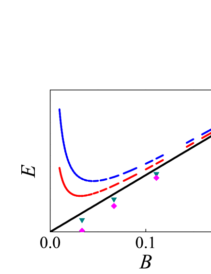
Figure 1: (Color online) Schematic picture of the anti-levitation scenario (obtained from a solution of the lattice model with white-noise distribution of site disorder), contrasted with the levitation scenario formulated in Eq. (1). Energies of extended states on the lowest LB are shown as a function of the magnetic field for different cases. (1) Clean system in the continuous geometry (solid line) where the energy follows the relation $E_{0}=\frac{1}{2}\hbar\omega_{c}$. (2) Disordered systems in the continuous geometry following Eq. 1 for $\tau_{1}$ (lower dashed line) $>\tau_{2}$ (upper dashed line). (3) Disordered system in the lattice geometry with white-noise random on-site energy for disorder strengths $W_{1}$ (triangles) $<W_{2}$ (diamonds). Anti-levitation occurs for fixed $B$ with increasing $W$ and for fixed $W$ with decreasing $B$.

This anti-levitation scenario is consistent with the concept of level repulsion as explained below. It is substantiated by two independent numerical approaches. In the first one, the extended state energy is identified as the critical energy for the IQHE plateaux transition where the localization length diverges. The second one is based on the calculation of the participation ratio (PR).

This paper is organized as follows. In the first part of Sec.II, the model describing an electron on a 2D square lattice with white-noise disorder under a perpendicular magnetic field is very briefly discussed. In the second part of Sec.II we give, for the sake of self-consistence, a short explanation of the transfer matrix and PR methods designed to locate the extended state energies $E_{n}$. Section III is devoted to presentation of the numerical results and their analysis, while a short summary is presented in Sec.IV.

II Model and Methods

We consider a tight-binding Hamiltonian on a square lattice,

$$\begin{split}H=\sum_{i}\epsilon_{i}a_{i}^{\dagger}a_{i}+\sum_{<ij>}\exp(i\phi_{ij})a_{i}^{\dagger}a_{j}.\end{split}$$ (2)

Here $i=(n_{i}a,m_{i}a)$ is a point on a square lattice of lattice constant $a$, where $1\leq n_{i}\leq L$ and $1\leq m_{i}\leq M$ ($n_{i},m_{i},L,M$ are nonnegative integers), and $a_{i}^{\dagger},a_{i}$ are electron creation and annihilation operators on site $i$. The on-site energy $\epsilon_{i}$ on site $i$ is a random number uniformly distributed in the range of $[-\frac{W}{2},\frac{W}{2}]$. Thus, $W$ measures the degree of randomness. The symbol $<ij>$ indicates that $i$ and $j$ are nearest-neighbor sites. The magnitude of the hopping coefficient (prefactor of the exponent) is used as an energy unit. The magnetic field is introduced through the Peierls substitution [25] by adding a phase $\phi_{ij}=2\pi(e/h)\int_{i}^{j}\vec{A}\cdot d\vec{l}$ to the hopping coefficient. The vector potential is chosen as $\vec{A}=(0,Bx,0)$ for a uniform magnetic field $\vec{B}$ along the $z-$direction, where $B$ is in the units of flux quantum $e/h$ per plaquette. Under this gauge, the nonzero phase exists only on bonds along the $y-$direction. The energy range of eigenstates for a pure system is $[-4,4]$. In the presence of mild disorder potential, the energy spectrum slightly extends beyond $[-4,4]$. Because the model (2) has particle-hole symmetry, the discussion below can be restricted within the energy range $[-4,0]$.

To locate the extended state energies at a given magnetic field $B$ and disorder fluctuation energy range $W$, we use two independent approaches. The first one is the transfer matrix method. The electron is scattered from a quasi-one-dimensional lattice (a strip) of length $La\to\infty$ and width $Ma$ with $L\gg M$. Assume that the $x-$axis lies along the longitudinal direction of the strip and the $y-$axis along its transverse direction; the transfer matrix transforms the amplitudes of the wave function on sites $(a,ma)$ to its amplitudes on sites $(La,ma)$ ($m=1,2,\ldots,M$). From the eigenvalues of the transfer matrix one can effectively compute the localization length $\lambda_{M}(E)$ of the scattering state at energy $E$.

In order to avoid the edge effect, periodical boundary conditions are imposed on the $y-$direction. Let us denote by $\psi_{n}$ the vector of $M$ wave function amplitudes on the $n^{th}$ column of the lattice, namely, $\psi_{n}=(\psi_{n,1},\psi_{n,2},\ldots,\psi_{n,M})^{T}$. Following the method specified in Ref. 26, the $2M$ vector of wave function amplitudes $(\psi_{n+1},\psi_{n})^{T}$ is related to the vector $(\psi_{n},\psi_{n-1})^{T}$ according to the relation

$$\begin{split}\begin{bmatrix}\psi_{n+1}\\ \psi_{n}\end{bmatrix}=\begin{bmatrix}E-H_{n}&-I\\ I&0\end{bmatrix}\begin{bmatrix}\psi_{n}\\ \psi_{n-1}\end{bmatrix}\equiv T_{n}\begin{bmatrix}\psi_{n}\\ \psi_{n-1}~{}.\end{bmatrix}\end{split}$$ (3)

where $I$ is $M\times M$ identity matrix and the matrix $H_{n}$ is the part of Hamiltonian related to the $n$th column. The $2M\times 2M$ transfer matrix is given by the product $T\equiv\prod_{n=1}^{L}T_{n}$. For $L\to\infty$ the $2M$ eigenvalues of $T$ (Lyapunov exponents) can be approximated as $e^{\pm L/\xi_{m}(E)}$ where Re$[\xi_{m}(E)]\geq 0$.[26] The localization length $\lambda_{M}(E)$ is given by $\lambda_{M}(E)$=Max_mRe$[\xi_{m}(E)]$. In our calculations the strip length is chosen to be $10^{6}$, much larger than $\lambda_{M}$, to take the advantage of self-averaging.

In order to obtain the localization length $\xi(E)=\lambda_{M\to\infty}(E)$ of an infinite 2D system from the localization length $\lambda_{M}$ of finite systems, we employ the single parameter scaling ansatz [27, 28] implying that for a large enough system $\lambda_{M}/M$ depends only on a single parameter $M/\xi(E)$; i.e.,

$$\begin{split}\frac{\lambda_{M}(E)}{M}=f\left(\frac{M}{\xi(E)}\right).\end{split}$$ (4)

If there is a mobility edge $E_{c}$ that separates localized states from extended states, then scaling theory says

$$\begin{split}\xi(E)\propto|E-E_{c}|^{-\nu},\end{split}$$ (5)

where $\nu$ is a universal critical exponent depending only on dimensionality and symmetries. According to Eq. (4), $\lambda_{M}(E)/M$ of different $M$ shall all cross at $E=E_{c}$ when extended states for a band or merge there if the state of energy $E_{c}$ is an isolated extended state. Thus, crossing or mergence of curves of $\lambda_{M}(E)/M$ for different $M$’s is a feature for extended states. Equation ( 4) has the following asymptotic limits: $f(x)\propto 1/x$ for $M\to\infty$ and $f(x)\simeq f(0)$ when $E\to E_{c}$.

An alternative approach to study localized and extended states is to compute the participation ratio (PR) of an eigenstate $\psi_{E}(\vec{x})$ with energy eigenvalue $E$. In a lattice geometry, it is defined as [24, 29, 2]

$$\begin{split}\mbox{PR}(E)=\frac{1}{N\sum_{i}|\psi_{E}(i)|^{4}},\end{split}$$ (6)

where $N$ is the total number of lattice sites and $\psi_{E}(i)$ is the amplitude of a normalized wave function at site $i$. The PR is of order of $1/N$ for a maximally localized state ($|\psi_{E}(i)|=\delta_{i,i_{0}}$), and of order of $1$ for a maximally extended (uniform) state ($|\psi_{E}(i)|=1/\sqrt{N}$). For an extended state whose wave function is a fractal [30] of dimension $D$, its PR should scale with $N$ as $N^{-1+D/2}$. Note that a localized state scales as $N^{-1}$; namely its fractal dimension is $D=0$. Numerically, however, the distinction between a fractal state and a localized state requires calculations on a large enough lattice. Here, we will use PR mainly to consistently check the information obtained from the transfer matrix calculations. More concretely, a local peak of PR($E$) at an energy $\bar{E}$ indicates that the state $\psi_{\bar{E}}$ is less localized than its neighboring states $\psi_{E\neq\bar{E}}$. Based on the transfer matrix method, we may deduce that the state $\psi_{\bar{E}}$ is extended. Practically we shall diagonalize the Hamiltonian (2) on an $M\times M$ square lattice with $M$ up to 100 and compute PR$(E)$ for all energy eigenstates according to the above definition.

III Results

In the first part of this section we trace the location of the extended state energies on the lowest LB for a fixed magnetic field and varying disorder strength $W$, while in the second part we analyze their location for a fixed disorder and varying magnetic field, and then draw a “phase diagram” of the lowest LB in the $W-1/B$ plane.
 

III.1 Fixed $B$ and increasing $W$

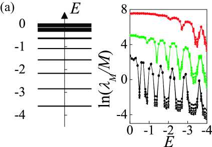
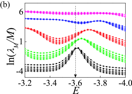
Figure 2: (Color online) (a) The left panel illustrates the eight Landau subbands in the energy range $[-4,0]$ for a clean system for $B=1/15$. The right panel displays the quantity $\ln(\lambda_{M}/M)$ as a function of energy $E$ for a fixed magnetic field $B=1/15$ (expressed in quantum flux per square) in the same energy range for (from bottom up) $W$=1 (black), 2 (green), 3 (red). The numerical data of $\ln(\lambda_{M}/M)$ are obtained by averaging over 40 samples. Bundles of curves for $W=n$ ($n$=2,3) are shifted upward by 2$n$. In each bundle, the system widths are $M=32$ (square), 48 (circle), 64 (up-triangle), 80 (down-triangle) and 96 (left-triangle). (b) As in the right panel of (a), but here $\ln(\lambda_{M}/M)$ is displayed in the energy range of $[-4,-3.2]$ for (from bottom up) $W$=1 (black), 2 (green), 3 (red), 4 (blue), 5 (pink). Bundles of curves for $W=n$ ($n$=2,3,4,5) are shifted upward by 1.5$n$. The dash arrow indicates the location of extended state of a clean system with $B=1/15$.

First, we focus on the existence and evolution of extended state(s) in the lowest LB as $B$ (expressed in units of quantum flux per square) is fixed and $W$ increases. The results of this part elaborate upon earlier ones reported in Ref. 31. For comparison, the left panel of Fig. 2(a) illustrates the eight Landau subbands in the energy range $[-4,0]$ for a clean system with $B=1/15$ since the electron spectrum is mirror symmetric about $E=0$. The right panel of Fig. 2(a) displays the values of $\ln(\lambda_{M}/M)$ vs $E$ for $B=1/15$, $W=1,2,3,4,5$, and $M=32,\ 48,\ 64,\ 80,\ 96$ in the same energy range ($E\in[-4,0]$). Figure 2(b) displays the results of $\ln(\lambda_{M}/M)$ vs. $E$ for $B=1/15$, $W=1,2,3,4,5$, and $M=32,\ 48,\ 64,\ 80,\ 96$ in a smaller energy range of $E\in[-4,-3.2]$ for the lowest Landau band (thus achieving higher resolution). Within each bundle of curves (corresponding to a given value of disorder $W$), the condition

$$M_{1}>M_{2}\ \Rightarrow\ln(\lambda_{M_{1}}(E)/M_{1})<\ln(\lambda_{M_{2}}(E)/M_{2}),$$ (7)

indicates a localized state at energy $E$. For $W=1,2,3,4$, the curves in each bundle for different $M$ merge at the peaks, and at the corresponding energy $E_{c}$ the quantity $\ln(\lambda_{M}(E_{c})/M)$ is independent of $M$. At the critical points $E_{c}(W)$, the values of $\lambda_{M}/M$ are nearly the same besides some numerical errors. Within the one-parameter scaling ansatz, this indicates quantum Hall transitions between localized states and isolated extended (critical) states at $E_{c}$. The value of $E_{c}(W)$ depends on $W$, explicitly $E_{c}(1)=-3.619,\ E_{c}(2)=-3.651,\ E_{c}(3)=-3.718,\ E_{c}(4)=-3.771$. It should be pointed out that the seemingly merging point near $E=-3.2$ for $W=3$ and above in Fig. 2(b) is near the extended state of the second lowest Landau band.

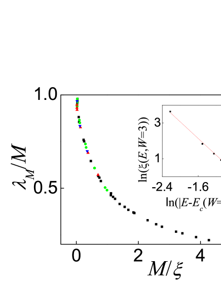
Figure 3: (Color online) The scaling function $\lambda_{M}/M=f(x=M/\xi)$ for $B=1/15$ and $W=1$ (black square), 2 (green circle), 3 (red up-triangle), 4 (blue down-triangle). The data points are from the critical regime (around the peaks) of Fig. 2(b). Inset: The localization length $\ln(\xi(E,W=3))$ as a function of $\ln(|E-E_{C}(W=3)|)$ for $E_{c}(W=3)=-3.718$. The solid line is linear fit with slope $\nu$=2.34.

To substantiate that quantum phase transitions happen indeed at $E_{c}$’s, we show in Fig. 3 that all curves around the peaks of $W=1,\ 2,\ 3,\ 4$ in Fig. 2(b) collapse on a single smooth curve $f(x)$ with $x=M/\xi(E,W)$ when a proper $\xi(E,W)$ is chosen. Furthermore, $\xi(E,W)$ diverges at $E=E_{c}(W)$ as a power law $\xi\sim[E-E_{c}(W)]^{-\nu}$. The inset of Fig. 3 is the curve of $\ln\xi$ vs $\ln(E-E_{c})$ for $W=3$ with $E_{c}=-3.718$. The nice linear fit with slope $\nu=2.34$ is a strong support of the one-parameter scaling theory. This value is slightly smaller than the latest estimate $\nu=2.59$,[32] but it agrees with the estimation $\nu=2.34\pm 0.04$ [33] for the lowest LB. Thus, from the one-parameter finite-size scaling analysis it is concluded that the state(s) at $E_{c}$ for $W=1,\ 2,\ 3,\ 4$ are extended while states near (but away from) $E_{c}$ are localized.

While for $W=4$ the peak at $E_{c}$ at which the curves merge is still visible (although it is very shallow), we see that for the bundle of curves corresponding to $W=5,\ B=1/15$ there is no peak and the curves $\lambda_{M}/M$ do not merge. If this bundle of curves for $W=5$ is inspected at higher resolution, it is found that the inequality (7) is valid at all energies. This indicates the absence of Hall transition for $W=5$. Inspecting $E_{c}(W)$ from Fig. 2(b), we see that, for a fixed magnetic field ($B=1/15$ in this case) the energy of the extended states on the lowest LB plunges down as $W$ increases (from $E_{c}=-3.619$ at $W=1$ to $E_{c}=-3.771$ at $W=4$) and then disappears for a strong enough disorder ($W=5$). We refer to this slightly downward trend of $E_{c}(W)$ on the lowest LB as disorder-driven anti-levitation. It contrasts the levitation picture conjectured for continuous systems. [9, 10] It is also slightly distinct from the picture conjectured in previous works within the lattice geometry,[7] where it is argued that $E_{c}(B,W)=\varepsilon_{0}(B)$ before the states become localized at higher $W$.

The disappearance of the level $E_{c}(W)$ of extended states on the lowest LB at strong disorder raises the question of what happens with the Chern number attached to that level. The answer to this question is conjectured in Ref. 7: At strong disorder $W$ two levels with opposite Chern numbers approach each other and eventually annihilate each other. Quantitative substantiation of this conjecture falls beyond the scope of the present study.

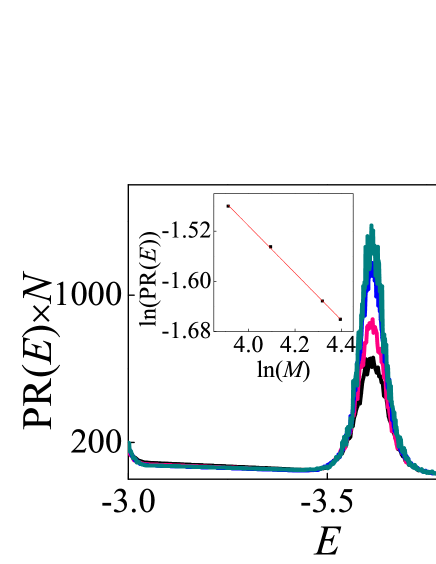
Figure 4: (color online) Averaged PR$\times N$ as a function of energy $E$ for fixed magnetic field $B=1/15$ and disorders $W=1$. The lattice size (from down top) is $51\times 51$ (black), $61\times 61$ (pink), $75\times 75$ (blue), $81\times 81$ (cyan). The calculation is averaged for 40 samples. Inset: The $\log$(PR) as a function of $\log(M)$ for $E=-3.621$. The corresponding solid lines are the linear fit of the data with a slope $-0.39$.

Let us now inspect the disorder-driven anti-levitation using the PR method, that implies the calculation of the wave functions $\psi_{E}(i)$ that live on an $M\times M$ square lattice, and calculating the relevant PR. Figure 4 shows PR$\times N$ ($N=M\times M$) as a function of energy for fixed magnetic field $B=1/15$ and disorder $W=1$ of lattice size of (top down) $51\times 51$ (black), $61\times 61$ (pink), $75\times 75$ (blue), $81\times 81$ (cyan). Focusing on the first LB, the highest PR$\times N$ appears at energy $-3.621$, independent of the sample size, for $W=1$ and $B=1/15$. Unlike the $\lambda_{M}/M$ curves, the PR$\times N$ curves for different sample sizes do not cross. The PR$\times N$ peak energies virtually coincide with $E_{c}(1)=-3.619$ obtained within the transfer matrix method. Thus, the energy of the highest PR$\times N$ in the first LB is consistent with $E_{c}(W)$ discussed within the one-parameter finite size scaling hypothesis. One can further see that PR$\times N$ peaks indeed correspond to extended states by studying the sample size dependence of peak heights and PR$\times N$ at other energies. Focusing on Fig. 4, first one can clearly see that at the energy far from the peak energy $E_{c}(1)=-3.621$ the PR$\times N$ is $M$ independent which implies $D=0$ for these energies. Namely, these states are localized. Second, at the peak energy $E_{c}(1)=-3.621$, the PR$\times N$ increases with $M$. The inset of Fig. 4 is the natural logarithm plot of the PR vs sample size $M$ at the peak with an exponent of $-0.39$, indicating a fractal wave function of dimension $D=2-0.39=1.61$ for the peak. This result is consistent with the multifractal analysis of the integer quantum Hall effect [34] where it is found that the fractal dimension of extended states on the first LB is $D=1.6$. Third, at energies slightly different from the peak $E_{c}(1)=-3.621$ the curves PR$\times N$ do not merge for small $M$ ($M=51$ and $M=61$) but merge for larger $M$ ($M=75$ and $M=81$). For a large enough system the PR$\times N$ should merge together for different $M$ at all energy (localized states) except for the peak (extended states). Since the energy of the peak is size-independent, anti-levitation can be derived without resorting to finite size scaling analysis. However, for the calculation of the critical exponent $\nu$ one must employ finite-size scaling analysis either within transfer matrix formalism or within PR analysis.

In Ref. 31 the authors calculate the Hall conductivity and the localization length for white noise and also for short range correlated disorder. For the white-noise disorder the disorder-driven anti-levitation scenario is found while for the finite-range correlated disorder a weak levitation is noticed. An indirect substantiation of the disorder-driven anti-levitation scenario for Gaussian white noise on-site potential can also be found by analyzing the results in Ref. 35. The authors calculated $\sigma_{xx}$ and $\sigma_{xy}$ for a lattice geometry. By inspecting their results at $B=1/6$ it can be seen that the first plateau transition occurs at an energy $E_{c}\approx-3.18$ that is lower than the energy of the lowest Landau level in a clean system ($\varepsilon_{0}\approx-3.09$).

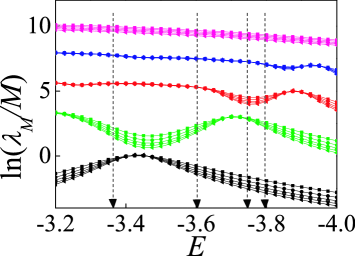
Figure 5: (Color online) The figure displays $\ln(\lambda_{M}/M)$ (averaged over $40$ samples) as a function of energy $E$ for fixed disorder strength $W=3$ at different magnetic fields. The curve bundles from bottom up correspond to $B=1/9$ (black), $1/15$ (green), $1/24$ (red), $1/30$ (blue), and $1/40$ (pink). In order to have a better view, bundle of curves of $B=1/15$ is shifted upward by 3 relative to those of $B=1/9$. The bundles of $B=1/24$, $B=1/30$, and $B=1/40$ are then shifted upward by 2 in order. In each bundle, the system width is $M=32$ (square), $48$ (circle), $64$ (upper triangle), $80$ (down triangle), $96$ (left triangle). The dashed arrows indicate the locations of extended states (from left to right) of clean systems with $B=1/9$, 1/15, 1/24, and 1/30, respectively.

III.2 Fixed $W$ and decreasing $B$

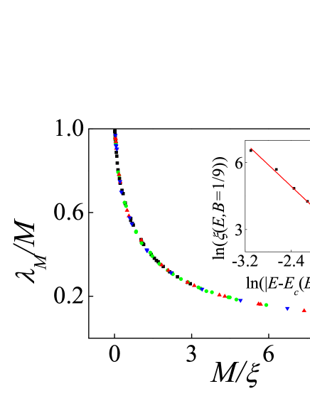
Figure 6: (Color online) The scaling function $\lambda_{M}/M=f(x=M/\xi)$ for $W=3$ and $B=1/9$ (black square) ,1/15 (green circle) ,1/24 (red up-triangle) ,1/30 (blue down-triangle). The data points are from the critical regime (around the peaks) of Fig. 5. Inset: The localization length $\ln(\xi(E,B=1/9)$ as a function of $\ln(|E-E_{C}(B=1/9)|)$ for $E_{C}(B=1/9)=-3.444$. The solid line is linear fit with slope $\nu$=2.34.

Next, we address the effect of decreasing magnetic field on the first extended state(s) at a fixed moderate disorder. Assuming the effect of increasing disorder and lowering magnetic field on the behavior of energies of extended states enters through the dimensionless parameter $\omega_{c}\tau$ it is natural to inspect anti-levitation at fixed $W$ and decreasing $B$. However, we are unaware of similar analysis, (for example, in Ref. 31 $B$ is fixed and $W$ is changed). In Fig. 5, the average $\ln(\lambda_{M}/M)$ is displayed versus energies for $W=3$, different system widths $M=32,\ 48,\ 64,\ 80,\ 96,$ and magnetic fields $B=1/9,\ 1/15,\ 1/24,\ 1/30$. Curve bundles for $B>1/30$ display peaks at which $\ln(\lambda_{M}/M)$ are merged for different $M$. At the merge points, the values of $\lambda_{M}/M$ of different bundles are the same. The mergence is confirmed by the finite-size scaling analysis that all data around the peaks collapse onto a single smooth curve, $\lambda_{M}/M=f(x=M/\xi(E,B))$, as shown in Fig. 6 when a proper $\xi(E,B)$ is used. Indeed the scaling functions in Fig. 3 and Fig. 6 are exactly the same (they overlap with each other) and they are also the same as in Fig. 15 of Ref. 1, implying the scaling function is universal in the integer quantum Hall system. Furthermore, the extracted $\xi(E,B)$ diverges in a power-law fashion at energy $E_{c}$ whose value changes with $B$ as shown in the inset of Fig. 6 with the critical exponent of $\nu=2.34$, the same as the one found earlier. The numerical critical energies are $E_{c}=-3.444$ for $B=1/9$, $-3.712$ for $B=1/15$, $-3.901$ for $B=1/24$, and $-3.955$ for $B=1/30$. The corresponding states at these energies are extended (or, more precisely, critical). The values of $E_{c}=-3.404$ for $B=1/9$ and $E_{c}=-3.718$ for $B=1/15$ are consistent with those at the peak positions obtained through the PR calculations shown in Fig. 7.

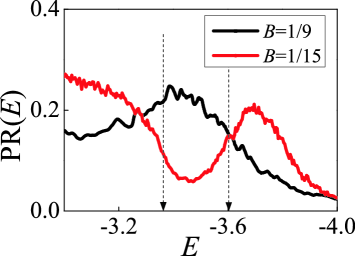
Figure 7: (Color online) Averaged PR as function of energy $E$ for a fixed disorder ($W=3$) and two different green magnetic fields $B=1/9$ (square) and $B=1/15$ (circle). The lattice size is chosen as $81\times 81$ square lattice. The calculation is averaged for 40 samples. The dash arrows indicate the locations of extended states of a clean system with $B=1/9$ (left) and $B=1/15$ (right).

Remarkably, at lower magnetic field, for example $B=1/40$ in Fig. 5, the corresponding bundle of curves does not have a peak, and when inspected with higher resolution, its curves for different $M$ follow inequality (7). In other words, there is a critical (disorder dependent) magnetic field $B_{c}(W)$ below which the extended states on the lowest LB become localized. This is qualitatively consistent with the results of Ref. 7. There is, however a difference between our results and those of Ref. 7 regarding the behavior of the critical energy $E_{c}(B,W)$ for $B>B_{c}(W)$. We arrive at the somewhat unexpected result that with decreasing magnetic field $E_{c}(B,W)$ plunges down faster than $\varepsilon_{0}(B)$ (the lowest Landau level in Hofstadter’s butterfly [36] that is a decreasing function of $B$). In short, for $B\geq B_{c}(W)$ we find $E_{c}(B,W)<\varepsilon_{0}(B)$ and eventually, for $B<B_{c}(W)$, there are no extended states on the lowest LB. We refer to this scenario as magnetic-field-driven anti-levitation. The qualitative explanation of Chern number annihilation mechanism suggested in Ref. 7 applies here as well. The essential results of our extensive numerical calculations are displayed in Fig. 8, which shows the deviation $E_{c}(B,W)-\varepsilon_{0}(B)$ between the first extended state(s) energy and the center of the first LB with varying disorder and magnetic field. An obvious anti-levitation of the first extended state(s) energy $E_{c}(B,W)$ can be observed at strong disorder and/or for weak magnetic field.

The magnetic-field-driven anti-levitation can be understood following the principle of level repulsion or avoided crossing. Assume $E_{c}$ is the energy of the extended state in the lowest LB for a fixed field $B$; when the random potential of zero mean increases by $\Delta V$, the energy shift of the extended state at the second-order perturbation is

$$\begin{split}\Delta E_{c}=\sum_{E\neq E_{c}}\frac{|\langle E|\Delta V|E_{c}\rangle|^{2}}{E_{c}-E},\end{split}$$ (8)

Here $|E_{c}\rangle$ is an extended state on the lowest LB at energy $E_{c}$ and $|E\rangle$ denotes an arbitrary state (possibly localized, and including higher Landau bands) at energy $E\neq E_{c}$. Note that both $|E_{c}\rangle$ and $|E\rangle$ correspond to the “unperturbed” system at potential $V$. We also assume that $V$ is strong enough to lift the degeneracy of the lowest LB, justifying the use of non degenerate perturbation theory. It is expected that the contribution from localized states will be much smaller than that of the extended ones, and therefore, assuming that the states $E_{c}$ are extended and belong to higher LB. Since $E_{c}$ is located around the LB center, there are more states whose energies are above $E_{c}$ than those below $E_{c}$. Thus, more terms in the sum are negative, and $\Delta E_{c}<0$, implying anti-levitation. According to Eq. (8), the shift should be proportional to $W^{2}$. This is indeed consistent with our numerical data points that agree with quadratic fits $\Delta E_{c}=-a(B)W^{2}$ (dashed lines in Fig. 8). As for the dependence of $\Delta E$ on $B$ for fixed $W$, we note that the denominator on the right-hand side of Eq. (8) is approximately proportional to the Landau level spacing (recall that $|E\rangle$ belongs to higher LB). This suggests an estimate $a(B)\sim 1/B$. In the inset of Fig. 8 we plot $a(B)$ vs $1/B$. The deviation from straight line is apparently due to the dependence of the matrix element $\langle E_{c}|\Delta V|E\rangle$ on $B$, which is difficult to elucidate (remember that the wave functions correspond to systems with strong disorder), but appears to be small especially for small magnetic fields.

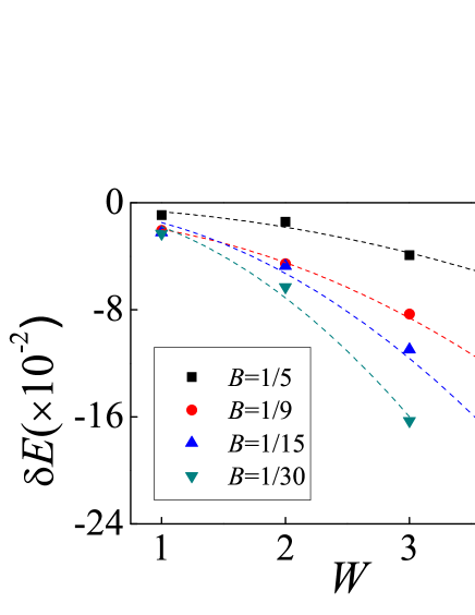
Figure 8: (Color online) Energy deviations between the extended level and the center of the first LB $\delta E\equiv E_{c}(B,W)-\varepsilon_{0}(B)$ are shown as function of disorder $W$. The curves from top to bottom correspond to $B=1/5,\ 1/9,\ 1/15$, and $1/30$. Dashed lines are the fits of quadratic functions $-a(B)W^{2}$. $a(B)$ increases as $B$ decreases.

Figure 9: Phase boundary between the integer QH liquid and the Anderson insulator on $W-1/B$ plane.

Similar anti-levitation is also observed for the extended states in the second lowest LB, but it is less pronounced than that of the lowest LB as commensurate with the principle of level repulsion. The disappearance of the lowest extended state at very small magnetic field indicates a transition between the IQHE state on the lowest LB and an Anderson insulator.

Based on our analysis pertaining to the lowest LB, Fig. 9 displays a phase diagram in the $W-1/B$ plane where the boundary between the integer quantum Hall liquid and Anderson insulator is marked. In principle, the line separating the two phases approaches infinity on the $1/B$ axis as $W\to 0$. It seems to end at $W\approx 7$ on the $W$ axis, implying that no extended state exists beyond this level of disorder. Based on a pertinent experiment,[37], a similar phase diagram is established albeit for higher Landau bands $2<n<10$. Our phase diagram is consistent with the experimental one and extends it to the lowest LB.

IV Conclusions

In this work we numerically studied the behavior of extended state energies $E_{c}(B,W)$ in the lowest LB for an electron on a square lattice with white-noise disorder of strength $W$ subject to an external (perpendicular) magnetic field of strength $B$. It is found that $E_{c}(B,W)$ exhibits disorder- and magnetic-field-driven anti-levitation typically for $W>\hbar\omega_{c}$. Concretely, for fixed magnetic field, $E_{c}(B,W)$ plunges down with the estimate $E_{c}(B,W)-E_{c}(B,0)\sim-a(B)W^{2}$, with $a(B)\sim 1/B$ (at least for weak magnetic field). This scenario may not exist for long-range correlated disorder [31]. The fact that for a fixed disorder strength $W$, $E_{c}(B,W)$ plunges down and eventually disappears as the magnetic field decreases is explained in Ref. 7, based on annihilation of two levels carrying Chern number with opposite signs. A phase diagram of the IQHE is drawn in the $W-1/B$ plane where a clear boundary is identified which distinguishes the IQH liquid and an Anderson insulator.

V Acknowledgement

C. W. thanks T. Ohtsuki for many helpful suggestions concerning the numerical calculations and M. Ma for valuable discussions. Y. A. thanks E. Prodan for discussing the interpretation of his results in Ref. 35. This work is supported by Hong Kong RGC Grants (No. 604109 and No. 605413) and NNSF of China Grant (No. 11374249). The research of Y. A. is partially supported by Israeli Science Foundation Grants No. 1173/2008 and No. 400/2012.

References

- [1] B. Huckestein, Rev. Mod. Phys. 67, 357(1995).
- [2] F. Wegner, Z. Phys. 36, 209(1980).
- [3] The Quantum Hall Effect, edited by R. E. Prange and S. M. Girvin (Springer-Verlag, New York, 1990).
- [4] D. J. Thouless, M. Kohmoto, M. P. Nightingale, and M. den Nijs, Phys. Rev. Lett. 49, 405(1982).
- [5] E. Abrahams, P. W. Anderson, D. C. Licciardello and T. V. Ramakrishnan, Phys. Rev. Lett. 42, 673(1979).
- [6] S. Kivelson, D. H. Lee and S. C. Zhang, Phys. Rev. B 46, 2223(1992).
- [7] D. Z. Liu, X. C. Xie and Q. Niu, Phys. Rev. Lett. 76, 975(1996).
- [8] G. Xiong, S. D. Wang, Q. Niu, D. C. Tian, and X. R. Wang, Phys. Rev. Lett. 87, 216802(2001).
- [9] R. B. Laughlin, Phys. Rev. Lett. 52, 2304(1984).
- [10] D. E. Khmelnitskii, Phys. Lett. 106A, 182(1984).
- [11] F. D. M. Haldane and Kun Yang, Phys. Rev. Lett. 78, 298(1997).
- [12] H. W. Jiang, C. E. Johnson, K. L. Wang, and S. T. Hannahs, Phys. Rev. Lett. 71, 1439(1993).
- [13] T. Wang, K. P. Clark, G. F. Spencer, A. M. Mack, and W. P. Kirk, Phys. Rev. Lett. 72, 709(1994).
- [14] I. Glozman, C. E. Johnson, and H. W. Jiang, Phys. Rev. Lett. 74, 594(1995).
- [15] S. V. Kravchenko, W. Mason, J. E. Furneaux, and V. M. Pudalov, Phys. Rev. Lett. 75, 910(1995).
- [16] D. Shahar, D. C. Tsui, M. Shayegan, R. N. Bhatt, and J. E. Cunningham, Phys. Rev. Lett. 74, 4511(1995).
- [17] D. Shahar, D. C. Tsui, and, J. E. Cunningham, Phys. Rev. B 52, R14372(1995).
- [18] T. V. Shahbazyan and M. E. Raikh, Phys. Rev. Lett. 75, 304(1995).
- [19] V. V. Mkhitaryan, V. Kagalovsky, and M. E. Raikh, Phys. Rev. Lett . 103, 066801 (2009).
- [20] V. V. Mkhitaryan, V. Kagalovsky, and M. E. Raikh, Phys. Rev. B 81, 165426 (2010).
- [21] M. M. Fogler, Phys. Rev. B 57, 11947(1998).
- [22] H. Song, I. Maruyama, and Y. Hatsugai, Phys. Rev. B 76, 132202(2007).
- [23] D. N. Sheng and Z. Y. Weng, Phys. Rev. Lett. 78, 318(1997).
- [24] A. L. C. Pereira and P. A. Schulz, Phys. Rev. B 66, 155323 (2002).
- [25] X. R. Wang, Phys. Rev. B 51, 9310(1995); ibid. 53, 12035(1996).
- [26] X. C. Xie, X. R. Wang and D. Z. Liu, Phys. Rev. Lett. 80, 3563(1998).
- [27] A. Mackinnon and B. Kramer, Z. Phys. B 53, 1(1983).
- [28] D. P. Landau and K. Binder, Phys. Rev. B 31, 5946(1985).
- [29] D. J. Thouless, Phys. Reports 13, 93(1974).
- [30] X. R. Wang, Y. Shapir, and M. Rubinstein, Phys. Rev. A 39, 5974 (1989).
- [31] Th. Koschny, H Potempa, and L. Schweitzer, Phys. Rev. Lett. 86, 3863(2001); Th. Koschny and L. Schweitzer, Phys. Rev. B 70, 165301(2004).
- [32] K. Slevin, T. Ohtsuki, Phys Rev. B 80, 041304(2009).
- [33] Bodo Huckestein and Bernhard Kramer, Phys. Rev. Lett. 64, 1437(1990).
- [34] S.-R. Eric Yang, A. H. MacDonald, B. Huckestein, Phys. Rev. Lett. 74, 3229(1995).
- [35] J. Song and E. Prodan, arXiv:1301.5305v2.
- [36] D. R. Hofstadter, Phys. Rev. B 14, 2239(1976).
- [37] C. F. Huang et al. Phys. Rev. B 65, 045303 (2001).