Tune-out wavelengths for the alkaline earth atoms

Abstract

The lowest 3 tune-out wavelengths of the four alkaline-earth atoms, Be, Mg, Ca and Sr are determined from tabulations of matrix elements produced from large first principles calculations. The tune-out wavelengths are located near the wavelengths for ${}^{3}P^{o}_{1}$ and ${}^{1}P^{o}_{1}$ excitations. The measurement of the tune-out wavelengths could be used to establish a quantitative relationship between the oscillator strength of the transition leading to existence of the tune-out wavelength and the dynamic polarizability of the atom at the tune-out frequency. The longest tune-out wavelengths for Be, Mg, Ca, Sr, Ba and Yb are 454.9813 nm, 457.2372 nm, 657.446 nm, 689.200 nm, 788.875 nm and 553.00 nm respectively.

I Introduction

The dynamic polarizability of an atom gives a measure of the energy shift of the atom when it is exposed to an electromagnetic field Miller and Bederson (1977); Mitroy et al. (2010). For an atom in any given state, one can write

$$\Delta E\approx-\frac{1}{2}\alpha_{d}(\omega)F^{2},$$ (1)

where $\alpha_{d}(\omega)$ is the dipole polarizability of the quantum state at frequency $\omega$, and $F$ is a measure of the strength of the AC electromagnetic field. The limiting value of the dynamic polarizability in the $\omega\to 0$ limit is the static dipole polarizability.

The dynamic polarizability will go to zero for certain frequencies of the applied electromagnetic field. The wavelengths at which the polarizability goes to zero are called the tune-out wavelengths LeBlanc and Thywissen (2007); Arora et al. (2011); Herold et al. (2012); Holmgren et al. (2012); Jiang et al. (2013). Atoms trapped in an optical lattice can be released by changing the wavelength of the trapping laser to that of the tune-out wavelength for that atom. Very recently, tune-out wavelengths have been measured for the rubidium Herold et al. (2012) and the potassium atoms Holmgren et al. (2012). The advantage of a tune-out wavelength measurement is that it is effectively a null experiment, it measures the frequency at which the polarizability is equal to zero. Therefore it does not rely on a precise determination of the strength of an electric field or the intensity of a laser field. Accordingly, it should be possible to measure tune-out wavelengths to high precision and proposals to measure the tune-out wavelengths of some atoms with one or two valence electrons have been advanced Cronin (2013).

The present manuscript describes calculations of the three longest tune-out wavelengths for Be, Mg, Ca and Sr. The tune-out wavelengths for the alkaline-earth atoms arise as a result of the interference between the dynamic polarizability coming from a weak transition and a large background polarizability. The tune-out wavelengths typically occur close to the excitation energy of the weak transitions. The atomic parameters that determine the values of the longest tune-out wavelengths are identified. The calculations utilize tables of matrix elements from earlier calculations of polarizabilities and dispersion coefficients Mitroy (2010); Mitroy and Zhang (2007, 2008a, 2008b, 2010). These were computed using a non-relativistic semi-empirical fixed core approach that has been applied to the description of many one and two electron atoms Mitroy et al. (1988); Mitroy and Bromley (2003a); Mitroy and Safronova (2009); Mitroy et al. (2009). In addition, the longest tune-out wavelengths for Ba and Yb are determined by making recourse to previously determined polarizabilities and oscillator strengths.

II Formulation

The transition arrays for the alkaline earth atoms are essentially those used in previous calculations of the polarizabilities and dispersion coefficients for these atoms Mitroy (2010); Mitroy and Zhang (2007, 2008a, 2008b, 2010). These were computed with a frozen core configuration interaction (CI) method. The Hamiltonian for the two active electrons is written

$$H = \sum_{i=1}^{2}\left(-\frac{1}{2}\nabla^{2}_{i}+V_{\rm dir}({\bf r}_{i})+V_{\rm exc}({\bf r}_{i})+V_{\rm p1}({\bf r}_{i})\right)$$ (2)

$$+ V_{\rm p2}({\bf r}_{1},{\bf r}_{2})+\frac{1}{r_{12}}\ .$$

The direct, $V_{\rm dir}$, and exchange, $V_{\rm exc}$, interactions of the valence electrons with the Hartree-Fock (HF) core were calculated exactly. The $\ell$-dependent polarization potential, $V_{\rm p1}$, was semi-empirical in nature with the functional form

$$V_{\rm p1}({\bf r})=-\sum_{\ell m}\frac{\alpha_{\rm core}g_{\ell}^{2}(r)}{2r^{4}}|\ell m\rangle\langle\ell m|.$$ (3)

The coefficient, $\alpha_{\rm core}$, is the static dipole polarizability of the core and $g_{\ell}^{2}(r)=1-\exp\bigl{(}$-$r^{6}/\rho_{\ell}^{6}\bigr{)}$ is a cutoff function designed to make the polarization potential finite at the origin. The cutoff parameters, $\rho_{\ell}$, were initially tuned to reproduce the binding energies of the corresponding alkaline-earth positive ion, e.g. Mg⁺. Some small adjustments to the $\rho_{\ell}$ were made in the calculations of alkaline-earth atoms to further improve agreement with the experimental spectrum.

A two body polarization term, $V_{p2}$ was also part of the Hamiltonian Hameed (1972); Norcross and Seaton (1976); Mitroy et al. (1988); Mitroy and Bromley (2003a). The polarization of the core by one electron is influenced by the presence of the second valence electron. Omission of the two-body term would typically result in a $ns^{2}$ state that would be too tightly bound. The two body polarization potential is adopted in the present calculation with the form

$$V_{\rm p2}({\bf r}_{i},{\bf r}_{j})=-\frac{\alpha_{\rm core}}{r_{i}^{3}r_{j}^{3}}({\bf r}_{i}\cdot{\bf r}_{j})g_{\rm p2}(r_{i})g_{\rm p2}(r_{j})\ ,$$ (4)

where $g_{p2}$ had the same functional form as $g_{\ell}(r)$. The cutoff parameter for $g_{\rm p2}(r)$ is usually chosen by averaging the different one-electron cutoff parameters.

The use of a fixed core model reduced the calculation of the alkaline-earths and their excited spectra to a two electron calculation. The two electron wavefunctions were expanded in a large basis of two electron configurations formed from a single electron basis mostly consisting of Laguerre Type Orbitals. Typically the total number of one electron states would range from 150 to 200. The use of such large basis sets means that the error due to incompleteness of the basis is typically very small.

Details of the calculations used to represent Be, Mg, Ca and Sr have been previously described Mitroy (2010); Mitroy and Zhang (2007, 2008a, 2008b, 2010). We refer to these semi-empirical models of atomic structure as the configuration interaction plus core polarization (CICP) model in the subsequent text.

For Be, the matrix element list is exactly the same as the matrix element list used in Ref. Mitroy (2010). However, the energies of the low-lying $2s2p\ ^{1,3}P^{o}$ states were set to the experimental binding energies. In the case of the triplet state, the energy chosen was that of the $J=1$ spin-orbit state. Using experimental energies is important for tune-out wavelength calculations since the tune-out wavelength depends sensitively on the precise values of the excitation energies of nearby excited states. In the case of Mg and Ca, the reference matrix elements were those used in dispersion coefficient calculations Mitroy and Zhang (2007, 2008a, 2008b). The energies of the low lying Mg and Ca excited states were also set to experimental values for calculations of the tune-out wavelengths.

The matrix element set for Sr incorporated experimental information. An experimental value was used for the $5s^{2}$ ¹S^e-$5s5p$ ${}^{1}P^{o}$ matrix element Yasuda et al. (2006) and the energy differences for the low-lying excitations were set to the experimental energies. This matrix element set was used to calculate dispersion coefficients between two strontium atoms, and also between strontium and the rare gases Mitroy and Zhang (2010).

Table 1: Theoretical and experimental energy levels (in Hartree) for some of the low-lying states of alkaline-earth metals. The energies are given relative to the energy of the core. The experimental data were taken from the National Institute of Science and Technology (NIST) tabulation Kramida et al. (2012) and for triplet states are the energies of the $J=1$ state.

State	Experiment	CICP
Be
$2s^{2}$ ${}^{1}S^{e}_{0}$	$-$1.0118505	$-$1.0118967
$2s2p$ ${}^{1}P^{o}_{1}$	$-$0.8179085	$-$0.8178898
$2s3p$ ${}^{1}P^{o}_{1}$	$-$0.7376168	$-$0.7376426
$2s2p$ ${}^{3}P^{o}_{1}$	$-$0.9117071	$-$0.9116666
$2s3p$ ${}^{3}P^{o}_{1}$	$-$0.7434484	$-$0.7433848
Mg
$3s^{2}$ ${}^{1}S^{e}_{0}$	$-$0.8335299	$-$0.8335218
$3s3p$ ${}^{1}P^{o}_{1}$	$-$0.6738246	$-$0.6737887
$3s4p$ ${}^{1}P^{o}_{1}$	$-$0.6086897	$-$0.6086551
$3s3p$ ${}^{3}P^{o}_{1}$	$-$0.7338807	$-$0.7336286
$3s4p$ ${}^{3}P^{o}_{1}$	$-$0.6155347	$-$0.6156088
Ca
$4s^{2}$ ${}^{1}S^{e}_{0}$	$-$0.6609319	$-$0.6609124
$4s4p$ ${}^{1}P^{o}_{1}$	$-$0.5531641	$-$0.5531844
$4s5p$ ${}^{1}P^{o}_{1}$	$-$0.4935704	$-$0.4934062
$4s6p$ ${}^{1}P^{o}_{1}$	$-$0.4710284	$-$0.4706060
$4s4p$ ${}^{3}P^{o}_{1}$	$-$0.5916298	$-$0.5913732
$4s5p$ ${}^{3}P^{o}_{1}$	$-$0.4943762	$-$0.4948801
$3d4p$ ${}^{3}P^{o}_{1}$	$-$0.4817070	$-$0.4815337
Sr
$5s^{2}$ ${}^{1}S^{e}_{0}$	$-$0.6146377	$-$0.6146378
$5s5p$ ${}^{1}P^{o}_{1}$	$-$0.5157723	$-$0.5157723
$5s6p$ ${}^{1}P^{o}_{1}$	$-$0.4592740	$-$0.4591686
$5s5p$ ${}^{3}P^{o}_{1}$	$-$0.5485511	$-$0.5476478
$5s6p$ ${}^{3}P^{o}_{1}$	$-$0.4603223	$-$0.4600070
$4d5p$ ${}^{3}P^{o}_{1}$	$-$0.4446740	$-$0.4446176

II.1 Energies

The energy levels of ground state and some of the lowest energy ${}^{1,3}P^{o}$ excited states for Be, Mg, Ca and Sr are listed in Table 1. The polarization potential cutoff parameters were chosen to reproduce the energy of the might most tightly bound state of each symmetry. The energy of the second lowest state does not have to agree with the experimental energy. The reasonable agreement with experimental energies for the second lowest states is an indication that the underlying model Hamiltonian is reliable.

II.2 Line Strengths

Tables 2 and 3 give the line strengths for a number of the low-lying transitions of the alkaline-earth metals comparing with available experimental and theoretical information. The line strength can be calculated as

$$S_{ij}=|\langle\psi_{i};L_{i}J_{i}\parallel\ r^{k}{\bf C}^{k}({\bf\hat{r}})\parallel\psi_{j};L_{j}J_{j}\rangle|^{2}\ .$$ (5)

The CICP values were computed with a modified transition operator Hameed et al. (1968); Hameed (1972); Mitroy et al. (1988), e.g.

$${\bf r}={\bf r}-\left(1-\exp(-r^{6}/\rho^{6})\right)^{1/2}\frac{\alpha_{d}{\bf r}}{r^{3}}.$$ (6)

The cutoff parameter used in Eq. (6) was taken as an average of the $s$, $p$, $d$ and $f$ cutoff parameters. The specific values are detailed elsewhere Mitroy (2010); Mitroy and Zhang (2007, 2008a, 2008b, 2010).

Table 2: Comparison of line strengths for the principal transitions of Be and Mg. The CIDF values are produced using the given oscillator strength and transition energies. The multi-configuration Hartree-Fock (MCHF) and many-body perturbation theory (MBPT) values are derived from the published reduced matrix elements. Numbers in brackets represent the uncertainties in the last digits. The notation $a[b]$ means $a\times 10^{b}$.

Final State	$\Delta E$ (a.u.)	CICP	MCHF	CIDF Glowacki and Migdalek (2006)	MBPT	Experiment
Be
$2s2p$ ${}^{1}P^{o}_{1}$	0.193942	10.63	10.64 Froese Fischer and Tachiev (2004)	10.338	10.63 Porsev and Derevianko (2002)	10.37(39) Reistad and Martinson (1986); 10.36(23) Schnabel and Kock (2000)
$2s3p$ ${}^{1}P^{o}_{1}$	0.274199	0.0474	0.04911 Froese Fischer and Tachiev (2004)
$2s2p$ ${}^{3}P^{o}_{1}$	0.100143		5.947[-8] Froese Fischer and Tachiev (2004)	6.049[-8]
$2s3p$ ${}^{3}P^{o}_{1}$	0.268402		3.182[-9] Froese Fischer and Tachiev (2004)
Mg
$3s3p$ ${}^{1}P^{o}_{1}$	0.159705	16.26	16.05 Froese Fischer et al. (2006)	16.51	16.24 Porsev and Derevianko (2002)	17.56(94) Larsson and Svanberg (1993); 17.22(84) Liljeby et al. (1980); 16.48(81) Kwong et al. (1982)
$3s4p$ ${}^{1}P^{o}_{1}$	0.224840	0.7062	0.7541 Froese Fischer et al. (2006)
$3s3p$ ${}^{3}P^{o}_{1}$	0.099649		3.492[-5] Froese Fischer et al. (2006)	2.806[-5]	4.096[-5] Porsev et al. (2001)	2.78(44)[-5] Godone and Novero (1992); 3.10(42)[-5] Kwong et al. (1982)
$3s4p$ ${}^{3}P^{o}_{1}$	0.217995		4.238[-7] Fischer and Tachiev (2009)

There appears to be no experimental or theoretical data available for the strontium $5s^{2}\ {}^{1}S^{e}\to 5s6p\ ^{3}P^{o}_{1}$ transition Sansonetti and Nave (2010). The line strength adopted for this transition was determined by estimating the mixing between the $5s6p\ ^{1}P^{o}_{1}$ and $5s6p\ ^{3}P^{o}_{1}$ states caused by the spin-orbit interaction. The transition rates for the $5s6p\ ^{1}P^{o}_{1}\to 5s4d\ ^{1}D^{e}_{2}$ and $5s6p\ ^{3}P^{o}_{1}\to 5s4d\ ^{1}D^{e}_{2}$ have been measured Werij et al. (1992); Sansonetti and Nave (2010). The ratio of these transition rates can be used to make an estimate of the singlet:triplet mixing between the two $5s6p$ states with $J=1$. Using the singlet:triplet mixing ratio, and the CICP line strength for the $5s^{2}\ {}^{1}S^{e}\to 5s6p\ ^{1}P^{o}_{1}$ transition, we estimate the $5s^{2}\ {}^{1}S^{e}\to 5s6p\ ^{3}P^{o}_{1}$ line strength to be 0.012.

Table 3: Comparison of line strengths for the principal transitions of Ca, Sr, Ba and Yb. The CIDF line strengths are produced using the given oscillator strength and transition energies. The MCHF and CI+MBPT values are determined from published reduced matrix elements. Numbers in brackets represent the uncertainties in the last digits. The notation $a[b]$ means $a\times 10^{b}$.

Final State	$\Delta E$ (a.u.)	CICP	MCHF	CIDF Glowacki and Migdalek (2003)	MBPT	Experiment
Ca
$4s4p$ ${}^{1}P^{o}_{1}$	0.107768	24.37	24.51 Fischer and Tachiev (2003)		24.31 Porsev and Derevianko (2002)	24.67(90) Zinner et al. (2000); 24.9(4) Kelly and Mathur (1980)
						24.12(1) Vogt et al. (2007); 24.3(1.1) Hansen (1983)
$4s5p$ ${}^{1}P^{o}_{1}$	0.167362	0.00666	0.0529 Fischer and Tachiev (2003)
$4s4p$ ${}^{3}P^{o}_{1}$	0.069302		0.0011022 Fischer and Tachiev (2003)		0.001156 Porsev et al. (2001)	0.00127(3) Husain and Roberts (1986); 0.00124(7) Drozdowski et al. (1997); 0.00127(11) Whitkop and Wiesenfeld (1980)
$4s5p$ ${}^{3}P^{o}_{1}$	0.166556		1.2423[-4] Fischer and Tachiev (2003)
Sr
$5s5p$ ${}^{1}P^{o}_{1}$	0.098865	28.07	32.18 Vaeck et al. (1991)	28.8	28.0 Porsev and Derevianko (2002)	27.54(2) Yasuda et al. (2006); 27.77(16) Nagel et al. (2005);
					27.12 Safronova et al. (2013)	31.0(7) Kelly and Mathur (1980); 29.2(9) Parkinson et al. (1976)
$5s6p$ ${}^{1}P^{o}_{1}$	0.155364	0.0712	0.0492 Vaeck et al. (1991)		0.0790 Safronova et al. (2013)	0.068(10) Parkinson et al. (1976)
$5s5p$ ${}^{3}P^{o}_{1}$	0.066087			0.01718	0.0256 Porsev et al. (2001)	0.02280(54) Yasuda et al. (2006); 0.02206(51) Kelly et al. (1988)
					0.0250 Safronova et al. (2013)	0.02418(50) Husain and Schifino (1984); 0.0213(58) Parkinson et al. (1976)
$5s6p$ ${}^{3}P^{o}_{1}$	0.154315					0.012
Ba
$6s6p$ ${}^{1}P^{o}_{1}$	0.082289			31.8	30.47 Porsev and Derevianko (2002)	29.91(25) Bizzarri and Huber (1990)
					29.92 Dzuba and Ginges (2006)
$6s6p$ ${}^{3}P^{o}_{1}$	0.066087			0.309	0.2746 Dzuba and Ginges (2006)	0.259(13) Miles and Wiese (1969)
Yb
$6s6p$ ${}^{1}P^{o}_{1}$	0.098865			16.9	22.85 Safronova et al. (2012)	17.30 Enomoto et al. (2007) ; 17.206(17) Takasu et al. (2004)
					19.4(7.0) Porsev et al. (1999)
$6s6p$ ${}^{3}P^{o}_{1}$	0.066087			0.324	0.325 Safronova et al. (2012)	0.335 Budick and Snir (1970)
					0.29(8) Porsev et al. (1999)

.

III Polarizabilities

III.1 Static polarizabilities

The polarizabilities for the ground states of Be, Mg, Ca, and Sr are listed in Table 4. All polarizabilities are computed using experimental energy differences for the lowest energy excited states. The present polarizabilities are in good agreement with the previous high quality calculations.

Table 4: Static dipole polarizabilities for the alkaline-earth atom ground states. All values are in atomic units. Hybrid values were computed by replacing the line strength for the resonance transition with the best available experimental value.

	Be	Mg	Ca	Sr
Present: CICP	37.73	71.39	159.4	197.8
Theory: RCCSD Lim et al. (1999)			158.00	198.85
Expt. Molof et al. (1974)			169(17)	186(15)
CI+MBPT Porsev and Derevianko (2006)	37.76	71.33	159.0	202.0
CI+MBPT-SD Safronova et al. (2013)				198.9
Hybrid: Sum rule Porsev and Derevianko (2006)			157.1(1.3)	197.2(2)

. .

These polarizabilities contain contributions from the core electrons. The electric dipole response of the core is described by a pseudo-oscillator strength distribution Margoliash and Meath (1978); Kumar and Meath (1985); Mitroy and Bromley (2003a). Oscillator strength distributions have been constructed by using independent estimates of the core polarizabilities to constrain the sum rules Mitroy and Bromley (2003b, a, 2004); Zhang et al. (2007). These take the form

$$\alpha_{\rm core}=\sum_{i}\frac{f_{i}}{\epsilon_{i}^{2}}$$ (7)

where $f_{i}$ is the pseudo-oscillator strength for a given core orbital and $\epsilon_{i}$ is the excitation energy for that orbital. The sum of the pseudo-oscillator strengths is equal to the number of electrons in the atom. The pseudo-oscillator strength distribution is tabulated in Table 5.

The relative uncertainties in the polarizabilities are assessed at $0.1\%$ for Be, $0.5\%$ for Mg, $1.5\%$ for Ca and $1\%$ for Sr.

Table 5: Pseudo-spectral oscillator strength distributions for the Be²⁺, Mg²⁺, Ca²⁺ and Sr²⁺ cores. Energies are given in a.u.. Refer to the text for interpretation.

$i$	$\varepsilon_{i}$	$f_{i}$	$\varepsilon_{i}$	$f_{i}$
	Be2+		Mg2+
1	10.473672	1.0	50.576100	2.0
2	4.813272	1.0	5.312100	2.0
3			3.826606	6.0
	Ca2+		Sr2+
1	149.495476	2.0	583.696195	2.0
2	16.954485	2.0	80.400045	2.0
3	13.761013	6.0	73.004921	6.0
4	2.377123	2.0	13.484060	2.0
5	1.472453	6.0	10.708942	6.0
6			5.703458	10.0
7			1.906325	2.0
8			1.107643	6.0

III.2 Dynamic polarizabilities and feasibility analysis

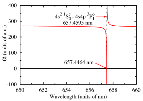
Figure 1: (color online) The dynamic polarizability of the neutral calcium atom in the vicinity of the longest tune-out wavelength.

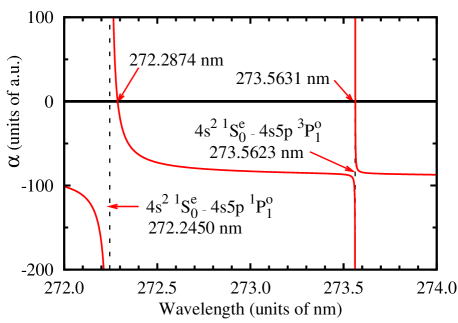
Figure 2: (color online) The dynamic polarizability of the neutral calcium atom in the vicinity of the second and third longest tune-out wavelengths.

The tune-out wavelengths first require calculations of the dynamic polarizabilities. Some non-relativistic forbidden transition to the $nsnp\ ^{3}P^{o}_{1}$ states are included in the present calculation. The line strengths of these transitions are collected from MCHF calculations Fischer and Tachiev (2003); Froese Fischer and Tachiev (2004); Froese Fischer et al. (2006); Fischer and Tachiev (2009) and the all-order MBPT calculations Safronova et al. (2013). These line strengths are listed in Tables 6 and 7.

The dynamic polarizabilities are dominated by the $ns^{2}\ {}^{1}S^{e}$ $\to$ $nsnp\ ^{1}P^{o}_{1}$ resonant transition. Figures 1 and 2 show the dynamic polarizabilities of neutral calcium near the tune-out wavelengths and is typical of all the alkaline-earth atoms. The tune-out wave lengths all occur close to the excitation energies for transitions to ${}^{1}P^{o}_{1}$ or ${}^{3}P^{o}_{1}$ states. The first tune-out wavelength is associated with the $ns^{2}\ {}^{1}S^{e}$ $\to$ $nsnp\ ^{3}P^{o}_{1}$ inter-combination transition. The dynamic polarizability for this transition becomes large and negative just after the photon energy becomes large enough to excite the $nsnp\ ^{3}P^{o}_{1}$ state. This large negative polarizability will cancel with the positive polarizability from the remaining states at the tune-out wavelength. The dynamic polarizability also has a sign change when the photon energy exceeds the excitation energy for the $nsnp\ ^{1}P^{o}_{1}$ state. This change in the polarizability is not associated with a tune-out wavelength. At energies larger than the $ns^{2}\ {}^{1}S^{e}$ $\to$ $nsnp\ ^{1}P^{o}_{1}$ resonant transition energy the polarizability is negative. Additional tune-out wavelengths occur just prior to the excitation energies of the higher $ns^{2}\ {}^{1}S^{e}$ $\to$ ${}^{1,3}P^{o}_{1}$ transitions.

Table 6: Breakdown of contributions to the static polarizability and the dynamic polarizabilities at the three longest tune-out wavelengths, $\lambda_{\rm to}$, for beryllium and magnesium. The remainder term comes from all the valence transitions other than those specifically listed in the Table. The uncertainty in the tune-out wavelength is given by $\delta\lambda_{\rm to}$. The oscillator strength of the transition predominantly cancelling the polarizability due to the resonant transition are given in the row labelled $f$. The notation $a[b]$ means $a\times 10^{b}$.

Be
$\lambda_{\rm to}$ (nm)	$\infty$	454.9813	169.7578	166.422
$\omega_{\rm to}$ (a.u.)	0	0.10014335	0.26840210	0.2737827
$f$		3.970[-9]	5.694[-10]	8.674[-3]
$\delta\lambda_{\rm to}$ (nm)		3.2[-8]	8.2[-10]	0.012
$2s2p$ ${}^{1}P^{o}_{1}$	36.526	49.806	$-$39.908	$-$36.790
$2s3p$ ${}^{1}P^{o}_{1}$	0.115	0.133	2.741	35.093
$2s2p$ ${}^{3}P^{o}_{1}$	0.396[-6]	$-$51.070	$-$0.640[-7]	$-$0.614[-7]
$2s3p$ ${}^{3}P^{o}_{1}$	0.790[-8]	0.918[-8]	35.518	$-$0.195[-6]
Remainder	1.034	1.079	1.597	1.649
$\alpha_{\rm core}$	0.0523	0.0523	0.0524	0.0524
Total	37.728	0	0	0
Mg
$\lambda_{\rm to}$ (nm)	$\infty$	457.2372	209.0108	205.768
$\omega_{\rm to}$ (a.u.)	0	0.09964927	0.21799519	0.2214311
$f$		2.320[-6]	6.159[-8]	0.1056
$\delta\lambda_{\rm to}$ (nm)		0.0002	2.57[-7]	0.238
$3s3p$ ${}^{1}P^{o}_{1}$	67.878	111.151	$-$78.637	$-$73.590
$3s4p$ ${}^{1}P^{o}_{1}$	2.094	2.606	34.922	69.578
$3s3p$ ${}^{3}P^{o}_{1}$	0.234[-3]	$-$115.325	$-$0.617[-4]	$-$0.593[-4]
$3s4p$ ${}^{3}P^{o}_{1}$	0.130[-5]	0.164[-5]	40.017	$-$0.408[-4]
Remainder	0.939	1.086	3.215	3.529
$\alpha_{\rm core}$	0.481	0.482	0.483	0.483
Total	71.392	0	0.0	0

As can be seen from Figure 1 and 2, the tune-out wavelengths for the alkaline-earth atoms arise as a result of the interference between the dynamic polarizability arising from a weak transition and a large background polarizability. In the vicinity of the tune-out wavelength the variation of background polarizability with energy will be much slower than the variation of the tune-out transition. The polarizability near the tune-out wavelength can be modelled as

$$\alpha=\alpha_{0}+\frac{f}{\Delta E^{2}-\omega^{2}}\ ,$$ (8)

where $\alpha_{0}$ is the background polarizability arising from all transitions except the transition near the tune-out wavelength. The background polarizability is evaluated at the tune-out wavelength, $\omega_{\rm to}$. Setting $\alpha=0$ gives

$$\omega_{\rm to}=\sqrt{\Delta E^{2}+\frac{f}{\alpha_{0}}}\ .$$ (9)

When $f/\alpha_{0}<<\Delta E$ is obeyed, and this will generally be the case for the transitions discussed here, one can write

$$\omega_{\rm to}\approx\Delta E\left(1+\frac{f}{2\alpha_{0}\Delta E^{2}}\right)\ .$$ (10)

Equation (10) can be used to make estimate of the tune-out wavelength. When the background polarizability is negative, the tune-out frequency is lower than the excitation energy of the transition triggering the tune-out condition. The quotient, $f/(2\alpha_{0}\Delta E^{2})$ a provides an estimate of the relative difference between the transition frequency and tune-out frequency in the vicinity of a transition.

Equation (10) can also be used for an uncertainty analysis. Setting $X_{\rm shift}=f/(2\alpha_{0}\Delta E^{2})$, one has

$$\frac{\delta X_{\rm shift}}{X_{\rm shift}}=\frac{\delta f}{f}+\frac{\delta\alpha_{0}}{\alpha_{0}}\ .$$ (11)

The contribution to the uncertainty in $X_{\rm shift}$ due to the uncertainty in the transition energy does not have to be considered at the present level of accuracy.

Neglecting the frequency dependence of $\alpha_{0}$, the variation in $\alpha$ with respect to variations in $\omega^{2}$ is

$$\frac{d\alpha}{d\omega^{2}}=\frac{-f}{(\Delta E^{2}-\omega^{2})^{2}}\ .$$ (12)

Writing $\omega^{2}=\omega_{\rm to}^{2}-\delta(\omega^{2})=\Delta E^{2}+\frac{f}{\alpha_{0}}-\delta(\omega^{2})$ in the vicinity of $\omega_{\rm to}$ gives

$$\frac{d\alpha}{d\omega^{2}}=\frac{-f}{\left(\frac{f}{\alpha_{0}}-\delta(\omega^{2})\right)^{2}}\ .$$ (13)

At $\omega=\omega_{\rm to}$, $\delta(\omega^{2})=0$, and one has

$$\frac{d\alpha}{d\omega^{2}}=\frac{-\alpha_{0}^{2}}{f}\ ,$$ (14)

or

$$\frac{d\alpha}{d\omega}=\frac{-2\omega_{0}\alpha_{0}^{2}}{f}\approx\frac{-2\Delta E\alpha_{0}^{2}}{f}\ .$$ (15)

The variation of the polarizability with $\omega$ is inversely proportional to the oscillator strength of the tune-out transition. Let us suppose that the condition for determination of the tune-out wavelength is that the polarizability be set to zero with an uncertainty of $\pm 0.1$ a.u. This means the photon energy should be determined with a frequency uncertainty of

$$\Delta\omega=\frac{0.1f}{2\Delta E\alpha_{0}^{2}}.$$ (16)

For Be and Mg, $\Delta\omega$ would be $7.6\times 10^{-13}$ a.u. and $8.8\times 10^{-11}$ a.u. respectively. These energy widths are very narrow and difficult to achieve with existing technology. The energy windows for calcium and strontium would be $\Delta\omega=5.2\times 10^{-10}$ a.u. and $\Delta\omega=6.9\times 10^{-9}$ a.u. respectively.

III.3 Tune-out wavelengths for Be, Mg, Ca and Sr

Tables 6 and 7 list the three longest tune-out wavelengths for beryllium, magnesium, calcium and strontium. These are determined by explicit calculation of the dynamic polarizability at a series of $\omega$ values. The contributions of the various terms making up the dynamic polarizability at the tune-out wavelengths are given. The longest tune-out wavelength for all the atoms is dominated by two transitions, namely the resonance transition and the longest wavelength inter-combination transition. The size of the polarizability contributions from all other transitions relative to that coming from the resonant transitions are 2.5$\%$, 3.7$\%$, 3.6$\%$ and 3.7$\%$ for Be, Mg, Ca and Sr respectively at the longest tune-out wavelength. This dominant influence of resonant transitions means that a measurement of these tune-out wavelengths will result in a quantitative relationship between the dynamic polarizability and the oscillator strength for the lowest energy inter-combination transition. For example, tune-out wavelengths would make it possible to determine the inter-combination oscillator strength given a value for the polarizability and/or the oscillator strength for the resonance transition.

The differences between the tune-out energy and the nearest excitation energy can be estimated from Eq. (9). Values of $X_{\rm shift}$ for the lowest energy tune-out frequencies for Be $\to$ Sr are $X_{\rm shift}=3.9\times 10^{-9}$, $1.0\times 10^{-6}$, $2.0\times 10^{-5}$ and $3.6\times 10^{-4}$ respectively. These ratios give an initial estimate of the relative precision needed in the wavelength to resolve the tune-out condition. Measurement of the longest tune-out wavelength for beryllium requires a laser with a very precise wavelength. The level of precision required actually exceeds the precision with which the Be $2s^{2}\ {}^{1}S^{e}_{0}\to 2s2p\ ^{3}P^{o}_{1}$ energy is given in the NIST tabulation Kramida et al. (2012). On the other hand, measurement of the Sr tune-out wavelength is much more feasible.

Equation (11) which is used to estimate the uncertainties in $X_{\rm shift}$, can also be used to determine the uncertainties in the tune-out wavelengths. Uncertainties in the tune-out wavelengths are given in Tables 6, 7 and 8.

Table 7: Breakdown of contributions to the static polarizability and dynamic polarizabilities at the three longest tune-out wavelengths for calcium and strontium. The remainder term comes from all the valence transitions other than those specifically listed in the Table. The uncertainty in the tune-out wavelength is given by $\delta\lambda_{\rm to}$. The oscillator strength of the transition predominantly cancelling the polarizability due to the resonant transition are given in the row labelled $f$. The notation $a[b]$ means $a\times 10^{b}$.

Ca
$\lambda_{\rm to}$ (nm)	$\infty$	657.446	273.563	272.287
$\omega_{\rm to}$ (a.u.)	0	0.0693035	0.1665552	0.1673360
$f$		5.092[-5]	1.379[-5]	7.431[-4]
$\delta\lambda_{\rm to}$ (nm)		0.003	0.005	0.282
$4s4p$ ${}^{1}P^{o}_{1}$	150.734	257.030	$-$108.554	$-$106.827
$4s5p$ ${}^{1}P^{o}_{1}$	0.027	0.032	2.760	86.758
$4s6p$ ${}^{1}P^{o}_{1}$	1.097	1.267	4.757	4.911
$4s4p$ ${}^{3}P^{o}_{1}$	0.011	$-$266.414	$-$0.0022	$-$0.0022
$4s5p$ ${}^{3}P^{o}_{1}$	0.497[-3]	0.601[-3]	86.039	$-$0.053
Remainder	4.422	4.919	11.803	12.015
$\alpha_{\rm core}$	3.160	3.166	3.197	3.198
Total	159.452	0	0	0
Sr
$\lambda_{\rm to}$ (nm)	$\infty$	689.200	295.348	293.670
$\omega_{\rm to}$ (a.u.)	0	0.0661105	0.1542699	0.1551514
$f$		1.101[-3]	1.235[-3]	7.371[-3]
$\delta\lambda_{\rm to}$ (nm)		0.042	0.011	0.049
$5s5p$ ${}^{1}P^{o}_{1}$	185.788	336.054	$-$129.482	$-$127.012
$5s6p$ ${}^{1}P^{o}_{1}$	0.305	0.373	21.763	111.764
$4d5p$ ${}^{1}P^{o}_{1}$	0.734	0.848	2.777	2.869
$5s5p$ ${}^{3}P^{o}_{1}$	0.252	$-$348.600	$-$0.057	$-$0.056
$5s6p$ ${}^{3}P^{o}_{1}$	0.052	0.064	87.972	$-$4.772
Remainder	4.901	5.430	11.113	11.292
$\alpha_{\rm core}$	5.813	5.831	5.914	5.915
Total	197.845	0	0	0

Tables 6 and 7 also list the tune-out wavelengths near the $ns(n\!+\!1)\ ^{1,3}P^{o}_{1}$ excitations. These tune-out wavelengths are more sensitive to polarizability contributions from higher transitions. For example, about 25$\%$ of the positive polarizability contributions for the tune-out wavelength associated with the $4s5p\ ^{3}P^{o}_{1}$ excitation come from states other than the $4s^{2}\ {}^{1}S^{e}\to 4s5p\ ^{3}P^{o}_{1}$ transition. These tune-out wavelengths are in the ultra-violet part of the spectrum and would be more difficult to detect in an experiment.

III.4 Heavier systems, Ba and Yb

There are two other atoms, namely, Ba and Yb with similar structures to those discussed earlier. The present calculational methodology cannot be applied to the determination of the tune-out wavelengths for these atoms due to relativistic effects. However, Eq. (9) can be used to make an initial estimate of their longest tune-out wavelengths.

The background polarizability, $\alpha_{0}$ is dominated by the $ns^{2}\ {}^{1}S^{e}_{0}\to nsnp\ ^{1}P^{o}_{1}$ resonant transition which contributes more than $96\%$. The contribution to $\alpha_{0}$ from all other transitions, defined as $\alpha_{\rm rest}$, is much smaller and changes slowly when the frequency changes in the vicinity of the tune-out frequency.

Assuming $\alpha_{\rm rest}$ has the same value at $\omega=0$ and $\omega_{\rm to}$, the value of $\alpha_{\rm rest}$ can be calculated as

$$\alpha_{\rm rest}=\alpha_{d}-\frac{f_{\rm resonant}}{\Delta E_{\rm resonant}^{2}}-\frac{f}{\Delta E^{2}},$$ (17)

where $\alpha_{d}$ is the static polarizability of the ground states, $f_{\rm resonant}$ and $\Delta E_{\rm resonant}$ and $f$ and $\Delta E$ are the oscillator strengths and transition energies of the resonant transition and the transition near the tune-out wavelength respectively. Then the background polarizability $\alpha_{0}$ can be represented as

$$\alpha_{0}=\frac{f_{\rm resonant}}{\Delta E_{\rm resonant}^{2}-\omega^{2}}+\alpha_{\rm rest}.$$ (18)

With this background polarizability, one can approximately predict the tune-out wavelength using Eq. (9).

The differences between the predicted longest tune-out wavelengths in this way and the values obtained using the exact background polarizability are only $2\times 10^{-9}$ nm, $3\times 10^{-6}$ nm, $3\times 10^{-5}$ nm, and $2\times 10^{-3}$ nm for Be $\to$ Sr which are much smaller than the uncertainties of the tune-out wavelengths.

Table 8: Tune-out frequencies, $\omega_{\rm to}$, and wavelengths, $\lambda_{\rm to}$, for the longest tune-out wavelengths of barium and ytterbium. The uncertainty in the tune-out wavelength is given by $\delta\lambda_{\rm to}$. The oscillator strengths and dipole polarizabilities adopted in the calculation are collected from Dzuba and Ginges (2006); Porsev and Derevianko (2006) for barium and Safronova et al. (2012) for ytterbium. The contribution to the polarizability at the tune-out frequency due to the resonance transition is given. The transition energies for barium and Model 2 for ytterbium are taken from the NIST tabulation Kramida et al. (2012). Model 2 for ytterbium has two low-lying strong transitions and data for both are given. The dynamic polarizability of $-$428.162 a.u. for Model 2 for Yb was computed with only the $6s^{2}\ {}^{1}S^{e}_{0}\to 6s6p\ ^{1}P^{o}_{1}$ transition. The second value of $\alpha_{\rm rest}$ allows for the change in the polarizability (due to the $6s6p\ ^{3}P^{o}_{1}$ transition) at the wavelength of 357.78 nm.

Property	Value
Ba
$S_{\rm resonant}$	29.92
$f_{\rm resonant}$	1.641
$\alpha_{d}$ (a.u.)	273.5
$\alpha_{\rm rest}$ (a.u.)	27.92
$f_{\rm resonant}/(\Delta E^{2}_{\rm resonant}-\omega^{2}_{\rm to}$ (a.u.)	477.772
$\Delta E$($6s^{2}\ {}^{1}S^{e}_{0}\to 6s6p\ ^{3}P^{o}_{1}$) (a.u.)	0.05757669
$f$($6s^{2}\ {}^{1}S^{e}_{0}\to 6s6p\ ^{3}P^{o}_{1}$)	0.0105
$\omega_{\rm to}$ (a.u.)	0.0577574
$\lambda_{\rm to}$ (nm)	788.875
$\delta\lambda_{\rm to}$ (nm)	0.295
Yb: Model 1
$S_{\rm resonant}$ (a.u.)	22.85
$f_{\rm resonant}$	1.802
$\alpha_{d}$ (a.u.)	141
$\alpha_{\rm rest}$ (a.u.)	9.614
$f_{\rm resonant}/(\Delta E^{2}_{\rm resonant}-\omega^{2}_{\rm to})$ (a.u.)	249.973
$\Delta E$($6s^{2}\ {}^{1}S^{e}_{0}\to 6s6p\ ^{3}P^{o}_{1}$) (a.u.)	0.08197762
$f$($6s^{2}\ {}^{1}S^{e}_{0}\to 6s6p\ ^{3}P^{o}_{1}$)	0.0178
$\omega_{\rm to}$ (a.u.)	0.0823938
$\lambda_{\rm to}$ (nm)	553.00
Yb: Model 2
$S_{\rm resonant}$ (a.u.)	17.25, 5.543
$f_{\rm resonant}$	1.314, 0.4851
$\alpha_{d}$ (a.u.)	141
$\alpha_{\rm rest}$ (a.u.)	9.614 , 7.726
$\sum_{i}f_{i,\rm resonant}/(\Delta E^{2}_{i,\rm resonant}-\omega^{2}_{\rm to})$ (a.u.)	256.064, $-$426.162
$\Delta E$($6s^{2}\ {}^{1}S^{e}_{0}\to 6s6p\ ^{3}P^{o}_{1}$) (a.u.)	0.08197762
$\Delta E$($6s^{2}\ {}^{1}S^{e}_{0}\to 4f^{-1}6s^{2}5d\ ^{1}P^{o}_{1}$) (a.u.)	0.13148223
$f$($6s^{2}\ {}^{1}S^{e}_{0}\to 6s6p\ ^{3}P^{o}_{1}$)	0.0178
$\omega_{\rm to,1}$ (a.u.)	0.0823844
$\lambda_{\rm to,1}$ (nm)	553.06
$\omega_{\rm to,2}$ (a.u.)	0.126997
$\lambda_{\rm to,2}$ (nm)	358.78

All the information adopted in the calculations for barium and ytterbium are listed in Table 8. The predicted longest tune-out wavelength for barium was $\lambda_{\rm to}=788.875$ nm. The energy window was $\Delta\omega=3.6\times 10^{-8}$ a.u. and $X_{\rm shift}$ was 0.00314. The uncertainty of the longest tune-out wavelengths for barium was $\delta\lambda_{\rm to}=0.295$ nm. The larger uncertainty in this tune-out wavelength was caused by the larger value of $X_{\rm shift}$.

Additional complications are present for ytterbium. The values for Model 1 reported in Table 8 did not explicitly include the nearby $4f^{-1}6s^{2}5d$ ${}^{1}P^{o}_{1}$ state in the polarizability calculation. This spectrum exhibits considerable mixing between the resonance $6s6p$ ${}^{1}P^{o}_{1}$ state and the $4f^{-1}6s^{2}5d$ ${}^{1}P^{o}_{1}$ core excited state Dzuba and Derevianko (2010). This mixing is caused by the small difference in the binding energies for the two states. This is the reason for the large difference between the CI+MBPT and experimental values for the resonant line strength in Table 3. It has been argued that in cases such as this that one should use theoretical energy differences in polarizability calculations Dzuba and Derevianko (2010); Safronova et al. (2012). So for our initial calculation of the tune-out frequency we use the CI+MBPT excitation energy for the resonant transition and the experimental excitation energy for the $6s6p$ ${}^{3}P^{o}_{1}$. This model, which is detailed in Table 7 predicts the longest tune-out wavelengths to be $\lambda_{\rm to}=553.00$ nm. The energy window, $\Delta\omega=1.6\times 10^{-7}$ a.u. while $X_{\rm shift}=0.00509$.

Another model has been made that explicitly includes the $4f^{-1}6s^{2}5d$ ${}^{1}P^{0}_{1}$ state in the polarizability calculation. In this model the line-strength and excitation energy for the resonant excitation energy are set to experimental values. The line strength, 17.25(7), was taken as the average of the two photoassociation line strengths Takasu et al. (2004); Enomoto et al. (2007) and its uncertainty was dervied from the difference of the two values and the quoted uncertainty of Ref. Takasu et al. (2004). The excitation energy for the $4f^{-1}6s^{2}5d$ ${}^{1}P^{o}_{1}$ state is set to experiment. The line strength for the $6s^{2}\ {}^{1}S^{e}_{0}\to 4f^{-1}6s^{2}5d$ ${}^{1}P^{o}_{1}$ transition was tuned by the requiring that the two states of Model 2 have the same polarizability as the resonant excitation for Model 1. A summary of the important parameters of the Model 2 analysis is detailed in Table 8. This model gives a tune-out wavelength of $\lambda_{\rm to}=553.06$ nm. The energy window, $\Delta\omega=1.53\times 10^{-7}$ a.u. while $X_{\rm shift}=0.00497$.

Model 2 also allows for the existence of an additional tune-out wavelength located between the excitation frequencies of the $6s6p$ ${}^{1}P^{0}_{1}$ and $4f^{-1}6s^{2}5d$ ${}^{1}P^{o}_{1}$ states. This tune-out wavelength will be sensitive to the ratio of the respective line strengths and Model 2 predicts $\lambda_{\rm to}=358.78$ nm with $X_{\rm shift}=-0.0332$. For this calculation $\alpha_{\rm rest}$ was set to 7.726 a.u. by allowing for the frequency variation of the polarizability contribution from the $6s^{2}\ {}^{1}S^{e}_{0}\to 6s6p\ ^{3}P^{o}_{1}$ oscillator strength.

The complications of the structure of Yb are so severe that only indicative estimates of the uncertainty are possible. For the longest tune-out frequency, we set $\delta f$, the uncertainty in the $6s^{2}\ {}^{1}S^{e}_{0}\to 6s6p\ ^{3}P^{o}_{1}$ oscillator strength to 1.5$\%$. The uncertainty in the polarizability due to other transitions at the tune-out frequency was initially set to 0.018 Safronova et al. (2012). To this was added an additional uncertainty of $0.024=6/250$, the difference between the Model 1 and 2 predictions of the polarizability at the tune-out frequency. The final uncertainty in the tune-out wavelength of the longest transition was 0.550 nm.

There is little experimental information to assist in the assessment of the uncertainty of the tune-out wavelength near 358.78 nm. The tune-out wavelength lies between the $6s^{2}\ {}^{1}S^{e}_{0}\to 6s6p\ ^{1}P^{o}_{1}$ and $6s^{2}\ {}^{1}S^{e}_{0}\to 4f^{-1}6s^{2}5d\ ^{1}P^{0}_{1}$ transitions and its value would be largely determined by the ratio of the oscillator strengths to those transitions. The uncertainty was determined by an analysis allowing that permitted 1.8$\%$ variations in the polarizability for the two resonant transitions while simultaneously admitting a $0.1/17.25=0.0058$ variation in the $6s^{2}\ {}^{1}S^{e}_{0}\to 6s6p\ ^{1}P^{o}_{1}$ oscillator strength. The uncertainty in $\lambda_{\rm to,2}$ was 0.23 nm. This uncertainty should be interpreted with caution since the value of the tune-out wavelength is very sensitive to line strength adopted for the $6s^{2}\ {}^{1}S^{e}_{0}\to 4f^{-1}6s^{2}5d\ ^{1}P^{0}_{1}$ transition and this is estimated by an indirect method.

IV Conclusion

The three longest tune-out wavelengths for the alkaline-earth atoms from Be to Sr have been estimated from large scale configuration interaction calculations. The longest tune-out wavelengths for Ba and Yb have been estimated by using existing estimates of the polarizability and oscillator strengths. The longest tune-out wavelengths all occur at energies just above the $nsnp$ ${}^{3}P^{o}_{1}$ excitation threshold and arise due to negative polarizability from the $ns^{2}\ {}^{1}S^{e}_{0}\to nsnp\ ^{3}P^{o}_{1}$ inter-combination line cancelling with the rest of the polarizability. The rest of the polarizability is dominated by contributions from the $ns^{2}\ {}^{1}S^{e}_{0}\to nsnp\ ^{1}P^{o}_{1}$ resonant transition, with about 96-97$\%$ of the polarizability arising from this transition. A high precision measurement of the longest tune-out wavelengths is effectively a measure relating the oscillator strength of the $ns^{2}\ {}^{1}S^{e}_{0}\to nsnp\ ^{3}P^{o}_{1}$ inter-combination line to the polarizability of the alkaline-earth atoms. The very small oscillator strengths of the Be and Mg inter-combination lines might make a measurement of the tune-out wavelengths for these atoms difficult. The viability of a tune-out wavelength measurement is greater for the heavier calcium and strontium atoms with their stronger inter-combination lines. The longest wavelengths are all in the visible region.

The second longest tune-out wavelength for all alkaline atoms occurs just before the excitation threshold of the $ns^{2}\ {}^{1}S^{e}_{0}\to ns(n\!+\!1)p\ ^{3}P^{o}_{1}$ transition. Experimental detection of the second longest tune-out wavelength is more difficult since the oscillator strengths of the $ns^{2}\ {}^{1}S^{e}_{0}\to ns(n\!+\!1)p\ ^{3}P^{o}_{1}$ transitions are smaller and the transition is in the ultra-violet. The third longest tune-out wavelengths are typically triggered by the $ns^{2}\ {}^{1}S^{e}_{0}\to ns(n\!+\!1)p\ ^{1}P^{o}_{1}$ transition. The oscillator strengths for the transition are about 0.1-5$\%$ the size of the resonant oscillator strength. The potential for detection of a zero in the dynamic polarizability is larger, but once again the transition lies in the ultraviolet region.