Sampling-Based Temporal Logic Path Planning

Abstract

In this paper, we propose a sampling-based motion planning algorithm that finds an infinite path satisfying a Linear Temporal Logic (LTL) formula over a set of properties satisfied by some regions in a given environment. The algorithm has three main features. First, it is incremental, in the sense that the procedure for finding a satisfying path at each iteration scales only with the number of new samples generated at that iteration. Second, the underlying graph is sparse, which guarantees the low complexity of the overall method. Third, it is probabilistically complete. Examples illustrating the usefulness and the performance of the method are included.

I INTRODUCTION

Motion planning is a fundamental problem that has received a lot of attention from the robotics community [16]. The goal is to generate a feasible path for a robot to move from an initial to a final configuration while avoiding obstacles. Exact solutions to this problem are intractable, and relaxations using potential fields, navigation functions, and cell decompositions are commonly used [5]. These approaches, however, become prohibitively expensive in high dimensional configuration spaces. Sampling-based methods were proposed to overcome this limitation. Examples include the probabilistic roadmap (PRM) algorithm proposed by Kavraki et.al. in [13], which is very useful for multi-query problems, but is not well suited for the integration of differential constraints. In [17], Kuffner and LaValle proposed rapidly-exploring random trees (RRT). RRTs grow randomly, are biased to explore “new” space [17] (Voronoi bias), and find solutions quite fast. Moreover, PRM and RRT were shown to be probabilistically complete [13, 17], but not probabilistically optimal [12]. Karaman and Frazzoli proposed RRT^∗ and PRM^∗, the probabilistically optimal counterparts of RRT and PRM in [12].

Recently, there has been increasing interest in improving the expressivity of motion planning specifications from the classical scenario (“Move from A to B and avoid obstacles.”) to richer languages that allow for Boolean and temporal requirements, e.g., “Visit A, then B, and then C, in this order infinitely often. Always avoid D unless E was visited.” It has been shown that temporal logics, such as Linear Temporal Logic (LTL), Computation Tree Logic (CTL), $\mu$-calculus, and their probabilistic versions (PLTL, PCTL) [1] can be used as formal and expressive specification languages for robot motion [15, 21, 3, 11, 7]. In the above works, adapted model checking algorithms and automata game techniques [15, 4] are used to generate motion plans and control policies for a finite model of robot motion, which is usually obtained through an abstraction process based on partitioning the configuration space [2]. The main limitation of these approaches is their high complexity, as both the synthesis and abstraction algorithms scale at least exponentially with the dimension of the configuration space.

To address this issue, in [11], Karaman and Frazzoli proposed a sampling-based path planning algorithm from specifications given in deterministic $\mu$-calculus. However, deterministic $\mu$-calculus formulae have unnatural syntax based on fixed point operators, and are difficult to use by untrained human operators. In contrast, Linear Temporal Logic (LTL), has very friendly syntax and semantics, which can be easily translated to natural language. One idea would be to translate LTL specifications to deterministic $\mu$-calculus formulae and then proceed with generation of motion plans as in [11]. However, there is no known procedure to transform an LTL formula $\phi$ into a $\mu$-calculus formula $\Psi$ such that the size of $\Psi$ is polynomial in the size of $\phi$ (for details see [6]).

In this paper, we propose a sampling-base path planning algorithm that finds an infinite path satisfying an LTL formula over a set of properties that hold at some regions in the configuration space. The procedure is based on the incremental construction of a transition system followed by the search for one of its satisfying paths. One important feature of the algorithm is that, at a given iteration, it only scales with the number of samples and transitions added to the transitions system at that iteration. This, together with a notion of “sparsity” that we define and enforce on the transition system, play an important role in keeping the overall complexity at a manageable level. In fact, we show that, under some mild assumptions, our definition of sparsity leads to the best possible complexity bound for finding a satisfying path. Finally, while the number of samples increases, the probability that a satisfying path is found approaches 1, i.e., our algorithm is probabilistically complete.

Among the above mentioned papers, the closest to this work is [11]. As in this paper, the authors of [11] can guarantee probabilistic completeness and scalability with added samples only at each iteration of their algorithm. However, in [11], the authors employ the fixed point (Knaster-Tarski) theorem to find a satisfying path. Their method is based on maintaining a “product” graph between the transition system and every sub-formula of their deterministic $\mu$-calculus specification and checking for reachability and the existence of a “type” of cycle on the graph. On the other hand, our algorithm maintains the product automaton between the transition system and a Büchi automaton corresponding to the given LTL specification. Note that, as opposed to LTL model checking [1], we use a modified version of product automaton that ensures reachability of the final states. Moreover, we impose that the states of the transition system be bounded away from each other (by a given function decaying in terms of the size of the transition system). Sparseness is also explored by Dobson and Berkis in [8] for PRM using different techniques.

Our long term goal is to develop a computational framework for automatic deployment of autonomous vehicles from rich, high level specifications that combine static, a priori known information with dynamic, locally sensed events. An example is search and rescue in a disaster relief scenario: an unmanned aircraft is required to keep on photographing some known affected regions and uploading the photos at a known base region. While executing this (global) mission, the aircraft uses its sensors to (locally) identify survivors and fires, with the goal of immediately providing medical assistance to the survivors and extinguishing the fires. The main challenge in this problem is to generate control strategies that guarantee the satisfaction of the global specification in long term while at the same time correctly reacting to locally sensed events. The algorithm proposed in this paper solves the first part of this problem, i.e., the generation of a motion plan satisfying the global specification.

II PRELIMINARIES

For a finite set $\Sigma$, we use $\left|{\Sigma}\right|$ and $2^{\Sigma}$ to denote its cardinality and power set, respectively. $\emptyset$ denotes the empty set.

Definition II.1 (Deterministic Transition System)

A deterministic transition system (DTS) is a tuple $\mathcal{T}=(X,x_{0},\Delta,\Pi,h)$, where:

• $X$ is a finite set of states;

• $x_{0}\in X$ is the initial state;

• $\Delta\subseteq X\times X$ is a set of transitions;

• $\Pi$ is a set of properties (atomic propositions);

• $h:X\rightarrow 2^{\Pi}$ is a labeling function.

We denote a transition $(x,x^{\prime})\in\Delta$ by $x\rightarrow_{\mathcal{T}}x^{\prime}$. A trajectory (or run) of the system is an infinite sequence of states $\mathbf{x}=x_{0}x_{1}\ldots$ such that $x_{k}\rightarrow_{\mathcal{T}}x_{k+1}$ for all $k\geq 0$. A state trajectory $\mathbf{x}$ generates an output trajectory $\mathbf{o}=o_{0}o_{1}\ldots$, where $o_{k}=h(x_{k})$ for all $k\geq 0$. The absence of inputs (control actions) in a DTS implicitly means that a transition $(x,x^{\prime})\in\Delta$ can be chosen deterministically at every state $x$.

A Linear Temporal Logic (LTL) formula over a set of properties (atomic propositions) is defined using standard Boolean operators, $\neg$ (negation), $\wedge$ (conjunction) and $\vee$ (disjunction), and temporal operators, $\mathbf{X}$ (next), $\mathcal{U}$ (until), $\mathbf{F}$ (eventually), $\mathbf{G}$ (always). The semantics of LTL formulae over $\Pi$ are given with respect to infinite words over $2^{\Pi}$, such as the output trajectories of the DTS defined above. Any infinite word satisfying a LTL formula can be written in the form of a finite prefix followed by infinitely many repetitions of a suffix. Verifying whether all output trajectories of a DTS with set of propositions $\Pi$ satisfy an LTL formula over $\Pi$ is called LTL model checking. LTL formulae can be used to describe rich mission specifications. For example, formula $\mathbf{G}(\mathbf{F}(R_{1}\wedge\mathbf{F}R_{2})\wedge\neg O_{1})$ specifies a persistent surveillance task: “visit regions $R_{1}$ and $R_{2}$ infinitely many times and always avoid obstacle $O_{1}$” (see Figure 1). Formal definitions for the LTL syntax, semantics, and model checking can be found in  [1].

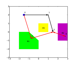
Figure 1: A simple map with three features: an obstacle $O_{1}$ and two regions of interest $R_{1}$ and $R_{2}$. The mission specification is $\phi=\mathbf{G}(\mathbf{F}(R_{1}\wedge\mathbf{F}R_{2})\wedge\neg O_{1})$. The initial position of the robot is marked by the blue disk. The graph (in black and red) represents the generated transition system $\mathcal{T}$. The red arrows specify a satisfying trajectory composed of a prefix $[0,2,3]$ and infinitely many repetitions of the suffix $[4,3,2,3]$.

Definition II.2 (Büchi Automaton)

A (nondeterministic) Büchi automaton is a tuple $\mathcal{B}=(S_{\mathcal{B}},S_{\mathcal{B}_{0}},\Sigma,\delta,F_{\mathcal{B}})$, where:

• $S_{\mathcal{B}}$ is a finite set of states;

• $S_{\mathcal{B}_{0}}\subseteq S_{\mathcal{B}}$ is the set of initial states;

• $\Sigma$ is the input alphabet;

• $\delta:S_{\mathcal{B}}\times\Sigma\rightarrow 2^{S_{\mathcal{B}}}$ is the transition function;

• $F_{\mathcal{B}}\subseteq S_{\mathcal{B}}$ is the set of accepting states.

A transition $(s,s^{\prime})\in\delta(s,\sigma)$ is denoted by $s\stackrel{{\scriptstyle\sigma}}{{\rightarrow}}_{\mathcal{B}}s^{\prime}$. A trajectory of the Büchi automaton $s_{0}s_{1}\ldots$ is generated by an infinite sequence of symbols $\sigma_{0}\sigma_{1}\ldots$ if $s_{0}\in S_{\mathcal{B}_{0}}$ and $s_{k}\stackrel{{\scriptstyle\sigma_{k}}}{{\rightarrow}}s_{k+1}$ for all $k\geq 0$. A input infinite sequence over $\Sigma$ is said to be accepted by a Büchi automaton $\mathcal{B}$ if it generates at least one trajectory of $\mathcal{B}$ that intersects the set $F_{\mathcal{B}}$ of accepting states infinitely many times.

It is shown in [1] that for every LTL formula $\phi$ over $\Pi$ there exists a Büchi automaton $\mathcal{B}$ over alphabet $\Sigma=2^{\Pi}$ such that $\mathcal{B}$ accepts all and only those infinite sequences over $\Pi$ that satisfy $\phi$. There exist efficient algorithms that translate LTL formulae into Büchi automata [9].

Note, that the converse is not true, there are some Büchi automata for which there is no corresponding LTL formulae. However, there are logics such as deterministic $\mu$-calculus which are in 1-to-1 correspondence with the set of languages accepted by Büchi automata.

Model checking a DTS against an LTL formula is based on the construction of the product automaton between the DTS and the Büchi automaton corresponding to the formula. In this paper, we used a modified definition of the product automaton that is optimized for incremental search of a satisfying run. Specifically, the product automaton is defined such that all its states are reachable from the set of initial states.

Definition II.3 (Product Automaton)

Given a DTS $\mathcal{T}=(X,x_{0},\Delta,\Pi,h)$ and a Büchi automaton $\mathcal{B}=(S_{\mathcal{B}},S_{\mathcal{B}_{0}},2^{\Pi},\delta_{\mathcal{B}},F_{\mathcal{B}})$, their product automaton, denoted by $\mathcal{P}=\mathcal{T}\times\mathcal{B}$, is a tuple $\mathcal{P}=(S_{\mathcal{P}},S_{\mathcal{P}_{0}},\Delta_{\mathcal{P}},F_{\mathcal{P}})$ where:

• $S_{\mathcal{P}_{0}}=\{x_{0}\}\times S_{\mathcal{B}_{0}}$ is the set of initial states;

• $S_{\mathcal{P}}\subseteq X\times S_{\mathcal{B}}$ is a finite set of states which are reachable from some initial state: for every $(x^{*},s^{*})\in S_{\mathcal{P}}$ there exists a sequence of $\mathbf{x}=x_{0}x_{1}\ldots x_{n}x^{*}$, with $x_{k}\rightarrow_{\mathcal{T}}x_{k+1}$ for all $0\leq k<n$ and $x_{n}\rightarrow_{\mathcal{T}}x^{*}$, and a sequence $\mathbf{s}=s_{0}s_{1}\ldots s_{n}s^{*}$ such that $s_{0}\in S_{\mathcal{B}_{0}}$, $s_{k}\stackrel{{\scriptstyle h(x_{k})}}{{\rightarrow}}_{\mathcal{B}}s_{k+1}$ for all $0\leq k<n$ and $s_{n}\stackrel{{\scriptstyle h(x_{n})}}{{\rightarrow}}_{\mathcal{T}}s^{*}$;

• $\Delta_{\mathcal{P}}\subseteq S_{\mathcal{P}}\times S_{\mathcal{P}}$ is the set of transitions, defined by: $((x,s),(x^{\prime},s^{\prime}))\in\Delta_{\mathcal{P}}$ iff $x\rightarrow_{\mathcal{T}}x^{\prime}$ and $s\stackrel{{\scriptstyle h(x)}}{{\rightarrow}}_{\mathcal{B}}s^{\prime}$;

• $F_{\mathcal{P}}=(X\times F_{\mathcal{B}})\cap S_{\mathcal{P}}$ is the set of accepting states.

A transition in $\mathcal{P}$ is denoted by $(x,s)\rightarrow_{\mathcal{P}}(x^{\prime},s^{\prime})$ if $((x,s),(x^{\prime},s^{\prime}))\in\Delta_{\mathcal{P}}$. A trajectory $\mathbf{p}=(x_{0},s_{0})(x_{1},s_{1})\ldots$ of $\mathcal{P}$ is an infinite sequence, where $(x_{0},s_{0})\in S_{\mathcal{P}_{0}}$ and $(x_{k},s_{k})\rightarrow_{\mathcal{P}}(x_{k+1},s_{k+1})$ for all $k\geq 0$. Such a trajectory is said to be accepting if and only if it intersects the set of final states $F_{\mathcal{P}}$ infinitely many times. It follows by construction that a trajectory $\mathbf{p}=(x_{0},s_{0})(x_{1},s_{1})\ldots$ of $\mathcal{P}$ is accepting if and only if the trajectory $s_{0}s_{1}\ldots$ is accepting in $\mathcal{B}$. As a result, a trajectory of $\mathcal{T}$ obtained from an accepting trajectory of $\mathcal{P}$ satisfies the given specification encoded by $\mathcal{B}$. For $x\in X$, we define $\beta_{\mathcal{P}}(x)=\{s\in S_{\mathcal{B}}:(x,s)\in S_{\mathcal{P}}\}$ as the set of Büchi states that correspond to $x$ in $\mathcal{P}$. Also, we denote the projection of a trajectory $\mathbf{p}=(x_{0},s_{0})(x_{1},s_{1})\ldots$ onto $\mathcal{T}$ by $\gamma_{\mathcal{T}}(\mathbf{p})=x_{0}x_{1}\ldots$. A similar notation is used for projections of finite trajectories.

For both DTS and automata, we use $\left|{\cdot}\right|$ to denote size, which is the cardinality of the corresponding set of states. A state of a DTS or an automaton is called non-blocking if it has at least one outgoing transition.

III PROBLEM FORMULATION AND APPROACH

Let $\mathcal{D}\subset\mathbb{R}^{n}$ be a compact set denoting the configuration space of a robot. Let $\mathcal{R}$ be a set of disjoint regions in $\mathcal{D}$ and $\Pi$ be a set of properties of interest corresponding to these regions. A map $\sim:\mathcal{R}\rightarrow 2^{\Pi}$ specifies how properties are associated to the regions. Throughout this paper, we will assume that $\mathcal{R}$ is composed of connected sets with non-empty interior, which implies they have non-zero Lebesgue measure (i.e. all regions of interest have full dimension). Also, all connected sets in $\mathcal{D}\setminus\bigcup_{R\in\mathcal{R}}R$ have full dimension. Examples of properties include “obstacle”, “target”, “drop-off”, etc. (see Fig. 1). In practice, the regions and properties are defined in the workspace, and then mapped to the configuration space by using standard techniques [5].

Problem III.1

Given an environment described by $(\mathcal{D},\mathcal{R},\Pi,\sim)$, the initial configuration of the robot $x_{0}\in\mathcal{D}$ and an LTL formula $\phi$ over the set of properties $\Pi$, find a satisfying (infinite) path for the robot originating at $x_{0}$.

A possible approach to Problem III.1 is to construct a partition of the configuration space that contains the regions of interest as elements of the partition. By using input - output linearizations and vector field assignments in the regions of the partition, it was shown that “equivalent” abstractions in the form of finite (not necessarily deterministic) transition systems can be constructed for a large variety of robot dynamics that include car-like vehicles and quadrotors [2, 18, 19]. Model checking and automata game techniques can then be used to control the abstractions from the temporal logic specification [14]. The main limitation of this approach is its high complexity, as both the synthesis and abstraction algorithms scale at least exponentially with the dimension of the configuration space.

In this paper, we propose a sampling-based approach that can be summarized as follows: (1) the LTL formula $\phi$ is translated to the Büchi automaton $\mathcal{B}$; (2) a transition system $\mathcal{T}$ is incrementally constructed from the initial position $x_{0}$ using an RRG-based algorithm; (3) concurrently with (2), the product automaton $\mathcal{P}=\mathcal{T}\times\mathcal{B}$ is updated and used to check if there is a trajectory of $\mathcal{T}$ that satisfies $\phi$. As it will become clear later, our proposed algorithm is probabilistically complete [16, 12] (i.e., it finds a solution with probability 1 if one exists and the number of samples approaches infinity) and the resulting transition system is sparse (i.e., its states are “far” away from each other).

IV PROBLEM SOLUTION

The starting point for our solution to Problem III.1 is the RRG algorithm, which is an extension of RRT [12] that maintains a digraph instead of a tree, and can therefore be used as a model for general $\omega$-regular languages [11]. However, we modify the RRG to obtain a “sparse” transition system that satisfies a given LTL formula. More precisely, a transition system $\mathcal{T}$ is “sparse” if the minimum distance between any two states of $\mathcal{T}$ is greater than a prescribed function dependent only on the size of $\mathcal{T}$ ($\min_{x,x^{\prime}\in\mathcal{T}}\left\|{x-x^{\prime}}\right\|_{2}\geq\eta(\left|{\mathcal{T}}\right|)$). The distance used to define sparsity is inherited from the underlying configuration space and is not related to the graph theoretical distance between states in $\mathcal{T}$. Throughout this paper, we will assume that this distance is Euclidean.

As stated in Section I, sparsity of $\mathcal{T}$ is desired since the solution to Problem III.1 will be the off-line part of a more general procedure that will combine global and local temporal logic specifications. Sparseness also plays an important role in establishing the complexity bounds for the incremental search algorithm (see Section IV-B).

IV-A Sparse RRG

We first briefly introduce the functions used by the algorithm.

Sampling function

The algorithm has access to a sampling function $Sample:\mathbb{N}\rightarrow\mathcal{D}$, which generates independent and identically distributed samples from a given distribution $P$. We assume that the support of $P$ is the entire configuration space $\mathcal{D}$.

Steer function

The steer function $Steer:\mathcal{D}\times\mathcal{D}\rightarrow\mathcal{D}$ is defined based on the robot’s dynamics.  Given a configurations $x$ and goal configuration $x_{g}$, it returns a new configuration $x_{n}$ that can be reached from $x$ by following the dynamics of the robot and that satisfies $\left\|{x_{n}-x_{g}}\right\|_{2}<\left\|{x-x_{g}}\right\|_{2}$.

Near function

$Near:\mathcal{D}\times\mathbb{R}\rightarrow 2^{X}$ is a function of a configuration $x$ and a parameter $\eta$, which returns the set of states from the transition system $\mathcal{T}$ that are at most at $\eta$ distance away from $x$. In other words, $Near$ returns all states in $\mathcal{T}$ that are inside the n-dimensional sphere of center $x$ and radius $\eta$.

Far function

$Far:\mathcal{D}\times\mathbb{R}\times\mathbb{R}\rightarrow 2^{X}$ is a function of a configuration $x$ and two parameters $\eta_{1}$ and $\eta_{2}$. It returns the set of states from the transition system $\mathcal{T}$ that are at most at $\eta_{2}$ distance away from $x$. However, the difference from the $Near$ function is that $Far$ returns an empty set if any state of $\mathcal{T}$ is closer to $x$ than $\eta_{1}$. Geometrically, this means that $Far$ returns a non-empty set for a given state $x$ if there are states in $\mathcal{T}$ which are inside the $n$-dimensional sphere of center $x$ and radius $\eta_{2}$ and all states of $\mathcal{T}$ are outside the sphere with the same center, but radius $\eta_{1}$. Thus, $x$ has to be “far” away from all states in its immediate neighborhood (see Figure 2). This function is used to achieve the “sparseness” of the resulting transition system.

isSimpleSegment function

$isSimpleSegment:\mathcal{D}\times\mathcal{D}\rightarrow\{0,1\}$ is a function that takes two configurations $x_{1}$, $x_{2}$ in $\mathcal{D}$ and returns 1 if the line segment $[x_{1},x_{2}]$ ($\{x\in\mathbb{R}^{n}:x=\lambda x_{1}+(1-\lambda)x_{2},\lambda\in[0,1]\}$) is simple, otherwise it returns 0. A line segment $[x_{1},x_{2}]$ is simple if $[x_{1},x_{2}]\subset\mathcal{D}$ and the number of times $[x_{1},x_{2}]$ crosses the boundary of any region $R\in\mathcal{R}$ is at most one. Therefore, $isSimpleSegment$ returns 1 if either: (1) $x_{1}$ and $x_{2}$ belong to the same region $R$ and $[x_{1},x_{2}]$ does not cross the boundary of $R$ or (2) $x_{1}$ and $x_{2}$ belong to two regions $R_{1}$ and $R_{2}$, respectively, and $[x_{1},x_{2}]$ crosses the common boundary of $R_{1}$ and $R_{2}$ once. $R$ or at most one of $R_{1}$ and $R_{2}$ may be a free space region (a connected set in $\mathcal{D}\setminus\bigcup_{R\in\mathcal{R}}{R}$). See Figure 2 for examples. In Algorithm 1, a transition is rejected if it corresponds to a non-simple line segment (i.e. $isSimpleSegment$ function returns 0). Under this condition, the satisfaction of the mission specification can be checked by only looking at the properties corresponding to the states of the transition system.

Bound functions

$\eta_{1}:\mathbb{Z}_{+}\rightarrow\mathbb{R}$ (lower bound) and $\eta_{2}:\mathbb{Z}_{+}\rightarrow\mathbb{R}$ (upper bound) are functions that define the bounds on the distance between a configuration in $\mathcal{D}$ and the states of the transition system $\mathcal{T}$ in terms of the size of $\mathcal{T}$. These are used as parameters for functions $Far$ and $Near$. We impose $\eta_{1}(k)<\eta_{2}(k)$ for all $k\geq 1$. We also assume that $c\,\eta_{1}(k)>\eta_{2}(k)$, for some finite $c>1$ and all $k\geq 0$. Also, $\eta_{1}$ tends to 0 as $k$ tends to infinity. The rate of decay of $\eta_{1}(\cdot)$ has to be fast enough such that a new sample may be generated. Specifically, the set of all configurations where the center of an $n$-sphere of radius $\eta_{1}/2$ may be placed such that it does not intersect any of the $n$-spheres corresponding to the states in $\mathcal{T}$ has to have non-zero measure with respect to the probability measure $P$ used by the sampling function. One conservative upper bound is $\eta_{1}(k)<\frac{1}{\sqrt{\pi}}\sqrt[n]{\frac{\mu(\mathcal{D})\Gamma(n/2+1)}{k}}$ for all $k\geq 1$, where $\mu(\mathcal{D})$ is the total measure (volume) of the configuration space, $n$ is the dimension of $\mathcal{D}$, and $\Gamma$ is the gamma function. This bound corresponds to the case when there is enough space to insert an $n$-sphere of radius $\eta_{1}/2$ between every two distinct states of $\mathcal{T}$. To simplify the notation, we drop the parameter for these functions and assume that $k$ is always given by the current size of the transition system, $k=\left|{\mathcal{T}}\right|$.

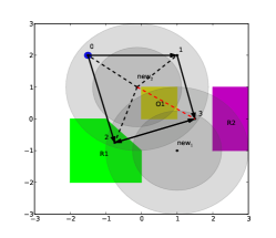
Figure 2: A simple map with three features: an obstacle $O_{1}$ and two regions $R_{1}$, $R_{2}$. The robot is assumed to be a fully actuated point. At the current iteration the states of $\mathcal{T}$ are $\{0,1,2,3\}$. The transitions of $\mathcal{T}$ are represented by the black arrows. The initial configuration is $0$ and is marked by the blue disk. The radii of the dark gray (inner) disks and the light gray (outer) disks are $\eta_{1}$ and $\eta_{2}$, respectively. A new sample $new_{1}\in\mathcal{D}$ is generated, but it will not be considered as a potential new state of $\mathcal{T}$, because it is within $\eta_{1}$ distance from state 3 ($Far(new_{1},\eta_{1},\eta_{2})=\emptyset$). Another sample $new_{2}\in\mathcal{D}$ is generated, which is at least $\eta_{1}$ distance away from all states in $\mathcal{T}$. In this case, $Far(new_{2},\eta_{1},\eta_{2})=\{0,1,2,3\}$ and the algorithm attempts to create transition to and from the new sample $new_{2}$. The transitions $\{(new_{2},0),(0,new_{2}),(new_{2},1),(1,new_{2}),(new_{2},2),(2,new_{2})\}$ (marked by black dashed lines) are added to $\mathcal{T}$, because all these transitions correspond to simple line segments ($isSimpleSegment$ returns 1 for all of them). For example, $isSimpleSegment(new_{2},0)=1$, because $new_{2}$ and $0$ belong to the same region (the free space region) and $[new_{2},0]$ does not intersect any other region. $isSimpleSegment(new_{2},2)=1$, because $[new_{2},2]$ crosses the boundary between the free space region and region $R_{1}$ once. On the other hand, the transitions $\{(new_{2},3),(3,new_{2})\}$ (marked by red dashed lines) are not added to $\mathcal{T}$, since they pass over the obstacle $O_{1}$. In this case, $isSimpleSegment(3,new_{2})=0$, because $3$ and $new_{2}$ are in the same region, but $[3,new_{2}]$ crosses the boundary of $O_{1}$ twice.

The goal of the modified RRG algorithm (see Algorithm 1) is to find a satisfying run, but such that the resulting transition system is “sparse”, i.e. states are “sufficiently” apart from each other. The algorithm iterates until a satisfying run originating in $x_{0}$ is found.

At each iteration, a new sample $x_{r}$ is generated (line 6 in Algorithm 1). For each state $x$ in $\mathcal{T}$ which is “far” from the sample $x_{r}$ ($x\in Far(x_{r},\eta_{1},\eta_{2})$), a new configuration $x^{\prime}_{r}$ is computed such that the robot can be steered from $x$ to $x^{\prime}_{r}$ and the distance to $x_{r}$ is decreased (line 10). The two loops of the algorithm (lines 7–13 and 16–21) are executed if and only if the $Far$ function returns a non-empty set. However, $x^{\prime}_{r}$ is regarded as a potential new state of $\mathcal{T}$, and not $x_{r}$. Thus, the $Steer$ function plays an important role in the “sparsity” of the final transition system. Next, it is checked if the potential new transition $(x,x^{\prime}_{r})$ is a simple segment (line 9). It is also verified if $x^{\prime}_{r}$ may lead to a solution, which is equivalent to testing if $x^{\prime}_{r}$ induces at least one non-blocking state in $\mathcal{P}$ (see Algorithm 2). If configuration $x^{\prime}_{r}$ and the corresponding transition $(x,x^{\prime}_{r})$ pass all tests, then they are added to the list of new states and list of new transitions of $\mathcal{T}$, respectively (lines 12–13).

After all “far” neighbors of $x_{r}$ are processed, the transition system is updated. Note that at this point $\mathcal{T}$ was only extended with states that explore “new space”. However, in order to model $\omega$-regular languages the algorithm must also close cycles. Therefore, the same procedure as before (lines 7–14) is also applied to the newly added states $X^{\prime}$ (lines 15–21 of Algorithm 1). The difference is that it is checked if states from $X^{\prime}$ can steer the robot back to states in $\mathcal{T}$ in order to close cycles. Also, because we know that the states in $X^{\prime}$ are “far” from their neighbors, the $Near$ function will be used instead of the $Far$ function. The algorithm returns a (prefix, suffix) pair in $\mathcal{T}$ obtained by projection from the corresponding path ($p_{0}\stackrel{{\scriptstyle*}}{{\rightarrow}}p_{F}$) and cycle ($p_{F}\stackrel{{\scriptstyle+}}{{\rightarrow}}p_{F}$) in $\mathcal{P}$, respectively. The $*$ above the transition symbol means that the length of the path can be 0, while $+$ denotes that the length of the cycle must be at least 1.

Input: $\mathcal{B}$ – Büchi automaton corresponding to $\phi$

Input: $x_{0}$ initial configuration of the robot

Output: (prefix, suffix) in $\mathcal{T}$

1

2Construct $\mathcal{T}$ with $x_{0}$ as initial state

3 Construct $\mathcal{P}=\mathcal{T}\times\mathcal{B}$

4 Initialize $scc(\cdot)$

5

6while $\neg(x_{0}\models\phi)$ $(\equiv\neg(\exists p\in F_{\mathcal{P}}$ s.t. $\left|{scc(p)}\right|>1))$ do

7       $X^{\prime}\leftarrow\emptyset$, $\Delta^{\prime}\leftarrow\emptyset$, $\Delta^{\prime}_{\mathcal{P}}\leftarrow\emptyset$

8       $x_{r}\leftarrow Sample()$

9       foreach $x\in Far(x_{r},\eta_{1},\eta_{2})$ do

10             $x^{\prime}_{r}\leftarrow Steer(x,x_{r})$

11             if $isSimpleSegment(x_{r},x^{\prime}_{r})$ then

12                   $added\leftarrow updatePA(\mathcal{P},\mathcal{B},(x,x^{\prime}_{r}))$

13                   if $added$ is True then

14                         $X^{\prime}\leftarrow X^{\prime}\cup\{x^{\prime}_{r}\}$

15                         $\Delta^{\prime}\leftarrow\Delta^{\prime}\cup\{(x,x^{\prime}_{r})\}$

16                        

17                  

18            

19      $\mathcal{T}\leftarrow\mathcal{T}\cup(X^{\prime},\Delta^{\prime})$

20      

21      $\Delta^{\prime}\leftarrow\emptyset$, $\Delta^{\prime}_{\mathcal{P}}\leftarrow\emptyset$

22       foreach $x^{\prime}_{r}\in X^{\prime}$ do

23             foreach $x\in Near(x^{\prime}_{r},\eta_{2})$ do

24                   if $(x=Steer(x^{\prime}_{r},x))\wedge isSimpleSegment(x^{\prime}_{r},x)$ then

25                         $added\leftarrow updatePA(\mathcal{P},\mathcal{B},(x,x^{\prime}_{r}))$

26                         if $added$ is True then

27                               $\Delta^{\prime}\leftarrow\Delta^{\prime}\cup\{(x^{\prime}_{r},x)\}$

28                              

29                        

30                  

31            

32      $\mathcal{T}\leftarrow\mathcal{T}\cup(X^{\prime},\Delta^{\prime})$

33      

return $(\gamma_{\mathcal{T}}(p_{0}\stackrel{{\scriptstyle*}}{{\rightarrow}}p_{F}),\gamma_{\mathcal{T}}(p_{F}\stackrel{{\scriptstyle+}}{{\rightarrow}}p_{F}))$, where $p_{F}\in F_{\mathcal{P}}$

Algorithm 1 Sparse RRG

In the end, the result is a transition system $\mathcal{T}$ which captures the general topology of the environment. In the next section, we will show that $\mathcal{T}$ also yields a run that satisfies the given specification.

IV-B Incremental search for a satisfying run

The proposed approach of incrementally constructing a transition system raises the problem of how to efficiently check for a satisfying run at each iteration. As mentioned in the previous section, the search for satisfying runs is performed on the product automaton. Note that testing whether there exists a trajectory of $\mathcal{T}$ from the initial position $x_{0}$ that satisfies the given LTL formula $\phi$ is equivalent to searching for a path from an initial state $p_{0}$ to a final state $p_{F}$ in the product automaton $\mathcal{P}=\mathcal{T}\times\mathcal{B}$ and for a cycle containing $p_{F}$ of length greater than 1, where $\mathcal{B}$ is the Büchi automaton corresponding to $\phi$. If such a path and a cycle are found then their projection onto $\mathcal{T}$ represents a satisfying infinite trajectory (line 23 of Algorithm 1). Testing whether $p_{F}$ belongs to a non-degenerate cycle (length greater than 1) is equivalent to testing if $p_{F}$ belong to a non-trivial strongly connected component – SCC (the size of the SCC is greater than 1). Checking for a satisfying trajectory in $\mathcal{P}$ is performed incrementally as the transition system is modified.

The reachability of the final states from initial ones in $\mathcal{P}$ is guaranteed by construction (see Definition II.3). However, we need to define a procedure (see Algorithm 2) to incrementally update $\mathcal{P}$ when a new transition is added to $\mathcal{T}$. Consider the (non-incremental) case of constructing $\mathcal{P}=\mathcal{T}\times\mathcal{B}$. This is done by a traversal of $\bar{\mathcal{P}}=(X\times S_{\mathcal{B}},\bar{\Delta}_{\mathcal{P}})$ from all initial states, where $((x,s),(x^{\prime},s^{\prime}))\in\bar{\Delta}_{\mathcal{P}}$ if $p\rightarrow p^{\prime}$ and $s\stackrel{{\scriptstyle h(x)}}{{\rightarrow}}s^{\prime}$. $\bar{\mathcal{P}}$ is a product automaton but without the reachability requirement. This suggests that the way to update $\mathcal{P}$ when a transition $(x,x^{\prime})$ is added to $\mathcal{T}$, is to do a traversal from all states $p$ of $\mathcal{P}$ such that $\gamma_{\mathcal{T}}(p)=x$. Also, it is checked if $x^{\prime}$ induces any non-blocking states in $\mathcal{P}$ (lines 1-3 of Algorithm 2). The test is performed by computing the set $S^{\prime}_{\mathcal{P}}$ of non-blocking states of $\mathcal{P}$ (line 1) such that $p^{\prime}\in S^{\prime}_{\mathcal{P}}$ has $\gamma_{\mathcal{T}}(p^{\prime})=x^{\prime}$ and $p^{\prime}$ is obtained by a transition from $\{(x,s):s\in\beta_{\mathcal{P}}(x)\}$. If $S^{\prime}_{\mathcal{P}}$ is empty then the transition $(x,x^{\prime})$ of $\mathcal{T}$ is discarded and the procedure stops (line 3). Otherwise, the product automaton $\mathcal{P}$ is updated recursively to add all states that become reachable because of the states in $S^{\prime}_{\mathcal{P}}$. The recursive procedure is performed from each state in $S^{\prime}_{\mathcal{P}}$ as follows: if a state $p$ (line 7) is not in $\mathcal{P}$, then it is added to $\mathcal{P}$ together with all its outgoing transitions (line 10) and the recursive procedure continues from the outgoing states of $p$; if $p$ is in $\mathcal{P}$ then the traversal stops, but its outgoing transitions are still added to $\mathcal{P}$ (line 14). The incremental construction of $\mathcal{P}$ has the same overall complexity as constructing $\mathcal{P}$ from the final $\mathcal{T}$ and $\mathcal{B}$, because the recursive procedure just performes traversals that do not visit states already in $\mathcal{P}$. Thus, we focus our complexity analysis on the next step of the incremental search algorithm.

Input: $\mathcal{P}$ – product automaton

Input: $\mathcal{B}$ – Büchi automaton

Input: $(x,x^{\prime})$ – new transition in $\mathcal{T}$

Output: Boolean value – indicates if $\mathcal{P}$ was modified

1

2$S^{\prime}_{\mathcal{P}}\leftarrow\{(x^{\prime},s^{\prime}):s\stackrel{{\scriptstyle h(x)}}{{\rightarrow}}_{\mathcal{B}}s^{\prime},s\in\beta_{\mathcal{P}}(x),s^{\prime}$ non-blocking$\}$

3 $\Delta^{\prime}_{\mathcal{P}}\leftarrow\{((x,s),(x^{\prime},s^{\prime})):s\in\beta_{\mathcal{P}}(x),s\stackrel{{\scriptstyle h(x)}}{{\rightarrow}}_{\mathcal{B}}s^{\prime},\ (x^{\prime},s^{\prime})\in S^{\prime}_{\mathcal{P}}\}$

4 if $S^{\prime}_{\mathcal{P}}\neq\emptyset$ then

5       $\mathcal{P}\leftarrow\mathcal{P}\cup(S^{\prime}_{\mathcal{P}},\Delta^{\prime}_{\mathcal{P}})$

6       $stack\leftarrow S^{\prime}_{\mathcal{P}}$

7       while $stack\neq\emptyset$ do

8             $p_{1}=(x_{1},s_{1})\leftarrow stack.pop()$

9             foreach $p_{2}\in\{(x_{2},s_{2}):x_{1}\rightarrow_{\mathcal{T}}x_{2},s_{1}\stackrel{{\scriptstyle h(x_{1})}}{{\rightarrow}}_{\mathcal{B}}s_{2}\}$ do

10                   if $p_{2}\notin S_{\mathcal{P}}$ then

11                         $\mathcal{P}\leftarrow\mathcal{P}\cup(\{p_{2}\},\{(p_{1},p_{2})\})$

12                         $\Delta^{\prime}_{\mathcal{P}}\leftarrow\Delta^{\prime}_{\mathcal{P}}\cup\{(p_{1},p_{2})\}$

13                         $stack\leftarrow stack\cup\{p_{2}\}$

14                        

15                  else if $(p_{1},p_{2})\notin\Delta_{\mathcal{P}}$ then

16                         $\Delta_{\mathcal{P}}\leftarrow\Delta_{\mathcal{P}}\cup\{(p_{1},p_{2})\}$

17                         $\Delta^{\prime}_{\mathcal{P}}\leftarrow\Delta^{\prime}_{\mathcal{P}}\cup\{(p_{1},p_{2})\}$

18                        

19                  

20            

21      updateSCC($\mathcal{P}$, $scc$, $\Delta^{\prime}_{\mathcal{P}}$)

22       return True

return False

Algorithm 2 Incremental Search for a Satisfying Run

The second part of the incremental search procedure is concerned with maintaining the strongly connected components (SCCs) of $\mathcal{P}$ (line 14 of Algorithm 2) as new transitions are added (these are stored in $\Delta^{\prime}_{\mathcal{P}}$ in Algorithm 2). To incrementally maintain the SCCs of the product automaton, we employ the soft-threshold-search algorithm presented in [10]. The algorithm maintains a topological order of the super-vertices corresponding to each SCC. When a new transition is added to $\mathcal{P}$, the algorithm proceeds to re-establish a topological order and merges vertices if new SCCs are formed. The details of the algorithm are presented in [10]. The authors also offer insight about the complexity of the algorithm. They show that, under a mild assumption, the incremental algorithm has the best possible complexity bound.

Incrementally maintaining $\mathcal{P}$ and its SCCs yields a quick way to check if a trajectory of $\mathcal{T}$ satisfies $\phi$ (line 4 of Algorithm 1). The next theorem establishes the overall complexity of Algorithm 2.

Theorem IV.1

The execution time of the incremental search algorithm 2 is $O(m^{\frac{3}{2}})$, where $m$ is the number of transitions added to $\mathcal{T}$ in Algorithm 1.

Remark IV.2

First, note that the execution time of the incremental procedure is better by a polynomial factor than naively running a linear-time SCC algorithm at each step, since this will have complexity $O(m^{2})$. The algorithm presented in [10] improves the previously best known bound by a logarithmic factor (for sparse graphs). The proof exploits the fact that the “sparseness” (metric) property we defined implies a topological sparseness, i.e., $\mathcal{T}$ is a sparse graph.

Proof:

The proof of the theorem is based on the analysis from [10] of incremental SCC algorithms. Haeupler et.al. show that any incremental algorithm that satisfies a “local” property must take at least $\Omega(n\sqrt{m})$ time, where $n$ is the number of nodes in the graph and $m$ is the number of edges. The “local” property is a mild assumption that restricts the algorithm to reorder only vertices that are affected by the addition of an edge. This implies that the incremental SCC algorithm has the best possible complexity bound, in asymptotic sense, if and only if the graph is sparse. A graph is sparse if the the number of edges is asymptotically the same as the number of nodes, i.e. $m=O(n)$. What we need to show is that the transition system generated by Algorithm 1 is sparse. Note that although we run the SCC algorithm on the product automaton, the asymptotic execution time is not affected by analyzing the transition system instead of the product automaton, because the Büchi automaton is fixed. This follows from $\left|{S_{\mathcal{P}}}\right|\leq\left|{S_{\mathcal{B}}}\right|\cdot\left|{X}\right|$ and $\left|{\Delta_{\mathcal{P}}}\right|\leq\left|{\delta_{\mathcal{B}}}\right|\cdot\left|{\Delta}\right|$.

Intuitively, the underlying graph of $\mathcal{T}$ is sparse, because the states were generated “far” from each other. When a new state is added to $\mathcal{T}$, it will be connected to other states that are at least $\eta_{1}$ and at most $\eta_{2}$ distance away. Also, all states in $\mathcal{T}$ are at least $\eta_{1}$ distance away from each other. This implies that there is a bound on the density of states. This bound is related to the kissing number [20]. The kissing number is the maximum number of non-overlapping spheres that touch another given sphere. Using this intuition, the problem of estimating the maximum number of neighbors of a state can be restated as a sphere packing problem. Given a state $x$, each neighbor can be thought of as a sphere with radius $\eta_{1}/2$ and center belonging to the volume delimited by two spheres centered at $x$ and with radii $\eta_{1}$ and $\eta_{2}$, respectively. Since, $\eta_{1}<\eta_{2}<c\eta_{1}$ for some $c>1$ it follows, that there will be only a finite number of spheres which can be placed inside the described volume. Thus there is a finite bound on the number of neighbors a state can have, which depends only on the dimension and shape of the configuration space and the volume between two concentric spheres of radii $\eta_{1}$ and $\eta_{2}$, respectively. ∎

Remarks IV.3

The bound on the number of neighbors can become very large as the dimension of the configuration space increases.

As we have seen in the proof, under the “local” property assumption, the incremental search algorithm has the best possible complexity bound. Because we do the search for a satisfying run using a Büchi automaton, through the product automaton, and not the LTL formula directly, the proposed method is general enough to be applied in conjunction with logics (such as $\mu$-calculus), which are as expressive as the languages accepted by Büchi automata. Also, we do not expect to obtain search algorithms that are asymptotically faster then the proposed one (for sparse graphs), since this would violate the lower bound obtained in [10] (assuming the “local” property).

IV-C Probabilistic completeness

The presented RRG-based algorithm retains the probabilistic completeness of RRT, since the constructed transition system is composed of an RRT-like tree and some transitions which close cycles.

Theorem IV.4

Algorithm 1 is probabilistically complete.

Proof:

(Sketch) First we start by noting that any word in a $\omega$-regular language can be represented by a finite prefix and a finite suffix, which is repeated indefinitely [1]. This is important, since this shows that a solution, represented by a transition system, is completely characterized by a finite number of states. Let us denote by $\bar{X}$ the finite set of states that define a solution. It follows from the way regions are defined that we can choose a neighborhood around each state in $\bar{X}$ such that the system can be steered in one step from all points in one neighborhood to all points in the next neighborhood. Thus, we can use induction to show that [KF-ACC12]: (1) there is a non-zero probability that a sample will be generated inside the neighborhood of the first state in the solution sequence; (2) if there is a state in $\mathcal{T}$ that is inside the neighborhood of the $k$-th state from the solution sequence, then there is a non-zero probability that a sample will be generated inside the $k+1$-st state’s neighborhood. Therefore, as the number of samples goes to infinity, the probability that the transition system $\mathcal{T}$ has nodes belonging to all neighborhoods of states in $\bar{X}$ goes to 1. To finish the proof, note that we have to show that the algorithm is always able to generate samples with the desired “sparseness” property. However, recall that the bound functions must converge to 0 (as the number of states goes to infinity) fast enough such that the set of configurations for which “Far” function returns a non-empty list has non-zero measure with respect to the sampling distribution. This concludes the proof. ∎

V IMPLEMENTATION AND CASE STUDIES

We implemented the algorithms presented in this paper in Python2.7. In this section, we present some examples in configuration spaces of dimensions 2, 10 and 20. In all cases, we assume for simplicity that the $Steer$ function is trivial, i.e., there are no actuation constraints at any given configuration. All examples were ran on an iMac system with a 3.4 GHz Intel Core i7 processor and 16GB of memory.

Case Study 1: Consider the configuration space depicted in Figure 3. The initial configuration is at $(0.3;0.3)$. The specification is to visit regions $r1$, $r2$, $r3$ and $r4$ infinitely many times while avoiding regions $o1$, $o2$, $o3$ and $o4$. The corresponding LTL formula for the given mission specification is

$$\phi_{1} = \mathbf{G}(\mathbf{F}r1\wedge(\mathbf{F}r2\wedge(\mathbf{F}r3\wedge(\mathbf{F}r4)))$$

$$\wedge\neg(o1\vee o2\vee o3\vee o4))$$

A solution to this problem is shown in Figures 3 and 4. We ran the overall algorithm 20 times and obtained an average execution time of 6.954 sec, out of which the average of the incremental search algorithm was 6.438 sec. The resulting transition system had a mean size of 51 states and 277 transitions, while the corresponding product automaton had a mean size of 643 states and 7414 transitions. The Büchi automaton corresponding to $\phi_{1}$ had 20 states and 155 transitions.

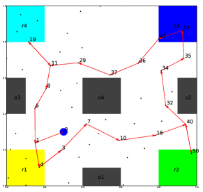
Figure 3: One of the solutions corresponding to Case Study 1: the specification is to visit all the colored regions labelled $r1$ (yellow), $r2$ (green), $r3$ (blue) and $r4$ (cyan) infinitely often, while avoiding the dark gray obstacles labelled $o1$, $o2$, $o3$, $o4$. The black dots represent the states of the transition system $\mathcal{T}$ (51 states and 264 transitions). The starting configuration of the robot (the initial state of $\mathcal{T}$) is denoted by the blue circle. The red arrows represent the satisfying run (finite prefix, suffix pair) found by Algorithm 1, which is composed of 21 states from $\mathcal{T}$. In this case, the prefix and suffix are [0, 1, 4, 3] and [7, 10, 16, 40, 50, 40, 32, 34, 35, 43, 47, 36, 37, 29, 11, 19, 11, 8, 5, 1, 4, 3], respectively.

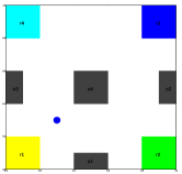
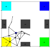
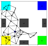
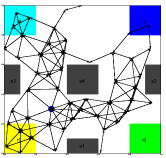
Figure 4: Transition systems obtained at earlier iterations corresponding to the solution shown in Figure 3 (to be read from left to right and top to bottom). The black dots and arrows represent the state and transitions of $\mathcal{T}$, respectively.

Case Study 2: Consider a 10-dimensional unit hypercube configuration space. The specification is to visit regions $r1$, $r2$, $r3$ infinitely many times, while avoiding region $o1$. The LTL formula corresponding to this specification is

$$\phi_{2}=\mathbf{G}(\mathbf{F}r1\wedge(\mathbf{F}r2\wedge(\mathbf{F}r3))\wedge\neg o1).$$ (2)

The corresponding Büchi automaton has 9 states and 43 transitions. Regions $r1=[0;0.4]\times[0;0.75]^{9}$, $r2=[0.6;1]\times[0.25;1]^{9}$, $r3=[0.6;1]\times[0;0.2]\times([0.2;1]\times[0;0.8])^{4}$ and $o1=[0.41;59]\times[0.3;0.9]\times[0.12;0.88]^{8}$ are hypercubes and their volumes are 0.03, 0.03, 0.013 and 0.012, respectively. $r1$, $r2$, $r3$ are positioned in the corners of the configuration space, while $o1$ is positioned in the center. In this case, the algorithm took 16.75 sec on average (20 experiments), while just the incremental search procedure for a satisfying run took 14.471 sec. The transition system had a mean size of 69 states and 1578 transitions, while the product automaton had a mean size of 439 states and 21300 transitions.

Case Study 3: We also considered a 20-dimensional unit hypercube configuration space. Two hypercube regions $r1$ and $r2$ were defined and the robot was required to visit both of them infinitely many times ($\phi_{3}=\mathbf{G}(\mathbf{F}(r1\wedge\mathbf{F}r2))$). The overall algorithm took 7.45 minutes, while the transition system grew to 414 states and 75584 transitions. The corresponding product automaton had a size of 1145 states and 425544 transitions. This example illustrates the fact that the bound on the number of neighbors of a state in the transition system grows at least exponentially in the dimension of the configuration space.

The performed tests suggest some possible practical improvements of the execution time of the proposed algorithms. One idea is to postpone the incremental maintenance of SCCs until there is at least one final state in $\mathcal{P}$. We are interested in SCCs only for final states anyway, therefore there is no benefit to compute them before final states are found. A linear-time SCC algorithm can be used to initialize the corresponding incremental SCC structure when final states are found. Another important improvement may be obtained by processing transitions of $\mathcal{P}$ in batches. At each iteration, multiple transitions are added simultaneously, thus a batch version of the incremental SCC may greatly reduce the total execution time. Note that these heuristics will not improve the asymptotic bound of the algorithm. Also, the size of the Büchi automaton has a significant impact on execution time of the procedure, even though it is fixed and does not contribute to the overall asymptotic bound.

VI FUTURE WORK

As already suggested, future work will include integrating the presented algorithm with a local on-line sensing and planning procedure. The overall framework will ensure correctness with respect to both global and local temporal logic specifications. We will also incorporate realistic robot dynamics and environment topologies and we will perform experimental validations with air and ground vehicles in our lab.

References

- [1] Christel Baier and Joost-Pieter Katoen. Principles of model checking. MIT Press, 2008.
- [2] C. Belta, V. Isler, and G. J. Pappas. Discrete abstractions for robot planning and control in polygonal environments. IEEE Trans. on Robotics, 21(5):864–874, 2005.
- [3] A. Bhatia, L.E. Kavraki, and M.Y. Vardi. Sampling-based motion planning with temporal goals. In Robotics and Automation (ICRA), IEEE International Conference on, pages 2689–2696. IEEE, 2010.
- [4] Yushan Chen, Jana Tumova, and Calin Belta. LTL Robot Motion Control based on Automata Learning of Environmental Dynamics. In IEEE International Conference on Robotics and Automation (ICRA), Saint Paul, MN, USA, 2012.
- [5] H. Choset, K.M. Lynch, S. Hutchinson, G. Kantor, W. Burgard, L.E. Kavraki, and S. Thrun. Principles of Robot Motion: Theory, Algorithms, and Implementations. MIT Press, Boston, MA, 2005.
- [6] S. Cranen, J.F. Groote, and M.A. Reniers. A linear translation from LTL to the first-order modal -calculus. Technical Report 10-09, Computer Science Reports, 2010.
- [7] Xu Chu Ding, Marius Kloetzer, Yushan Chen, and Calin Belta. Formal Methods for Automatic Deployment of Robotic Teams. IEEE Robotics and Automation Magazine, 18:75–86, 2011.
- [8] A. Dobson and K. E. Bekris. Improving Sparse Roadmap Spanners. In IEEE International Conference on Robotics and Automation (ICRA), March 2013.
- [9] Paul Gastin and Denis Oddoux. Fast LTL to Büchi automata translation. In Gérard Berry, Hubert Comon, and Alain Finkel, editors, Proceedings of the 13th International Conference on Computer Aided Verification (CAV’01), volume 2102 of Lecture Notes in Computer Science, pages 53–65, Paris, France, jul 2001. Springer.
- [10] Bernhard Haeupler, Telikepalli Kavitha, Rogers Mathew, Siddhartha Sen, and Robert E. Tarjan. Incremental Cycle Detection, Topological Ordering, and Strong Component Maintenance. ACM Trans. Algorithms, 8(1):3:1–3:33, January 2012.
- [11] S. Karaman and E. Frazzoli. Sampling-based Motion Planning with Deterministic -Calculus Specifications. In IEEE Conference on Decision and Control (CDC), Shanghai, China, December 2009.
- [12] S. Karaman and E. Frazzoli. Sampling-based Algorithms for Optimal Motion Planning. International Journal of Robotics Research, 30(7):846–894, June 2011.
- [13] L.E. Kavraki, P. Svestka, J.C. Latombe, and M.H. Overmars. Probabilistic roadmaps for path planning in high-dimensional configuration spaces. IEEE Transactions on Robotics and Automation, 12(4):566–580, 1996.
- [14] M. Kloetzer and C. Belta. A fully automated framework for control of linear systems from temporal logic specifications. IEEE Transactions on Automatic Control, 53(1):287–297, 2008.
- [15] H. Kress-Gazit, G. E. Fainekos, and G. J. Pappas. Where’s Waldo? Sensor-based temporal logic motion planning. In IEEE International Conference on Robotics and Automation, pages 3116–3121, 2007.
- [16] S. M. LaValle. Planning Algorithms. Cambridge University Press, Cambridge, U.K., 2006. Available at http://planning.cs.uiuc.edu/.
- [17] S. M. LaValle and J. J. Kuffner. Randomized kinodynamic planning. In IEEE International Conference on Robotics and Automation, pages 473–479, 1999.
- [18] S. R. Lindemann and S. M. LaValle. Simple and Efficient Algorithms for Computing Smooth, Collision-Free Feedback Laws Over Given Cell Decompositions. International Journal of Robotics Research, 28(5):600–621, 2009.
- [19] Alphan Ulusoy, Michael Marrazzo, Konstantinos Oikonomopoulos, Ryan Hunter, and Calin Belta. Temporal Logic Control for an Autonomous Quadrotor in a Nondeterministic Environment. In IEEE International Conference on Robotics and Automation (ICRA), 2013.
- [20] Kissing Number Problem, February 2013.
- [21] T. Wongpiromsarn, U. Topcu, and R. M. Murray. Receding Horizon Temporal Logic Planning for Dynamical Systems. In Conference on Decision and Control (CDC) 2009, pages 5997 –6004, 2009.