Matrix elements of one-body and two-body operators between arbitrary HFB multi-quasiparticle states

Abstract

We present new formulae for the matrix elements of one-body and two-body physical operators, which are applicable to arbitrary Hartree-Fock-Bogoliubov wave functions, including those for multi-quasiparticle excitations. The testing calculations show that our formulae may substantially reduce the computational time by several orders of magnitude when applied to many-body quantum system in a large Fock space.

1 Introduction

Although the Schrödinger equation was proposed as early as in 1926, its exact solution (by means of the full configuration interaction, FCI) for the quantum mechanical many-body system is still hopeless except for the smallest system due to the combinatorial computational cost. The mean-field theory has been a great success in describing the microscopic systems, such as the nuclei, the atoms, and the molecules. The Hartree-Fock-Bogoliubov (HFB) approximation, as the best mean-field method, has played a central role in understanding interacting many-body quantum systems in all fields of physics. However, the HFB wave functions are far from the eigenstates of the Hamiltonian, and the effects that go beyond mean-field are missing. Post-HFB treatments (beyond-mean field methods), such as the configuration interaction(CI), the generator coordinate method(GCM), and the symmetry restoration, are expected to improve the wave functions and present better description of the quantum mechanical many-body systems. For instance, symmetry restoration of the HFB states has been performed not only in the nuclei (e.g.[1]), but also in the molecules(e.g.[2]). Moreover, symmetry restoration also improves the descriptions of quantum dots and ultra-cold Bose systems in the condense matter world[28].

The overlaps and the matrix elements of the Hamiltonian between the HFB states are basic blocks to establish such post-HFB calculations. Efficient evaluating of those quantities is of extreme importance to implement the post-HFB calculations. Efforts have been devoted to finding convenient formulae for such matrix elements and overlaps for decades. The Onishi formula [3, 4] is the first expression of the overlap between two different HFB vacua, but the sign of the overlap is not determined. Many works have been done to overcome this sign problem [5, 6, 7, 8, 29, 9, 10, 11, 12]. In Ref.[12], Robledo made the final solution and proposed a new formula using the Pfaffian rather than the determinant. After that, overlaps between quasi-particle states have been intensively studied, which are also based on the Pfaffian [30, 13, 14, 15, 16, 17]. It is realized that overlaps between multi-quasiparticle HFB states, originally evaluated with the generalized Wick’s theorem(GWT)[18], can be equivalently calculated by compact formulae with Pfaffian[13, 14, 15, 16, 17]. Thanks to the same mathematical structure of the Pfaffian and the GWT, the combinatorial explosion is avoided. We also should mention that, before Robledo’s work [12], there is another compact formula for the GWT [19]. It is obtained by using Gaudin’s theorem in the finite-temperature formalism, but not expressed with the Pfaffian.

Although the overlap between HFB states can be quickly calculated using the proposed Pfaffian formulae or the method in [19] to avoid the combinatorial explosion, one may certainly encounter another difficulty in evaluating the matrix elements of many-body operators, which has never been treated. We address this problem as follows. In the representation of second quantization, one can write the one-body operator $\hat{T}$ and two-body operator $\hat{V}$ as

$$\hat{T} = \sum_{\mu\nu}T_{\mu\nu}\hat{c}^{\dagger}_{\mu}\hat{c}_{\nu},$$ (1)

$$\hat{V} = \frac{1}{4}\sum_{\mu\nu\delta\gamma}V_{\mu\nu\gamma\delta}\hat{c}^{\dagger}_{\mu}\hat{c}^{\dagger}_{\nu}\hat{c}_{\delta}\hat{c}_{\gamma},$$ (2)

where $(\hat{c}^{\dagger},\hat{c})$ are the creation and annihilation operators of the spherical harmonic oscillator, i.e. $\hat{c}^{\dagger}_{\mu}|-\rangle=|Nljm\rangle$ and $\hat{c}_{\mu}|-\rangle=0$. $|-\rangle$ stands for the true vacuum. Here, we assume all operators are defined in the same $M-$dimensional Fock space.

The matrix element of an operator $\hat{O}$($=\hat{T}$ or $\hat{V}$) with multi-quasiparticle excitations is generally given as

$$\langle\Phi|\hat{\beta}_{i_{1}}\cdots\hat{\beta}_{i_{L}}\hat{O}\hat{\mathbb{R}}\hat{\beta}^{\prime\dagger}_{j_{L+1}}\cdots\hat{\beta}^{\prime\dagger}_{j_{2n}}|\Phi^{\prime}\rangle,$$ (3)

where $\hat{\mathbb{R}}$ stands for a unitary transformation. $|\Phi\rangle$ and $|\Phi^{\prime}\rangle$ are different normalized HFB vacua. $(\hat{\beta},\hat{\beta}^{\dagger})$ and $(\hat{\beta}^{\prime},\hat{\beta}^{\prime\dagger})$ are corresponding quasiparticle operators with $\hat{\beta}_{i}|\Phi\rangle=\hat{\beta}^{\prime}_{i}|\Phi^{\prime}\rangle=0$ for any $i$.

Conventionally, the matrix element in Eq.(3) can be obtained in two steps. The first step is evaluating the matrix element of each $c^{\dagger}_{\mu}c_{\nu}$ (or $\hat{c}^{\dagger}_{\mu}\hat{c}^{\dagger}_{\nu}\hat{c}_{\delta}\hat{c}_{\gamma}$) in Eq.(1) [or Eq.(2)] through Pfaffian or the method in ref [19] to avoid the combinatorial explosion. The second step is collecting all the $c^{\dagger}_{\mu}c_{\nu}$ (or $\hat{c}^{\dagger}_{\mu}\hat{c}^{\dagger}_{\nu}\hat{c}_{\delta}\hat{c}_{\gamma}$) matrix elements to get the final value of Eq.(3). Unlike the overlap between HFB states, each matrix element of Eq.(3)(with $\hat{O}=\hat{V}$) requires the summation over $\mu,\nu,\delta,\gamma$. This is too much time consuming for a symmetry restoration in a relatively large configuration space, where thousands or millions of the matrix elements need to be calculated at each mesh point in the integral of the projection. Such calculations in a large Fock space will be even too expensive to be tractable.

In this Letter, we present new formulae for evaluating the matrix elements of Eq. (3) between arbitrary HFB states, which are in compact forms and may greatly reduce the computational cost of the post-HFB calculations.

2 Overlaps

Let’s start with a useful equation that the expectation value of a product of arbitrary single-fermion operators, $\hat{z}_{i}$, is given by the Pfaffian of all possible contractions [16, 20, 21],

$$\langle-|\hat{z}_{1}\cdots\hat{z}_{2k}|-\rangle=\mathrm{pf}(S),$$ (4)

where $S$ is a $2k\times 2k$ skew-symmetric matrix with the matrix element $S_{ij}=\langle-|\hat{z}_{i}\hat{z}_{j}|-\rangle,\,S_{ji}=-S_{ij},\,(i<j)$. One can extend Eq. (4) to a more general form (details of proof are given in the Supplemental material to this article),

$$\langle\Phi^{a}|\hat{z}_{1}\cdots\hat{z}_{2n}|\Phi^{b}\rangle=\mathrm{pf}(\mathbb{S})\langle\Phi^{a}|\Phi^{b}\rangle,$$ (5)

where $|\Phi^{a}\rangle$ (or $|\Phi^{b}\rangle$) can be regarded as the true vacuum or arbitrary HFB vacuum. $\mathbb{S}$ is a $2n\times 2n$ skew-symmetric matrix, but the matrix element in the upper triangular is

$$\mathbb{S}_{ij}=\frac{\langle\Phi^{a}|\hat{z}_{i}\hat{z}_{j}|\Phi^{b}\rangle}{\langle\Phi^{a}|\Phi^{b}\rangle}\quad(i<j).$$ (6)

For the lower triangular of $\mathbb{S}$, $\mathbb{S}_{ji}=-\mathbb{S}_{ij}(i<j)$. Attention must be payed to the useless contraction $\frac{\langle\Phi^{a}|\hat{z}_{j}\hat{z}_{i}|\Phi^{b}\rangle}{\langle\Phi^{a}|\Phi^{b}\rangle}\,(i<j)$, which never appears in the GWT and should not be taken as $\mathbb{S}_{ji}(i<j)$. Here, we assume that $\langle\Phi^{a}|\Phi^{b}\rangle$ is nonzero, and can be evaluated by the available formulae proposed by several authors [12, 13, 14, 15, 16, 22].

Here, we define the HFB vacuum $|\Phi^{\sigma}\rangle$ ($\sigma=a,b$) as

$$|\Phi^{\sigma}\rangle = \mathcal{N}_{\sigma}\hat{\beta}^{\sigma}_{1}\cdots\hat{\beta}^{\sigma}_{N_{\sigma}}|-\rangle,$$ (7)

where $\mathcal{N}_{\sigma}$is the normalization factor of $|\Phi^{\sigma}\rangle$. $N_{\sigma}$ is the number of $\hat{\beta}^{\sigma}$ operators acting on $|-\rangle$ to form the HFB vacuum $|\Phi^{\sigma}\rangle$. The operator $\hat{z}$ can be expressed in terms of either $(\hat{\beta}^{a},\hat{\beta}^{a\dagger})$ or $(\hat{\beta}^{b},\hat{\beta}^{b\dagger})$,

$$\hat{z}_{i}=\sum_{j}\left(A_{ij}^{a}\hat{\beta}^{a}_{j}+B_{ij}^{a}\hat{\beta}^{a\dagger}_{j}\right)=\sum_{j}\left(A_{ij}^{b}\hat{\beta}^{b}_{j}+B_{ij}^{b}\hat{\beta}^{b\dagger}_{j}\right).$$ (8)

We should stress that the coefficients $A^{a}_{ij}$ and $B^{a}_{ij}$ (or $A^{b}_{ij}$ and $B^{b}_{ij}$) are arbitrary, which means $\hat{z}_{i}$ can stand for any single-fermion operator, such as $\hat{c}_{i}$, $\hat{c}^{\dagger}_{i}$, $\hat{\beta}^{a}_{i}$, $\hat{\beta}^{a\dagger}_{i}$, $\hat{\beta}^{b}_{i}$, $\hat{\beta}^{b\dagger}_{i}$, or even $\hat{\mathbb{R}}\hat{c}_{i}\hat{\mathbb{R}}^{-1}$, $\hat{\mathbb{R}}\hat{\beta}^{b\dagger}_{i}\hat{\mathbb{R}}^{-1}$, etc. For instance, if $\hat{z}_{i}=\hat{\beta}^{a}_{i}$, then $A_{ij}^{a}=\delta_{ij}$ and $B_{ij}^{a}=0$. The operators ($\hat{c}_{i}$, $\hat{c}^{\dagger}_{i}$), ($\hat{\beta}^{a}_{i}$, $\hat{\beta}^{a\dagger}_{i}$) and ($\hat{\beta}^{b}_{i}$, $\hat{\beta}^{b\dagger}_{i}$) do obey the fermion-commutation relations, but the general operator $\hat{z}_{i}$ does not have any constraint. Hence, we do not impose $\hat{z}_{i}\hat{z}_{j}=-\hat{z}_{j}\hat{z}_{i}$. By assuming the unitary transformation between $(\hat{\beta}^{a},\hat{\beta}^{a\dagger})$ and $(\hat{\beta}^{b},\hat{\beta}^{b\dagger})$ being

$$\left(\begin{array}[]{c}\hat{\beta}^{b}\\ \hat{\beta}^{b\dagger}\end{array}\right)=\left(\begin{array}[]{cc}\mathbb{X}&\mathbb{Y}\\ \mathbb{Y}^{*}&\mathbb{X}^{*}\end{array}\right)\left(\begin{array}[]{c}\hat{\beta}^{a}\\ \hat{\beta}^{a\dagger}\end{array}\right),$$ (15)

one can obtain the explicit expressions of $\mathbb{S}_{ij}$ in the following three equivalent forms (see details in Supplemental material),

$$\mathbb{S}_{ij} = [A^{a}B^{aT}+A^{a}\mathbb{X}^{-1}\mathbb{Y}A^{aT}]_{ij},$$ (16)

$$\mathbb{S}_{ij} = [A^{a}\mathbb{X}^{-1}B^{bT}]_{ij},$$ (17)

$$\mathbb{S}_{ij} = [A^{b}B^{bT}+B^{b}\mathbb{Y}^{*}\mathbb{X}^{-1}B^{bT}]_{ij},$$ (18)

where the existence of the matrix $\mathbb{X}^{-1}$ is guaranteed by the assumption $\langle\Phi^{a}|\Phi^{b}\rangle\neq 0$, according to the Onishi formula [3, 4], in which $\mathrm{det}\mathbb{X}\neq 0$ .

Note that Eq.(5) can be regarded as a generalization of the conclusion proposed recently in Ref.[17].

3 Matrix elements of operators

The matrix elements of Eq.(3) can be rewritten in a general form

$$I = \langle\Phi^{a}|\hat{z}_{1}\cdots\hat{z}_{L}\hat{O}\hat{z}_{L+1}\cdots\hat{z}_{2n}|\Phi^{b}\rangle,$$ (19)

where

$$\hat{z}_{k} = \bigg{\{}\begin{array}[]{cc}{\hat{\beta}}_{i_{k}},&1\leq k\leq L\\ \hat{\mathbb{R}}{\hat{\beta}}^{\prime\dagger}_{j_{k}}\hat{\mathbb{R}}^{-1},&L+1\leq k\leq 2n\end{array}$$ (22)

$$|\Phi^{a}\rangle = |\Phi\rangle,\quad|\Phi^{b}\rangle=\hat{\mathbb{R}}|\Phi^{\prime}\rangle.$$ (23)

For fast calculation, we derive new formulae of $I$ instead of directly using Eq.(19). Here, we denote $I$ as $I_{1}$ for $\hat{O}=\hat{T}$, and $I_{2}$ for $\hat{O}=\hat{V}$.

To establish the notation, we define the following matrix elements of $\mathbb{S}^{(\pm)}$ and $\mathbb{C}^{(\pm,0)}$,

$$\mathbb{S}^{(+)}_{\mu k} = \bigg{\{}\begin{array}[]{cc}-\frac{\langle\Phi^{a}|\hat{z}_{k}\hat{c}^{\dagger}_{\mu}|\Phi^{b}\rangle}{\langle\Phi^{a}|\Phi^{b}\rangle},&1\leq k\leq L\\ \frac{\langle\Phi^{a}|\hat{c}^{\dagger}_{\mu}\hat{z}_{k}|\Phi^{b}\rangle}{\langle\Phi^{a}|\Phi^{b}\rangle},&L+1\leq k\leq 2n\end{array},$$ (26)

$$\mathbb{S}^{(-)}_{\mu k} = \bigg{\{}\begin{array}[]{cc}-\frac{\langle\Phi^{a}|\hat{z}_{k}\hat{c}_{\mu}|\Phi^{b}\rangle}{\langle\Phi^{a}|\Phi^{b}\rangle},&1\leq k\leq L\\ \frac{\langle\Phi^{a}|\hat{c}_{\mu}\hat{z}_{k}|\Phi^{b}\rangle}{\langle\Phi^{a}|\Phi^{b}\rangle},&L+1\leq k\leq 2n\end{array},$$ (29)

$$\mathbb{C}^{(+)}_{\mu\nu} = \frac{\langle\Phi^{a}|\hat{c}^{\dagger}_{\mu}\hat{c}^{\dagger}_{\nu}|\Phi^{b}\rangle}{\langle\Phi^{a}|\Phi^{b}\rangle},\quad\mathbb{C}^{(-)}_{\mu\nu}=\frac{\langle\Phi^{a}|\hat{c}_{\mu}\hat{c}_{\nu}|\Phi^{b}\rangle}{\langle\Phi^{a}|\Phi^{b}\rangle},$$

$$\mathbb{C}^{(0)}_{\mu\nu} = \frac{\langle\Phi^{a}|\hat{c}^{\dagger}_{\mu}\hat{c}_{\nu}|\Phi^{b}\rangle}{\langle\Phi^{a}|\Phi^{b}\rangle},$$ (31)

where the shapes of $\mathbb{S}^{(\pm)}$ and $\mathbb{C}^{(\pm,0)}$ are $M\times 2n$ and $M\times M$, respectively.

For the one-body operator $\hat{T}$, we denote the quantity $T_{0}$ and the matrix $\mathbb{T}$ using above notations,

$$T_{0} = \sum_{\mu\nu}T_{\mu\nu}\mathbb{C}^{(0)}_{\mu\nu},\quad\mathbb{T}_{ij}=\sum_{\mu\nu}T_{\mu\nu}\mathbb{S}^{(+)}_{\mu i}\mathbb{S}^{(-)}_{\nu j}.$$ (32)

Similar to the Laplace expansion for determinant, there is also a general expansion formula for Pfaffian (Lemma 4.2 in Ref [23], or Lemma 2.3 in Ref.[24]). Due to the same mathematical structure of the GWT and Pfaffian, this Pfaffian expansion is essentially equivalent to the contraction role of the GWT. We present several explicit expansions of Pfaffian in the Supplemental material, and using the one with respect to two rows (Eq.(S40) in Supplemental material) to get

$$\frac{I_{1}}{\langle\Phi^{a}|\Phi^{b}\rangle}=\frac{\langle\Phi^{a}|\hat{z}_{1}\cdots\hat{z}_{L}\hat{T}\hat{z}_{L+1}\cdots\hat{z}_{2n}|\Phi^{b}\rangle}{\langle\Phi^{a}|\Phi^{b}\rangle}$$ (33)

$$= T_{0}\mathrm{pf}(\mathbb{S})-\sum_{i,j=1}^{2n}(-1)^{i+j+1}\alpha_{ij}\mathbb{T}_{ij}\mathrm{pf}(\mathbb{S}\{i,j\}),$$

where $\alpha_{ij}=1$ for $i<j$ and $-1$ for $i>j$. Here and below, we denote $\mathbb{S}\{i,j,...\}$ as a sub-matrix of $\mathbb{S}$ obtained by removing the rows and columns of $i$,$j$,$\cdots$. The indexes $i,j,\cdots$ are different from each other by definition. Thus we may set $\alpha_{ii}=0$, and hope this does not confuse the readers.

If $\mathrm{pf}(\mathbb{S})\neq 0$, then $\mathbb{S}^{-1}$ exists. pf$(\mathbb{S}\{i,j,...\})$ can be expressed with pf$(\mathbb{S})$ and some matrix elements of $\mathbb{S}^{-1}$ through the Pfaffian version of Lewis Carroll formula[25]. An alternative form of this formula has been given by Mizusaki and Oi[14] in the study of HFB matrix elements. Some explicit expressions for this formula are given in the Supplemental material. Here, we use the one for $\mathrm{pf}(\mathbb{S}\{i,j\})$ (see Eq.(S54) in Supplemental material) to get

$${I_{1}}=\left[T_{0}-\mathrm{Tr}(\mathbb{T}\mathbb{S}^{-1})\right]\mathrm{pf}(\mathbb{S}){\langle\Phi^{a}|\Phi^{b}\rangle},$$ (34)

where Tr is the trace of a matrix.

If $\mathbb{S}^{-1}$ does not exist, Eq.(34) is invalid, but one can compact Eq.(33) to

$$I_{1} = \left\{T_{0}\mathrm{pf}(\mathbb{S})-\sum_{i=1}^{2n}\mathrm{pf}(\bar{\mathbb{S}}^{i})\right\}{\langle\Phi^{a}|\Phi^{b}\rangle},$$ (35)

where the skew-symmetric matrices $\bar{\mathbb{S}}^{i}$ are the same as $\mathbb{S}$ but the matrix elements in the $i$-th row and column $\bar{\mathbb{S}}^{i}_{ij}=-\bar{\mathbb{S}}^{i}_{ji}=\mathbb{T}_{ij}$. [We set $\mathbb{T}_{ii}=0$ due to $i\neq j$ in Eq.(33)].

Calculation of the matrix element involving two-body operator is more complicated. Like the one-body operator $\hat{T}$, we define the following notations associated with the two-body operator $\hat{V}$,

$$V_{0} = \frac{\langle\Phi^{a}|\hat{V}|\Phi^{b}\rangle}{\langle\Phi^{a}|\Phi^{b}\rangle}=\frac{1}{4}\sum_{\mu\nu\delta\gamma}V_{\mu\nu\gamma\delta}{\mathbb{C}_{\mu\nu\delta\gamma}},$$ (36)

$$\mathbb{V}^{(1)}_{ij} = \frac{1}{4}\sum_{\mu\nu\delta\gamma}V_{\mu\nu\gamma\delta}{\mathbb{D}^{ij}_{\mu\nu\delta\gamma}},$$ (37)

$$\mathbb{V}^{(2)}_{ijkl} = \frac{1}{4}\sum_{\mu\nu\delta\gamma}V_{\mu\nu\gamma\delta}{\mathbb{E}^{ijkl}_{\mu\nu\delta\gamma}},$$ (38)

where

$$\mathbb{C}_{\mu\nu\delta\gamma} = \mathbb{C}^{(+)}_{\mu\nu}\mathbb{C}^{(-)}_{\delta\gamma}-\mathbb{C}^{(0)}_{\mu\delta}\mathbb{C}^{(0)}_{\nu\gamma}+\mathbb{C}^{(0)}_{\mu\gamma}\mathbb{C}^{(0)}_{\nu\delta},$$ (39)

$$\mathbb{D}^{ij}_{\mu\nu\delta\gamma} = \mathbb{C}^{(+)}_{\mu\nu}\mathbb{S}^{(-)}_{\delta i}\mathbb{S}^{(-)}_{\gamma j}-\mathbb{C}^{(0)}_{\mu\delta}\mathbb{S}^{(+)}_{\nu i}\mathbb{S}^{(-)}_{\gamma j}$$ (40)

$$+ \mathbb{C}^{(0)}_{\mu\gamma}\mathbb{S}^{(+)}_{\nu i}\mathbb{S}^{(-)}_{\delta j}+\mathbb{C}^{(0)}_{\nu\delta}\mathbb{S}^{(+)}_{\mu i}\mathbb{S}^{(-)}_{\gamma j}$$

$$- \mathbb{C}^{(0)}_{\nu\gamma}\mathbb{S}^{(+)}_{\mu i}\mathbb{S}^{(-)}_{\delta j}+\mathbb{C}^{(-)}_{\delta\gamma}\mathbb{S}^{(+)}_{\mu i}\mathbb{S}^{(+)}_{\nu j},$$

$$\mathbb{E}^{ijkl}_{\mu\nu\delta\gamma} = \mathbb{S}^{(+)}_{\mu i}\mathbb{S}^{(+)}_{\nu j}\mathbb{S}^{(-)}_{\delta k}\mathbb{S}^{(-)}_{\gamma l}.$$ (41)

Similar to Eq.(33), one can use Pfaffian expansions (Eq.(S40) and Eq.(S52) in Supplemental material) to obtain the following $I_{2}$ expression,

$$\frac{I_{2}}{\langle\Phi^{a}|\Phi^{b}\rangle}=\frac{\langle\Phi^{a}|\hat{z}_{1}\cdots\hat{z}_{L}\hat{V}\hat{z}_{L+1}\cdots\hat{z}_{2n}|\Phi^{b}\rangle}{\langle\Phi^{a}|\Phi^{b}\rangle}$$ (42)

$$= V_{0}\mathrm{pf}(\mathbb{S})+\sum_{i,j=1}^{2n}(-1)^{i+j}\alpha_{ij}\mathbb{V}^{(1)}_{ij}\mathrm{pf}(\mathbb{S}\{i,j\})$$

$$+ \sum_{i,j,k,l=1}^{2n}(-1)^{i+j+k+l}\alpha_{ijkl}\mathbb{V}^{(2)}_{ijkl}\mathrm{pf}(\mathbb{S}\{i,j,k,l\}),$$

where $\alpha_{ijkl}=\alpha_{ij}\alpha_{ik}\alpha_{il}\alpha_{jk}\alpha_{jl}\alpha_{kl}$. Eq.(42) clearly shows the contraction role of the GWT.

In analogy to Eq.(34), if $\mathrm{pf}(\mathbb{S})\neq 0$, by replacing $\mathrm{pf}(\mathbb{S}\{i,j\})$ and $\mathrm{pf}(\mathbb{S}\{i,j,k,l\})$ using the Pfaffian version of Lewis Carroll formula (Eq.(S54) and Eq.(S55) in Supplemental material), one can simplify Eq.(42) as

$${I_{2}}={\langle\Phi^{a}|\Phi^{b}\rangle}\mathrm{pf}(\mathbb{S})[V_{0}-\mathrm{Tr}(\mathbb{V}^{(1)}\mathbb{S}^{-1})$$

$$+\sum_{i,j,k,l=1}^{2n}\mathbb{V}^{(2)}_{ijkl}(\mathbb{S}^{-1}_{ij}\mathbb{S}^{-1}_{kl}-\mathbb{S}^{-1}_{ik}\mathbb{S}^{-1}_{jl}+\mathbb{S}^{-1}_{il}\mathbb{S}^{-1}_{jk})].$$ (43)

However, if $\mathrm{pf}(\mathbb{S})=0$, like Eq.(35), Eq.(42) can be compacted to

$$I_{2} = \langle\Phi^{a}|\Phi^{b}\rangle\left\{V_{0}\mathrm{pf}(\mathbb{S})-\sum_{i=1}^{2n}\right.\mathrm{pf}(\tilde{\mathbb{S}}^{i})$$

$$\left.+\sum_{i,j=1}^{2n}(-1)^{i+j+1}\alpha_{ij}\sum_{k=1}^{2n}\mathrm{pf}(\tilde{\mathbb{S}}^{ijk}\{i,j\})\right\},$$

where $\tilde{\mathbb{S}}^{i}$ is the same as $\bar{\mathbb{S}}^{i}$ but $\mathbb{T}$ is replaced by $\mathbb{V}^{(1)}$. $\tilde{\mathbb{S}}^{ijk}$ is the same as $\mathbb{S}$ but the matrix elements in the $k$-th row and $k$-th column $\tilde{\mathbb{S}}^{ijk}_{kl}=-\tilde{\mathbb{S}}^{ijk}_{lk}=\mathbb{V}^{(2)}_{ijkl}$.

All the above formulae are based on the assumption $\langle\Phi^{a}|\Phi^{b}\rangle\neq 0$. However, the case of $\langle\Phi^{a}|\Phi^{b}\rangle=0$ that leads to the well known Egido pole [26] should be carefully studied. In this situation, Eq.(5) is invalid and Eq.(4) should be used. By inserting Eq.(7) into Eq.(19), and regarding all $\hat{\beta}^{b}$ and $\hat{\beta}^{a\dagger}$ as $\hat{z}$, one can rewrite $I$ as

$$I={\mathcal{N}_{a}\mathcal{N}_{b}}\langle-|\hat{z}_{1}\cdots\hat{z}_{L^{\prime}}\hat{O}\hat{z}_{L^{\prime}+1}\cdots\hat{z}_{2n^{\prime}}|-\rangle,$$ (45)

which is similar to Eq.(19), but $L^{\prime}=L+N_{a}$ and $2n^{\prime}=2n+N_{a}+N_{b}$. Although $I$ can be directly calculated with Eq.(4) or the formulae in Ref.[16]. However, one can also derive corresponding compact forms in this situation. Replacing $|\Phi^{a}\rangle$ and $|\Phi^{b}\rangle$ with $|-\rangle$, it is seen all the above derived formulae from Eq.(26) to Eq.(3) are valid because $\langle-|-\rangle=1$. But, the matrix $\mathbb{S}$ becomes $S$, whose shape is $(2n+N_{a}+N_{b})\times(2n+N_{a}+N_{b})$, and much larger than the $(2n\times 2n)$ dimension of $\mathbb{S}$. Thus more computing time is required in this case.

4 Discussions

Numerical calculations have been performed to test the validity of new formulae. The matrix elements of $\mathbb{S}$, $\mathbb{S}^{(\pm)}$ and $\mathbb{C}^{(\pm,0)}$ are required and should be evaluated with one of Eqs. (16-18). Here, these matrix elements, together with $T_{\mu\nu}$ and $V_{\mu\nu\gamma\delta}$, are chosen as complex random numbers. The results show that the values of $I_{1}$ with Eqs. (34), and (35) are indeed identical to that with the conventional method. Similarly, the same values of $I_{2}$ with (3), (3) and the conventional method are also confirmed (we present the testing FORTRAN code for $I_{2}$ in the Supplemental material).

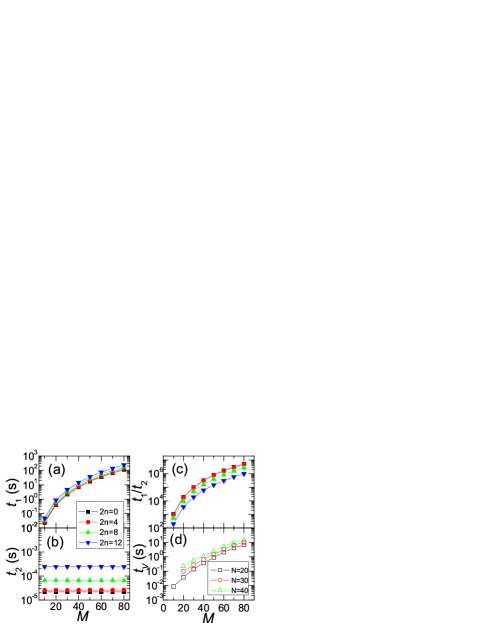
Figure 1: (color online) (a), CPU time, $t_{1}$, for the conventional method, as a function of $M$ and $2n$; (b), CPU time, $t_{2}$, for Eq.(3), as a function of $M$ and $2n$, (c), Ratio of $t_{1}$ to $t_{2}$; (d) Total CPU time, $t_{V}$, for $V_{0}$, $\mathbb{V}^{(1)}$ and $\mathbb{V}^{(2)}$, $N$ is the dimension of $\mathbb{V}^{(1)}$ and $\mathbb{V}^{(2)}$ with $1\leq i,j,k,l\leq N$.

The efficiency of the most important Eq. (3) is studied and the results are shown in Fig.1. Assuming $V_{0}$, $\mathbb{V}^{(1)}$ and $\mathbb{V}^{(2)}$ are available, the computational cost of Eq.(3) is $O((2n)^{4})$, which is independent of $M$. This implies Eq.(3) can be very conveniently extended to large model spaces. In contrast, the conventional method requires a time $O(M^{4}(2n)^{3})$ which highly depends on the model space due to the four-fold summation in Eq.(2). Testing calculations have been carried out on a Intel CPU with 2.4GHz. The elapsed time (in second), $t_{1}$ for the conventional method and $t_{2}$ for Eq. (3), are shown in Fig.1(a) and (b), respectively. To obtain the reliable $t_{1}(t_{2})$ value, identical calculations are repeated for many times (denoted by $m$, ranging from 10 to $10^{6}$) until the total elapsed time, $T$, is long enough, then $t_{1}(t_{2})=T/m$. From Fig.1(c), the ratio $t_{1}/t_{2}$ can be easily above the order of $10^{6}$ for $M=80$. Here, we chose $2n$ up to 12 because in the practical calculations, it seems enough to include up to 6-quasiparticle states.

However, the elapsed time, $t_{V}$, for $V_{0}$, $\mathbb{V}^{(1)}$ and $\mathbb{V}^{(2)}$ strongly depends on $M$. Moreover, $t_{V}$ is not included in $t_{2}$ and should be separately considered. Fortunately, all the $I_{2}$ matrix elements on top of the same ($\langle\Phi^{a}|$, $|\Phi^{b}\rangle$) pair share the common $V_{0}$, $\mathbb{V}^{(1)}$ and $\mathbb{V}^{(2)}$. Thus they are evaluated just one time for given HFB vacua, $|\Phi^{a}\rangle$ and $|\Phi^{b}\rangle$. Notice that the computational cost of $\mathbb{V}^{(1)}$ and $\mathbb{V}^{(2)}$ also depends on their dimension, $N$, with $1\leq i,j,k,l\leq N$. To cover all the $I_{2}$ matrix elements, $N$ should be properly chosen in the range of $2n\leq N\leq 2M$. Most of $t_{V}$ is taken by $\mathbb{V}^{(2)}$, whose computational cost is $O(M^{4}N)$. The $t_{V}$ values for various $M,N$ are shown in Fig.1(d). Comparing with $t_{1}$, it looks that $t_{V}\approx 0.1t_{1}$ at large $M$. Let us denote by $M_{I}$ the dimension of the $I_{2}$ matrix, and the global efficiency of Eq.(3) relative to the conventional method can be evaluated through $r=\frac{M_{I}^{2}t_{1}}{t_{V}+M_{I}^{2}t_{2}}$. Suppose $M_{I}=100,M=80$, $r$ can be easily in the order of $10^{5}$.

In Fig.1(d), the CPU time, $t_{V}$ is within several seconds for $M\leq 80$, calculations may be implemented when one directly uses Eq.(2), as is also taken in the standard $M-$scheme shell model methods. However, $t_{V}$ can drastically increase with $M$ bigger and bigger. Therefore, for heavy nuclei, one has to seek a more concise form of two-body interaction, such as separable interactions [31, 32], instead of directly using Eq.(2). For instance, the Projected Shell Model (PSM) uses the quadruple plus pairing interaction. The present method may be conveniently applied to develop the PSM, so that it may includes the states with more quasiparticles(e.g., 6-q.p., 8-q.p., etc).

5 Summary

In this letter, we focused on the matrix elements of one-body and two-body physical operators between arbitrary HFB states. The formula of Eq.(4), used by Bertsch and Robledo [16], has been extended to evaluate the matrix element of a product of single-fermion operators between two arbitrary HFB vacua [see Eq.(5)]. Start from Eq.(5), the matrix elements of physical operators have been successfully transformed into compact forms. Formulae for the pf$(\mathbb{S})=0$ case have also been given. Besides, the case of the Egido pole with $\langle\Phi^{a}|\Phi^{b}\rangle=0$ has been discussed. Testing calculations for the two-body operator matrix elements show that the new formulae can easily be in several orders faster than the conventional method. Thus those hopeless beyond mean field calculations for heavy nuclei in a large Fock space may be implemented by using the present method.

Acknowledgements Z.G. thanks Prof. Y. Sun and Dr. F.Q. Chen for the fruitful discussions and the manuscript. The work is supported by the National Natural Science Foundation of China under Contract Nos. 11175258, 11021504 and 11275068.

Appendix A Supplemental material

Supplementary material for mathematical details and the testing code can be found online at http://dx.doi.org/10.1016/j.physletb.2014.05.045.

References

[1] K. W. Schmid, Prog. Part. Nucl. Phys. 52 (2004) 565.
[2] G. E. Scuseria, C. A. Jiménez-Hoyos, T. M. Henderson, K. Samanta1 and J. K. Ellis, J. Chem. Phys. 135 (2011) 124108.
[3] N. Onishi and S. Yoshida, Nucl. Phys. 80 (1966) 367.
[4] P. Ring and P. Schuck, The Nuclear Many-Body Problem, Springer-Verlag, 1980.
[5] K. Hara and S. Iwasaki, Nucl. Phys. A 332 (1979) 61.
[6] K. Hara, A. Hayashi, and P. Ring, Nucl. Phys. A 385, (1982) 14.
[7] K. Neergård and E. Wüst, Nucl. Phys. A 402, (1983) 311.
[8] Q. Haider and D. Gogny, J. Phys. G 18 (1992) 993.
[9] F. Dönau, Phys. Rev. C 58 (1998) 872.
[10] M. Oi and N. Tajima, Phys. Lett. B 606 (2005) 43.
[11] M. Bender and P.-H. Heenen, Phys. Rev. C 78 (2008) 024309.
[12] L. M. Robledo, Phys. Rev. C 79 (2009) 021302(R).
[13] M. Oi and T. Mizusaki, Phys. Lett. B 707 (2012) 305.
[14] T. Mizusaki and M. Oi, Phys. Lett. B 715 (2012) 219.
[15] B. Avez and M. Bender, Phys. Rev. C 85 (2012) 034325.
[16] G. F. Bertsch and L. M. Robledo, Phys. Rev. Lett. 108 (2012) 042505.
[17] T. Mizusaki, M. Oi, Fang-Qi Chen, Yang Sun, Phys. Lett. B 725 (2013) 175.
[18] R. Balian and E. Brezin, Nuovo Cimento B 64 (1969) 37.
[19] S. Perez-Martin and L. M. Robledo, Phys. Rev. C 76 (2007) 064314.
[20] E. Lieb, J. Combinatorial Theory 5 (1968) 313.
[21] E.R. Caianiello, Combinatorics and Renormalization in Quantum Field Theory, Benjamin, 1973.
[22] Zao-Chun Gao, Qing-Li Hu, Y. S. Chen, Phys. Lett. B 732 (2014) 360.
[23] J.R. Stembridge, Advances in Mathematics, 83 (1990) 96.
[24] M. Ishikawa and M. Wakayama, J. Combinatorial Theory, A 88 (1999) 136.
[25] M. Ishikawa and M. Wakayama, Adv. Stud. Pure Math. 28 (2000) 133.
[26] M. Anguiano, J.L. Egido, L.M. Robledo, Nucl. Phys. A 696 (2001) 467.
[27]K. Hara and Y. Sun, Int. J. Mod. Phys. E 04 (1995)
637.
[28]C. Yannouleas and U. Landman, Rep. Prog. Phys. 70
(2007)2067.
[29]L. M. Robledo, Phys Rev C 50, (1994)2874.
[30]L. M. Robledo, Phys. Rev. C 84 (2011) 014307.
[31]Y. Tian, Z.-Y. Ma, and P. Ring, Phys Rev C 80 (2009)
024313.