Effective equations for matter-wave gap solitons in higher-order transversal states

Abstract

We demonstrate that an important class of nonlinear stationary solutions of the three-dimensional (3D) Gross-Pitaevskii equation (GPE) exhibiting nontrivial transversal configurations can be found and characterized in terms of an effective one-dimensional (1D) model. Using a variational approach we derive effective equations of lower dimensionality for BECs in $(m,n_{r})$ transversal states (states featuring a central vortex of charge $m$ as well as $n_{r}$ concentric zero-density rings at every $z$ plane) which provides us with a good approximate solution of the original 3D problem. Since the specifics of the transversal dynamics can be absorbed in the renormalization of a couple of parameters, the functional form of the equations obtained is universal. The model proposed finds its principal application in the study of the existence and classification of 3D gap solitons supported by 1D optical lattices, where in addition to providing a good estimate for the 3D wave functions it is able to make very good predictions for the $\mu(N)$ curves characterizing the different fundamental families. We have corroborated the validity of our model by comparing its predictions with those from the exact numerical solution of the full 3D GPE.

I I. INTRODUCTION

Matter-wave solitons are an important class of nonlinear excitations in Bose-Einstein condensates (BECs) Carre2 ; RevDS . They are coherent, spatially localized solutions of the Gross-Pitaevskii equation (GPE) resulting from a balance between linear dispersion and nonlinearity. Moreover, they are the atomic analogs of the optical solitons of nonlinear optics, with which they share many similarities KivGOP ; Kiv2D ; RMP-Malomed . This analogy has proved to be very fruitful and has stimulated much theoretical and experimental work in the field of Bose-Einstein condensation. A particular example of the interplay between the two fields which have attracted considerable attention in recent years is that of matter-wave gap solitons Kon1 ; Mor1 . These solitons, first observed experimentally in Ref. Ober1 , are localized nonlinear structures which can be realized in BECs loaded in one-dimensional (1D) optical lattices, and are characterized by a chemical potential lying in the forbidden band gaps of the underlying lineal problem.

Most theoretical treatments of matter-wave gap solitons in 1D optical lattices have been carried out in a 1D setting GS1D ; Kiv1 ; Abd1 ; Mal1 ; Wu1-2 . This approximation is justified when the condensate is subject to a transversal confinement so strong that its radial dynamics is frozen to the zero-point quantum fluctuations of the corresponding ground state. Under such circumstances, the axial dynamics can be accurately described in terms of the 1D GPE. However, as the transversal confinement decreases or the condensate density increases, the contribution from higher-order radial modes becomes more and more important so that transversal excitations can no longer be neglected VDB7 . This situation occurs frequently in practice.

In general, the study and characterization of matter-wave dark or gap solitons proceeds in different and well separated stages Carre1 . The first step consists in establishing the existence of such nonlinear solutions which, for solitons with a nontrivial radial configuration, requires solving the nonlinear eigenvalue problem associated with the three-dimensional (3D) GPE. This is a complex problem which is commonly addressed numerically by using a Newton continuation method in terms of the chemical potential of the condensate. In a subsequent step one usually is interested in the stability properties of the nonlinear states previously found. Such properties can be determined from a linear stability analysis based on the numerical solution of the Bogoliubov–de Gennes equations or by monitoring the long-time behavior of the condensate after a sudden small perturbation, which in turn requires the numerical integration of the equations of motion. In a final stage, one may be interested in the stabilization of certain unstable solutions, for instance, by changing the system configuration, the number of particles, or by introducing convenient pinning potentials or even a second component with repulsive interspecies interactions. In general, the different stages of the analysis have to be tackled separately by using different specific computational techniques. In what follows we will focus on the first stage. More specifically, we will be interested in the search for axially localized nonlinear stationary solutions of the 3D GPE exhibiting a higher-order radial configuration. While, in principle, this is a 3D problem where both axial and radial degrees of freedom can play an equally relevant role GS-3D , we will show in this work that, rather unexpectedly, it can be addressed in terms of an equivalent effective problem of lower dimensionality. Such dimensionality reduction is particularly interesting because the computational complexity of a Newton continuation method increases rapidly as one passes from 1D to 3D.

Effective equations of reduced dimensionality have proven to be a valuable tool in the description of BECs in highly anisotropic geometries. This class of systems, which can be realized by applying a strong confinement potential in one or two spatial directions, has received considerable attention in recent years Olsha1 ; Kett1 ; Das1 ; Strin1 ; VDB1 ; Guerin1 ; Isa1 . In particular, they are especially relevant for applications of trapped Bose condensates in matter-wave interferometry Shin2 ; Schumm1 ; Wang1 or in generation and manipulation of matter-wave dark Burger1 ; Brand1 and gap solitons Ober1 . Since highly anisotropic potentials induce two very different time scales in the condensate dynamics, in these systems the computational effort of a fully 3D treatment can become prohibitively high PRL06 ; Mott . This is so due to the fact that in order to guarantee the convergence of the numerical procedure one has to accurately resolve the fast degrees of freedom even though very often only the slow ones are relevant. Fortunately, the dynamics of dilute quantum gases tightly confined in the radial or the axial direction becomes effectively one dimensional or two dimensional, respectively, which allows for a description of the condensate dynamics in terms of effective equations of lower dimensionality. A number of such low-dimensional equations have been proposed Vic1 ; Jack1 ; Chio1 ; Gora ; Salas1 ; Kam1 ; Clark1 ; Yuka1 ; Ef1DEqs ; Nico1 . Especially relevant because of their simplicity and practical usefulness in realistic situations are those derived in Refs. Salas1 and Ef1DEqs . It has been shown that they can also be obtained from a variational approach based, respectively, on the appropriate energy and chemical-potential functionals Ef1DEqs . Several variants and extensions of the above two latter equations has also been proposed Modug1 ; Salas2 ; Salas3 ; Salas4 ; Adhik1 ; Adhik2 ; Adhik3 ; Carre3 ; Salas5 ; Adhik4 . For highly elongated condensates, it has been shown that, within their range of applicability, the effective equations derived in Refs. Salas1 and Ef1DEqs can accurately reproduce the experimental results Carre3 ; Kev1 ; Wel1 ; Kev2 . In fact, unlike what happens with the standard 1D GPE (which is a nonlinear Schrödinger equation with a cubic nonlinearity), the above mentioned effective equations can account properly for the contribution of transversal excitations on the axial dynamics of the condensate through a nonpolynomial nonlinear term. For this reason, they are particularly well suited for modeling trapped condensates in the dimensional crossover regime between 1D and 3D, a regime which is especially relevant in the study of matter-wave nonlinear structures such as dark and gap solitons.

Interestingly, the effective equations derived in this work are a natural generalization of the effective equations of Refs. Salas1 and Ef1DEqs to the case where the condensate exhibits a nontrivial higher-order transversal configuration. While stationary ringlike transversal excitations have been studied previously (both theoretically and experimentally) Kiv-RDS ; LCarr-RDS ; Kev-RDS1 ; San-RDS ; Kev-RDS2 ; Liu-RDS in BECs axially confined by a harmonic trapping potential (where the axial degrees of freedom play no relevant role), here we are mainly concerned with a quite different situation, where, in addition to a nontrivial radial configuration, the condensates feature a localized self-trapped nonlinear structure along the axial direction (such as occurs, for instance, in the case of matter-wave gap solitons in the weak-radial-confinement regime GS-3D ). In such circumstances, the axial degrees of freedom play as important role as the radial ones and thus must be explicitly incorporated in the physical description. As we will demonstrate, the effective equations derived in this work permit one to solve such an essentially 3D problem in terms of an equivalent 1D problem whose computational cost is similar to that corresponding to solving the standard 1D GPE.

II II. EFFECTIVE 1D MODEL

In the mean-field regime, the physics of dilute Bose-Einstein condensates at zero temperature, in a confining potential $V(\mathbf{r})$, is completely characterized by a macroscopic wave function $\psi(\mathbf{r},t)$ that satisfies the Gross-Pitaevskii equation GPE

$$i\hbar\frac{\partial\psi}{\partial t}=\left(-\frac{\hbar^{2}}{2M}\nabla^{2}+V(\mathbf{r})+gN\left|\psi\right|^{2}\right)\psi,$$ (1)

where $N$ is the number of atoms, and $g=4\pi\hbar^{2}a/M$ is the interaction strength determined by the s-wave scattering length $a$.

Equation (1) has been proven to accurately reproduce the dynamics of mean-field BECs under realistic experimental conditions PRL06 ; Mott . Our aim here is to look for a simpler effective equation of lower dimensionality which, under certain conditions, permit us to find good approximate solutions of the equation above. To this end, we start by assuming the adiabatic approximation to be applicable. More specifically, we shall assume that the axial degrees of freedom evolve so slowly in time in comparison with the transverse degrees of freedom that, at every instant $t$, the latter ones can relax almost instantaneously to a stationary state compatible with the axial configuration. Under these circumstances, correlations between axial and radial motions are negligible and the wave function can be factorized in the form Jack1

$$\psi(\mathbf{r},t)=\varphi(\mathbf{r}_{\bot};n_{1})\phi(z,t),$$ (2)

where $\mathbf{r}_{\bot}=(x,y)$ and $n_{1}$ is the axial linear density,

$$n_{1}(z,t)\equiv N\int d^{2}\mathbf{r}_{\bot}|\psi(\mathbf{r}_{\bot},z,t)|^{2}=N|\phi(z,t)|^{2}.$$ (3)

In the above equations, both $\psi$ and $\varphi$ have been normalized to unity.

Assuming, as is commonly the case, a separable confining potential $V(\mathbf{r})=V_{\bot}(\mathbf{r}_{\bot})+V_{z}(z)$, after substituting Eq. (2) into the GPE and averaging over the fast degrees of freedom one finally arrives at the following effective 1D equation governing the slow axial dynamics of the condensate Ef1DEqs :

$$i\hbar\frac{\partial\phi}{\partial t}=-\frac{\hbar^{2}}{2M}\frac{\partial^{2}\phi}{\partial z^{2}}+V_{z}(z)\phi+\mu_{\bot}(n_{1})\phi,$$ (4)

where $\mu_{\bot}(n_{1})$ is the local chemical potential satisfying the stationary transverse GPE

$$\left(-\frac{\hbar^{2}}{2M}\nabla_{\bot}^{2}+V_{\bot}(\mathbf{r}_{\bot})+gn_{1}\left|\varphi\right|^{2}\right)\varphi=\mu_{\bot}(n_{1})\varphi.$$ (5)

In what follows, we shall restrict ourselves to condensates confined in cylindrically symmetric traps which are harmonic in the radial direction,

$$V(\mathbf{r})=\frac{1}{2}M\omega_{\bot}^{2}r_{\bot}^{2}+V_{z}(z).$$ (6)

Under these circumstances, in the ideal-gas linear regime ($an_{1}\rightarrow 0$), the stationary transverse equation (5) can be exactly solved in terms of generalized Laguerre polynomials, $L_{n_{r}}^{(|m|)}(\rho^{2})$, and its solutions take the form

$$\varphi_{n_{r}}^{(m)}(\rho,\theta)=N_{n_{r}}^{(m)}e^{im\theta}\rho^{|m|}e^{-\rho^{2}/2}L_{n_{r}}^{(|m|)}(\rho^{2}),$$ (7)

where $N_{n_{r}}^{(m)}$ is the normalization constant,

$$N_{n_{r}}^{(m)}\equiv\sqrt{\frac{n_{r}!}{\pi a_{\bot}^{2}(n_{r}+|m|)!}}\;;$$ (8)

$\theta$ is the azimuthal angle; and $\rho\equiv r_{\bot}/a_{\bot}$ is the dimensionless radial coordinate, with $a_{\bot}=\sqrt{\hbar/M\omega_{\bot}}$ being the harmonic-oscillator length. In the equation above, $n_{r}=0,1,2,\ldots$ is the radial quantum number, and $m=0,\pm 1,\pm 2,\ldots$ is the axial angular momentum quantum number, which accounts for the presence of an axisymmetric vortex of charge $m$ (with $m=0$ corresponding to the absence of vortices). Using the following explicit expression for the generalized Laguerre polynomials Abramo :

$$L_{n_{r}}^{(m)}(x)=\sum_{k=0}^{n_{r}}(-1)^{k}\begin{pmatrix}n_{r}+m\\ n_{r}-k\end{pmatrix}\frac{x^{k}}{k!},$$ (9)

Eq. (7) can be rewritten in the form

$$\varphi_{n_{r}}^{(m)}(\rho,\theta)\!=\!N_{n_{r}}^{(m)}e^{im\theta}e^{-\rho^{2}/2}\sum_{k=0}^{n_{r}}\!\frac{(-1)^{k}}{k!}\!\begin{pmatrix}n_{r}+|m|\\ n_{r}-k\end{pmatrix}\!\rho^{2k+|m|}$$ (10)

These wave functions, which are stationary states of the underlying linear problem with energies

$$E=(2n_{r}+|m|+1)\hbar\omega_{\bot},$$ (11)

will be our starting point in the search for solutions of Eq. (5) in the nonlinear regime.

In principle, solving Eq. (5) is equivalent to finding the stationary points of the energy functional

$$\frac{E[\varphi]}{N}\equiv\!\!\int\!d^{2}\mathbf{r}_{\bot}\left(\!\frac{\hbar^{2}}{2M}\left|\nabla_{\bot}\varphi\right|^{2}+V_{\bot}\left|\varphi\right|^{2}+\frac{1}{2}gn_{1}\left|\varphi\right|^{4}\!\right)\!,$$ (12)

with $n_{1}=N/L$ being the condensate linear density. However, as was demonstrated in Ref. Ef1DEqs , for repulsive interatomic interactions ($a>0$), when the search for the stationary points of $E[\varphi]$ is restricted to a subspace of trial functions (as is usually the case) a variational approach based on the chemical-potential functional

$$\mu_{\bot}[\varphi]\!\equiv\!\!\int\!d^{2}\mathbf{r}_{\bot}\varphi^{\ast}\!\left(\!-\frac{\hbar^{2}}{2M}\nabla_{\bot}^{2}+V_{\bot}(\mathbf{r}_{\bot})+gn_{1}\left|\varphi\right|^{2}\!\right)\!\varphi,$$ (13)

can produce more simple and yet more accurate results than the usual variational approach based on the energy functional. For this reason, in what follows we will look for variational solutions of Eq. (5) in terms of both functionals.

It is natural to choose as trial functions those given in Eq. (10) with the substitution $a_{\bot}\rightarrow\Gamma a_{\bot}$, where $\Gamma$ is a variational parameter characterizing the condensate width. Solutions of this kind are analytic continuations of the linear eigenfunctions that bifurcate from the different linear energy levels as one enters the nonlinear regime. Thus, associated with every set of quantum numbers $(m,n_{r})$ there exists a one-parameter family of nonlinear stationary solutions that reduce to the stationary states of the underlying linear problem, Eq. (10), in the limit $an_{1}\rightarrow 0$. This enables us to categorize the solutions of Eq. (5) into families, and associate a given family with a pair $(m,n_{r})$. Note that the existence of such solutions implies the conservation in the nonlinear regime of the topology that the condensates exhibit in the ideal-gas linear regime. In fact, in passing from linear to nonlinear stationary states of a given family not only is the vortex charge $m$ conserved (which is a direct consequence of the underlying rotational symmetry), but so is the number ($n_{r}$) of concentric zero-density rings (radial nodes). And this occurs despite the fact that the nonlinear solutions are, in general, superpositions of many linear modes with different $n_{r}$ quantum numbers.

Table 1: Parameters $\alpha$, $\eta$, and $\gamma$ for the first few radial modes $(|m|,n_{r})$ as follow from Eqs. (15)–(18).

$(|m|,n_{r}):$	(0,0)	(1,0)	(2,0)	(0,1)	(1,1)	(2,1)	(0,2)	(1,2)	(2,2)
$\alpha:$	1	2	3	3	4	5	5	6	7
$\eta:$	1	1/2	3/8	1/2	5/16	1/4	11/32	15/64	199/1024
$\gamma:$	1	1/4	1/8	1/6	5/64	1/20	11/160	15/384	199/7168

Substituting the trial functions into the energy functional (12), after a rather cumbersome calculation, one obtains

$$\frac{E(n_{1};\Gamma)}{N}=\frac{\hbar\omega_{\bot}}{2\Gamma^{2}}\left(\alpha+\alpha\Gamma^{4}+2\eta an_{1}\right),$$ (14)

where the parameters $\alpha$ and $\eta$, which contain all the dependence on the quantum numbers $(|m|,n_{r})$, are given by

$$\alpha \equiv\sum\limits_{i,j=0}^{n_{r}}C_{i}C_{j}\,(1+i+j+|m|)!\;,$$ (15)

$$\eta \equiv\!\sum\limits_{i,j,k,l=0}^{n_{r}}\!C_{i}C_{j}C_{k}C_{l}\,2^{-(i+j+k+l+2|m|)}(i\!+\!j\!+\!k\!+\!l\!+\!2|m|)!\;,$$ (16)

with

$$C_{i}=\frac{(-1)^{i}\sqrt{n_{r}!(n_{r}+|m|)!}}{i!(n_{r}-i)!(i+|m|)!}.$$ (17)

At this point, it is most convenient to introduce a new parameter $\gamma$, defined as

$$\gamma\equiv\eta/\alpha,$$ (18)

and to rewrite Eq. (14) in terms of $\alpha$ and $\gamma$. Minimization of this latter equation with respect to the variational parameter then leads to the following $z$-dependent condensate width:

$$\Gamma=\left(1+2\gamma an_{1}\right)^{1/4}.$$ (19)

Substituting back in Eq. (14) and using that $\mu_{\bot}(n_{1})=\partial E/\partial N$, one finds the following transverse local chemical potential:

$$\mu_{\bot}(n_{1})=\hbar\omega_{\bot}\alpha\frac{1+3\gamma an_{1}}{\sqrt{1+2\gamma an_{1}}}.$$ (20)

After inserting the above expression into the axial equation (4), one finally arrives at

$$i\hbar\frac{\partial\phi}{\partial t}=-\frac{\hbar^{2}}{2M}\frac{\partial^{2}\phi}{\partial z^{2}}+V_{z}(z)\phi+\hbar\omega_{\bot}\alpha\frac{1+3\gamma aN\left|\phi\right|^{2}}{\sqrt{1+2\gamma aN\left|\phi\right|^{2}}}\phi.$$ (21)

This is an effective 1D equation that governs the axial dynamics of elongated BECs whose transversal state is a nonlinear mode belonging to the $(m,n_{r})$ family. Such transversal states, which exhibit an axisymmetric vortex of charge $m$ and $n_{r}$ concentric zero-density rings, at every instant $t$ and $z$ plane are indistinguishable from a (stationary) axially homogeneous condensate satisfying Eq. (5) with a linear density $n_{1}(z,t)=N|\phi(z,t)|^{2}$ and quantum numbers $(m,n_{r})$.

Equation (21) is generally applicable to condensates with both attractive ($a<0$) and repulsive ($a>0$) interatomic interactions. In the latter case, as already said, a somewhat simpler equation can be derived by using directly the chemical-potential functional instead of the usual energy functional. Indeed, after substituting the above trial functions into Eq. (13), one obtains

$$\mu_{\bot}(n_{1};\Gamma)=\frac{\hbar\omega_{\bot}}{2\Gamma^{2}}\alpha\left(1+\Gamma^{4}+4\gamma an_{1}\right),$$ (22)

where the parameters $\alpha$ and $\gamma$ are those defined previously in Eqs. (15)–(18). Minimizing $\mu_{\bot}$ with respect to the variational parameter $\Gamma$, one now finds the $z$-dependent condensate width

$$\Gamma=\left(1+4\gamma an_{1}\right)^{1/4},$$ (23)

and, after substituting back in Eq. (22), one obtains the following local chemical potential:

$$\mu_{\bot}(n_{1})=\hbar\omega_{\bot}\alpha\sqrt{1+4\gamma an_{1}}.$$ (24)

Inserting this expression into Eq. (4), we find

$$i\hbar\frac{\partial\phi}{\partial t}=-\frac{\hbar^{2}}{2M}\frac{\partial^{2}\phi}{\partial z^{2}}+V_{z}(z)\phi+\hbar\omega_{\bot}\alpha\sqrt{1+4\gamma aN\left|\phi\right|^{2}}\phi.$$ (25)

This equation, like Eq. (21), is an effective 1D equation governing the axial dynamics of elongated BECs with $a>0$ in a $(m,n_{r})$ transversal state. Equations (21) and (25), as well as their time-independent counterparts, are the central results of this work. It is interesting to note that these effective equations exhibit the same functional form irrespective of the $(m,n_{r})$ transversal state involved. In fact, the details of the transversal dynamics enter the above equations only through the numerical values of the parameters $\alpha$ and $\gamma$, which account for the dilution effect that the different transversal configurations induce in the radially averaged condensate density. The numerical values of $\alpha$ and $\gamma$ for the first few $(|m|,n_{r})$ pairs, obtained from Eqs. (15)–(18), are given in Table 1. Note, in particular, that the parameter $\alpha$ can be conveniently rewritten as

$$\alpha=(2n_{r}+|m|+1).$$ (26)

This formula is a direct consequence of the fact that the local chemical potential (24) must reduce to the (linear) energy (11) in the $an_{1}\rightarrow 0$ limit.

In the particular case $n_{r}=0$, which corresponds to condensates whose transversal state contains only an axisymmetric vortex of charge $m$, expressions (15) and (16) become

$$\alpha=(1+|m|),$$ (27)

$$\eta=(1+|m|)\gamma=\frac{(2|m|)!}{2^{2|m|}(|m|!)^{2}}\equiv\beta_{m}^{-1},$$ (28)

so that the equations of motion (21) and (25) reduce, respectively, to the effective equations first derived in Refs. Salas3 and Ef1DEqs . It is thus clear that the equations derived in this work are natural generalizations of the effective equations obtained previously and reduce to them in the proper limit.

Simple closed expressions for the parameter $\gamma$ can also be obtained in other particular cases. For instance, setting $n_{r}=1$ in Eq. (16) yields

$$\gamma=\eta/\alpha=\frac{(2+3|m|)}{4(1+|m|)(3+|m|)}\beta_{m}^{-1}\;;$$ (29)

while, for $n_{r}=2$, after a rather lengthy calculation, one finds

$$\gamma=\frac{44+(95+41|m|)|m|}{64(1+|m|)(2+|m|)(5+|m|)}\beta_{m}^{-1}.$$ (30)

The validity of the effective equations derived above relies on both the applicability of the adiabatic approximation and the robustness of the $(m,n_{r})$ transversal state involved. For general dynamical problems with $n_{r}>0$, such conditions may represent a rather severe limitation. There are, however, physical situations where one is primarily concerned with the existence and classification of stationary nonlinear excited states. This occurs, for instance, in the search for localized nonlinear structures such as matter-wave dark and gap solitons. While the study of this kind of system has commonly been performed in a 1D setting in which the radial state plays no relevant role, one may also be interested in nonlinear excited modes corresponding to higher-order transversal states. In principle, such analysis would require solving numerically the stationary 3D GPE, which is a computationally expensive task. Moreover, the numerical solution of the corresponding nonlinear eigenvalue problem—based, in most cases, on a continuation method—depends critically on the possibility of starting the iterative procedure with a sufficiently good initial estimation for both the axial and the radial parts of the wave function, which are not known a priori. As we shall see, the time-independent counterparts of the effective 1D equations (21) and (25) prove to be valuable tools that permit one to overcome the above difficulties. Since for a stationary problem the radial degrees of freedom can always follow adiabatically the (static) axial configuration, it is clear that, in such cases, the validity of the adiabatic approximation is guaranteed. In fact, the stationary versions of the above effective 1D equations have a broader range of applicability than initially expected, as demonstrated by the fact that they are even able to reproduce rather accurately the physical properties of disk-shaped gap solitons in higher-order transversal states.

III III. MATTER-WAVE SOLITONS IN HIGHER-ORDER TRANSVERSAL STATES

While small differences between results from the effective equations (21) and (25) do exist (see Ref. Ef1DEqs ), in practice, however, they are not very important, so that, from a quantitative point of view, the choice of which one to use is a matter of personal preference. For condensates with repulsive interatomic interactions ($a>0$) it may be advantageous to use Eq. (25) because it is somewhat simpler and, furthermore, permits one to obtain fully analytical expressions for a number of important stationary physical magnitudes Ef1DEqs . For $a<0$, however, one necessarily has to resort to Eq. (21) which has the additional advantage that it is also valid for $a>0$. In what follows we shall consider condensates with $a>0$ and shall restrict ourselves to Eq. (25). To demonstrate its utility in the search for matter-wave dark and gap solitons in a 3D regime, next we shall compare, for a number of representative examples, the predictions from this equation with those from the exact numerical solution of the full 3D GPE with no approximations. To this end, throughout this work we consider a zero-temperature ⁸⁷Rb condensate (s-wave scattering length $a=5.29$ nm) in a harmonic radial trap, subject to different axial potentials $V_{z}(z)$, and look for stationary solutions of Eq. (25) of the form

$$\phi(z,t)=\phi_{0}(z)\exp(-i\mu t/\hbar),$$ (31)

where $\mu$ is the condensate chemical potential and its corresponding density amplitude $\phi_{0}(z)$ satisfies the stationary equation

$$\left(\!\!-\frac{\hbar^{2}}{2M}\frac{\partial^{2}}{\partial z^{2}}\!+\!V_{z}(z)\!+\!\hbar\omega_{\bot}\alpha\sqrt{1+4\gamma aN\left|\phi_{0}\right|^{2}}\right)\!\phi_{0}\!=\!\mu\phi_{0}.$$ (32)

Starting from a convenient initial guess and using $\mu$ as a continuation parameter, excited solutions of a nonlinear differential equation such as this one can be found numerically by means of a Newton continuation method. As we shall see below, by solving the above effective 1D problem one can find good approximate solutions of the corresponding 3D problem. Indeed, not only does the solution of Eq. (32) accurately provide the chemical potential $\mu$ of the 3D condensate as a function of its particle content $N$ (a functional dependence that is of primary interest in the characterization and classification of matter-wave gap solitons into different families), but also gives, via Eqs. (2) and (31), an estimate for the corresponding 3D wave function:

$$\psi_{n_{r}}^{(m)}(\mathbf{r},t)=\varphi_{n_{r}}^{(m)}(\mathbf{r}_{\bot};n_{1})\phi_{0}(z)\exp(-i\mu t/\hbar),$$ (33)

where $\varphi_{n_{r}}^{(m)}$ is given by Eqs. (7) and (8) with the substitution $a_{\bot}\rightarrow\Gamma a_{\bot}$ and, as follows from Eqs. (3) and (23), the $z$-dependent dimensionless condensate width $\Gamma$ takes the form

$$\Gamma=\left(1+4\gamma aN\left|\phi_{0}(z)\right|^{2}\right)^{1/4}.$$ (34)

Stationary solutions of the full 3D GPE (1) have been obtained numerically in a similar manner. As already said, however, in this case it is essential to start from an initial guess which is sufficiently good in both the axial and the radial directions. In this regard, a good strategy is to use the above 1D estimate (for a relatively small value of $\mu$), Eq. (33), as the starting point for the 3D problem. We have implemented the numerical continuation method in terms of a Laguerre-Fourier spectral basis and have carefully checked the convergence and accuracy of our results by using different basis sets.

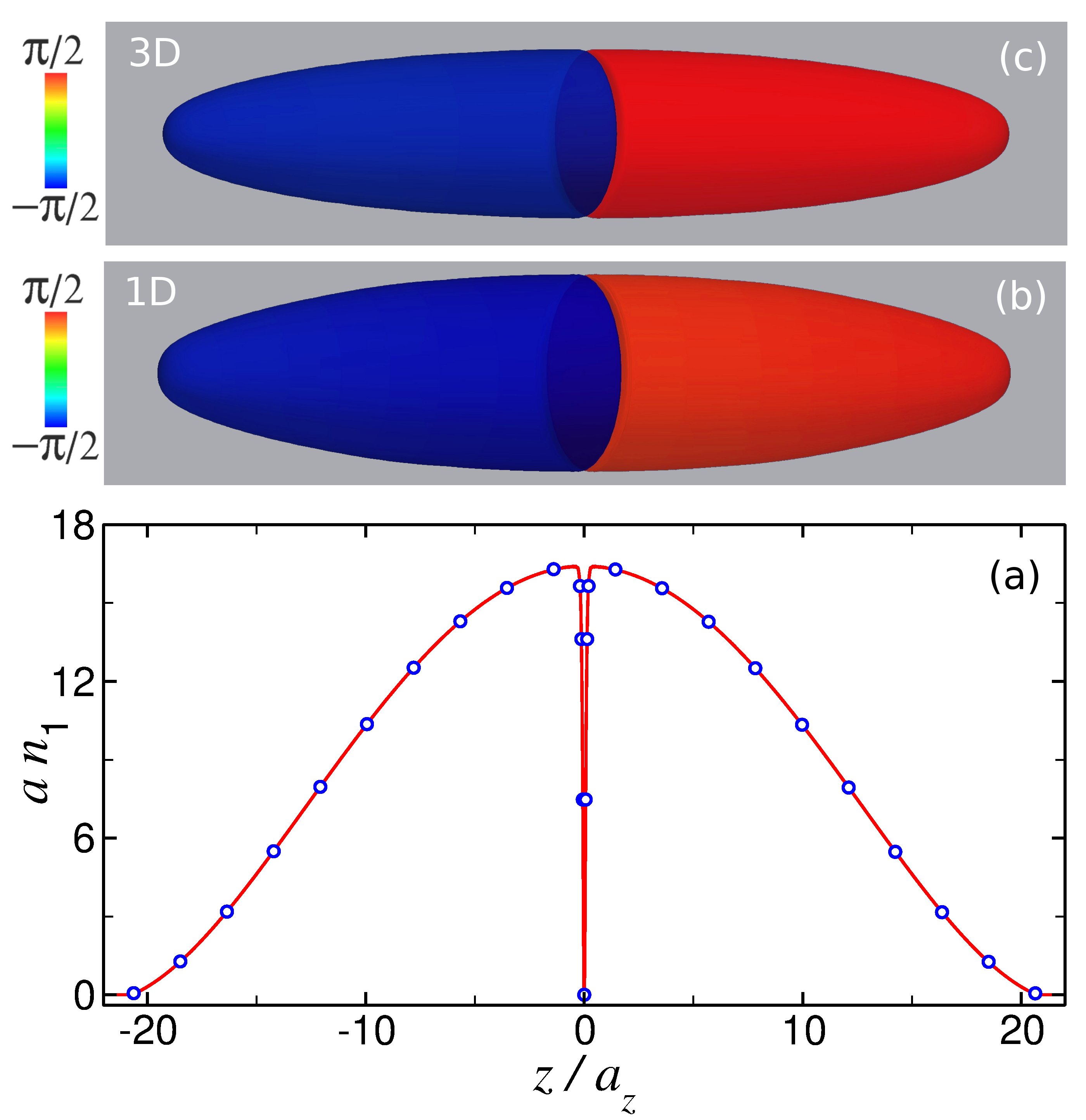
Figure 1: (Color online) 3D morphology of a stationary axial dark soliton in a $(0,0)$ transversal state generated in a ⁸⁷Rb condensate with $2\times 10^{5}$ atoms confined in a harmonic trap with frequencies $\omega_{z}=2\pi\times 15$ Hz and $\omega_{\bot}=2\pi\times 450$ Hz. (a) Dimensionless axial density $an_{1}$ as follows from the effective 1D equation (32) (solid red line) along with the corresponding 3D results (open circles) obtained from the full 3D GPE. The two upper panels show phase-colored density isosurfaces (taken at $5\%$ of the respective maxima) representing the 3D wave functions as obtained from (b) the effective 1D model and (c) the full 3D GPE. Panels (b) and (c) have been radially magnified by a factor of $5$. The color maps in these panels show that in both cases the condensate phase takes the constant value $-\pi/2$ to the left of the central density notch and $+\pi/2$ to the right. Lengths are given in terms of the axial oscillator length $a_{z}=$ $2.78$ $\mu$m.

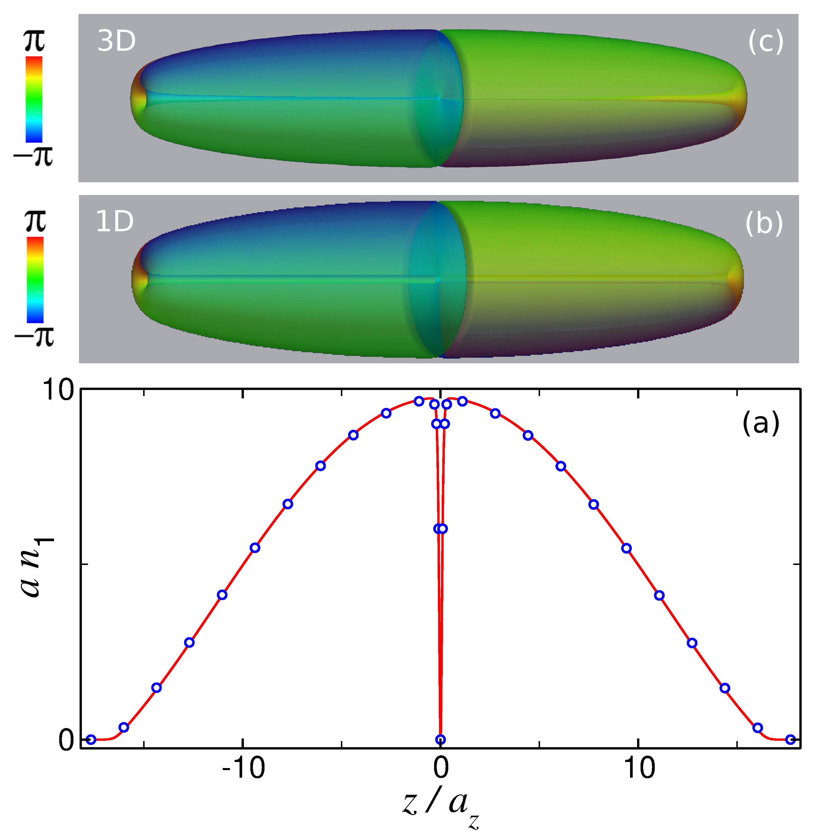
Figure 2: (Color online) Same as Fig. 1 but for a stationary axial dark soliton in a $(1,0)$ transversal state containing $10^{5}$ atoms. The color maps in panels (b) and (c) show that in both cases the condensate phase varies continuously from $-\pi$ to $+\pi$ around the vortex axis, while along the axial direction, for each azimuthal angle it exhibits a $\pi$-phase slip across the notch of zero density.

Figure 1 shows a stationary axial dark soliton in a $(0,0)$ transversal state generated in a ⁸⁷Rb condensate containing $2\times 10^{5}$ atoms confined in a harmonic trap with axial and radial frequencies $\omega_{z}=2\pi\times 15$ Hz and $\omega_{\bot}=2\pi\times 450$ Hz, respectively. Lengths in this figure are given in terms of the corresponding axial oscillator length $a_{z}=\sqrt{\hbar/M\omega_{z}}=$ $2.78$ $\mu$m. Figure 1(a) depicts the dimensionless axial density $an_{1}=aN|\phi_{0}(z)|^{2}$ as follows from the effective 1D equation (32) (solid red line) along with the corresponding 3D results (open circles) obtained from the full 3D GPE as prescribed by Eq. (3). Substituting the density amplitude $\phi_{0}(z)$ obtained from the solution of Eq. (32) into Eqs. (33) and (34), we have generated an effective 3D wave function which is shown in Fig. 1(b) as an isosurface of the atom density (taken at $5\%$ of its maximum) where the value of the phase of the wave function at each point is represented as a color map. Figure 1(c) displays the 3D wave function obtained from the numerical solution of the stationary version of the full 3D GPE (1) with no approximations. According to this latter equation, the condensate chemical potential takes the value $\mu=8.19\;\hbar\omega_{\bot}$, while the effective 1D equation (32) predicts $\mu=8.16\;\hbar\omega_{\bot}$ (which implies an error of only $0.35\%$). Even though in this case the transversal state is topologically trivial, it is nevertheless a linear superposition of many harmonic oscillator modes as reflects the fact that the chemical potential $\mu$ is much greater than the radial quantum $\hbar\omega_{\bot}$. In these circumstances, the standard 1D GPE is not applicable. In fact, this condensate clearly lies in the 3D regime, far away from the quasi-1D regime which would require $an_{1}\ll 1$, a condition that is not met as is evident from Fig. 1(a). Along the axial direction, however, both the density and the phase profiles exhibit the peculiar nontrivial structure of a dark soliton. Indeed, from Figs. 1(b) or 1(c) (which have been magnified along the radial direction by a factor of $5$ to facilitate the visualization) the characteristic $\pi$-phase slip across the notch of zero density is evident.

For the same confinement potential, Fig. 2 shows an axial dark soliton in a $(1,0)$ transversal state containing $10^{5}$ atoms. This corresponds to a stationary state of the GPE featuring a vortex of unit charge in the transversal direction in addition to a dark soliton in the axial direction. Figure 2(a) compares the prediction for the axial density $an_{1}$ (solid red line) obtained from Eq. (32) (which yields $\mu=6.56\;\hbar\omega_{\bot}$) with the exact numerical result (open circles) obtained from the 3D GPE (which yields $\mu=6.61\;\hbar\omega_{\bot}$). The phase-colored density isosurfaces shown in Figs. 2(b) and 2(c) represent, respectively, the corresponding 3D wave functions as obtained from the effective 1D model and the full 3D GPE. From these figures one can appreciate the complex phase structure of this nonlinear stationary state, which exhibits an azimuthal $2\pi$-phase slip in every $z$ plane besides a $\pi$-phase slip along the axial direction for each value of the azimuthal angle $\theta$.

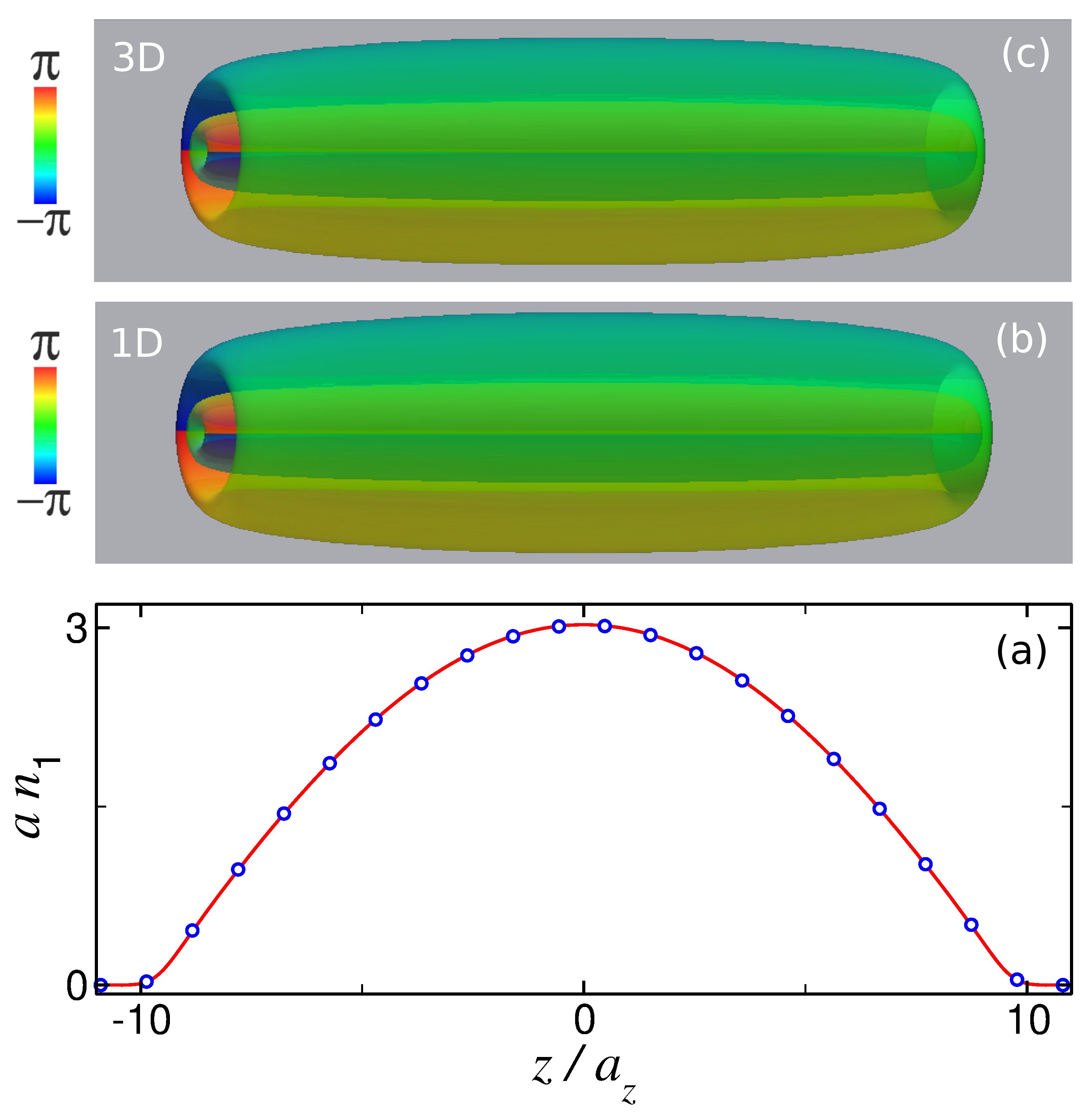
Figure 3: (Color online) Same as Fig. 1 but for a stationary state of the GPE with $2\times 10^{4}$ atoms in a $(1,1)$ transversal state with no axial nodes. In this case panels (b) and (c) have been radially magnified by a factor of $4$. The color maps in these panels show that in both cases the condensate phase varies continuously from $-\pi$ to $+\pi$ around the vortex axis while it exhibits a $\pi$ shift across the radial node for each azimuthal angle.

Figure 3 corresponds to a stationary state of the GPE with $2\times 10^{4}$ atoms in a $(1,1)$ transversal state with no axial nodes. In this case, at every $z$ plane the atom density features a central unit-charge vortex as well as a concentric zero-density ring, while the phase displays a $2\pi$ shift around the vortex singularity and a $\pi$ shift across the radial node (for each azimuthal angle) [see Figs. 3(b) and 3(c)]. As occurs with the previous cases, it is apparent that the effective 1D model (32) provides accurate predictions for both the axial density $an_{1}$ [Fig. 3(a)] and the chemical potential $\mu$ (in this case, it predicts $\mu=5.58\;\hbar\omega_{\bot}$ with an error less than $0.1\%$) and also gives a good estimate for the 3D wave function [Figs. 3(b) and 3(c)].

In what follows we shall assume the ⁸⁷Rb condensates to be loaded into a 1D optical lattice and look for gap solitons in higher-order transversal states. Specifically, we consider BECs confined in the radial direction by a harmonic potential of frequency $\omega_{\bot}=2\pi\times 240$ Hz and subject in the axial direction to a periodic potential of the form

$$V_{z}(z)=sE_{R}\sin^{2}\left(\pi z/d\right),$$ (35)

with $d=1.55$ $\mu$m being the lattice period and $s=15$ being the lattice depth in units of the recoil energy $E_{R}\equiv\hbar^{2}\pi^{2}/2Md^{2}$ [which, in turn, sets the typical energy scale of the underlying (noninteracting) linear problem]. These parameters correspond to a weak-radial-confinement regime characterized by a recoil energy $E_{R}$ of the same order as the quantum $\hbar\omega_{\bot}$ ($E_{R}/\hbar\omega_{\bot}=1$). In such a regime, the energy of gap solitons is always sufficiently large to excite higher modes of the radial confinement potential and thus 3D contributions are always relevant. 3D matter-wave gap solitons supported by 3D optical lattices have been studied in Ref. Kiv3D . Here, however, we are interested in 3D gap solitons supported by 1D lattices, a topic that has remained largely unexplored GS-3D . While matter-wave gap solitons in 1D lattices have received considerable attention, most studies have focused on an essentially 1D regime Kiv3 . However, the 3D weak-radial-confinement regime is of particular interest for a number of reasons GS-3D : (i) Gap solitons in this regime exhibit a rich radial structure reminiscent of that of the underlying linear problem. (ii) As a consequence of rotational symmetry, they can exist even inside the linear energy bands (embedded solitons Yang1 ). (iii) As occurs in the quasi-1D regime Wu1-2 , associated with each 3D linear spectral band there exists a family of fundamental gap solitons (stationary states highly localized in a single lattice site) that share common radial topological properties with the Bloch waves of the corresponding linear band; and finally, (iv) contrary to what would be commonly expected, the weak-radial-confinement regime supports long-lived gap solitons.

As is well known, in the noninteracting limit ($N\rightarrow 0$), the stationary states of a BEC in the presence of a 1D lattice are (delocalized) Bloch waves with energies lying in the allowed bands of the lattice band-gap spectrum. Because of the separability of axial and radial contributions in the linear Hamiltonian, the 3D spectrum follows from the 1D band-gap spectrum of the corresponding axial problem by simply adding the different allowed energies $E_{m,n_{r}}$ of the radial harmonic oscillator, Eq. (11). As a result, the 3D band-gap spectrum exhibits a series of replicas of the different 1D energy bands, shifted up in energy by integer multiples of $\hbar\omega_{\bot}$, with the different shifted bands reflecting the contribution of the different excited radial modes GS-3D . Different energy bands are characterized by the quantum numbers $(n,m,n_{r})$ where $n=1,2,3,\ldots$ is the band index of the corresponding 1D axial problem and $(m,n_{r})$ characterizes the radial state. Based on this fact, we introduced in Ref. GS-3D a nomenclature for gap solitons in the weak-radial-confinement regime. Indeed, adiabatic continuation of the chemical potential (or equivalently, the number of atoms $N$) permits connecting the different states of a given family and thus defines a trajectory in the $\mu$-$N$ plane that approaches a certain linear energy band as $N\rightarrow 0$. This enables us to categorize fundamental gap solitons into families and associate a given family with a linear band $(n,m,n_{r})$. Since gap solitons of type $(n,m,n_{r})$ can only appear for chemical potentials higher than that of the corresponding spectral band, it is clear that there exists a threshold chemical potential for each family. As $N$ increases or decreases, gap solitons in a family increase or decrease in size sharing, however, common topological properties.

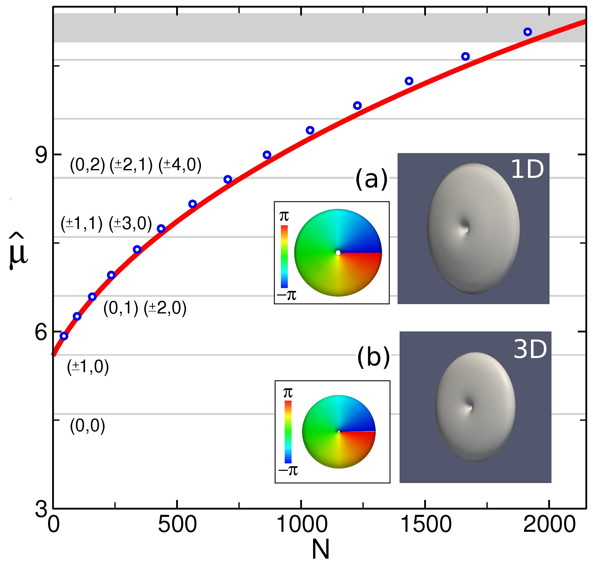
Figure 4: (Color online) Distinctive $\widehat{\mu}(N)$ curve characterizing the family of $(1,1,0)$ gap solitons, where $\widehat{\mu}$ stands for $\mu/\hbar\omega_{\bot}$. The solid red line is the result obtained from the effective 1D model (32), while open circles have been obtained from the numerical solution of the full 3D GPE. Horizontal gray strips represent the spectral bands of the underlying linear problem. The insets display an example of a soliton of this family with $N=500$ particles. The soliton wave function as obtained from the effective 1D model (32) is shown in panels (a) in terms of an isosurface of the atom density taken at $5\%$ of its maximum (right panel) and a color map of the local phase (left panel). Panels (b) show the corresponding results as obtained from the 3D GPE. The field of view in each panel is $6.1$ $\mu$m $\times$ $6.1$ $\mu$m. The color maps in panels (a) and (b) show that in both cases the condensate phase varies continuously from $-\pi$ to $+\pi$ around the vortex singularity.

Figure 4 shows the trajectory in the $\widehat{\mu}$-$N$ plane characterizing the family of $(1,1,0)$ gap solitons, where $\widehat{\mu}$ stands for the dimensionless chemical potential $\mu/\hbar\omega_{\bot}$. The solid red line is the result obtained from the effective 1D model (32) while open circles have been obtained from the numerical solution of the full 3D GPE. Both results agree to within $1.5\%$. In this and the following figures the horizontal gray strips represent the spectral bands of the underlying linear problem. The first seven (narrow) strips are different 3D replicas corresponding to the axial band index $n=1$ [only the quantum numbers $(m,n_{r})$ are represented in the figures]. The uppermost (wide) strip is the $(2,0,0)$ spectral band. In the insets we present an example of a soliton of this family with $N=500$ particles. The soliton wave function as obtained from the effective 1D model (32) is shown in panels (a) in terms of an isosurface of the atom density taken at $5\%$ of its maximum (right panel) and a color map of the local phase (left panel). Panels (b) show the corresponding results as obtained from the 3D GPE. The field of view in each panel is $6.1$ $\mu$m $\times$ $6.1$ $\mu$m. Gap solitons in this family are stationary disk-shaped condensates located at a single lattice site and featuring a central vortex of unit charge. While condensates with a similar look have been extensively studied in systems confined in the axial direction by a strong harmonic potential, it is important to note that gap solitons are completely different in nature. They are self-trapped nonlinear waves (bright solitons) resulting from an interplay between nonlinearity and periodicity which bifurcate from the linear Bloch bands and thus reside in the band gaps of the lattice spectrum. In particular, $(1,1,0)$ gap solitons are stationary states of the GPE featuring a vortex of unit charge in the transversal direction in addition to a (bright) gap soliton in the axial direction.

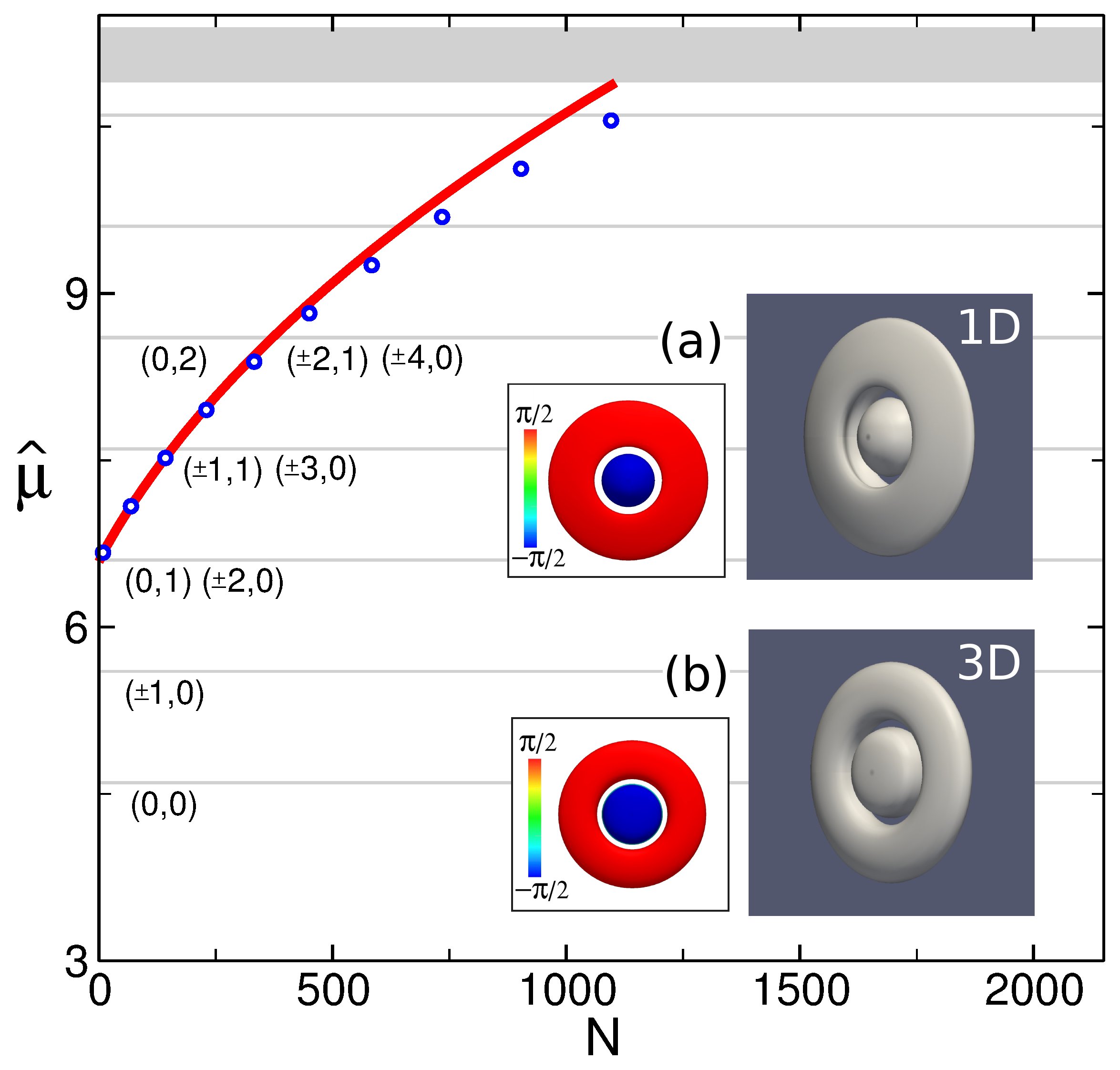
Figure 5: (Color online) Same as Fig. 4 but for the family of $(1,0,1)$ gap solitons. The color maps in panels (a) and (b) show that in both cases the condensate phase takes the constant value $-\pi/2$ inside the zero-density ring and $+\pi/2$ outside.

Figure 5 displays the distinctive $\widehat{\mu}(N)$ curve of the$\ (1,0,1)$ family. Even though in this case the prediction from the effective 1D model (32) (solid red line) is somewhat less accurate than before, it still agrees with the 3D results (open circles) to within $3\%$. As can be seen in the insets, the transversal profile of gap solitons in this family exhibit a concentric ring of zero density associated with a $\pi$-phase shift along the radial direction.

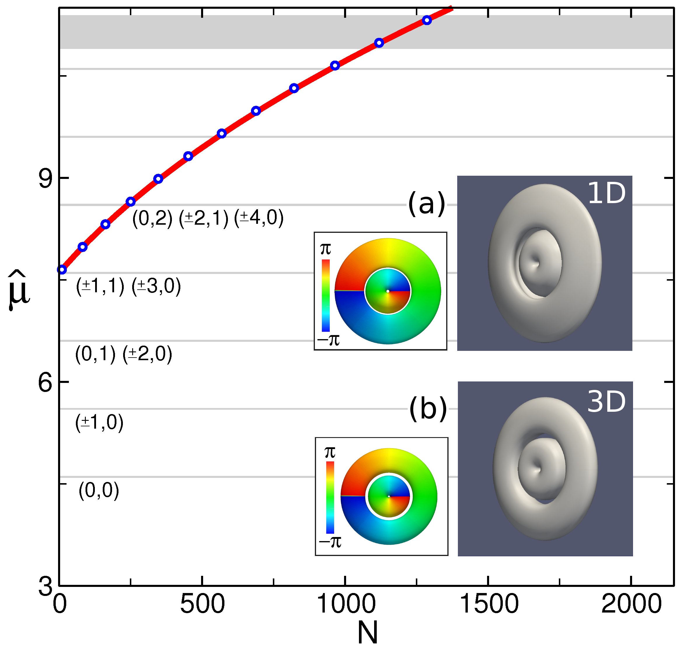
Figure 6: (Color online) Same as Fig. 4 but for the family of $(1,1,1)$ gap solitons. The color maps in panels (a) and (b) show that in both cases the condensate phase varies continuously from $-\pi$ to $+\pi$ around the vortex singularity, while it exhibits a $\pi$ shift across the concentric ring of zero density.

Finally, predictions for the $(1,1,1)$ and $(1,0,2)$ fundamental families are presented in Figs. 6 and 7, respectively. Gap solitons of type $(1,1,1)$ are self-trapped stationary states of the GPE featuring a central unit-charge vortex in addition to a concentric zero-density ring, while those of the $(1,0,2)$ family exhibit two concentric rings of zero density. As the figures reflect, the threshold chemical potentials for these families are greater than the previous ones. It is also apparent that the predicted $\widehat{\mu}(N)$ curves (solid red lines) are in excellent agreement with the exact numerical 3D results (open circles), being the error involved less than $1\%$ in both cases. Figures 4–7 also show that the effective 1D model (32) is able to provide a rather good estimate for the corresponding 3D wave functions.

IV IV. SUMMARY AND CONCLUSIONS

In this work we have demonstrated that an important class of nonlinear stationary solutions of the 3D GPE in the weak-radial-confinement regime can be found and characterized in terms of an effective 1D model. This model provides us with a good approximate solution of the original 3D problem involving, however, a technical complexity and computational effort similar to that corresponding to the standard 1D GPE.

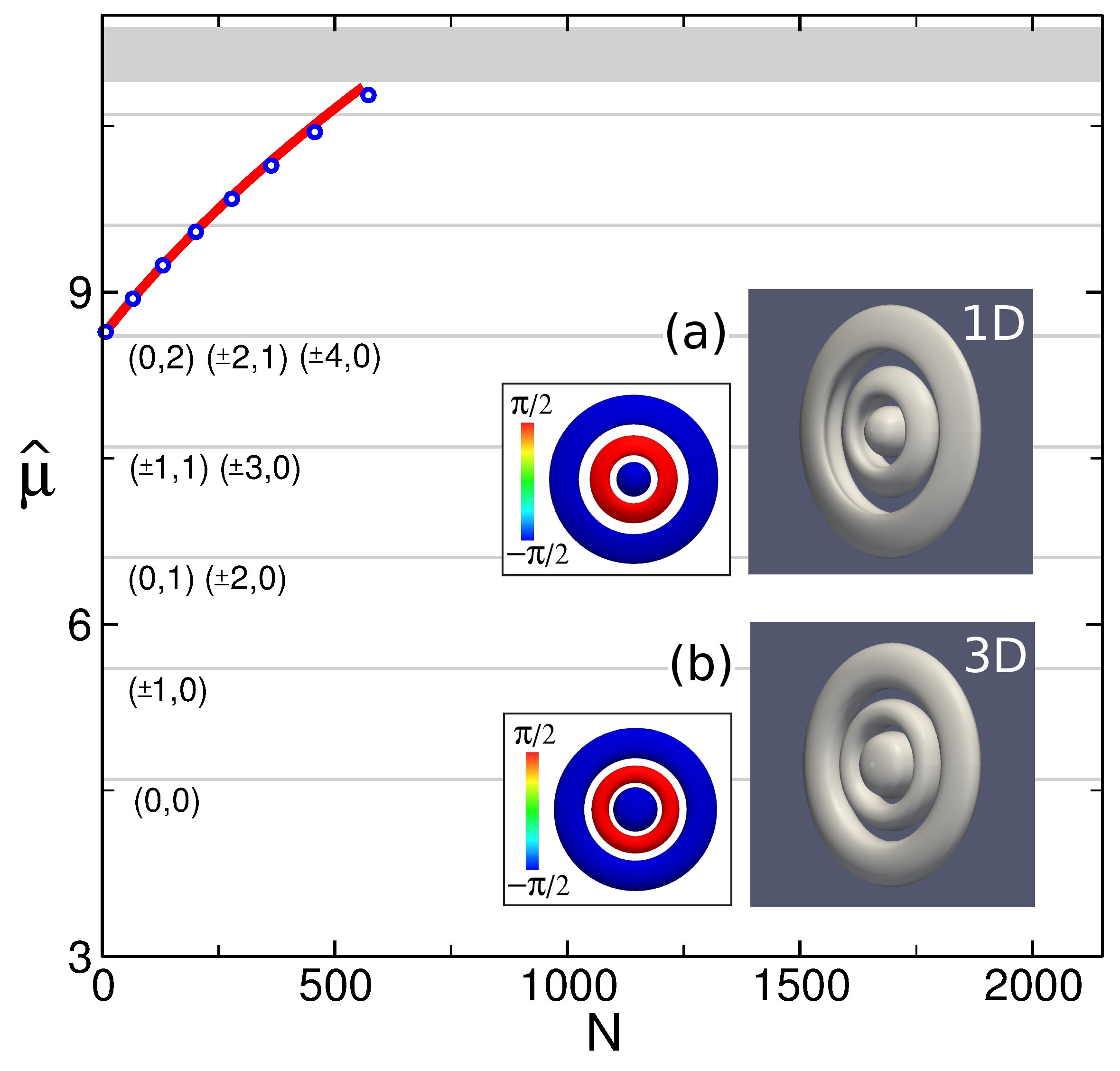
Figure 7: (Color online) Same as Fig. 4 but for the family of $(1,0,2)$ gap solitons. The color maps in panels (a) and (b) show that in both cases the condensate phase takes the constant value $-\pi/2$ in the innermost and outermost regions and $+\pi/2$ in between.

In the weak-radial-confinement regime the system energy is always large enough so that the 3D GPE admits stationary solutions exhibiting nontrivial higher-order transversal configurations. In order to address this problem in terms of an equivalent problem of lower dimensionality we have followed a variational approach based on both the energy and the chemical-potential functionals and have derived effective 1D equations that govern the axial dynamics of BECs in $(m,n_{r})$ transversal states, with $m$ and $n_{r}$ being, respectively, the axial angular momentum and the radial quantum numbers. Such states feature a central vortex of charge $m$ as well as $n_{r}$ concentric zero-density rings at every $z$ plane.

Interestingly, even though the equations derived in this work generalize previous proposals to the more complicated case of condensates exhibiting nontrivial 3D configurations, their functional forms are universal, which is a consequence of the fact that the specifics of the transversal dynamics can be absorbed in the renormalization of a couple of parameters ($\alpha$ and $\gamma$). This permits the study of systems of increasing complexity with the same computational effort.

The model proposed finds its principal application in those situations where one is primarily concerned with the existence and classification of axially localized nonlinear stationary states in a weak-radial-confinement regime. In these cases the numerical solution of the effective 1D problem provides an accurate prediction for the axial density profile and the chemical potential of the 3D condensate and gives a good estimate for the corresponding 3D wave function as well. In particular, the model proves to be a valuable tool in the study of the existence and classification of 3D gap solitons supported by 1D optical lattices, where it is able to make very good predictions for the important $\widehat{\mu}(N)$ curves, which are essential for characterizing the different fundamental families.

Matter-wave gap solitons in higher-order transversal states are of particular interest because they are a source for embedded gap solitons and, more importantly, they either are stable or are expected to be easily stabilized. In fact, it has been shown that $(1,0,0)$ gap solitons are stable even in the weak-radial-confinement regime GS-3D . The same occurs with the family $(1,1,0)$ GS-3D . Gap solitons of type $(1,m,0)$ with $m>1$ can be stabilized by simply changing their particle content GS-3D . On the other hand, it has been shown that BECs with a transversal profile similar to that of the family $(1,0,1)$, confined in a pancake trap, can be stabilized by adding a second component Kev-RDS2 . Since the instability of the $(1,0,1)$ family is purely transversal in nature, the same is expected to occur in the case of gap solitons. This strategy could also be used to stabilize gap solitons of type $(1,m,n_{r})$. Alternatively, specifically engineered pinning potentials might also be used to this purpose Bosh1 .

While a detailed stability analysis of these nonlinear structures is of great interest, it requires a separate study with specific computational techniques, distinct from those required for their generation and characterization. Such an analysis, which is beyond the scope of this work, will be the subject of a future publication.

References

- (1) Emergent Nonlinear Phenomena in Bose-Einstein Condensates: Theory and Experiment, edited by P. G. Kevrekidis, D. J. Frantzeskakis, and R. Carretero-González (Springer, Berlin, 2008).
- (2) D. J. Frantzeskakis, J. Phys. A: Math. Theor. 43, 213001 (2010).
- (3) Y. S. Kivshar and G. P. Agrawal, Optical Solitons: From Fibers to Photonic Crystals (Academic, San Diego, 2003).
- (4) E. A. Ostrovskaya and Y. S. Kivshar, Phys. Rev. Lett. 90, 160407 (2003).
- (5) Y. V. Kartashov, B. A. Malomed, and L. Torner, Rev. Mod. Phys. 83, 247 (2011).
- (6) V. A. Brazhnyi and V. V. Konotop, Mod. Phys. Lett. B 18, 627 (2004).
- (7) O. Morsch and M. Oberthaler, Rev. Mod. Phys. 78, 179 (2006).
- (8) B. Eiermann, Th. Anker, M. Albiez, M. Taglieber, P. Treutlein, K.-P.Marzlin, and M. K. Oberthaler, Phys. Rev. Lett. 92, 230401 (2004).
- (9) F. Kh. Abdullaev, B. B. Baizakov, S. A. Darmanyan, V. V. Konotop and M. Salerno, Phys. Rev. A 64, 043606 (2001).
- (10) P. J. Y. Louis, E. A. Ostrovskaya, C. M. Savage, and Y. S. Kivshar, Phys. Rev. A 67, 013602 (2003).
- (11) F. Kh. Abdullaev and M. Salerno, Phys. Rev. A 72, 033617 (2005).
- (12) T. Mayteevarunyoo and B. A. Malomed, Phys. Rev. A 74, 033616 (2006).
- (13) Y. Zhang and B. Wu, Phys. Rev. Lett. 102, 093905 (2009); Y. Zhang, Z. Liang, and B. Wu, Phys. Rev. A 80, 063815 (2009).
- (14) A. Muñoz Mateo, V. Delgado, and B. A. Malomed, Phys. Rev. A 83, 053610 (2011).
- (15) R. Carretero-González, D. J. Frantzeskakis, and P. G. Kevrekidis, Nonlinearity 21, R139 (2008).
- (16) A. Muñoz Mateo, V. Delgado, and B. A. Malomed, Phys. Rev. A 82, 053606 (2010).
- (17) M. Olshanii, Phys. Rev. Lett. 81, 938 (1998); D. S. Petrov, G. V. Shlyapnikov, and J. T. M. Walraven, ibid. 85, 3745 (2000); V. Dunjko, V. Lorent, and M. Olshanii, ibid. 86, 5413 (2001).
- (18) A. Görlitz, J. M. Vogels, A. E. Leanhardt, C. Raman, T. L. Gustavson, J. R. Abo-Shaeer, A. P. Chikkatur, S. Gupta, S. Inouye, T. Rosenband, and W. Ketterle, Phys. Rev. Lett. 87, 130402 (2001).
- (19) K. K. Das, Phys. Rev. A 66, 053612 (2002).
- (20) C. Menotti and S. Stringari, Phys. Rev. A 66, 043610 (2002); J. N. Fuchs, X. Leyronas, and R. Combescot, ibid. 68, 043610 (2003); F. Gerbier, Europhys. Lett. 66, 771 (2004).
- (21) A. Muñoz Mateo and V. Delgado, Phys. Rev. A 74, 065602 (2006).
- (22) W. Guerin, J.-F. Riou, J. P. Gaebler, V. Josse, P. Bouyer, and A. Aspect, Phys. Rev. Lett. 97, 200402 (2006).
- (23) J. Armijo, T. Jacqmin, K. Kheruntsyan, and I. Bouchoule, Phys. Rev. A 83, 021605(R) (2011); J. Armijo, Phys. Rev. Lett. 108, 225306 (2012).
- (24) Y. Shin, M. Saba, T. A. Pasquini, W. Ketterle, D. E. Pritchard, and A. E. Leanhardt, Phys. Rev. Lett. 92, 050405 (2004).
- (25) T. Schumm, S. Hofferberth, L. M. Andersson, S. Wildermuth, S. Groth, I. Bar-Joseph, J. Schmiedmayer and P. Krüger, Nat. Phys. 1, 57 (2005).
- (26) Y.-J. Wang, D. Z. Anderson, V. M. Bright, E. A. Cornell, Q. Diot, T. Kishimoto, M. Prentiss, R. A. Saravanan, S. R. Segal, and S. Wu, Phys. Rev. Lett. 94, 090405 (2005).
- (27) S. Burger, K. Bongs, S. Dettmer, W. Ertmer, K. Sengstock, A. Sanpera, G. V. Shlyapnikov, and M. Lewenstein, Phys. Rev. Lett. 83, 5198 (1999).
- (28) L. D. Carr, J. Brand, S. Burger, and A. Sanpera, Phys. Rev. A 63, 051601(R) (2001).
- (29) A. Muñoz Mateo and V. Delgado, Phys. Rev. Lett. 97, 180409 (2006).
- (30) J. A. M. Huhtamäki, M. Möttönen, T. Isoshima, V. Pietilä, and S. M. M. Virtanen, Phys. Rev. Lett. 97, 110406 (2006).
- (31) V. M. Pérez-García, H. Michinel, J. I. Cirac, M. Lewenstein, and P. Zoller, Phys. Rev. A 56, 1424 (1997).
- (32) A. D. Jackson, G. M. Kavoulakis, and C. J. Pethick, Phys. Rev. A 58, 2417 (1998).
- (33) M. L. Chiofalo and M. P. Tosi, Phys. Lett. A 268, 406 (2000).
- (34) A. E. Muryshev, G. V. Shlyapnikov, W. Ertmer, K. Sengstock, and M. Lewenstein, Phys. Rev. Lett. 89, 110401 (2002).
- (35) L. Salasnich, A. Parola, and L. Reatto, Phys. Rev. A 65, 043614 (2002); L. Salasnich, Laser Phys. 12, 198 (2002).
- (36) A. M. Kamchatnov and V. S. Shchesnovich, Phys. Rev. A 70, 023604 (2004).
- (37) M. Edwards, L. M. DeBeer, M. Demenikov, J. Galbreath, T. J. Mahaney, B. Nelsen, and C. W. Clark, J. Phys. B: At. Mol. Opt. Phys. 38, 363 (2005).
- (38) K.-P. Marzlin and V. I. Yukalov, Eur. Phys. J. D 33, 253 (2005).
- (39) A. Muñoz Mateo and V. Delgado, Phys. Rev. A 75, 063610 (2007); 77, 013617 (2008); Ann. Phys. 324, 709 (2009).
- (40) A. I. Nicolin and R. Carretero-González, Physica A 387, 6032 (2008); A. I. Nicolin and M. C. Raportaru, ibid. 389, 4663 (2010); A. I. Nicolin, ibid. 391, 1062 (2012); A. Balaž and A. I. Nicolin, Phys. Rev. A 85, 023613 (2012).
- (41) P. Massignan and M. Modugno, Phys. Rev. A 67, 023614 (2003); W. Zhang and L. You, ibid. 71, 025603 (2005).
- (42) L. Salasnich and B. A. Malomed, Phys. Rev. A 74, 053610 (2006); L. Salasnich, A. Cetoli, B. A. Malomed, F. Toigo, and L. Reatto, ibid. 76, 013623 (2007).
- (43) L. Salasnich, B. A. Malomed, and F. Toigo, and Phys. Rev. A 76, 063614 (2007).
- (44) L. Salasnich, J. Phys. A: Math. Theor. 42, 335205 (2009).
- (45) C. A. G. Buitrago and S. K. Adhikari, J. Phys. B: At. Mol. Opt. Phys. 42, 215306 (2009).
- (46) Luis E. Young-S., L. Salasnich, and S. K. Adhikari, Phys. Rev. A 82, 053601 (2010).
- (47) S. K. Adhikari, J. Phys. B: At. Mol. Opt. Phys. 44, 075301 (2011).
- (48) S. Middelkamp, J. J. Chang, C. Hamner, R. Carretero-González, P. G. Kevrekidis, V. Achilleos, D. J. Frantzeskakis, P. Schmelcher, and P. Engels, Phys. Lett. A 375, 642 (2011).
- (49) L. Salasnich and B. A. Malomed, J. Phys. B: At. Mol. Opt. Phys. 45, 055302, (2012).
- (50) P. Muruganandam, and S. K. Adhikari, Laser Phys. 22, 813, (2012).
- (51) S. Middelkamp, G. Theocharis, P. G. Kevrekidis, D. J. Frantzeskakis, and P. Schmelcher, Phys. Rev. A 81, 053618 (2010).
- (52) G. Theocharis, A. Weller, J. P. Ronzheimer, C. Gross, M. K. Oberthaler, P. G. Kevrekidis, and D. J. Frantzeskakis, Phys. Rev. A 81, 063604 (2010).
- (53) C. Wang, P. G. Kevrekidis, T. P. Horikis, D. J. Frantzeskakis, Phys. Lett. A, 374, 3863 (2010).
- (54) G. Theocharis, D. J. Frantzeskakis, P.G. Kevrekidis, B. A. Malomed, and Y. S. Kivshar, Phys. Rev. Lett. 90, 120403 (2003).
- (55) L. D. Carr and C. W. Clark, Phys. Rev. Lett. 97, 010403 (2006); Phys. Rev. A 74, 043613 (2006).
- (56) K. M. Mertes, J.W. Merrill, R. Carretero-González, D. J. Frantzeskakis, P. G. Kevrekidis, and D. S. Hall, Phys. Rev. Lett. 99, 190402 (2007).
- (57) M. Scherer, B. Lücke, G. Gebreyesus, O. Topic, F. Deuretzbacher, W. Ertmer, L. Santos, J. J. Arlt, and C. Klempt, Phys. Rev. Lett. 105, 135302 (2010).
- (58) J. Stockhofe, P. G. Kevrekidis, D. J. Frantzeskakis, P. Schmelcher, J. Phys. B: At. Mol. Opt. Phys. 44, 191003 (2011).
- (59) J. Li, D. S. Wang, Z. Y. Wu, Y. M. Yu, and W. M. Liu, Phys. Rev. A 86, 023628 (2012).
- (60) E. P. Gross, Nuovo Cimento 20, 454 (1961); J. Math. Phys. 4, 195 (1963); L. P. Pitaevskii, Zh. Eksp. Teor. Fiz. 40, 646 (1961) [Sov. Phys. JETP 13, 451 (1961)].
- (61) M. Abramowitz and I. Stegun, Handbook of Mathematical Functions (Dover, New York, 1972).
- (62) T. J. Alexander, E. A. Ostrovskaya, A. A. Sukhorukov, and Y. S. Kivshar, Phys. Rev. A 72, 043603 (2005).
- (63) M. Matuszewski, W. Królikowski, M. Trippenbach, and Y. S. Kivshar, Phys. Rev. A 73, 063621 (2006).
- (64) J. Yang, B. A. Malomed, and D. J. Kaup, Phys. Rev. Lett. 83, 1958 (1999); A. R. Champneys, B. A. Malomed, J. Yang, and D. J. Kaup, Physica D 152-153, 340 (2001); J. Yang, Phys. Rev. A 82, 053828 (2010).
- (65) K. Henderson, C. Ryu, C. MacCormick, and M. G. Boshier, New J. Phys. 11, 043030 (2009).