Drawing dynamical and parameter planes of iterative families and methods

Abstract

In this paper the complex dynamical analysis of the parametric fourth-order Kim’s iterative family is made on quadratic polynomials, showing the Matlab codes generated to draw the fractal images necessary to complete the study. The parameter spaces associated to the free critical points have been analyzed, showing the stable (and unstable) regions where the selection of the parameter will provide us excellent schemes (or dreadful ones).
Keywords: Nonlinear equation, Kim’s family, parameter space, dynamical plane, stability.

1 Introduction

It is usual to find nonlinear equations in the modelization of many scientific and engineering problems, and a broadly extended tool to solve them are the iterative methods. In the last decades, it has become an increasing and fruitful area of research. More recently, complex dynamics has revealed as a very useful tool to deep in the understanding of the rational functions that rise when an iterative scheme is applied to solve the nonlinear equation $f(z)=0$, with $f:\mathbb{C}\rightarrow\mathbb{C}$. The dynamical properties of this rational function give us important information about numerical features of the method as its stability and reliability.

There is an extensive literature on the study of iteration of rational mappings of complex variables (see [1, 2], for instance). The simplest and more deeply analyzed model is the obtained when $f(z)$ is a quadratic polynomial and the iterative process is Newton’s one. The dynamics of this iterative scheme has been widely studied (see, among others, [2, 5, 6]).

Just a decade ago that Varona in [3] and Amat et al. in [4] described the dynamical behavior of several well-known iterative methods. More recently, in [7, 8, 9, 10, 11, 12, 13, 16], the authors study the dynamics of different iterative families. In most of these studies, interesting dynamical planes, including some periodical behavior and other anomalies, have been obtained. In a few cases, the parameter planes have been also analyzed.

In order to study the dynamical behavior of an iterative method when is applied to a polynomial $p(z)$, it is necessary to recall some basic dynamical concepts. For a more extensive and comprehensive review of these concepts, see [5, 14].

Let $R:\mathbb{\hat{C}}\rightarrow\mathbb{\hat{C}}$ be a rational function, where $\mathbb{\hat{C}}$ is the Riemann sphere. The orbit of a point $z_{0}\in\mathbb{\hat{C}}$ is defined as the set of successive images of $z_{0}$ by the rational function, $\left\{z_{0},R(z_{0}),\ldots,R^{n}(z_{0}),\ldots\right\}$.

The dynamical behavior of the orbit of a point on the complex plane can be classified depending on its asymptotic behavior. In this way, a point $z_{0}\in\mathbb{C}$ is a fixed point of $R$ if $R(z_{0})=z_{0}$. A fixed point is attracting, repelling or neutral if $|R^{\prime}(z_{0})|$ is lower than, greater than or equal to 1, respectively. Moreover, if $|R^{\prime}(z_{0})|=0$, the fixed point is superattracting.

If $z^{*}_{f}$ is an attracting fixed point of the rational function $R$, its basin of attraction $\mathcal{A}(z^{*}_{f})$ is defined as the set of pre-images of any order such that

$$\mathcal{A}(z^{*}_{f})=\left\{z_{0}\in\mathbb{\hat{C}}:R^{n}(z_{0})\rightarrow z^{*}_{f},n\rightarrow\infty\right\}.$$

The set of points whose orbits tend to an attracting fixed point $z^{*}_{f}$ is defined as the Fatou set, $\mathcal{F}(R)$. The complementary set, the Julia set $\mathcal{J}(R)$, is the closure of the set consisting of its repelling fixed points, and establishes the borders between the basins of attraction.

In this paper, Section 2 is devoted to the complex analysis of a known fourth-order family, due to Kim (see [15]). The conjugacy classes of its associated fixed point operator, the stability of the strange fixed points, the analysis of the free critical points and the analysis of the parameter and dynamical planes are made. In Section 3, the Matlab code used to generate these tools is showed and the key instructions are explained in order to help to their eventual modification to adapt them to other iterative families. Finally, some conclusions are presented.

2 Complex dynamics features of Kim’s family

We will focus our attention on the dynamical analysis of a known parametric family of fourth-order methods for solving a nonlinear equation $f(x)=0$. Kim in [15] designs a class of optimal eighth-order methods, whose two first steps are

$$y_{k} = x_{k}-\frac{f(x_{k})}{f^{\prime}(x_{k})},$$

$$x_{k+1} = y_{k}-\frac{1+\eta u_{k}+\lambda u_{k}^{2}}{1+(\eta-2)u_{k}+\mu u_{k}^{2}}\frac{f(y_{k})}{f^{\prime}(x_{k})},$$ (1)

where $u_{k}=\frac{f(y_{k})}{f(x_{k})}$. We will suppose $\eta=\mu=0$. The result is a one-parametric family of iterative schemes whose order of convergence is four, with no conditions on $\lambda$.

In order to study the affine conjugacy classes of the iterative methods, the following Scaling Theorem can be easily checked.

Theorem 1

Let $g(z)$ be an analytic function, and let $A(z)=\alpha_{1}z+\alpha_{2}$, with $\alpha_{1}\neq 0$, be an affine map. Let $h(z)=\gamma(g\circ A)(z)$, with $\gamma\neq 0$. Let $O_{p}(z)$ be the fixed point operator of Kim’s family on the polynomial $p(z)$. Then, $(A\circ O_{h}\circ A^{-1})(z)=O_{g}(z)$, that is, $O_{g}(z)$ and $O_{h}(z)$ are affine conjugated by $A$.

This result allows up the knowledge of a family of polynomials with just the analysis of a few cases, from a suitable scaling.

In the following we will analyze the dynamical behavior of the fourth-order parametric family (2), on the quadratic polynomial $(z-a)(z-b)$, where $a,b\in\mathbb{C}$.

We apply the Möbius transformation

$$M(u)=\frac{u-a}{u-b},$$

whose inverse is

$$[M(u)]^{-1}=\frac{ub-a}{u-1},$$

in order to obtain the one-parametric operator

$$O_{p}(z,\lambda)=-\frac{z^{4}(1-\lambda+4z+6z^{2}+4z^{3}+z^{4})}{-1-4z-6z^{2}-4z^{3}+(-1+\lambda)z^{4}},$$ (2)

associated to the iterative method. In the study of the rational function (2), $z=0$ and $z=\infty$ appear as superattracting fixed points and $z=1$ is a strange fixed point for $\lambda\neq 1$ and $\lambda\neq 16$. There are also six strange fixed points more (a fixed point is called strange if it does not correspond to any root of the polynomial), whose analytical expression, depending on $\lambda$, is very complicated.

As we will see in the following, not only the number but also the stability of the fixed points depend on the parameter of the family. The expression of the differentiated operator, needed to analyze the stability of the fixed points and to define the critical points, is

$$O_{p}^{\prime}(z,\lambda)=-\frac{4z^{3}(1+z)^{4}(-(1+z)^{4}+\lambda(1-z+z^{2}-z^{3}+z^{4}))}{(1+4z+6z^{2}+4z^{3}-(-1+\lambda)z^{4})^{2}}.$$ (3)

As they come from the roots of the polynomial, it is clear that the origin and $\infty$ are always superattractive fixed points, but the stability of the other fixed points can change depending on the values of the parameter $\lambda$. In the following result we establish the stability of the strange fixed point $z=1$.

Theorem 2

The character of the strange fixed point $z=1$ is:

• If $\left|\lambda-16\right|>64$, then $z=1$ is an attractor and it cannot be a superattractor.

• When $\left|\lambda-16\right|=64$, $z=1$ is a parabolic point.

• If $\left|\lambda-16\right|<64$, being $\lambda\neq 1$ and $\lambda\neq 16$, then $z=1$ is a repulsor.

Proof.

It is easy to prove that

$$O_{p}^{\prime}\left(1,\lambda\right)=\frac{64}{16-\lambda}.$$

So,

$$\left|\frac{64}{16-\lambda}\right|\leq 1\phantom{aaa}\mbox{is equivalent to}\phantom{aaa}64\leq\left|16-\lambda\right|.$$

Let us consider $\lambda=a+ib$ an arbitrary complex number. Then,

$$64^{2}\leq 16^{2}-32a+a^{2}+b^{2}.$$

That is,

$$\left(a-16\right)^{2}+b^{2}\geq 64^{2}.$$

Therefore,

$$\left|O_{p}^{\prime}\left(1,\lambda\right)\right|\leq 1\ \ \mbox{if and only if}\ \ \left|\lambda-16\right|\geq 64.$$

Finally, if $\lambda$ verifies $\left|\lambda-16\right|<64$, then $\left|O_{p}^{\prime}\left(1,\lambda\right)\right|>1$ and $z=1$ is a repulsive point, except if $\lambda=1$ or $\lambda=16$, values for which $z=1$ is not a fixed point. ∎

The critical points of $O_{p}(z,\lambda)$ are $z=0$, $z=\infty$, $z=-1$ and

$$cr_{1}(\lambda) = \frac{1}{4}\left[1+\frac{1}{\lambda-1}-\beta-\sqrt{2}\sqrt{\frac{-5\lambda(6-7\lambda+\lambda^{2})}{(\lambda-1)^{3}}-\frac{(4+\lambda)\beta}{\lambda-1}}\right],$$

$$cr_{2}(\lambda) = \frac{1}{4}\left[1+\frac{1}{\lambda-1}-\beta+\sqrt{2}\sqrt{\frac{-5\lambda(6-7\lambda+\lambda^{2})}{(\lambda-1)^{3}}-\frac{(4+\lambda)\beta}{\lambda-1}}\right],$$

$$cr_{3}(\lambda) = \frac{1}{4}\left[1+\frac{1}{\lambda-1}+\beta-\sqrt{2}\sqrt{\frac{-5\lambda(6-7\lambda+\lambda^{2})}{(\lambda-1)^{3}}+\frac{(4+\lambda)\beta}{\lambda-1}}\right],$$

$$cr_{4}(\lambda) = \frac{1}{4}\left[1+\frac{1}{\lambda-1}-\beta+\sqrt{2}\sqrt{\frac{-5\lambda(6-7\lambda+\lambda^{2})}{(\lambda-1)^{3}}+\frac{(4+\lambda)\beta}{\lambda-1}}\right],$$

where $\lambda\neq 1$ and $\beta=\displaystyle\frac{\sqrt{5}\sqrt{(\lambda-1)^{2}}\sqrt{\lambda(4+\lambda)}}{(\lambda-1)^{2}}$.

The relevance of the knowledge of the free critical points (critical points different from the roots) is the following known fact: each invariant Fatou component is associated with, at least, one critical point.

Lemma 1

Analyzing the equation $O^{\prime}_{p}(z,\lambda)=0$, we obtain

• If $\lambda=0$, there is no free critical points of operator $O_{p}\left(z,0\right)$.

• If $\lambda=16$, then there are four free critical points: $z=-1$, $cr_{1}\left(16\right)=\frac{1}{4}\left(-\frac{4}{3}-\frac{8\sqrt{2}}{3}i\right)$, $cr_{2}\left(16\right)=\frac{1}{4}\left(-\frac{4}{3}+\frac{8\sqrt{2}}{3}i\right)$ and $cr_{3}\left(16\right)=cr_{4}\left(16\right)=1$.

• If $\lambda=-4$, then there are three different critical points: $z=-1$, $cr_{1}\left(-4\right)=cr_{3}\left(-4\right)=-i$ and $cr_{2}\left(-4\right)=cr_{4}\left(-4\right)=i$.

• In case of $\lambda=1$, the set of free critical points is $\{-1,-\frac{1}{2}+\frac{\sqrt{3}}{2}i,-\frac{1}{2}-\frac{\sqrt{3}}{2}i\}$.

• In any other case, $z=-1$, $cr_{1}\left(\lambda\right)$, $cr_{2}\left(\lambda\right)$, $cr_{3}\left(\lambda\right)$ and $cr_{4}\left(\lambda\right)$ are the free critical points.

Moreover, it can be proved that all free critical points are not independent, as $cr_{1}(\lambda)=\frac{1}{cr_{2}(\lambda)}$ and $cr_{3}(\lambda)=\frac{1}{cr_{4}(\lambda)}$.

Some of these properties determine the complexity of the operator, as we can see in the following results.

Theorem 3

The only member of the family whose operator is always conjugated to the rational map $z^{4}$ is the element corresponding to $\lambda=0$.

Proof.

From (2), we denote $p(z)=(1+z)^{4}(-(1+z)^{4}+\lambda(1-z+z^{2}-z^{3}+z^{4}))$ and $q(z)=(1+4z+6z^{2}+4z^{3}-(-1+\lambda)z^{4})^{2}$. By factorizing both polynomials, we can observe that the unique value of $\lambda$ verifying $p(z)=q(z)$ is $\lambda=0$. ∎

In fact, the element of Kim’s class corresponding to $\lambda=0$ is Ostrowski’s method. So, it is the most stable scheme of the family, as there are no free critical point and the iterations can only converge to any of the images of the roots of the polynomial. This is the same behavior observed when Ostrowski’s scheme was analyzed by the authors as a member of King’s family in [16].

Theorem 4

The element of the family corresponding to $\lambda=1$ is a fifth-order method whose operator is the rational map

$$O_{p}(z,\lambda)=\frac{z^{5}(2+z)(2+2z+z^{2})}{(1+2z)(1+2z+2z^{2})}.$$ (4)

Proof.

From directly substituting $\lambda=1$ in the rational operator (2), expression (4) is obtained, showing that $z=1$ is not a fixed point in this particular case. Moreover,

$$O_{p}^{\prime}(z,\lambda)=\frac{20z^{4}(1+z)^{4}\left(1+z+z^{2}\right)}{(1+2z)^{2}\left(1+2z+2z^{2}\right)^{2}},$$

and there exist only three free critical points. ∎

Then, in the particular case $\lambda=1$, the order of convergence is enhanced to five and, although there are three free critical points, they are in the basin of attraction of zero and infinity, as the strange fixed points are all repulsive in this case. So, it is a very stable element of the family with increased convergence in case of quadratic polynomials.

2.1 Using the parameter and dynamical planes

From the previous analysis, it is clear that the dynamical behavior of the rational operator associated to each value of the parameter can be very different. Different parameter spaces associated with free critical points of this family are obtained. The process to obtain these parameter planes is the following: we associate each point of the parameter plane with a complex value of $\lambda$, i.e., with an element of family (2). Every value of $\lambda$ belonging to the same connected component of the parameter space gives rise to subsets of schemes of family (2) with similar dynamical behavior. So, it is interesting to find regions of the parameter plane as much stable as possible, because these values of $\lambda$ will give us the best members of the family in terms of numerical stability.

As $cr_{1}(\lambda)=\frac{1}{cr_{2}(\lambda)}$ and $cr_{3}(\lambda)=\frac{1}{cr_{4}(\lambda)}$ (see Lemma 1), we have at most three independent free critical points. Nevertheless, $z=-1$ is pre-image of the fixed point $z=1$ and the parameter plane associated to this critical point is not significative. So, we can obtain two different parameter planes, with complementary information. When we consider the free critical point $cr_{1}(\lambda)$ (or $cr_{2}(\lambda)$) as a starting point of the iterative scheme of the family associated to each complex value of $\lambda$, we paint this point of the complex plane in red if the method converges to any of the roots (zero and infinity) and they are white in other cases. Then, the parameter plane $P_{1}$ is obtained; it is showed in Figure 1.

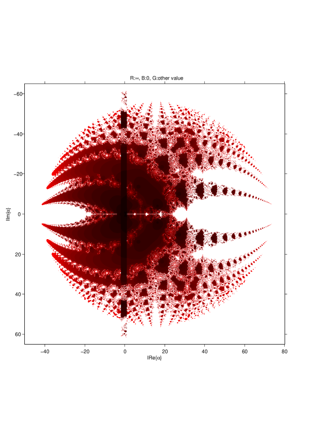
Figure 1: Parameter plane $P_{1}$ associated to $z=cr_{i}(\lambda)$, $i=1,2$

This figure has been generated for values of $\lambda$ in $[-50,80]\times[-65,65]$, with a mesh of $2000\times 2000$ points and 400 iterations per point. In $P_{1}$ the disk of repulsive behavior of $z=1$ is observed, showing different white regions where the convergence to $z\neq 0$, $z\neq\infty$ has been reached. An example of a dynamical plane associated to a value of the parameter is shown in Figure 2a, where three different basins of attraction appear, two of them of the superattractors $0$ and $\infty$ and the other of $z=1$, that is a fixed attractive point. It can be observed how the orbit (in yellow in the figure) converges asymptotically to the fixed point. Also in Figure 2b, the behavior in the boundary of the disk of stability of $z=1$ is presented, where this fixed point is parabolic. An orbit would tend to the parabolic point alternating two ”sides” (up and down the parabolic point, in this case).

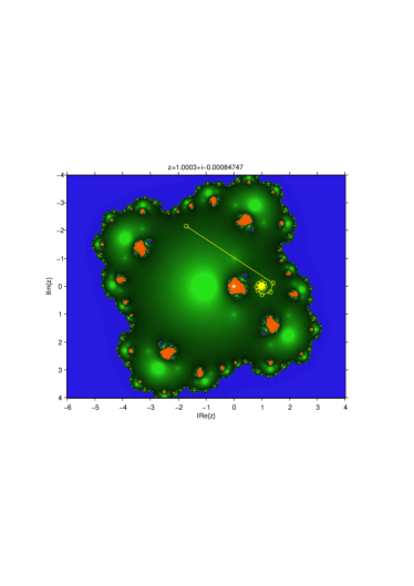
(a) $\left|\lambda-16\right|>64$

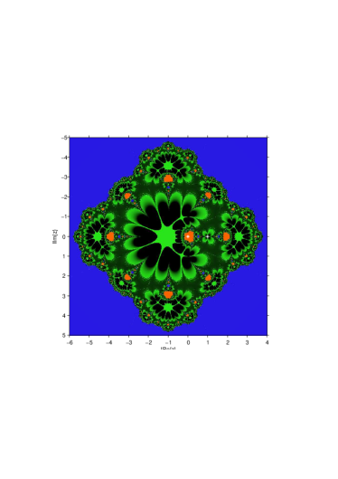
(b) $\left|\lambda-16\right|=64$

Figure 2: Dynamical planes for $\lambda$ verifying $\lambda$ verifying $\left|\lambda-16\right|\geq 64$

The generation of dynamical planes is very similar to the one of parameter spaces. In case of dynamical planes, the value of parameter $\lambda$ is constant (so, the dynamical plane is associated to a concrete element of the family of iterative methods). Each point of the complex plane is considered as a starting point of the iterative scheme and it is painted in different colors depending on the point which it has converged to. A detailed explanation of the generation of these graphics, joint with the Matlab codes used to generate them is provided in Section 3.

In Figure 3a, a detail of the region around $\lambda=0$ is seen. Let us notice that region around the origin is specially stable, specifically the vertical band between $-4$ and $1$ (see also Figure 2b).

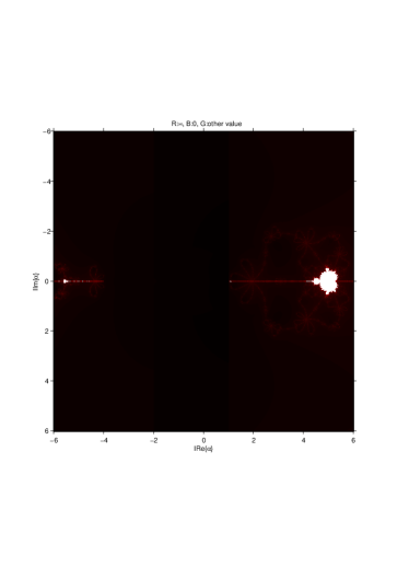
(a) Detail of $P_{1}$

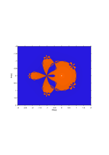
(b) Dynamical plane for $\lambda=1$

Figure 3: Around the origin

In fact, for $\lambda=0$, the associated dynamical plane is just a disk and its complementary in $\mathbb{C}$, as in Newton’s method. Around the origin is also very stable, with two connected components in the Fatou set. When $\lambda=16$, $z=1$ is not a fixed point (see Theorem 2) and $\{-1,1\}$ defines a periodic orbit of period 2 (see Figure 4). The singularity of this value of the parameter can be also observed in Figure LABEL:figure7(AÑADIR), in which a dynamical plane for $\lambda=15.9-0.2i$ is presented, showing a very stable behavior with only two basins of attraction, corresponding to the image of the roots of the polynomial by the Möbius map.

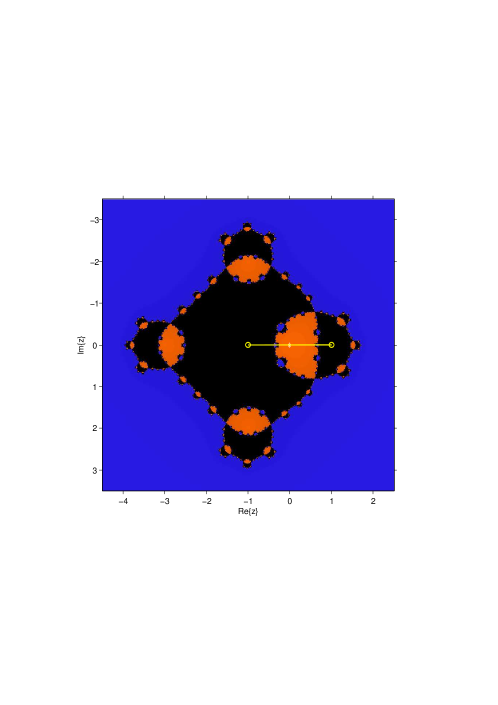
Figure 4: 2-periodic orbit for $\lambda=16$

It is also interesting to note in Figure 3a that white figures with a certain similarity with the known Mandelbrot set appear. Their antennas end in the values $\lambda=-4$ and $\lambda=1$, whose dynamical behavior is very different from the near values of the parameter, as was shown in Lemma 1.

A similar procedure can be carried out with the free critical points, $z=cr_{i}$, $i=3,4$, obtaining the parameter planes $P_{2}$, showed in Figure 5.

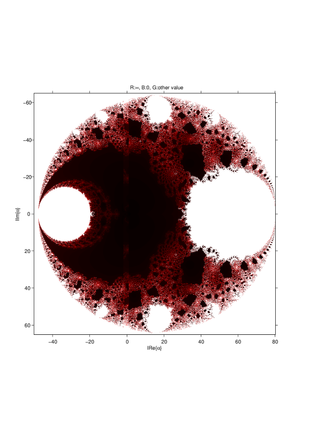
Figure 5: Parameter space $P_{2}$, associated to $z=cr_{i}$, $i=3,4$

As in case of $P_{1}$, the disk of repulsive behavior of $z=1$ is clear, and inside it different ”bulbs” appear, similar to disks. The biggest on the left of the real axis corresponds to the set of values of $\lambda$ where the fixed point $z=1$ has bifurcated in a periodic orbit of period two, as can be seen in Figure 6a. In the right of the real axis a bulb is the loci of two conjugated strange fixed points, see Figure 6b.

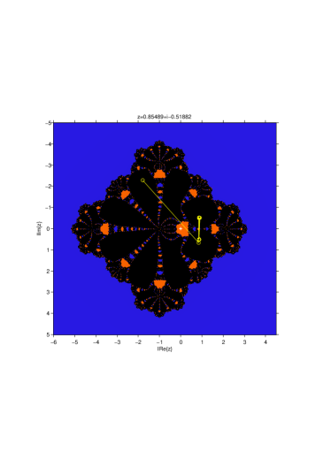
(a) 2-periodic orbit

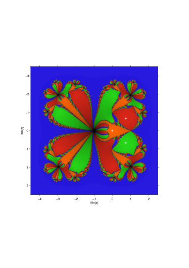
(b) Two atracting strange fixed points

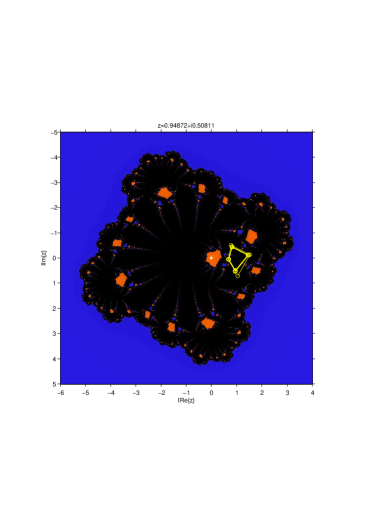
(c) 4-periodic orbit

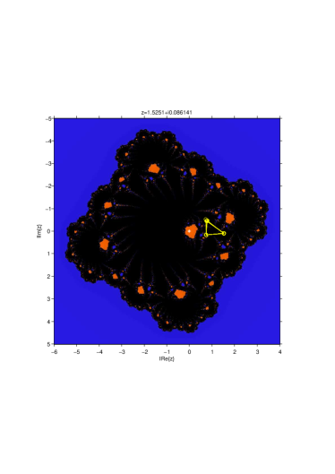
(d) 3-periodic orbit

Figure 6: Some dynamical planes from $P_{2}$

The bulbs on the top (see Figure 6c) and on the bottom of the imaginary axis correspond to periodic orbits of period 4. The rest of the bulbs surrounding the boundary of the stability disk of $z=1$ correspond to regions where periodic orbits of different periods appear. In fact, we can observe in Figure 6d) a periodic orbit of period 3, obtained from $\lambda=50+50i$ (comprobar). By applying Sharkovsky’s Theorem (see [14]), we can affirm that periodic orbits of arbitrary period can be found.

3 MATLAB^© planes code

The main goal of drawing the dynamical and parameters planes is the comprehension of the family or method behavior at a glance. The procedure to generate a dynamical or a parameter plane is very similar. However, there are significative differences, so both cases are developed below.

3.1 Dynamical planes

From a fixed point operator – that associates a polynomial to an iterative method – the dynamical plane illustrates the basins of attraction of the operator. The orbit of every point in the dynamical plane tends to a root (or to the infinity); this information, and the speed with which that the points tends to the root, can be displayed in the dynamical plane. In our pictures, each basin of attraction is drawn with a different color. Moreover, the brightness of the color points the number of iterations needed to reach the root of the polynomial.

The following code covers the Kim’s fixed point operators, when it is applied to a quadratic polynomial. This code has been utilized to generate the dynamical planes of several papers, as [9], [10] or [16]. (poner gato)

1  function  [I,it]=dynamicalPlane(lambda,bounds,points,maxiter)
2  
3   \%\% Description 
4   \% - dynamicalPlane obtains the dynamical plane of the Kim iterative method 
5    \% when it is applied to a quadratic polynomial. The dynamical plane is obtained 
6    \% as a ’points’-by-’points’-by-3 matrix ’I’, and can be displayed as 
7    \% >> imshow(I); 
8    \% moreover, the ’points’-by-’points matrix ’it’ records the number of 
9    \% iterations of each point. 
10    \% - the method is iterated till the ’maxiter’ iterations is reached, or 
11    \% till the estimation is enough close to the root. 
12    \% - it is mandatory the previous execution of 
13    \%   >> syms x 
14    \% bounds:   [min(Re(z)) max(Re(z)) min(Im(z)) max(Im(z))] 
15    \% test:     [I,it]=dynamicalPlane(0,[-1 1 -1 1],400,20); 
16      \% Values 
17  x0=bounds(1); xN=bounds(2); y0=bounds(3); yN=bounds(4); 
18  funfun=matlabFunction(fun);
19  
20  \% Fixed Point Operator 
21  syms x z
22  \% Kim’s operator 
23  Op=simple(-x.^4*(1-lambda+4*x+6*x^2+4*x^3+x^4)/(-1-4*x-6*x^2-4*x^3+x^4*(lambda-1))); 24      
25  \% Attracting points
26  fOp=matlabFunction(Op);
27  Opx=Op-x;
28  pf=double(solve(Opx));
29  dOp=diff(Op);
30  pc=double(solve(factor(dOp)));
31   adOp=matlabFunction(abs(dOp));
32   inda=double(abs(adOp(pf)))<=1;
33   pa=pf(inda==1);
34   if isempty(pa)
35     pa=double(solve(fun));
36   end
37   
38  \% Preparing the image
39      \% The image must have an odd number of points
40      if(mod(points,2)==0)
41          points=points+1;
42      end
43  
44      \% Complex mesh of points
45      dx=xN-x0; dy=yN-y0; d=max(dx,dy);
46      step=d/points;
47      x=x0:step:xN;
48      y=y0:step:yN;
49      [X,Y]=meshgrid(x,y);
50      z=complex(X,Y);
51  
52      \% Matrix startup
53      it=zeros(size(z));
54      r1=zeros(size(z)); r2=zeros(size(z)); r3=zeros(size(z));
55      R=zeros(size(z)); G=zeros(size(z)); B=zeros(size(z));
56  
57      \% Colour of each point
58      [f,col]=size(z);
59      for j=1:f
60          for k=1:col
61              s=z(j,k); rootfound=0;
62              while (rootfound==0 && it(j,k)<maxiter)
63                  s=fOp(s);
64                  it(j,k)=it(j,k)+1;
65                  if norm([real(s)-real(pa(1)) imag(s)-imag(pa(1))])<1e-3
66                      r1(j,k)=maxiter-1.5*it(j,k);
67                      R(j,k)=r1(j,k)/maxiter;
68                      G(j,k)=r1(j,k)/maxiter*102/255;
69                      rootfound=1;
70                elseiflength(pa)>1&&norm([real(s)-real(pa(2))imag(s)-imag(pa(2))])<1e-3
71                          r2(j,k)=maxiter-2*it(j,k);
72                          R(j,k)=r2(j,k)/maxiter*40/255;
73                          G(j,k)=r2(j,k)/maxiter*80/255;
74                          B(j,k)=r2(j,k)/maxiter;
75                          rootfound=1;
76                      elseif length(pa)>2&&norm([real(s)-real(pa(3)) imag(s)-imag(pa(3))])<1e-3
77                              r3(j,k)=maxiter-it(j,k);
78                              R(j,k)=r3(j,k)/maxiter*41/255;
79                              G(j,k)=r3(j,k)/maxiter*230/255;
80                              B(j,k)=r3(j,k)/maxiter*56/255;
81                              rootfound=1;
82                          end
83                      end
84                  end
85              end
86          end
87      end
88  
89  \% Image display
90  I(:,:,1)=R(:,:); I(:,:,2)=G(:,:); I(:,:,3)=B(:,:);
91  figure, imshow(I,’Xdata’,[x0 xN], ’Ydata’, [y0 yN])
92  axis on, axis xy, hold on
93  plot(real(pa),imag(pa),’w*’)
94  xlabel(’Re\{z\}’); ylabel(’Im\{z\}’);
95 axis xy

The code is divided into five different parts:

1. Values (lines 17–18).
   The bounds are renamed and the symbolic function introduced as fun is translated to an anonymous function, recallable by the output handle.

2. Fixed point operators (lines 23).
   

3. Calculation of attractive fixed points (lines 26–36).

4. Image creation (lines 39–94).
   Once the fixed point operator and the attracting points are set, the next step consists of the determination of the basins of attraction. The combination of the input parameters bounds and points set the resolution of the image, and it establishes the mesh of complex points (lines 39–50).

   Lines 58–87 are devoted to assign a color to each starting point. It depends on the basin of attraction and the number of iterations needed to reach the root. If the orbit tends to the attracting point set in the first index of line 35, the point is pictured in orange, as lines 67–69 show; for cases second and third, the point is pictured in blue (lines 72–74) and green (lines 78–80), respectively. Otherwise, the point is not modified, so its color is black.

   As the number of iterations needed to reach convergence increases, its corresponding color gets closer to white (black in the decreasing case). A coefficient in each case (lines 66, 71 and 77) is high if the number of iterations is low, and the RGB values are greater than in the slow orbit instance.

5. Image display (lines 90–94).
   The image display is based on the imshow command. Images are usually displayed in matrix form (from top to bottom and from left to right). In this case, the image is composed by complex points, so the natural display is the cartesian one (from bottom to top and from left to right). With this purpose, axis xy is written in line 95.

Once the program is executed, the output values are the image I and the number of iterations of each point it. Our recommendation is the use of the surf command to plot the number of iterations, in combination with the shading one.

In order to apply the introduced code to different fixed point operators, the only part to be changed is the fixed point operators corresponding one. If the method can converge to more than three points, just add another else if structure (as lines 79–84) and set a color as many times as necessary.

3.2 Parameter planes

  function  [a,I,c]=parametricplane(axini,axfin,ayini,ayfin,points,maxiter)
2  
3   \%\% Description 
4   \% - parametricplane obtains the parametric plane of the Kim iterative family 
5    \% when it is applied to a quadratic polynomial, associated with the free critical point cr_2.
6    \% [axini,axfin,ayini,ayfin] define the rectangle for possible values of the parameter \lambda 
7    \% points defines the mesh of size ’points’-by-’points’
8    \% maxiter is the maximum number of iterations of the method per value of \lambda 
9  
10    \% test:     [a,I,c]=parametricplane(-2,2,-2,2,500,25); 
11      \% Values 
12   
13  \% Preparing the image
14      \% The image must have an odd number of points
15      if(mod(points,2)==0)
16          points=points+1;
17      end
18  
19      \% Complex mesh of points
20   ax=linspace(axini,axfin,puntos);
21   ay=linspace(ayini,ayfin,puntos);
22   [AX,AY]=meshgrid(ax,ay);
23   a=complex(AX,AY);
24  
25      \% Matrices startup
26   I=zeros(puntos); c=zeros(puntos);
27 R=zeros(puntos); G=zeros(puntos); B=zeros(puntos);
57      \% Colour of each point
30      for j=1:points
31          for  k=1:points
32                 it=0;
33                  aa=a(j,k);
34                  c1=-((-4-aa)/(4*(-1+aa)))-(sqrt(5)*sqrt(4*aa+aa^2))/...
35                  (4*sqrt(1-2*aa+aa^2))+1/2*sqrt((-4-aa)^2/(2*(-1+aa)^2)...
36                  -(-6+aa)/(-1+aa)-(-2+2*aa)/(-1+aa)-((-((-4-aa)^3/(-1+aa)^3)...
37                  +(4*(-4-aa)*(-6+aa))/(-1+aa)^2-(8*(-4-aa))/(-1+aa))*sqrt(1-2*aa+aa^2))...
38                  /(2*sqrt(5)*sqrt(4*aa+aa^2)));
39                   while  it<maxiter  abs(c1)>1e-2 && it<maxiter && (abs(c1))<1000
40                      c1=-c1.^4*(-aa+(1+c1)^4)/(-1-4*c1-6*c1^2-4*c1^3+c1^4*(aa-1));
41                      it=it+1;
42                  end
43                  c(j,k)=c1;
44                  if  abs(c1)<1e-2
45                         R(j,k)=it/maxiter; 
46                  else if   abs(c1)>=1000 \|\|  ~isfinite(c1)
47                      R(j,k)=it/maxiter;
48                      else\color{black} 
49                      R(j,k)=1;
50                      G(j,k)=1;
51                      B(j,k)=1;
52                      end
53                  end
54              end
55          end
56  \% Image display
57  I(:,:,1)=R(:,:); I(:,:,2)=G(:,:); I(:,:,3)=B(:,:);
58  figure, imshow(I,’Xdata’,[x0 xN], ’Ydata’, [y0 yN])
59  axis on, axis xy, hold on
60  plot(real(pa),imag(pa),’w*’)
61  xlabel(’Re\{z\}’); ylabel(’Im\{z\}’);
62  axis xy

The code is divided into five different parts:

1. Values (lines 17–18).
   The bounds are renamed and the symbolic function introduced as fun is translated to an anonymous function, recallable by the output handle.

2. Fixed point operators (lines 23).
   

3. Calculation of attractive fixed points (lines 26–36).

4. Image creation (lines 39–94).
   Once the fixed point operator and the attracting points are set, the next step consists of the determination of the basins of attraction. The combination of the input parameters bounds and points set the resolution of the image, and it establishes the mesh of complex points (lines 39–50).

   Lines 58–87 are devoted to assign a color to each starting point. It depends on the basin of attraction and the number of iterations needed to reach the root. If the orbit tends to the attracting point set in the first index of line 35, the point is pictured in orange, as lines 67–69 show; for cases second and third, the point is pictured in blue (lines 72–74) and green (lines 78–80), respectively. Otherwise, the point is not modified, so its color is black.

   As the number of iterations needed to reach convergence increases, its corresponding color gets closer to white (black in the decreasing case). A coefficient in each case (lines 66, 71 and 77) is high if the number of iterations is low, and the RGB values are greater than in the slow orbit instance.

5. Image display (lines 90–94).
   The image display is based on the imshow command. Images are usually displayed in matrix form (from top to bottom and from left to right). In this case, the image is composed by complex points, so the natural display is the cartesian one (from bottom to top and from left to right). With this purpose, axis xy is written in line 95.

Once the program is executed, the output values are the image I and the number of iterations of each point it. Our recommendation is the use of the surf command to plot the number of iterations, in combination with the shading one.

In order to apply the introduced code to different fixed point operators, the only part to be changed is the fixed point operators corresponding one. If the method can converge to more than three points, just add another else if structure (as lines 79–84) and set a color as many times as necessary.

References

- [1] A. Douady, J.H. Hubbard, On the dynamics of polynomials-like mappings, Ann. Sci. Ec. Norm. Sup., 18 (1985) 287-343.
- [2] J. Curry, L. Garnet, D. Sullivan, On the iteration of a rational function: Computer experiments with Newton’s method, Comm. Math. Phys., 91 (1983) 267-277.
- [3] J.L. Varona, Graphic and numerical comparison between iterative methods, Math. Intelligencer, 24(1) (2002) 37-46.
- [4] S. Amat, S. Busquier, S. Plaza, Review of some iterative root-finding methods from a dynamical point of view, Scientia Series A: Mathematical Sciences, 10 (2004) 3-35.
- [5] P. Blanchard, The dynamics of Newton’s method, Proc. of Symposia in Applied Math., 49 (1994) 139-154.
- [6] N. Fagella, Invariants in dinàmica complexa, Butlletí de la Soc. Cat. de Matemàtiques, 23(1) (2008) 29-51.
- [7] J.M. Gutiérrez, M.A. Hernández and N. Romero, Dynamics of a new family of iterative processes for quadratic polynomials, J. of Computational and Applied Mathematics, 233 (2010) 2688-2695.
- [8] G. Honorato, S. Plaza, N. Romero, Dynamics of a high-order family of iterative methods, Journal of Complexity, 27 (2011) 221-229.
- [9] F. Chicharro, A. Cordero, J.M. Gutiérrez, J.R. Torregrosa, Complex dynamics of derivative-free methods for nonlinear equations, Applied Mathematics and Computation, doi: 10.1016/j.amc.2012.12.075.
- [10] S. Artidiello, F. Chicharro, A. Cordero, J.R. Torregrosa, Local convergence and dynamical analysis of a new family of optimal fourth-order iterative methods, International Journal of Computer Mathematics doi:10.1080/00207160.2012.748900.
- [11] M. Scott, B. Neta, C. Chun, Basin attractors for various methods, Applied Mathematics and Computation, 218 (2011) 2584-2599.
- [12] C. Chun, M.Y. Lee, B. Neta, J. Džunić, On optimal fourth-order iterative methods free from second derivative and their dynamics, Applied Mathematics and Computation, 218 (2012) 6427-6438.
- [13] B. Neta, M. Scott, C. Chun, Basin attractors for various methods for multiple roots, Applied Mathematics and Computation, 218 (2012) 5043-5066.
- [14] R.L. Devaney, The Mandelbrot Set, the Farey Tree and the Fibonacci sequence, Am. Math. Monthly, 106(4) (1999) 289-302.
- [15] Y. I. Kim, A triparametric family of three-step optimal eighth-order methods for solving nonlinear equations, International Journal of Computer Mathematics, 89(8) (2012) 1051-1059.
- [16] Alicia Cordero, Javier Garcia-Maimo, Juan R. Torregrosa, Maria P. Vassileva, Pura Vindel, Chaos in King’s iterative family, Applied Mathematics Letters, doi: 10.1016/j.aml.2013.03.012.