Pattern Formation in Liquid-Vapor Systems under Periodic Potential and Shear

Abstract

In this paper the phase behavior and pattern formation in a sheared nonideal fluid under a periodic potential is studied. An isothermal two-dimensional formulation of a lattice Boltzmann scheme for a liquid-vapor system with the van der Waals equation of state is presented and validated. Shear is applied by moving walls and the periodic potential varies along the flow direction. A region of the parameter space, where in absence of flow a striped phase with oscillating density is stable, will be considered. At low shear rates the periodic patterns are preserved and slightly distorted by the flow. At high shear rates the striped phase looses its stability and travelling waves on the interface between the liquid and vapor regions are observed. These waves spread over the whole system with wavelength only depending on the length of the system. Velocity field patterns, characterized by a single vortex, will be also shown.

I Introduction

The phase transition behavior of liquid-vapor systems can be very rich in presence of confining geometries or external fields Bind08 . Recently, the case of fluids inside a static potential periodically oscillating in one direction has been carefully examined. The main result is the presence of a modulated third phase, called “zebra” phase, with density varying between the values of the vapor and the liquid phases. This phase, first found in colloid-polymer mixtures and referred as laser induced condensation Gotze03 , has been theoretically analyzed in Refs. Vink11 ; Vink12 . The periodic potential can be realized in $d=2$ dimensions by stripe patterned surfaces Gau and in $d=3$ by laser or electric fields. The zebra phase can coexist with the liquid or the vapor phase. The coexistence lines terminate at two critical points on one side and join at a triple point where liquid-vapor coexistence reappears. It is worth to remind that in colloid-polymer mixtures the phase separation between a colloid-rich and a colloid-poor phase can be described in terms of a liquid-vapor transition poon02 . Therefore the new phenomena induced by the presence of oscillating external potential can be relevant for a large class of systems.

In this paper we will consider the effects of an imposed flow on the ordered patterns appearing in the zebra phase of a liquid-vapor system. More specifically, we will study a fluid confined between two shearing walls with a periodic potential varying along the flow direction. As it will be shown, at low shear rate the periodic patterns are slightly distorted by the flow, as expected. New interesting features appear at high shear rates when travelling waves on the liquid-vapor interface appear.

In order to simulate the fluid system we use a lattice Boltzmann model with a van der Waals equation of state. Several approaches have been previously adopted to model nonideal fluids by using the lattice Boltzmann equation (LBE). They can be mainly divided in four groups: Color-gradient models guns91 ; grun93 , pseudopotential models shan93 ; shan94 ; shan06 ; yuan06 ; sbra07 ; sbra09bis ; falc07 ; shan08 ; zhan08 ; hyva08 ; kupe09 ; falc09 ; sbra09 ; wang09 ; yu10 ; falc10 ; sbra11 ; colo12 ; li12 , free-energy models swif95 ; swif96 ; inam00 ; bria04 ; wagn06 ; wagn07 ; li12bis , and kinetic models he98 ; luo98 ; he99 ; luo00 ; he02 ; sofo04 ; noitermico ; cris10 ; aiguo ; phil12 . The main difference among the cited models is related to the procedure to introduce intermolecular force into multi-phase LBE. In the color-gradient models the force is heuristically derived and incorporated in the LBE via a forcing term; in the pseudopotential models the force is derived from a potential and enters the model through a modified velocity in the equilibrium distribution functions (EDF) of the LBE. In the free-energy models the EDF are redefined to include intermolecular forces into the pressure tensor that fixes the second moment of the EDF, while in kinetic models the interparticle interaction is treated using a mean-field approximation and is added to the LBE by a forcing term. Recently, models have been proposed where LBE contains a forcing term and EDF are redefined as well he98 ; lee06 ; lee08 ; lee09 ; lee10 ; chia10 ; gros11 . Despite the different ways to introduce the interaction force into the LBE, it was shown that all the models can be recast in the form of a standard LBE with a forcing term he98 ; luo00 . Models have different pros and cons. For recent discussions the interested reader may refer, among others, to Refs. falc11 ; guo11 ; lou12 ; li12 .

A big improvement in lattice Boltzmann modeling is the derivation of the LBE on a more rigorous mathematical basis by a Gauss-Hermite projection of the corresponding continuum equation shan06bis . In this paper we aim at introducing a LBE model for liquid-vapor systems consistent with such a systematic discretization of the Boltzmann kinetic equation. Thermodynamics enters the model via a free-energy dependent term, added as a body force to the LBE li07 , and a redefined EDF as in Refs. he98 ; lee06 ; lee08 ; lee09 ; lee10 ; chia10 ; gros11 so that the fluid locally satisfies the van der Waals equation of state rowl82 . This allows to avoid uncontrollable spurious terms in the continuum equations.

The paper is organized as follows. In Sec. II the LBE model is introduced while validation tests are reported in Sec. III. In Sec. IV the effects of shear on the morphology of the zebra phase are shown.

II Model

We will consider in the following an isothermal model at temperature $T$ in $d=2$. The evolution of the fluid is defined in terms of a set of $N$ discrete distribution functions $\{f_{i}\}$ ($i=0,\ldots,N-1$) which obey the dimensionless Boltzmann equation

$$f_{i}({\bf r}+{\bf e}_{i}\Delta t,t+\Delta t)-f_{i}({\bf r},t)=-\frac{\Delta t}{\tau}[f_{i}({\bf r},t)-f_{i}^{eq}({\bf r},t)]+\Delta t{\cal F}_{i},$$ (1)

where ${\bf r}$ and $t$ are the spatial coordinates and time, respectively, $\{{\bf e}_{i}\}$ ($i=0,\ldots,N-1$) is the set of discrete velocities, $\Delta t$ is the time step, $\tau$ is a relaxation time, and ${\cal F}_{i}$ is a convenient forcing term to be determined. The moments of the distribution functions define the fluid density $n=\sum_{i}f_{i}$ and velocity ${\bf u}=\sum_{i}f_{i}{\bf e}_{i}/n$. The local EDF $\{f_{i}^{eq}\}$ ($i=0,\ldots,N-1$) are expressed by a Maxwell-Boltzmann (MB) distribution.

Here we adopt a discretization in velocity space of the MB distribution based on the quadrature of a Hermite polynomial expansion of this distribution shan06bis . In this way it is possible to get a LBE that allows to exactly recover a finite number of leading order moments of the MB distribution. In such a scheme it has been later realized that a regularization step latt06 is needed for $\tau\neq 1$ to re-project the post-collision distribution functions onto the Hermite space zhang06 . However, for practical purposes, such step is only necessary when the Knudsen number $Kn=\eta/(n\sqrt{T}L_{y})$, where $\eta$ is the viscosity and $L_{y}$ the system width, becomes larger than some value ($\approx 0.05$) zhang06 ; colos10 . In the present paper the value of $Kn$ is always smaller than 0.005 so that the regularization step was not implemented. The form of $f_{i}^{eq}$ will be such that

$$\sum_{i}f_{i}^{eq} = n,$$ (2)

$$\sum_{i}f_{i}^{eq}{\bf e}_{i} = n{\bf u},$$ (3)

$$\sum_{i}f_{i}^{eq}{\bf e}_{i}{\bf e}_{i} = nT{\bf I}+n{\bf u}{\bf u}.$$ (4)

The velocity space is spanned by the leading Hermite polynomials where the values of ${\bf e}_{i}$ are given by the abscissas of a Gauss-Hermite quadrature in such a velocity space shan06bis . The local EDF at the second-order Hermite expansion of the Maxwell-Boltzmann distribution are given by shan06bis

$$f_{i}^{eq}({\bf r},t)=\omega_{i}n\left[1+{\bf e}_{i}\cdot{\bf u}+\frac{1}{2}{\bf uu:}({\bf e}_{i}{\bf e}_{i}-{\bf I})+\frac{1}{2}(T-1)({\bf e}_{i}\cdot{\bf e}_{i}-2)\right]$$ (5)

where ${\bf I}$ is the unitary matrix . The term proportional to $(T-1)$ would normally vanish for isothermal systems with reference temperature $T=1$ but in our case we will consider nonideal fluids at different temperatures lower than the critical value $T_{c}$ which is chosen as a reference and set equal to 1 (see in the following). On the two-dimensional square lattice with $N=9$ speeds ($D2Q9$) the previous second order expansion fixes the values $|{\bf e}_{i}|=\sqrt{3}$ for horizontal and vertical links with $i=1(East(E)direction),2(North(N))$, $3(West(W)),4(South(S))$, $|{\bf e}_{i}|=\sqrt{6}$ for diagonal links with $i=5(NE)$, $6(NW)$, $7(SW)$, $8(SE)$, $|{\bf e}_{0}|=0$ for the rest velocity, and the weights $\omega_{i}=1/9$ for $i=1-4$, $\omega_{i}=1/36$ for $i=5-8$, and $\omega_{0}=4/9$.

In order to simulate the correct transport equations of a nonideal fluid, we follow the approach proposed in Ref. guo02 to include the forcing term. This scheme was previously applied to binary mixtures tiri09 , lamellar fluids tiri11 , and nonideal fluids to investigate force imbalance guo11 and force discretization lou12 . Within this procedure, the velocity ${\bf u}$ in (5) is formally replaced by the physical velocity ${\bf u}^{*}$ given by

$$n{\bf u}^{*}=\sum_{i}f_{i}{\bf e}_{i}+\frac{1}{2}{\bf F}\Delta t,$$ (6)

where ${\bf F}$ is the total force density acting on the fluid. ${\bf F}$ is the sum of the external forces ${\bf F}_{ext}$ and of the intermolecular forces ${\bf F}_{int}$. In the next we will use

$${\bf F}_{ext}=(A_{0}\sin{(\frac{2\pi x}{\lambda})},0)$$ (7)

representing a static periodic force along the $x$-direction of amplitude $A_{0}$ and wavelength $\lambda$. As we will show, ${\bf F}_{int}$ will be used to model a van der Waals fluid described by the Navier-Stokes equation.

The forcing term ${\cal F}_{i}$ is a function of ${\bf F}$ and is expressed as a power series at the second order in the lattice velocities

$${\cal F}_{i}=\omega_{i}\left[A+{\bf B}\cdot{\bf e}_{i}+\frac{1}{2}{\bf C:}({\bf e}_{i}{\bf e}_{i}-{\bf I})\right],$$ (8)

where $A$, ${\bf B}$, and ${\bf C}$ are functions of ${\bf F}$.

By using a second-order Chapman-Enskog expansion, we obtain the continuity equation

$$\partial_{t}n+\partial_{\alpha}(nu_{\alpha}^{*})=0$$ (9)

and the Navier-Stokes equation

$$\partial_{t}(nu_{\alpha}^{*})+\partial_{\beta}(nu_{\alpha}^{*}u_{\beta}^{*})=-\partial_{\alpha}p^{i}+F_{int,\alpha}+F_{ext,\alpha}+\partial_{\beta}\Big{[}\eta(\partial_{\alpha}u_{\beta}^{*}+\partial_{\beta}u_{\alpha}^{*})\Big{]}+o(u^{*3})$$ (10)

where $p^{i}=nT$ is the ideal pressure and $\eta=n(\tau-\Delta t/2)$ the shear viscosity (the bulk viscosity equals the shear viscosity in the present model), provided the following expressions for the terms $A$, ${\bf B}$, ${\bf C}$:

$$A = 0,$$ (11)

$$B_{\alpha} = \left(1-\frac{\Delta t}{2\tau}\right)F_{\alpha},$$ (12)

$$C_{\alpha\beta} = \left(1-\frac{\Delta t}{2\tau}\right)\Big{\{}u^{*}_{\alpha}F_{\beta}+F_{\alpha}u^{*}_{\beta}+(1-T)\big{[}u_{\alpha}^{*}\partial_{\beta}n+u_{\beta}^{*}\partial_{\alpha}n+\partial_{\gamma}(nu_{\gamma}^{*})\delta_{\alpha\beta}\big{]}\Big{\}}$$ (13)

are used.

We make a comment here about the Navier-Stokes equation (10). Within the present formulation the only spurious term appearing in this equation is of order $u^{*3}$ and it will be neglected. This is justified by the fact that it is $u^{*}\lesssim 0.1$ (low Mach number limit) in all our simulations. We recall that a second order expansion of the EDF is used in this paper. Otherwise, in order to eliminate the spurious term of order $u^{*3}$, we should have used a third-order model $D2Q17$ shan06 requiring a larger number of lattice velocities than the present model. Other spurious terms, that would have appeared in our model, proportional to derivatives of the local fluid velocity $u^{*}$ and of the density $n$, are exactly canceled by the proposed form of the quantity $C_{\alpha\beta}$ and correspond to the last bits multiplied by $(1-T)$ in (13).

In order to get the Navier-Stokes equation of a nonideal fluid it has to be

$$F_{int,\alpha}=\partial_{\alpha}(p^{i})-\partial_{\beta}\Pi_{\alpha\beta}.$$ (14)

For a van der Waals fluid the pressure tensor ${\bf\Pi}$ can be derived from the free-energy functional rowl82

$$\Psi=\int d{\bf r}\Big{[}\psi(n,T)+\frac{\kappa}{2}(\nabla n)^{2}\Big{]}$$ (15)

where the bulk free-energy density is

$$\psi=nT\ln\Big{(}\frac{3n}{3-n}\Big{)}-\frac{9}{8}n^{2}$$ (16)

and the term proportional to $\kappa$ expresses the energy cost for the formation of interfaces and controls the surface tension. The pressure tensor is then evan79

$$\Pi_{\alpha\beta}=\Big{[}p^{w}-\kappa n\nabla^{2}n-\frac{\kappa}{2}(\nabla n)^{2}\Big{]}\delta_{\alpha\beta}+\kappa\partial_{\alpha}n\partial_{\beta}n$$ (17)

where

$$p^{w}=n\frac{\partial\psi}{\partial n}-\psi=\frac{3nT}{3-n}-\frac{9}{8}n^{2}$$ (18)

is the van der Waals equation of state with the critical point at $n_{c}=1$ and $T_{c}=1$. The term $(3-n)/3$ at the r. h. s. of Eq. (18) takes into account the excluded volume interaction while the last term represents the attractive force between molecules.

The intermolecular force density then reduces to

$$F_{int,\alpha}=\partial_{\alpha}(p^{i}-p^{w})+\kappa n\partial_{\alpha}(\nabla^{2}n).$$ (19)

The second moment of EDF (4) is not changed to include the effects of the pressure tensor as in the free-energy based model of Ref. swif96 since an internal force is adopted for this purpose. We note that the presence of the forcing term in the LBE does not allow to guarantee local momentum conservation, differently from free-energy based models where this leads to small spurious velocities nour02 . However, our model, as shown, is free from unwanted spurious terms in the continuum equations and has the relevant property of a phase diagram not depending on the relaxation time (see the discussion in the following Section). Moreover, the surface tension is properly taken into account into the pressure tensor (17) avoiding any lack of thermodynamic consistency.

When a shear flow is considered, moving walls have to be modeled in order to enforce the flow. Here we place planar walls at the lower and upper rows of the lattice setting a neutral wetting condition for the density $n$ at the walls. This is obtained by imposing that ${\bf a}\cdot{\bf{\nabla}}n|_{walls}=0$, being ${\bf a}$ an inward unit vector normal to the boundaries, which guarantees that the angle between the walls and liquid-vapor interfaces is kept constant at the value $\pi/2$ radians. By using the approaches developed in Refs. lamu01 ; tiri11bis , the expressions of the unknown distribution functions at walls can be obtained. We discuss the case of the lower wall (with similar considerations for the upper one). After the propagation, the distribution functions $f_{2}(t)$, $f_{5}(t)$, $f_{6}(t)$ are unknown. In order to have the fluid moving with the wall velocity $-\dot{\gamma}L_{y}/2$ ($\dot{\gamma}L_{y}/2$ on the upper wall), where $\dot{\gamma}$ is the shear rate and $L_{y}$ the width of the system, it has to be

$$f_{0}({\bf r},t) = \hat{n}-[f_{1}({\bf r},t)+f_{3}({\bf r},t)]-2[f_{4}({\bf r},t)+f_{7}({\bf r},t)+f_{8}({\bf r},t)]+\frac{\Delta t}{2}F_{y}$$

$$f_{5}({\bf r},t) = f_{7}({\bf r},t)-\frac{1}{2}[f_{1}({\bf r},t)-f_{3}({\bf r},t)]-\frac{\Delta t}{4}[F_{x}+F_{y}]-\frac{1}{4}n\dot{\gamma}L_{y}$$

$$f_{6}({\bf r},t) = f_{8}({\bf r},t)+\frac{1}{2}[f_{1}({\bf r},t)-f_{3}({\bf r},t)]+\frac{\Delta t}{4}[F_{x}-F_{y}]+\frac{1}{4}n\dot{\gamma}L_{y}$$

$$f_{2}({\bf r},t) = f_{4}({\bf r},t)$$ (20)

where $f_{0}(t)$ is introduced as an independent variable lamu01 to impose mass conservation and

$$\hat{n}=f_{0}(t-\Delta t)+f_{4}(t-\Delta t)+f_{7}(t-\Delta t)+f_{8}(t-\Delta t)+f_{1}(t)+f_{3}(t)+f_{4}(t)+f_{7}(t)+f_{8}(t),$$ (21)

with the quantities at time $(t-\Delta t)$ calculated at the previous time step and not yet propagated over the lattice. Finally, the collision step is performed over all the lattice sites, including the ones on the walls.

The spatial derivatives in (19) are calculated using a general second-order finite difference scheme in order to ensure a higher isotropy pool08 , which helps in reducing spurious velocities at interfaces shan06 ; sbra07 . The schemes for the $\partial_{x}$ and the $\nabla^{2}$ operators are, respectively,

$$\partial_{x}=\frac{1}{\Delta x}\left[\begin{array}[]{ccc}-M&0&M\\ -N&0&N\\ -M&0&M\\ \end{array}\right]$$ (22)

$$\nabla^{2}=\frac{1}{{\Delta x}^{2}}\left[\begin{array}[]{ccc}R&Q&R\\ Q&-4\left(Q+R\right)&Q\\ R&Q&R\\ \end{array}\right]$$ (23)

where the relationships $2N+4M=1$ and $Q+2R=1$ must hold for the discrete derivatives to be consistent with the continuous ones pool08 . $\Delta x$ is the lattice space unit. In (22)-(23) the central entry corresponds to the lattice point where the derivative is meant to be computed, and the other entries refer to the eight neighbor lattice sites. The derivatives of the density $n$ are computed by summing up all the values of $n$ in the nine entries on the lattice with the weights in the matrices (22)-(23). The $y$ derivative is computed by transposing the matrix (22). The free parameters $N$ and $Q$ will be chosen to minimize either the spurious velocities at interfaces (optimal velocity choice - OVC) or the deviation of the equilibrium fluid densities from the theoretical values in the phase diagram (optimal density choice - ODC). The values $N=1/2$, $M=0$, $Q=1$, and $R=0$ correspond to the standard central difference scheme denoted as standard choice (SC). We will compare SC, OVC, and ODC in the next Section.

III Validation

In all the simulations the values $\Delta x=1$ and $\Delta t=\sqrt{3}/3$ were used to fix $|{\bf e}_{i}|=\Delta x/\Delta t=\sqrt{3}$ for $i=1-4$, as prescribed by the Gauss-Hermite quadrature on the $D2Q9$ lattice. In the following all the quantities will be expressed, according to their dimensions, in units of $\Delta x$, $\Delta t$, $n_{c}$, and $T_{c}$. A liquid droplet of density $n_{L}^{th}$ with radius $15\Delta x$ was initialized with a sharp interface in a vapor environment of density $n_{V}^{th}$ with periodic boundary conditions along both the spatial directions with ${\bf F}_{ext}=0$. The values $n_{L}^{th}$ and $n_{V}^{th}$ depend on the chosen temperature $T$ and were taken from the theoretical phase diagram obtained by using the Maxwell construction. The numerical phase diagram was obtained by letting the liquid droplet to relax and observing the equilibrium values of the density inside and outside the droplet. The parameter $\kappa$ was taken to be $0.3$ in order to have an equilibrium interface of about $6$ lattice spacings (see the following) and the relaxation time was $\tau=1$. The obtained phase diagram is shown in Fig. 1. In the SC case the droplet keeps its circular shape down to $T\simeq 0.97$, while for lower values of $T$ it is deformed into a square-like droplet. A wider temperature range where the model can operate, also preserving the droplet circular shape, is observed when using either the ODC or the OVC scheme for fixing the values of $N$ and $Q$ in (22)-(23). In these latter cases the system was simulated by varying $N$ in the range $[0,2]$ and $Q$ in $[0,4]$. In the ODC the optimal couple of values $(N,Q)_{ODC}$ was chosen in such a way to minimize the quantity $(|n_{L}^{th}-n_{L}|+|n_{V}^{th}-n_{V}|)$ where $n_{L}$ and $n_{V}$ are the numerical liquid and vapor densities at equilibrium, respectively. In the OVC the optimal couple $(N,Q)_{OVC}$ was such to minimize the maximum value of the spurious velocities observed at the droplet interface at equilibrium. The presence of unphysical velocities at interfaces is a notorious problem in LBE models of multi-phase/component fluids. In the case of nonideal systems several procedures have been devised in order to face such a problem cris03 ; wagn03 ; shan06 ; sbra07 ; wagn07 ; pool08 . Here we adopt the idea of increasing the isotropy of spatial numerical derivatives shan06 ; sbra07 ; pool08 . The optimal values of the ODC and OVC cases are reported in Table 1. From the numerical results it appears that the OVC scheme gives an error in the equilibrium densities comparable with the one obtained by the ODC scheme (see Fig. 1). The present model is capable to handle with enough accuracy density ratios $n_{L}/n_{V}\simeq 7$.

A comment is here in order about the numerical stability of the model which limits the maximum value $n_{L}/n_{V}$ that can be simulated. We aimed to model a nonideal fluid described by the van der Waals equation of state which takes into account the volume excluded by fluid particles. As a consequence, the speed of sound $c_{s}^{2}=\frac{\partial p^{w}}{\partial n}=\frac{9T}{(3-n)^{2}}-\frac{9}{4}n$ increases when both decreasing $T$ and approaching the liquid branch of the phase diagram. When $c_{s}$ is larger than the lattice speed $\sqrt{3}$ (at $T=0.8$ it is $c_{s}\simeq 1.97$ on the liquid branch), the numerical stability is compromised and, for example, some assumptions on the nonideal equation of state have to be used to circumvent the problem colo12 . Here we tried to follow the approach proposed in Ref. wagn07 by multiplying the pressure tensor ${\bf\Pi}$ by a numerical factor $\zeta$ which does not alter the phase diagram of the model, hoping in an improvement of stability. We did a linear stability analysis in a one-dimensional system kupe10 , finding the values of $\zeta$, as a function of $\kappa$ and $T$, satisfying the stability condition. For these values of $\zeta$ the model has a stability range in $T$ wider than in the SC case but still narrower with respect to the ODC and OVC cases thus making this approach not really useful. It might well be that the one-dimensional linear stability analysis is not enough to give the proper values of $\zeta$ to increase the numerical stability in $d=2$. Further work will be necessary to better understand this issue.

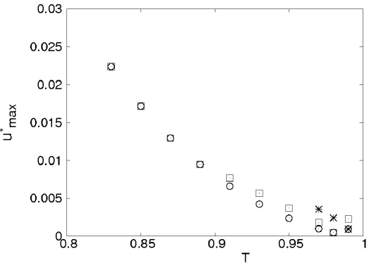
Figure 2: The maximum value of the spurious velocities for an equilibrated droplet is shown as a function of temperature $T$ for the SC case ($\ast$), the ODC case ($\Box$), and the OVC case ($\circ$) with $\kappa=0.3$ and $\tau=1$. Velocity is measured in units of $\Delta x/\Delta t$ and temperature in units of $T_{c}$.

The values of the maximum spurious velocities $u^{*}_{max}$ for the SC, ODC, and OVC cases are shown in Fig. 2 as a function of temperature. It appears that $u^{*}_{max}$ is minimized in the OVC case, as expected, and decreases when increasing the temperature. For this reason the OVC was preferred and adopted in the following.

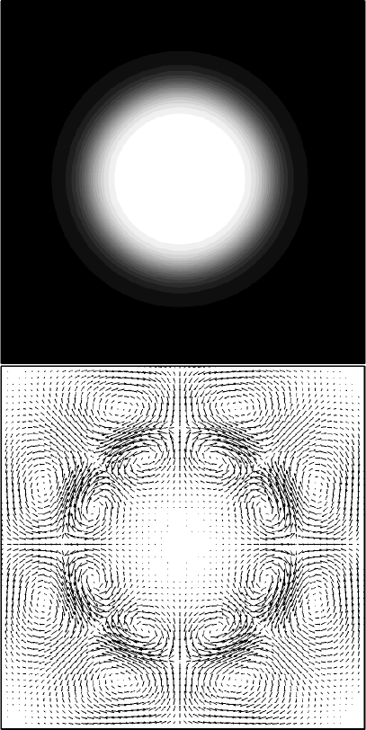
Figure 3: (Upper panel) The density contour of an equilibrated droplet with radius of 15 lattice units is shown for $\kappa=0.3$ and $\tau=1$ at $T=0.95$ in the OVC case. Grey-scaling from black $\rightarrow$ white corresponds to vapor $\rightarrow$ liquid. (Lower panel) The corresponding velocity pattern.

The equilibrium density pattern of the liquid droplet at $T=0.95$ with the corresponding velocity field is reported for the OVC case in Fig. 3. Velocities are not zero along the interface. The density profile across a section of the droplet is represented in Fig. 4 with an interface of about $6$ lattice spacings smoothly interpolating between the liquid and vapor states. The profile is well described by the approximate solution wagn07

$$n(x)=n_{V}^{th}+\frac{(n_{L}^{th}-n_{V}^{th})}{2}\Big{[}1+\tanh\Big{(}\frac{x}{\sqrt{2\kappa/(1/T-1)}}\Big{)}\Big{]}$$ (24)

of the equation $\partial_{\alpha}\Pi_{\alpha\beta}=0$.

A very nice feature of the present model is the independence of the phase diagram on the relaxation time $\tau$. To the best of our knowledge this was previously observed only in the model proposed in Ref. kupe09 , while variations in the equilibrium vapor density up to $50\%$ can be seen in the range $1\leq\tau\leq 2$ for other models shan93 ; he98 ; luo98 ; luo00 (see Fig. 2 of Ref. kupe09 ). This feature is illustrated in Fig. 5, where the equilibrium liquid and vapor densities at $T=0.95$ are shown, and holds also at different temperatures. Here we note that the optimal values $(N,Q)_{OVC}$ of Table 1 were not found depending on $\tau$. Finally, the behavior of $u^{*}_{max}$ as a function of $\tau$ for the same temperature is presented in Fig. 6 where a decrease with the relaxation time is observed.

IV Zebra phase and shear

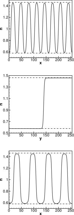
Figure 7: (Top) The density profile across the interface of the zebra phase for a periodic force with $A_{0}=10^{-4}$ and $\lambda=32$ in the case with $\tau=1$, $\kappa=0.3$ at $T=0.95$. The measured values for the density in the bulk are $n_{L}=1.459906$ and $n_{V}=0.580089$. Dashed lines represent the theoretical values $n_{L}^{th}$ and $n_{V}^{th}$ in a quiescent system without periodic potential at the same temperature (see the caption of Fig. 4). (Middle) The density profile along the $y$-direction at $x=L/2$ of a system under a periodic force with $A_{0}=10^{-4}$ and $\lambda=32$ and shear rate $\dot{\gamma}=10^{-3}$ (right bottom panel of Fig. 8). (Bottom) The density profile along the $x$-direction at $y=L/2$ of a system under a periodic force with $A_{0}=10^{-3}$ and $\lambda=64$ and shear rate $\dot{\gamma}=10^{-3}$ (right bottom panel of Fig. 10). Time is measured in units of $\Delta t$, lengths in units of $\Delta x$, and shear rate in units of $\Delta t^{-1}$.

In presence of the periodic force (7), a stable oscillating phase is found with the same period as in (7) and minimum and maximum values of density close to the vapor and liquid values at coexistence without external field, at the temperature under consideration, as shown in Fig. 7. This phase has been called zebra phase and a detailed study of the phase diagram has been done in Ref. Vink11 . An external flow is expected to distort the zebra order. We will consider a shear flow imposed by the top and bottom walls moving with opposite velocities $\pm\dot{\gamma}L_{y}/2$ along the $x$-direction. We will show in the following how the morphology of the zebra phase is affected by this flow. In a homogeneous system the shear would give the Couette profile ${\bf u^{*}}=(\dot{\gamma}(y-L_{y}/2),0)$, as it has been checked. The shear rate will be expressed in units of $\Delta t^{-1}$.

Figure 8 summarizes our results for the evolution of the zebra phase at different $\dot{\gamma}$ on a system of size $L_{x}\times L_{y}=256\times 256$ with $T=0.95$, $\tau=1$, and $\kappa=0.3$. The system is prepared through a quenching from a homogeneous state with symmetric composition at rest and shear is applied from the beginning of the simulations. The case with $\lambda=32$ and $A_{0}=10^{-4}$ is shown. At small values of shear the pattern is basically unaffected by the flow. At larger values of $\dot{\gamma}$ (middle row in Fig. 8) the zebra interfaces lose stability and at long times lamellae are destroyed. Liquid and vapor phases will coexist separated by an oblique interface that remains stable at times much larger than the last one in Fig. 8. Small ripples on this interface have the same periodicity of the external potential. When shear is further increased (see the case with $\dot{\gamma}=10^{-3}$) lamellae are destroyed sooner and a stationary state is observed with a single interface, in average aligned with flow, but with a superimposed oscillation (see the last snapshot on the right of the lower row of Fig. 8).

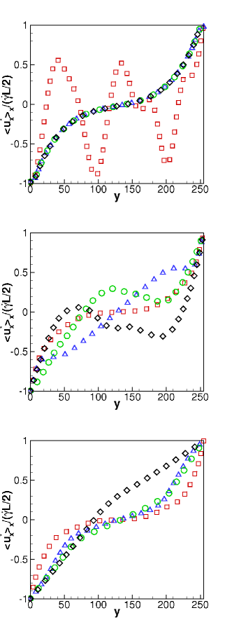
Figure 9: Profiles across the system of the $x$-component of the fluid velocity averaged along the $x$-direction of the patterns shown in Fig. 8 for $\dot{\gamma}=10^{-7},10^{-4},10^{-3}$ (from top to bottom) at $t=10^{3}$ (red squares), $10^{4}$ (blue triangles), $10^{5}$ (green circles), $2\times 10^{5}$ (black diamonds). The values of $|<u^{*}_{y}>_{x}|/(\dot{\gamma}L/2)$ are $\lesssim 0.05$ in all the cases. The maximum values of the spurious velocities are such that $u^{*}_{max}/(\dot{\gamma}L/2)\sim 10^{-4},10^{-4},10^{-2}$ from top to bottom. Time is measured in units of $\Delta t$, lengths in units of $\Delta x$, and shear rate in units of $\Delta t^{-1}$.

In all the cases of Fig. 8 shear becomes effective at times $t$ of order $10^{4}$. This time corresponds to the quantity $t_{S}=nL_{y}^{2}/(\eta\pi^{2})$ which is the leading contribution to the relaxation time for a shear flow in a simple fluid schl79 . The horizontally averaged component $<u^{*}_{x}>_{x}$ of the fluid velocity is shown in Fig. 9 at times corresponding to those of the snapshots in Fig. 8. Figure 9 shows that at the lower values of the shear rate ($\dot{\gamma}=10^{-7},10^{-4}$) a regular linear velocity profile is not formed (except close to the walls), even at the longest simulated time $t=10^{6}>>t_{S}$. On the contrary, at the highest value $\dot{\gamma}=10^{-3}$, the velocity profile along the flow direction shows a broken line. The slopes agree with those expected in a system with two phases of different density separated by a horizontal interface and given by $<u^{*}_{x}>_{x}/(\dot{\gamma}L_{y}/2)=4n_{u}y/[L_{y}(n_{u}+n_{l})]-1$ for $0\leq y\leq L_{y}/2$ and $<u^{*}_{x}>_{x}/(\dot{\gamma}L_{y}/2)=1-4n_{l}(L_{y}-y)/[L_{y}(n_{u}+n_{l})]$ for $L_{y}/2\leq y\leq L_{y}$ where $n_{l}$ and $n_{u}$ are the values of densities in the lower and upper half of the system, respectively papa99 .

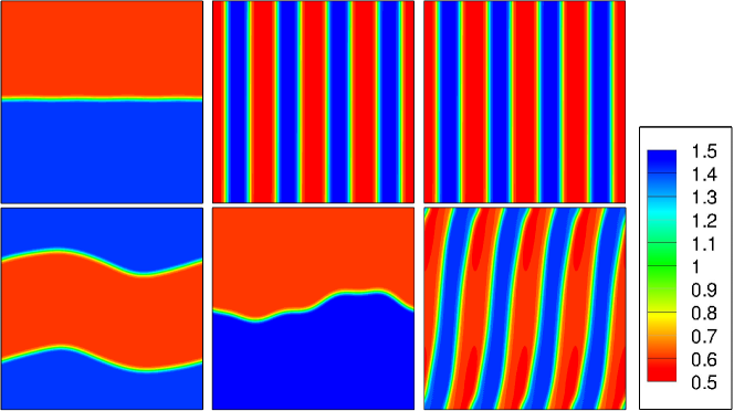
Figure 10: Late time density configurations for a system of size $256\times 256$ under a periodic force with $A_{0}=10^{-5},10^{-4},10^{-3}$ (from left to right) and $\lambda=64$ with shear rates $\dot{\gamma}=10^{-5}$ (upper row) and $\dot{\gamma}=10^{-3}$ (lower row). For the bulk values of the density see the comment in Fig. 8. Density values are depicted in the color bar at the right of the figure. Time is measured in units of $\Delta t$, lengths in units of $\Delta x$, and shear rate in units of $\Delta t^{-1}$.

By varying $\lambda$ and $A_{0}$, the pattern evolution, reported in Fig. 10, remains similar to that shown in Fig. 8. Lamellae with larger $\lambda$ are more stable against shear. For example, at $\dot{\gamma}=10^{-4}$ and $A_{0}=10^{-4}$ (not shown in Fig. 10), lamellae with $\lambda=64$ result only slightly distorted close to the walls and keep their periodicity, differently than in the case of Fig. 8 with $\lambda=32$ when they are destroyed by shear. Figure 10 also illustrates the role of different values of $A_{0}$. One observes, for example at $\dot{\gamma}=10^{-3}$, that the zebra phase remains stable at $A_{0}=10^{-3}$ while the fluid completely phase separates at $A_{0}=10^{-4}$.

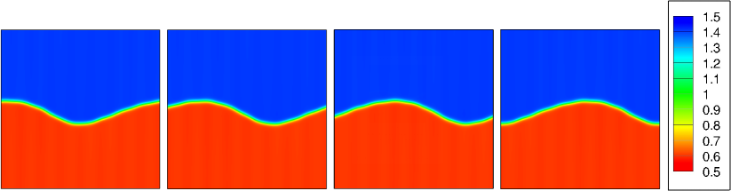
Figure 11: Density configurations at consecutive times $t=(4.90,4.92,4.94,4.96)\times 10^{5}$ (from left to right) for a system of size $256\times 256$ under a periodic force with $A_{0}=10^{-4}$, $\lambda=32$, shear rate $\dot{\gamma}=10^{-3}$. The bulk values of the density correspond to those reported in Fig. 4. Density values are depicted in the color bar at the right of the figure. Time is measured in units of $\Delta t$, lengths in units of $\Delta x$, and shear rate in units of $\Delta t^{-1}$.

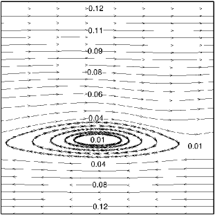
Figure 12: The velocity pattern with stream lines and velocity moduli at selected points corresponding to the third panel shown in Fig. 11. For this set of parameters the maximum value of spurious velocities is 0.002 (see Fig. 2). Velocities are measured in units of $\Delta x/\Delta t$.

In all the simulations at $T=0.95$, $\tau=1$, $A_{0}\leq 10^{-4}$, by increasing the shear rate, the density field was observed to behave as in the bottom right snapshot of Fig. 8. The nature of this state is better described in Fig. 11. It is a peculiar non-equilibrium state, characterized by a travelling wave on the liquid-vapor interface. It may be argued that at large shear, the oscillations induced by the periodic potential on the interface are advected by the flow resulting in the interface dynamics shown in Fig. 11. It is also interesting to see the behavior of the corresponding velocity pattern. This is plotted, for the third panel of Fig. 11, in Fig. 12 which clearly shows the existence of a recirculation flow field below the moving interface. The magnitude of the fluid velocity in such a pattern is about one order of magnitude larger than spurious currents measured for quiescent droplets thus confirming the physical origin of the observed structure. Such a vortex follows the interface wave and has been observed in all the cases where travelling waves appear as, for example, those with $A_{0}=10^{-4},10^{-5}$ and $\dot{\gamma}=10^{-3}$ in Fig. 10.

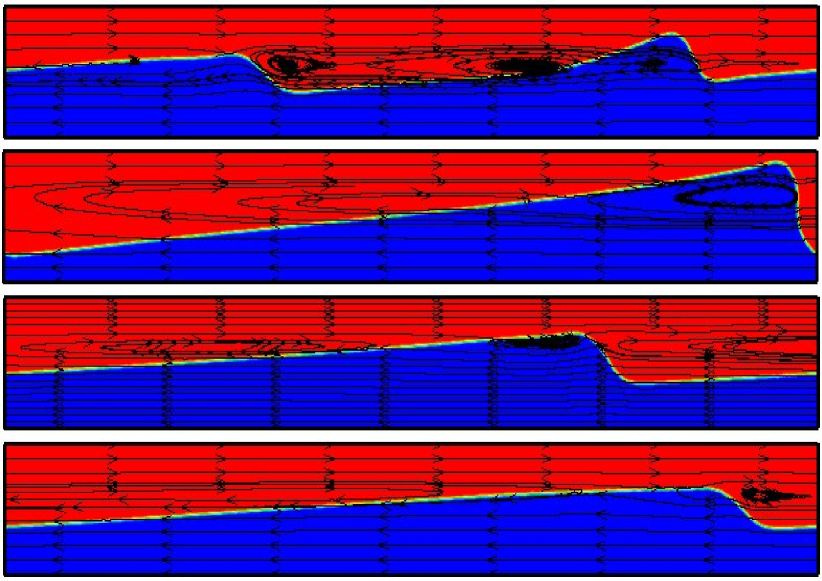
Figure 13: Density configurations with superimposed velocity patterns at times $t=(15,19,23,100)\times 10^{4}$ (from top to bottom) for a systems of size $2048\times 256$ under a periodic force with $A_{0}=10^{-4}$, $\lambda=32$, and shear rate $\dot{\gamma}=10^{-3}$. Density values are depicted in the color bar of Fig. 11. Time is measured in units of $\Delta t$, length in units of $\Delta x$, and shear rate in units of $\Delta t^{-1}$. Aspect ratio of frames is not preserved for a better view.

We deeply investigated if and how the wavelength and the amplitude of the observed wave would depend on the system parameters. As a first check, the length $L_{x}$ of the system was systematically increased assuming the values $512,1024,2048$ keeping the width $L_{y}=256$ fixed for the case shown in the lower row of Fig. 8. A single wave travelling over the whole system was always observed at long times. The evolution of the density patterns when $L_{x}=2048$, leading to the final configuration, is reported in Fig. 13 where the typical vortex structure of the flow field can be also appreciated. It is interesting to observe in this very long system the presence, in an intermediate time regime, of two different waves which later join into a single one indefinitely running over the system. Other simulations with different values of $\lambda,\tau,\kappa,T,A_{0},\dot{\gamma}$ (see below) confirmed the above pattern with a single wave, provided the shear rate is strong enough.

The amplitude $A$ of the interface wave, computed as the distance between the maximum and the minimum of the wave, was found to depend on the various parameters in a non trivial way. The stationary values of $A$ are reported in Table 2 for several cases. It results that the dependence of $A$ on the potential wavelength $\lambda$ and on the surface-tension parameter $\kappa$ is negligible. $A$ grows with the length $L_{x}$ of the system, saturating at the largest value of $L_{x}$, and with the shear rate $\dot{\gamma}$. On the contrary, we observe that $A$ decreases when increasing the relaxation time $\tau$, the potential amplitude $A_{0}$, and the temperature $T$. Actually, it was found that the interface wave survives down to $T=0.91$, where its amplitude is about a half of the system width, but dissolves for $T\leq 0.90$ where a flat horizontal interface separates liquid from vapor.

We also wanted to analyze the occurrence of the non-equilibrium state described above by using different initial conditions. We chose the most obvious initial state with a flat liquid-vapor interface parallel to the flow direction and studied the evolution of the system for different cases previously considered. We found the same behavior with a travelling wave as in Figs. 11-12 at large shear rates and we concluded that this picture is a general effect of the simultaneous presence of shear and periodic potential, independently of the choice of initial conditions. We also checked that the observed waves do not correspond to transient regimes. Indeed, the time evolution of the total interface length for systems of different sizes and initial conditions always shows a plateau at long times. On the other side, for $\dot{\gamma}\leq 10^{-4}$ (at $A_{0}=10^{-4}$ and $\lambda=32$), at large times, flat interfaces were found. We did not find evolutions resulting in oblique interfaces like those at $\dot{\gamma}=10^{-4}$ in Fig. 8. Therefore, differently than the case at larger shear rate, at small shear the stationary patterns depend on the initial state of the system.

Finally, we checked whether it would be possible to explain the presence of the interface waves as due to a sort of Kelvin-Helmholtz instability chan61 . This is an interface instability that may occur when two fluids with different density have different tangential velocities. By varying the shear rates or other parameters, we never observed the wave amplitude to grow making the interface unstable as in the Kelvin-Helmholtz instability that, we concluded, cannot be referred to our case.

V Conclusions

In this paper we have shown the effects of a shear flow on the density-oscillating “zebra” phase appearing in liquid-vapor systems in presence of a periodic potential. For this purpose, we have introduced a LBE with Gauss-Hermite quadrature in order to simulate van der Waals fluids. The advantages of this approach are that i) it is based on a systematic discretization of LBE, ii) spurious terms are avoided in the continuum equations (except for the $u^{*3}$ term in the Navier-Stokes equation), and iii) the equilibrium phase diagram does not depend on the relaxation time of the LBE. Higher isotropy derivatives have been considered in order to reduce spurious velocities. However, our results show that a larger reduction has been obtained by other approaches wagn07 ; nour02 .

We considered a region of the phase diagram where the “zebra” phase is stable. Shear was applied with flow perpendicular to the lamellae. Striped patterns with larger period or in a deeper potential, in general, were found less distorted by the flow. At high shear rates the “zebra” phase becomes unstable and the system completely separates into liquid and vapor regions. This state, however, is far from being trivial. It is characterized by travelling interface waves with steady total interface length at late times and by a recirculation pattern of the velocity field. Also in very large systems we always observed, at late times, a single perturbation moving over the lattice and one could ask about the origin of this behavior, in absence of any analytical proof of this instability. By increasing the length $L_{x}$, keeping fixed the other parameters, the energy injected into the system, due to the applied shear, increases with $L_{x}$. The increased amount of energy has to be organized in the velocity field and in the interface pattern and, in principle, more waves could also be expected. However, our results show that the injected energy always prefer to be organized in a single wave with the wavelength of the perturbation defined solely by the length $L_{x}$ of the channel. The corresponding velocity pattern is characterized by a single vortex - even if more waves and vortices are present at intermediate times. This behavior can be attributed to the fact that: 1. the external driving induces extended perturbations spanning over the whole system; 2. different waves, interacting each other, have an interfacial energy cost so that the coalescence into a single wave, when periodic boundary conditions (PBC) are applied, as shown in the sequence of configurations of Fig. 13, is reasonable. Since the use of PBC appears to be determinant in the above results, we also observe that the simulated system with periodic boundary conditions corresponds to consider a plane, normal to the symmetry axis, of the experimental setup (Couette cell) made of two co-axial counter-rotating cylinders.

Finally, we ask whether we can expect quantitative agreement between simulations and physical systems. We take the surface tension $\sigma$, the viscosity of the liquid phase $\eta_{L}$ and the interface width $\xi$ of the lattice Boltzmann (LB) model to correspond to the physical values via the relations $\xi^{LB}\Delta x^{ph}=\xi^{ph}$, $\sigma^{LB}\Delta m^{ph}/(\Delta t^{ph})^{2}=\sigma^{ph}$, and $\eta^{LB}\Delta m^{ph}/(\Delta t^{ph}\Delta x^{ph})=\eta^{ph}$. This defines physical length, time, and mass scales. In the case of mixtures of spherical silica colloids and PDMS polymers in solvent hoog99 $\sigma^{ph}=3\times 10^{-6}N/m$, $\eta_{L}^{ph}=0.097Pa\;s$, and $\xi^{ph}\simeq 10^{-8}m$. The interfacial thickness is about the size of the hydrodynamic radius of colloids and of the radius of gyration of polymers. For the values of $\xi^{LB},\sigma^{LB},\eta^{LB}$ used in the present paper, the physical scales are $\Delta x^{ph}=1.7\times 10^{-9}m$ and $\Delta t^{ph}=1.2\times 10^{-6}s$. With these values we can predict travelling waves to be observable at shear rates $\dot{\gamma}^{ph}=10^{-3}/\Delta t^{ph}=8.3\times 10^{2}s^{-1}$ with $\lambda^{ph}=64\Delta x^{ph}=1.1\times 10^{-7}m$ nota . We also expect that systems in $d=3$ will exhibit a still richer morphology but we leave this case for a future study.

$\;\;T$	$(N,Q)_{OVC}$	$(N,Q)_{ODC}$
0.83	(0.3,2.1)	(0.3,2.1)
0.85	(0.3,2.3)	(0.3,2.3)
0.87	(0.3,2.5)	(0.3,2.5)
0.89	(0.3,2.6)	(0.3,2.7)
0.91	(0.3,2.5)	(0.4,1.7)
0.93	(0.3,1.9)	(0.4,1.9)
0.95	(0.3,2.0)	(0.4,2.1)
0.97	(0.3,0.0)	(0.0,0.0)
0.98	(0.3,3.9)	(0.3,3.9)
0.99	(0.5,2.1)	(1.0,1.0)

Table 1: Optimal values of $N$ and $Q$ in (22)-(23) for the OVC and ODC cases with $\kappa=0.3$.

$\;\;T$	$\lambda$	$\tau$	$\dot{\gamma}$	$A_{0}$	$\kappa$	$L_{x}\times L_{y}$	$A/L_{y}$
0.95	32	1	$10^{-3}$	$10^{-4}$	0.3	$256\times 256$	0.172
0.95	64	1	$10^{-3}$	$10^{-4}$	0.3	$256\times 256$	0.172
0.95	32	1	$10^{-3}$	$10^{-4}$	0.3	$512\times 256$	0.316
0.95	64	1	$10^{-3}$	$10^{-4}$	0.3	$512\times 256$	0.316
0.95	32	1	$10^{-3}$	$10^{-4}$	0.3	$1024\times 256$	0.409
0.95	64	1	$10^{-3}$	$10^{-4}$	0.3	$1024\times 256$	0.409
0.95	32	1	$10^{-3}$	$10^{-4}$	0.3	$2048\times 256$	0.417
0.95	64	1	$10^{-3}$	$10^{-4}$	0.3	$2048\times 256$	0.417
0.95	32	1	$10^{-3}$	$10^{-5}$	0.3	$256\times 256$	0.178
0.95	64	1	$10^{-3}$	$10^{-5}$	0.3	$256\times 256$	0.178
0.95	32	1	$10^{-3}$	$10^{-5}$	0.3	$512\times 256$	0.335
0.95	64	1	$10^{-3}$	$10^{-5}$	0.3	$512\times 256$	0.335
0.95	32	1	$10^{-3}$	$10^{-5}$	0.3	$1024\times 256$	0.504
0.95	64	1	$10^{-3}$	$10^{-5}$	0.3	$1024\times 256$	0.504
0.95	32	1	$10^{-3}$	$10^{-4}$	0.2	$256\times 256$	0.172
0.95	32	1	$10^{-3}$	$10^{-4}$	0.5	$256\times 256$	0.172
0.95	32	2	$10^{-3}$	$10^{-4}$	0.3	$256\times 256$	0.112
0.95	64	2	$10^{-3}$	$10^{-4}$	0.3	$256\times 256$	0.112
0.95	32	2	$10^{-3}$	$10^{-4}$	0.3	$512\times 256$	0.219
0.95	64	2	$10^{-3}$	$10^{-4}$	0.3	$512\times 256$	0.219
0.95	32	3	$10^{-3}$	$10^{-4}$	0.3	$256\times 256$	0.00782
0.95	64	3	$10^{-3}$	$10^{-4}$	0.3	$256\times 256$	0.0234
0.95	32	3	$10^{-3}$	$10^{-4}$	0.3	$512\times 256$	0.166
0.95	64	3	$10^{-3}$	$10^{-4}$	0.3	$512\times 256$	0.166
0.91	32	1	$10^{-3}$	$10^{-4}$	0.3	$256\times 256$	0.255
0.91	64	1	$10^{-3}$	$10^{-4}$	0.3	$256\times 256$	0.255
0.91	32	1	$10^{-3}$	$10^{-4}$	0.3	$512\times 256$	0.397
0.91	64	1	$10^{-3}$	$10^{-4}$	0.3	$512\times 256$	0.397
0.91	32	1	$10^{-3}$	$10^{-4}$	0.3	$1024\times 256$	0.496
0.91	64	1	$10^{-3}$	$10^{-4}$	0.3	$1024\times 256$	0.496

Table 2: The amplitude $A$ of interface waves is reported for different system parameters.

Figure 1: The equilibrium phase diagram in the plane $(n,T)$ is shown for the SC case ($\ast$), the ODC case ($\Box$), and the OVC case ($\circ$) with $\kappa=0.3$ and $\tau=1$. Temperature and density are expressed in units of the critical values. The continuous line represents the theoretical prediction obtained from the Maxwell construction. Temperature and density are measured in units of $T_{c}$ and $n_{c}$, respectively.

Figure 4: The density profile across the interface of the droplet of Fig. 3. The line represents the prediction (24). The measured values for density in the bulk are $n_{L}=1.462721$ and $n_{V}=0.580015$ to be compared with the theoretical values $n_{L}^{th}=1.461727$ and $n_{V}^{th}=0.579015$. Density is measured in units of $n_{c}$ and space in units of $\Delta x$.

Figure 5: The equilibrium densities are shown as a function of the relaxation time $\tau$ for $\kappa=0.3$ at $T=0.95$ in the OVC case. Continuous lines are a guide to the eye. Density variations are less than $1\%$. Explicit values are given in Fig. 4. Density is measured in units of $n_{c}$ and time in units of $\Delta t$.

Figure 6: The maximum value of the spurious velocities for an equilibrated droplet is shown as a function of $\tau$ for $\kappa=0.3$ at $T=0.95$ in the OVC case. Velocity is measured in units of $\Delta x/\Delta t$ and time in units of $\Delta t$.

Figure 8: Density configurations at times $t=10^{3},10^{4},10^{5},2\times 10^{5}$ (from left to right) for a system of size $256\times 256$ under a periodic force with $A_{0}=10^{-4}$ and $\lambda=32$ with shear rates $\dot{\gamma}=10^{-7}$ (upper row), $\dot{\gamma}=10^{-4}$ (middle row), and $\dot{\gamma}=10^{-3}$ (lower row). The bulk values of density, when the zebra phase is stable, correspond to those without shear shown in the top panel of Fig. 7. When the zebra phase is destroyed, liquid and vapor density values correspond to the ones reported in Fig. 4. Density values are depicted in the color bar at the right of the figure. Time is measured in units of $\Delta t$, lengths in units of $\Delta x$, and shear rate in units of $\Delta t^{-1}$.

References

- (1) K. Binder, J. Horbach, R. L. C. Vink, and A. De Virgiliis, Soft Matter 4, 1555 (2008).
- (2) I. O. Götze, J. M. Brader, M. Schmidt, and H. Löwen, Mol. Phys. 101, 1651 (2003).
- (3) R. L. C. Vink, T. Neuhaus, and H. Löwen, J. Chem. Phys. 134, 204907 (2011).
- (4) R. L. C. Vink and A. J. Archer, Phys. Rev. E 85, 031505 (2012).
- (5) H. Gau, S. Herminghaus, P. Lenz, R. Lipowsky, Science 283, 46 (1999).
- (6) See, e. g., W. C. K. Poon, J. Phys.: Condens. Matter 14, R859 (2002).
- (7) A. K. Gunstensen, D. H. Rothman, S, Zaleski, and G. Zanetti, Phys. Rev. A 43, 4329 (1991).
- (8) D. Grunau, S. Chen, and K. Eggert, Phys. Fluids A 5, 2557 (1993).
- (9) X. Shan and H. Chen, Phys. Rev. E 47, 1815 (1993).
- (10) X. Shan and H. Chen, Phys. Rev. E 49, 2941 (1994).
- (11) X. Shan, Phys. Rev. E 73, 047701 (2006).
- (12) P. Yuan and L. Schaefer, Phys. Fluids 18, 042101 (2006).
- (13) M. Sbragaglia, R. Benzi, L. Biferale, S. Succi, K. Sugiyama, and F. Toschi, Phys. Rev. E 75, 026702 (2007).
- (14) M. Sbragaglia, R. Benzi, L. Biferale, H. Chen, X. Shan, and S. Succi, J. Fluid Mech. 628, 299 (2009).
- (15) G. Falcucci, G. Bella, G. Chiatti, S. Chibbaro, M. Sbragaglia, and S. Succi, Commun. Comput. Phys. 2, 1071 (2007).
- (16) X. Shan, Phys. Rev. E 77, 066702 (2008).
- (17) J. Zhang and F. Tian, Europhys. Lett. 81, 66005 (2008).
- (18) J. Hyvaluoma and J. Harting, Phys. Rev. Lett. 100, 246001 (2008).
- (19) A. L. Kupershtokh, D. A. Medvedev, and D. I. Karpov, Comput. Math. Appl. 58, 965 (2009).
- (20) G. Falcucci, G. Chiatti, S. Succi, A. Kuzmin, and A. M. Mohamad, Phys. Rev. E 79, 056706 (2009).
- (21) M. Sbragaglia, H. Chen, X. Shan, and S. Succi, Europhys. Lett. 86, 24005 (2009).
- (22) C. Wang, A. G. Xu, G. C. Zhang, and Y. J. Li, Sci. China Ser. G 52, 1337 (2009).
- (23) Z. Yu and L.-S. Fan, Phys. Rev. E 82, 046708 (2010).
- (24) G. Falcucci, S. Ubertini, and S. Succi, Soft Matter 6, 4357 (2010).
- (25) M. Sbragaglia and X. Shan, Phys. Rev. E 84, 036703 (2011).
- (26) C. E. Colosqui, G. Falcucci, S. Ubertini, and S. Succi, Soft Matter 8, 3789 (2012).
- (27) Q. Li, K. H. Luo, and X. J. Li, Phys. Rev. E 86, 016709 (2012).
- (28) M. R. Swift, W. R. Osborn, and J. M. Yeomans, Phys. Rev. Lett. 75, 830 (1995).
- (29) M. R. Swift, E. Orlandini, W. R. Osborn, and J. M. Yeomans, Phys. Rev. E 54, 5041 (1996).
- (30) T. Inamuro, N. Konishi, and F. Ogino, Comput. Phys. Commun. 129, 32 (2000).
- (31) A. J. Briant, A. J. Wagner, and J. M. Yeomans, Phys. Rev. E 69, 031602 (2004).
- (32) A. J. Wagner, Phys. Rev. E 74, 056703 (2006).
- (33) A. J. Wagner and C. M. Pooley, Phys. Rev. E 76, 045702(R) (2007).
- (34) Q. Li, K. H. Luo, Y. J. Gao, and Y. L. He, Phys. Rev. E 85, 026704 (2012).
- (35) L.-S. Luo, Phys. Rev. Lett. 81, 1618 (1998).
- (36) X. He, S. Chen, and R. Zhang, J. Comput. Phys. 152, 642 (1999).
- (37) L.-S. Luo, Phys. Rev. E 62, 4982 (2000).
- (38) X. He and G. D. Doolen, J. Stat. Phys. 107, 309 (2002).
- (39) V. Sofonea, A. Lamura, G. Gonnella, and A. Cristea, Phys. Rev. E 70, 046702 (2004); A. Cristea, G. Gonnella, A. Lamura, and V. Sofonea, Math. Comput. Simulat. 72, 113 (2006).
- (40) G. Gonnella, A. Lamura, and V. Sofonea, Phys. Rev. E 76, 036703 (2007); G. Gonnella, A. Lamura, and V. Sofonea, Eur. Phys. J. - Spec. Top. 171, 181 (2009).
- (41) A. Cristea, G. Gonnella, A. Lamura, and V. Sofonea, Commun. Comput. Phys. 7, 350 (2010).
- (42) Y. Gan, A. Xu, G. Zhang, Y. Li, and H. Li, Phys. Rev. E 84, 046715 (2011); Y. Gao, A. Xu, G. Zhang, P. Zhang, and Y. Li, EPL 97, 44002 (2012); Y. Gan, A. Xu, G. Zhang, and Y. Li, Front. Phys. 7, 481 (2012).
- (43) P. C. Philippi, K. K. Mattila, D. N. Siebert, L. O. E. dos Santos, L. A. Hegele Jr., and R. Surmas, J. Fluid Mech. 713, 564 (2012).
- (44) X. He, X. Shan, and G. D. Doolen, Phys. Rev. E 57, R13 (1998).
- (45) T. Lee and P. F. Fischer, Phys. Rev. E 74, 046709 (2006).
- (46) T. Lee and L. Liu, Phys. Rev. E 78, 017702 (2008).
- (47) T. Lee, Comput. Math. Appl. 58, 987 (2009).
- (48) T. Lee and L. Liu, J. Comput. Phys. 229, 8045 (2010).
- (49) D. Chiappini, G. Bella, S. Succi, F. Toschi, and S. Ubertini, Commun. Comput. Phys. 7, 423 (2010).
- (50) M. Gross, N. Moradi, G. Zikos, and F. Varnik, Phys. Rev. E 83, 017701 (2011).
- (51) G. Falcucci, S. Ubertini, D. Chiappini, and S. Succi, IMA J. Appl. Math. 76, 712 (2011).
- (52) Z. L. Guo, C. Zheng, and B. C. Shi, Phys. Rev. E 83, 036707 (2011).
- (53) Q. Lou, Z. L. Guo, and B. C. Shi, EPL 99, 64005 (2012).
- (54) X. Shan, X.-F. Yuan, and H. Chen, J. Fluid Mech. 550, 413 (2006).
- (55) Q. Li and A. J. Wagner, Phys. Rev. E 76, 036701 (2007).
- (56) J. S. Rowlinson and B. Widom, Molecular Theory of Capillarity, (Clarendon Press, Oxford, 1982).
- (57) J. Latt and B. Chopard, Math. Comput. Simulat. 72, 165 (2006).
- (58) R. Zhang, X. Shan, and H. Chen, Phys. Rev. E 74, 046703 (2006).
- (59) C. E. Colosqui, Phys. Rev. E 81, 026702 (2010).
- (60) Z. Guo, C. Zheng, and B. Shi, Phys. Rev. E 65, 046308 (2002).
- (61) A. Tiribocchi, N. Stella, G. Gonnella, and A. Lamura, Phys. Rev. E 80, 026701 (2009); G. Gonnella, A. Lamura, A. Piscitelli, and A. Tiribocchi, Phys. Rev. E 82, 046302 (2010).
- (62) G. Gonnella, A. Lamura, and A. Tiribocchi, Phil. Trans. R. Soc. A 369, 2592 (2011).
- (63) R. Evans, Adv. Phys. 28, 143 (1979).
- (64) R. R. Nourgaliev, T. N. Dinh, and B. R. Sehgal, Nucl. Eng. Des. 211, 153 (2002).
- (65) A. Lamura and G. Gonnella, Physica A 294, 295 (2001).
- (66) A. Tiribocchi, A. Piscitelli, G. Gonnella, and A. Lamura, Int. J. Numer. Method H. 21, 572 (2011).
- (67) C. M. Pooley and K. Furtado, Phys. Rev. E 77, 046702 (2008).
- (68) A. Cristea and V. Sofonea, Int. J. Mod. Phys. C 9, 1251 (2003).
- (69) A. J. Wagner, Int. J. Mod. Phys. B 17, 193 (2003).
- (70) A. L. Kupershtokh, Comput. Math. Appl. 59, 2236 (2010).
- (71) H. Schlichting, Boundary Layer Theory, (McGraw Hill, New York, 1979).
- (72) T. Papanastasiou, G. Georgiou, and A. Alexandrou, Viscous Fluid Flow, (CRC Press, Boca Raton, 1999).
- (73) S. Chandrasekhar, Hydrodynamic and Hydromagnetic Stability, (Oxford University, London, 1961).
- (74) E. H. A. de Hoog and H. N. W. Lekkerkerker, J. Phys. Chem. B 103, 5274 (1999).
- (75) Observe that, as well known yeo06 , it is not possible to choose all the variables to take the physical values still being able to perform stable and affordable runs since simulations of realistic experimental setups would require very large lattices (about nodes per direction!).
- (76) J. M. Yeomans, Physica A 369, 159 (2006).