Bell inequality and nonlocality in a two-dimensional mixed spin systems

Abstract

In this paper, we use Bell inequality and nonlocality to study the bipartite correlation in an exactly soluble two-dimensional mixed spin system. Bell inequality turns out to be a valuable detector for phase transitions in this model. It can detect not only the quantum phase transition, but also the thermal phase transitions, of the system. The property of bipartite correlation in the system is also analyzed. In the quantum anti-ferromagnetic phase, the Bell inequality is violated thus nonlocality is present. It is interesting that the nonlocality is enhanced by thermal fluctuation, and similar results have not been observed in anti-ferromagnetic phase. In the ferromagnetic phase, the quantum correlation turns out to be very novel, which cannot be captured by entanglement or nonlocality.

1 Introduction

Recently, quantum correlation in low-dimensional systems has attracted much attention. One the one hand, quantum correlation plays a central role in the formation of various condense matter phases at low temperatures. It helps us to understand these phases and the so-called quantum phase transitions(QPTs).[1] For example, for various models it has been found quantum correlation is maximum or singular in the vicinity of the transition points.[5, 4, 6, 2, 7, 3] On the other hand, quantum correlation is regarded as valuable resource for quantum information communication and quantum computation.[8, 9, 10]

The most famous features of quantum correlation are quantum entanglement and nonlocality. Entanglement is defined on the separability-entanglement paradigm.[10, 11] For example, the two-qubit pure state $|\uparrow_{1}\uparrow_{2}\rangle$ is separable, since it can be expressed as the product of the single-site states $|\uparrow_{1}\uparrow_{2}\rangle=|\uparrow_{1}\rangle\otimes|\uparrow_{2}\rangle$. However, most states cannot be expressed as such a product form, e.g., the superposition of two separable states $|\uparrow_{1}\uparrow_{2}\rangle+|\downarrow_{1}\downarrow_{2}\rangle$. They are called entangled states. The entanglement measurement is usually defined in the bipartite setting, such as entanglement concurrence and entanglement entropy. Recently, it has been recognized that entanglement can be generalized to multipartite settings.[12, 13]

Besides entanglement, nonlocality is also an important feature of quantum correlation, which is described by the violation of Bell inequalities[14, 15, 5, 16, 17]. We consider some expression $\mathcal{B}(\hat{\rho})$, namely, a function for the state $\hat{\rho}$. We will called it a Bell function. For all the states described by a realistic local theory, we can always identify the upper bound $\mathcal{B}_{0}$ for $\mathcal{B}(\hat{\rho})$. In other words, for any local state $\hat{\rho}$, it should hold

$$\mathcal{B}(\hat{\rho})\leq\mathcal{B}_{0}.$$

It is just a Bell inequality. For some state $\hat{\rho}$, suppose $\mathcal{B}(\hat{\rho})$ turns out to be larger than $\mathcal{B}_{0}$, we will say that the Bell inequality is violated, thus $\hat{\rho}$ cannot be characterized by any realistic local theory, i.e., $\hat{\rho}$ is a non-local state. A widely used Bell inequality is proposed by Clauser, Horne, Shimony and Holt, namely, the CHSH inequality.[18] Theoretically, numerical optimization can be used to identify the upper bound $\mathcal{B}_{0}$. Fortunately, a closed analytical formula of the Bell inequality for two-qubit states has been found by Horodecki.[19]

Nonlocality and entanglement were regarded as similar concepts for years. However, an entangled state may not violate any Bell inequality.[20, 21] For example, for several matrix product states, we found that the two-qubit states do not violate Bell inequality but they are entangled.[22] Thus, nonlocality and entanglement capture different aspects of quantum correlation. In fact, there even exists some kind of quantum correlation, which cannot be characterized by nonlocality and entanglement, as we will show in this paper. Quite recently, it has been found that Bell function can be used to indicate QPTs for many one-dimensional quantum systems.[6] It is interesting that it even can be used for topological QPT[3, 23] and Kosterlitz-Thouless QPT[5], which are difficult to capture by traditional order parameters.

Previous studies about Bell inequality and nonlocality are limited to QPTs in one-dimensional systems. Surprisingly, for various systems it turns out that the Bell inequality is not violated.[5, 6] It is recently realized that such an unexpected result is related to the monogamy trade-off obeyed by bipartite Bell function. As a result, in translation invariant systems, nonlocality should not be violated in general.[24] Based on this consideration, two-dimensional systems would be more suitable for preparing and then studying nonlocality. Firstly, two-dimensional systems have complex topology and a perfect translation-invariance symmetry is usually absent. Thus, the nonlocality can be present in the systems. Secondly, two-dimensional systems undergo not only QPTs at zero temperature, but also thermal phase transitions at finite temperatures. The study of nonlocality in thermal phase transitions would of course increase our understanding of quantum correlation and phase transitions.

In this paper, we will study Bell inequality and nonlocality in a two-dimensional Heisenberg-Ising mixed spin system.[25] Firstly, it is exactly soluble, thus we can concentrate on physics rather than mathematical calculation. Secondly, the model has a rich phase diagram. At zero temperature the system has an ferromagnetic (FM) phase and a quantum anti-ferromagnetic (QAF) phase, and a first-order QPT happens between the two phases. At finite temperatures, ordered ground states will be destroyed by thermal fluctuation, and the system will enter the paramagnetic (PM) phase. As a result, the system will undergo second-order thermal phase transition from the ordered magnetic phases to PM phase at finite temperatures. The phase diagram of the model is firstly identified by investigating the spin-spin correlation functions.[25] Recently, the system is investigated with the help of modern quantum information tools,[26, 27] and some issues remain unresolved. In the FM phase quantum entanglement turns out to be absent, however, quantum correlation is found to be present, indicated by the discord (discord measures all the quantum correlation in a quantum state).[26, 9] It is natural to ask, what is the intuitive form of the quantum correlation in the FM phase of the model? Can it be characterized by nonlocality? This is another motivation for us to investigate the nonlocality in this model.

This paper is organized as follows. In Sec. 2, we briefly introduce the model and basic formula. In Sec. 3, we study the relationship between Bell function and various phase transitions in the model. In Sec. 4, we discuss the properties of bipartite correlation in the system by analyzing nonlocality and other measures such as entanglement. A summary is given in Sec. 5.

2 Basic formula

2.1 Horodecki’s criterion

Firstly, let’s introduce Horodecki’s criterion [19] for nonlocality, which provides a closed analytic expression for the Bell inequality for any two-qubit state $\hat{\rho}$. We defines a matrix $\hat{\mathcal{L}}$ as

$$\mathcal{L}_{ij}(\hat{\rho})=\textrm{Tr}[\hat{\rho}\cdot\hat{\sigma}_{i}\otimes\hat{\sigma}_{j}],$$ (1)

where $\hat{\sigma}_{1},\hat{\sigma}_{2},\hat{\sigma}_{3}$ are just Pauli matrices. Then one finds the two largest eigenvalues of $\hat{\mathcal{L}}^{T}\hat{\mathcal{L}}$, denoted by $\lambda_{1}$ and $\lambda_{2}$. Finally, for any state described by a realistic local theory, the Bell inequality reads

$$\mathcal{B}(\hat{\rho})=2\sqrt{\lambda_{1}+\lambda_{2}}\leq 2.$$ (2)

Though the mathematical procedure seems to be complex, $\mathcal{B}(\hat{\rho})$ can be obtained analytically for any given two-qubit state $\hat{\rho}$. As we will show, $\mathcal{B}(\hat{\rho})$ is just related to two correlation functions of the system.

2.2 concurrence

In order to characterize the properties of the bipartite correlation, we will further calculate the entanglement concurrence.[11] Concurrence describes the pairwise entanglement between the two sites. Firstly, one defines a matrix $\tilde{\rho}$ as $\tilde{\rho}=\hat{\sigma}_{y}\otimes\hat{\sigma}_{y}\hat{\rho}^{*}\hat{\sigma}_{y}\otimes\hat{\sigma}_{y}$, then the concurrence is $\mathcal{C}=\textrm{max}\{0,\mu_{1}-\mu_{2}-\mu_{3}-\mu_{4}\}$, where $\mu_{i}$ are the square roots of the eigenvalues of the matrix $\hat{\rho}\tilde{\rho}$ in decreasing order. One can easily prove that the concurrence for the state $|\uparrow_{1}\uparrow_{2}\rangle$ is zero, i.e., it is separable, while the concurrence for the state $|\uparrow_{1}\uparrow_{2}\rangle+|\downarrow_{1}\downarrow_{2}\rangle$ is $1$, i.e., it is maximally entangled.

2.3 Model

We consider an exactly soluble two-dimensional mixed spin model firstly considered by J. Strecka.[25] The lattice (see Fig. 1) contains two kinds of spins: the Ising spins $\mu$ and the Heisenberg spins $S$, denoted by white dots and black dots, respectively. Four continuous spins forms a bond, labeled by $k$, and different bonds are connected with each other by the Ising spins. The two adjacent Heisenberg spins on bond $k$ have typical anisotropic Heisenberg interaction $-J(\Delta S_{k1}^{x}S_{k2}^{x}+\Delta S_{k1}^{y}S_{k2}^{y}+S_{k1}^{z}S_{k2}^{z})$, with $J$ the coupling parameter and $\Delta$ the anisotropy parameter, and the adjacent Heisenberg and Ising spins of bond $k$ have an Ising type interaction, i.e., $-J_{1}S_{k1}^{z}\mu_{k1}^{z}$. Finally, the totally Hamiltonian of the system is given by

$$\begin{array}[]{ccl}H&=&-J\sum_{k}(\Delta S_{k1}^{x}S_{k2}^{x}+\Delta S_{k1}^{y}S_{k2}^{y}+S_{k1}^{z}S_{k2}^{z})\\ &&-J_{1}\sum_{k}(S_{k1}^{z}\mu_{k1}^{z}+S_{k2}^{z}\mu_{k2}^{z})\end{array}$$ (3)

where the summation is over all bonds.

At zero temperature the system has two phases, i.e., a QAF phase and an FM phase, and a first-order phase transition separates the two from each other. The phase boundary is located at $J_{1c}=\frac{\Delta^{2}-1}{2}J$.[25] At finite temperatures, the system undergoes a second-order phase transition from the QAF phase to the paramagnetic (PM) phase for $J_{1}<J_{1c}$. While for $J_{1}>J_{1c}$, an FM-PM thermal phase transition will be observed. In this paper, the parameters are set as $J=1$ and $\Delta=2$, thus the QPT is located at $J_{1c}=1.5$.

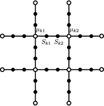
Figure 1: The topology of the two-dimensional mixed spin model.

We just pay our attention to the two adjacent Heisenberg spins on a bond, in which quantum correlation is present. Because of the symmetries of the system, the reduced density matrix $\hat{\rho}$ of the two-spin subsystem should be expressed as:[29]

$$\hat{\rho}=\left(\begin{array}[]{cccc}u_{+}&0&0&0\\ 0&v_{+}&z&0\\ 0&z&v_{-}&0\\ 0&0&0&u_{-}\end{array}\right),$$ (4)

where

$$\begin{array}[]{ccl}u_{\pm}&=&\frac{1}{4}\pm M_{z}+q_{zz}\\ v_{\pm}&=&\frac{1}{4}\pm\delta S_{z}-q_{zz}\\ z&=&2q_{xx}\end{array},$$ (5)

with $M_{z}=\frac{1}{2}\langle S_{1z}+S_{2z}\rangle$,$\delta S_{z}=\frac{1}{2}\langle S_{1z}-S_{2z}\rangle$,$q_{zz}=\langle S_{1z}S_{2z}\rangle$ and $q_{xx}=\langle S_{1x}S_{2x}\rangle$. According to Horodecki’s formula, the Bell inequality turns out to be

$$\mathcal{B}(\hat{\rho})=\max\{N_{1},N_{2}\}\leq 2$$ (6)

with $N_{1}=8\sqrt{q_{zz}^{2}+q_{xx}^{2}}$ and $N_{2}=8\sqrt{2q_{xx}^{2}}$.

Finally, to obtain the Bell function, one just needs to evaluate $q_{zz}$ and $q_{xx}$. Based upon the well-known existing results for two-dimensional Ising model, the solution of $q_{zz}$ and $q_{xx}$ involves Kambe projection method, the transfer matrix theory and several powerful spin identities. The calculation is rather lengthy. Readers who are interested in the method can read J. Strecka’s paper.[25] Here we just give the final results as follows

$$\begin{array}[]{ccc}q_{xx}&=&\frac{K_{1}+K_{2}}{8}+\frac{K_{1}-K_{2}}{2}\cdot q_{\mu\mu}\\ q_{zz}&=&\frac{K_{3}+K_{4}}{8}+\frac{K_{3}-K_{4}}{2}\cdot q_{\mu\mu}\end{array},$$ (7)

where $q_{\mu\mu}$ is just the spin-spin correlation function of the classical two-dimensional Ising model, which can be found on J. Strecka’s paper and the corresponding references.[25] The coefficients $K_{i}$ are given by

$$\begin{array}[]{cll}K_{1}&=&\frac{\sinh(\beta\frac{1}{2}J\Delta)}{e^{\frac{\beta J}{2}}\cosh\frac{\beta J_{1}}{2}+\cosh(\beta\frac{1}{2}J\Delta)}\\ K_{2}&=&\frac{\sinh(\beta\frac{1}{2}\sqrt{J_{1}^{2}+J^{2}\Delta^{2}})}{e^{\frac{\beta J}{2}}+\cosh(\beta\frac{1}{2}\sqrt{J_{1}^{2}+J^{2}\Delta^{2}})}\cdot\frac{J\Delta}{\sqrt{J_{1}^{2}+J^{2}\Delta^{2}}}\\ K_{3}&=&\frac{\cosh\frac{\beta J_{1}}{2}-e^{-\frac{\beta J}{2}}\cosh(\beta\frac{1}{2}J\Delta)}{\cosh\frac{\beta J_{1}}{2}+e^{-\frac{\beta J}{2}}\cosh(\beta\frac{1}{2}J\Delta)}\\ K_{4}&=&\frac{e^{\frac{\beta J}{2}}-\cosh(\beta\frac{1}{2}\sqrt{J_{1}^{2}+J^{2}\Delta^{2}})}{e^{\frac{\beta J}{2}}+\cosh(\beta\frac{1}{2}\sqrt{J_{1}^{2}+J^{2}\Delta^{2}})}\end{array}.$$ (8)

3 Bell function and phase transitions

In this section, we discuss the ability of Bell function in detecting the phase transitions in the model.

Firstly, we consider the QPT of the system. At zero temperature (and low temperatures), the system is in the QAF phase for $J_{1}<1.5$, and in the FM phase for $J_{1}>1.5$. In Fig. 2 we show the Bell function as a function of $J_{1}$ at $T=0.0015$. The Bell function shows a sudden-change at $J_{1}=1.5$. The discontinuity of $\mathcal{B}$ should result from the sudden-change of the density matrix, thus can be regarded as a reliable signal for a first-order phase transition. In addition, in the QAF phase, the value of the Bell function is larger than 2, thus the Bell inequality is violated. While in the FM phase, the Bell inequality is never violated.

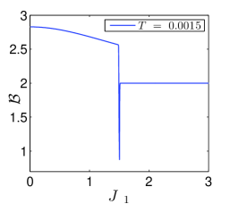
Figure 2: The Bell function $\mathcal{B}$ at $T=0.0015$. It shows a sudden-change at $J_{1}=1.5$.

Secondly, we study the behavior of the Bell function in the thermal phase transitions at finite temperature. The system has a QAF-PM transition for $J_{1}<1.5$, and an FM-PM transition for $J_{1}>1.5$. In Fig. 3 we show the temperature dependence of the Bell function in the QAF-PM transition. The derivative of $\mathcal{B}$ is divergent at some critical temperatures. Divergence of $\frac{\partial\mathcal{B}}{\partial T}$ should result from continuous and dramatic change of the density matrix, thus can be regarded as a reliable signal for second-order phase transitions. In fact, we have checked that the location of the divergence of the Bell function is indeed perfectly consistent with the divergent point of specific heat, thus the Bell function indeed identifies exactly the location of the thermal phase transition. In addition, in low-temperature region, the Bell function is larger than 2. Then, as the increase of the temperature, the Bell function decreases gradually. And finally, the Bell inequality is not violated at high-temperature regions. It shows that the nonlocality present at low temperatures is finally destroyed by thermal fluctuation.

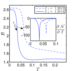
Figure 3: The behavior of Bell function in the QAF-PM thermal phase transition for several $J_{1}$. The Inset is the derivative of the Bell function with respect to the temperature. The derivative of Bell function is divergent at the critical temperature $T_{c}=0.035$ for $J_{1}=1.351$ and $T_{c}=0.063$ for $J_{1}=1.201$.

In Fig. 4 we plot the behavior of Bell function in the FM-PM thermal phase transition. Just as in the QAF-PM transition in Fig. 3, the derivative of $\mathcal{B}$ shows a divergence at the second-order phase transition point. In addition, the derivative of Bell function shows a discontinuity at $T_{0}=0.107$ for $J_{1}=1.802$ and $T_{0}=0.191$ for $J_{1}=2.102$. Detailed study manifests that it just results from the max function in calculating the Bell function, rather than a phase transition.

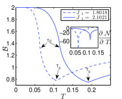
Figure 4: The behavior of Bell function in the FM-PM thermal phase transition for several $J_{1}$. The Inset is the derivative of the Bell function with respect to the temperature. The derivative of Bell function is divergent at the critical temperature $T_{c}=0.063$ for $J_{1}=1.802$ and $T_{c}=0.115$ for $J_{1}=2.102$.

In fact, according to Sec. 2, the Bell function is related to the spin-spin correlation functions as

$$\mathcal{N}=\max\{8\sqrt{q_{zz}^{2}+q_{xx}^{2}},8\sqrt{2q_{xx}^{2}}\}.$$ (9)

At the phase transition points, $q_{zz}$ or $q_{xx}$ can be singular. This is the mathematical reason why $\mathcal{N}$ can be used to detect the phase transitions in this model. It needs mention that the density matrix in Eq. (4) contains four free parameters $M_{z}$, $\delta S_{z}$, $q_{zz}$ and $q_{xx}$. The singularity of any of these four parameters would indicate a phase transition of the system. In fact, $M_{z}$ and $\delta S_{z}$ are just the traditional order parameters for the FM-PM and QAF-PM phase transitions, respectively. However, $\mathcal{N}$ just contains the information of $q_{zz}$ and $q_{xx}$. It needs mention that the concurrence is a function of $q_{zz}$, $q_{xx}$, and $M_{z}$, i.e., $\mathcal{C}=2\max\{0,2|q_{xx}|-\sqrt{(\frac{1}{4}+q_{zz})^{2}-M_{z}^{2}}\}$.[26] From a mathematical point of view, one may conclude that concurrence is better than the nonlocality in detecting phase transitions, since it contains more parameters in $\hat{\rho}$. However, it turns out that the concurrence $\mathcal{C}$ is zero in the FM-PM transition,[26] while $\mathcal{N}$ is just zero in a very narrow parameter space and it indeed offers a singularity at the critical temperature. Concurrence can only detect phase transitions in entangled states, while the Bell function can capture signals of phase transition in non-local states (Fig. 3) and local states (Fig. 4).

Furthermore, the max function in Eq. (9) induces a non-physical singularity, i.e., the discontinuity of $\frac{\partial\mathcal{N}}{\partial T}$ in Fig. 3. This kind of singularity should not be regarded as a reliable signal of phase transitions, since it can results from either the singularity of the density matrix, or merely the max function. Thus, if $\frac{\partial\mathcal{N}}{\partial T}$ turns out to be discontinuous in some models, we need to be very careful to judge whether it is a critical temperature or not. This kind of discontinuity has been observed in other measures of correlation such as concurrence and discord.[28, 26]

4 Properties of bipartite correlations

We calculate the Bell function and the concurrence in the $T-J_{1}$ plane, and the corresponding contour maps are shown in Fig. 5.

The figure shows that weaker coupling and lower temperature will result in higher quantum correlation in this model. One can see that high nonlocality or high entanglement is present in the bottom left corner of the maps. The effect of coupling constant on quantum correlation is model-dependent. Nevertheless, the relationship between temperature and quantum correlation is more general, because thermal fluctuation will destroy quantum correlation. From Fig. 5 one sees that for most $J_{1}$, as the temperature increases, both the nonlocality and concurrence will decrease gradually.

However, we find the nonlocality can be enlarged by thermal fluctuation in some parameter space. As indicated by the black arrow in Fig. 5, the contour line for $\mathcal{N}=2.8$ bends to the right. As a result, for an appropriate fixed $J_{1}$, for example $J_{1}=0.48$, when the temperature increases from zero, the Bell function will cross the $\mathcal{N}=2.8$ contour line from below, which means that the nonlocality is enhanced by thermal fluctuation. In the high-entanglement region in Fig. 5 (b), e.g., in the vicinity of the $\mathcal{C}=0.95$ contour line, the concurrence is not enhanced by thermal fluctuation. The different behavior between nonlocality and entanglement shows that the two concepts indeed capture different aspects of quantum correlation.

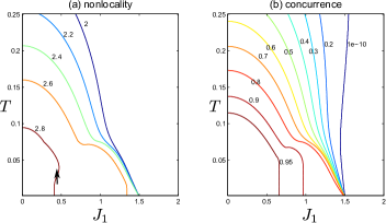
Figure 5: Contour maps for the (a) nonlocality and (b) concurrence in the $T-J_{1}$ plane.

In Fig. 6, we divide the $T-J_{1}$ plane into several regions by considering the form of bipartite correlation in the system. The red line is just the contour line for $\mathcal{N}=2$, on the left side of which the system is non-local. In addition, the blue line is the contour line of $\mathcal{C}=0$, on the left side of which the system is entangled. Finally, the whole $T-J_{1}$ plane is divided into three regions, labeled as $\mathrm{I}$, $\mathrm{II}$, $\mathrm{III}$. In region $\mathrm{I}$, both entanglement and nonlocality are present in the system. In region $\mathrm{II}$, the correlation is in the form of entanglement, rather than nonlocality. In region$\mathrm{III}$, where the FM-PM phase transition happens, there is no nonlocality or entanglement in the system. However, in a previous study,[26] we have found that quantum correlation is indeed present in the FM-PM phase transition by studying quantum discord. This result shows that the quantum correlation in region $\mathrm{III}$ is very novel, which cannot be characterized by entanglement or nonlocality. Quite recently, some other measures of bipartite correlation have been developed, for example, the so-called measure $Q$ for $2\times d$ systems.[30] These measures may offer further information about the quantum correlation in region $\mathrm{III}$.

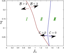
Figure 6: (Color Online) The $T-J_{1}$ plane is divided into three regions by analyzing the presence/absence of nonlocality and entanglement.

5 Summaries and discussions

In this paper, we have studied the bipartite correlation in a two-dimensional mixed spin system. We have used the Bell inequality to investigate the nonlocality in the system.

Firstly, Bell function captures the signals for both the quantum phase transition and thermal phase transitions of the model. In the vicinity of zero temperature, the Bell function $\mathcal{N}$ shows a sudden-change at the transition point $J_{1}=1.5$. In addition, at finite temperatures, $\frac{\partial\mathcal{N}}{\partial T}$ is divergent at the transition temperatures. The Bell function captures not just the location, but also the order, of these phase transitions.

Secondly, we find a novel type of quantum correlation, which cannot be characterized by entanglement or nonlocality. In region $\mathrm{III}$ of Fig. 6, the Bell inequality is not violated, and the concurrence is zero. However, a previous study shows that there is indeed quantum correlation present in the system.[26] Recently developed tools such as the measure $Q$ may be helpful to describe further physical picture for this kind of quantum correlation.[30]

Thirdly, we find the nonlocality can be enlarged by thermal fluctuation in the anti-ferromagnetic phase(see Fig. 3). As in-depth discussion is needed, let’s review several related papers first. In a one-dimensional diamond-like quantum spin model, the concurrence increases from $0$ to finite values when thermal fluctuation is increased gradually.[31] Similarly, for just the two-dimensional model studied in this paper, the discord, which is $0$ at zero temperature, is also enlarged by thermal fluctuation.[26] It needs mention that, in these two situations, the ground states are ferromagnetic, i.e. $|\uparrow\uparrow\uparrow...\rangle$, and all spins are parallel to each other, thus the quantum correlation is exactly zero at zero temperature. Then, as the increase of the temperature, excited states are mixed into the density matrix. These excited states are usually complicated, and it is expected for them to bring some quantum correlation into the system. That’s why thermal fluctuation can enhance correlation in ferromagnetic phases. However, our finding in this paper cannot be explained by the above picture. The ground state of the system is anti-ferromagnetic in the parameter space $J_{1}<J_{1c}$. Consequently, the system is in a highly non-local state. Thus the enhancement of nonlocality by thermal fluctuation in Fig. 3 is unusual. A possible approach to understand the behavior is to calculate low-lying states $|e_{i}\rangle$ explicitly, and analyze the mixing process $\sum_{i}e^{-\beta e_{i}}|e_{i}\rangle\langle e_{i}|\rightarrow\hat{\rho}$ as the change of the temperature. We’d like to mention that any qualitative discussion will be untenable, since the entanglement concurrence is not enlarged by the thermal fluctuation in the same parameter region. It suggests that quantum correlation phenomena, despite being extensively studied, is worthy of further investigation.

References

References

- [1] S. Sachdev, Quantum Phase Transitions, Cambridge University Press, 1999.
- [2] A.Osterloh, L. Amico, G. Falci, R. Fazio, Nature(London) 416 (2002) 608.
- [3] C. Castelnovo, and C. Chamon. Phys. Rev. B 77 (2008) 054433.
- [4] M.S. Sarandy, Phys. Rev. A 80 (2009) 022108.
- [5] L. Justino and Thiago R. de Oliveira, Phys. Rev. A 85 (2012) 052128.
- [6] Ferdi Altintas, Resul Eryigit. Annals of Physics 327 (2012) 3084.
- [7] Y.X. Chen, and S.W. Li, Phys. Rev. A 81 (2010) 032120.
- [8] Tarek A. Elsayed and Boris V. Fine, Phys. Rev. Lett. 110 ( 2013) 070404.
- [9] H. Ollivier, W.H. Zurek, Phys. Rev. Lett. 88 (2002) 017901.
- [10] K. Modi, T. Paterek, W. Son, V. Vedral, M. Williamson, Phys. Rev. Lett. 104 (2010) 080501
- [11] W.K. Wootters, Phys. Rev. Lett. 80 (1998) 2245.
- [12] Federico Levi and Florian Mintert, Phys. Rev. Lett. 110 (2013)150402.
- [13] Hui Li, Shuhao Wang, Jianlian Cui, and Guilu Long, Phys. Rev. A 87 (2013) 042335.
- [14] N. Gisin, Phys. Lett. A 154 (1991) 201.
- [15] X. G. Wang, Paolo Zanardi, Physics Letters A 301 (2002) 1.
- [16] J. S. Bell, Physics 1 (1964) 195.
- [17] R. F. Werner, Phys. Rev. A 40 (1989) 4277.
- [18] J.F. Clauser, M.A. Horne, A. Shimony, R.A. Holt , Phys. Rev. Lett. 23 (1969) 880.
- [19] R. Horodecki, P. Horodecki, M. Horodecki, Phys. Lett. A 200 (1995) 340.
- [20] J. Batle, and M. Casas, Phys. Rev. A 82 (2010) 062101 .
- [21] J Batle, and M Casas, J. Phys. A: Math. Theor. 44 (2011) 445304.
- [22] Hai-Lin Huang, Zhao-Yu Sun, and Bo Wang, Eur. Phys. J. B 86 (2013) 279.
- [23] D.L. Deng, C.F. Wu, J.L. Chen, S.J. Gu, S.X. Yu, C. H. Oh, arXiv:1111.4341v1.
- [24] Thiago R. de Oliveira, A. Saguia and M. S. Sarandy, Europhys. Lett. 100 (2012) 60004.
- [25] Jozef Strecka and Michal Jascur, Phys. Rev. B 66 (2002) 174415.
- [26] Z. Y. Sun, L. Li, N. Li, K. L. Yao, J. Liu, B. Luo, G. H. Du, and H. N. Li, Europhys. Lett. 95 (2011) 30008.
- [27] Wang Bo, Huang Hai-Lin, Sun Zhao-Yu, Kou Su-Peng, Chin. Phys. Lett. Vol. 29, No. 12 (2012) 120301.
- [28] M.F. Yang, Phys. Rev. A 71 (2005) 030302.
- [29] Luigi Amico and Andreas Osterloh, Francesco Plastina and Rosario Fazio, G. Massimo Palma, Phys. Rev. A 69 (2004) 022304.
- [30] Davide Girolami and Gerardo Adesso, Phys. Rev. Lett. 108 (2012) 150403.
- [31] Zhao-Yu Sun, Kai-Lun Yao, Wei Yao, De-Hua Zhang, and Zu-Li Liu, Phys. Rev. B 77 (2008) 014416.