Expurgated Random-Coding Ensembles: Exponents, Refinements and Connections

Abstract

This paper studies expurgated random-coding bounds and exponents for channel coding with a given (possibly suboptimal) decoding rule. Variations of Gallager’s analysis are presented, yielding several asymptotic and non-asymptotic bounds on the error probability for an arbitrary codeword distribution. A simple non-asymptotic bound is shown to attain an exponent of Csiszár and Körner under constant-composition coding. Using Lagrange duality, this exponent is expressed in several forms, one of which is shown to permit a direct derivation via cost-constrained coding which extends to infinite and continuous alphabets. The method of type class enumeration is studied, and it is shown that this approach can yield improved exponents and better tightness guarantees for some codeword distributions. A generalization of this approach is shown to provide a multi-letter exponent which extends immediately to channels with memory. Finally, a refined analysis expurgated i.i.d. random coding is shown to yield a $O\big{(}\frac{1}{\sqrt{n}}\big{)}$ prefactor, thus improving on the standard $O(1)$ prefactor. Moreover, the implied constant is explicitly characterized.

I Introduction

Achievable performance bounds for channel coding are typically obtained by analyzing the average error probability of an ensemble of codebooks with independently generated codewords. For memoryless channels, random codes with independent and identically distributed (i.i.d.) symbols achieve the channel capacity [1], characterize the error exponent of the best code at sufficiently high rates [2, Ch. 5], and provide tight bounds on the finite-length performance [3].

At low rates, the error probability of the best code in the random-coding ensemble can be significantly smaller than the average. In such cases, better performance bounds are obtained by considering an ensemble in which a subset of the randomly generated codewords are expurgated from the codebook. In particular, the error exponents resulting from such techniques are generally higher than the random-coding error exponent at low rates. Existing works exploring such techniques include those of Gallager [2, Sec. 5.7], Csiszár-Körner-Marton [4],[5, Ex. 10.18] and Csiszár-Körner [6]. The advantages of Gallager’s approach include its simplicity and the fact that the analysis is not restricted to finite alphabets. On the other hand, as we will see in Section III, the exponents of [6, 4, 5] can improve on that of Gallager for a given input distribution or decoding rule.

In this paper, we provide techniques that attain the best of each of the above approaches. Using variations of Gallager’s analysis, we obtain several asymptotic and non-asymptotic bounds for an arbitrary codeword distribution. Using these bounds, we provide derivations of both new and existing expurgated exponents, each yielding various advantages such as simplicity, generality, and guarantees of exponential tightness. We explore the method of type class enumeration (e.g. see [7, 8, 9]) for both discrete and continuous channels, and show that it can yield improved exponents and tightness guarantees, as well as providing a multi-letter exponent which extends immediately to channels with memory.

I-A System Setup

The input and output alphabets are denoted by $\mathcal{X}$ and $\mathcal{Y}$ respectively. The channel is assumed to be memoryless, yielding an $n$-letter transition law given by $W^{n}(\boldsymbol{y}|\boldsymbol{x})\triangleq\prod_{i=1}^{n}W(y_{i}|x_{i})$ for some conditional distribution $W(y|x)$. In the case that both $\mathcal{X}$ and $\mathcal{Y}$ are finite, the channel is a discrete memoryless channel (DMC), but we do not assume this to be the case in general. The encoder takes as input a message $m$ equiprobable on the set $\{1,\dotsc,M\}$, and transmits the corresponding codeword $\boldsymbol{x}^{(m)}$ from a codebook $\mathcal{C}=\{\boldsymbol{x}^{(1)},\dotsc,\boldsymbol{x}^{(M)}\}$. The decoder receives the vector $\boldsymbol{y}$ at the output of the channel, and forms the estimate

$$\hat{m}=\operatorname*{arg\,max}_{j\in\{1,\dotsc,M\}}q^{n}(\boldsymbol{x}^{(j)},\boldsymbol{y}),$$ (1)

where $q^{n}(\boldsymbol{x},\boldsymbol{y})\triangleq\prod_{i=1}^{n}q(x_{i},y_{i})$, and $q(x,y)$ is a non-negative function called the decoding metric. An error is said to have occurred if $\hat{m}\neq m$, and we assume that ties are broken as errors. We let $p_{e,m}(\mathcal{C})$ be the error probability induced by $\mathcal{C}$ given a particular message $m$, and we denote the maximal error probability by $p_{e}(\mathcal{C})\triangleq\max_{m}p_{e,m}(\mathcal{C})$.

When $q(x,y)=W(y|x)$, (1) is the optimal maximum-likelihood (ML) decoding rule. For other decoding metrics, this setting is that of mismatched decoding [10, 11, 12, 13], which is relevant when ML decoding is not feasible, e.g. due to channel uncertainty or implementation constraints.

Throughout the paper, we consider channels with both constrained and unconstrained inputs. In the former setting, each codeword $\boldsymbol{x}$ must satisfy a constraint of the form

$$\frac{1}{n}\sum_{i=1}^{n}c(x_{i})\leq\Gamma,$$ (2)

where $c(\cdot)$ is referred to as a cost function, and $\Gamma$ is a constant. Except where stated otherwise, it will be assumed that the input is unconstrained, which corresponds to $\Gamma=\infty$.

For a given rate $R$, an error exponent $E(R)$ is said to be achievable if there exists a sequence of codebooks $\mathcal{C}_{n}$ of length $n$ and rate $R$ whose error probability $p_{e}(\mathcal{C}_{n})$ satisfies

$$\liminf_{n\to\infty}-\frac{1}{n}\log p_{e}(\mathcal{C}_{n})\geq E(R).$$ (3)

We focus on the maximal error probability rather than the average error probability, but the two are equivalent for the purposes of studying error exponents.

I-B Previous Work

Considering ML decoding, Gallager [2, Ch. 5] studied an ensemble in which $2M-1$ codewords are generated at random, and a subset of $M$ codewords forms the codebook. Roughly speaking, the codewords which are kept are those which have the lowest error probability among the original codewords. A different approach was taken by Csiszár, Körner and Marton [4] (see also [5, Ex. 10.18]), who began by proving the existence of a collection of constant-composition codewords such that any two codewords have a joint empirical distribution satisfying certain properties. By analyzing this collection of codewords using the method of types, an error exponent was obtained which coincides with that of Gallager after the optimization of the input distribution. An exponent for mismatched decoding was derived by Csiszár and Körner [6], and was shown to coincide with that of [4] when particularized to the case of ML decoding.

As stated in the introduction, the exponents of [4, 6] can in fact improve on that of Gallager for a given input distribution. However, the proofs rely heavily on techniques which are valid only when the input and output alphabets are finite. In particular, [4] uses the type packing lemma [5, Ch. 10], and [6] uses a combinatorial graph decomposition lemma. For other related works, see [14, 15, 16, 17].

Overviews of the mismatched decoding problem can be found in [10, 11, 12, 13]. Most of the literature has focused on achievable rates, whereas this paper is concerned with the performance at low rates. The mismatched decoding paper most relevant to this one is [13], which studies random-coding error exponents for various non-expurgated ensembles.

I-C Contributions

The main contributions of this paper are as follows:

• In Section II, we present variations of Gallager’s analysis which yield several asymptotic and non-asymptotic bounds on the error probability. In particular, we consider the use of a logarithmic function in the expurgation argument in place of the power function used by Gallager [2, Sec. 7.3].

• In Section III, we present an overview of various expurgated exponents and the connections between them. Using the method of Lagrange duality [18], we relate the exponents given in [2, 4, 6]. Generalizations of the exponents in [2, 4] to the setting of mismatched decoding are given, and an alternative form of the exponent in [6] is given which extends readily to channels with infinite or continuous alphabets.

• In Section IV, we present several methods for deriving both new and existing exponents:

  • In Section IV-A, we present simple techniques for deriving exponents using a non-asymptotic bound from Section II. Applying constant-composition coding and the method of types recovers the exponent in [6], thus providing a simple and concise proof. Furthermore, applying cost-constrained coding with multiple auxiliary costs [13] recovers the generalization of this exponent to more general alphabets.

  • In Section IV-B, we study the method of type class enumeration (e.g. see [7, 8, 9]), which is shown to yield better exponents than the simpler approach for some codeword distributions, as well as better guarantees of exponential tightness.

  • In Section IV-C, we extend the type class enumeration analysis to allow for infinite and continuous alphabets. This is not only of interest in itself, but also yields a multi-letter exponent which can be directly applied to channels with memory and more general decoding metrics.

• In Section V, we present a refined derivation of Gallager’s exponent for i.i.d. random coding (and its generalization to mismatched decoding) with a $O\big{(}\frac{1}{\sqrt{n}}\big{)}$ prefactor, thus improving on the original $O(1)$ prefactor. Similar improvements for the non-expurgated random-coding error exponent have recently been obtained by Altuğ and Wagner [19] (see also [20]).

I-D Notation

We use bold symbols for vectors (e.g. $\boldsymbol{x}$), and denote the corresponding $i$-th entry using a subscript (e.g. $x_{i}$).

The set of all probability distributions on an alphabet, say $\mathcal{X}$, is denoted by $\mathcal{P}(\mathcal{X})$, and the set of all empirical distributions on a vector in $\mathcal{X}^{n}$ (i.e. types [5, Ch. 2]) is denoted by $\mathcal{P}_{n}(\mathcal{X})$. For a given type $Q\in\mathcal{P}_{n}(\mathcal{X})$, the type class $T^{n}(Q)$ is defined to be the set of all sequences in $\mathcal{X}^{n}$ with type $Q$.

The probability of an event is denoted by $\mathbb{P}[\cdot]$, and the symbol $\sim$ means “distributed as”. The marginals of a joint distribution $P_{XY}(x,y)$ are denoted by $P_{X}(x)$ and $P_{Y}(y)$. We write $P_{X}=\widetilde{P}_{X}$ to denote element-wise equality between two probability distributions on the same alphabet. Expectation with respect to a joint distribution $P_{XY}(x,y)$ is denoted by $\mathbb{E}_{P}[\cdot]$, or simply $\mathbb{E}[\cdot]$ when the associated probability distribution is understood from the context. Similarly, the mutual information with respect to $P_{XY}$ is written as $I_{P}(X;Y)$, or simply $I(X;Y)$ when the distribution is understood from the context. Given a distribution $Q(x)$ and conditional distribution $W(y|x)$, we write $Q\times W$ to denote the joint distribution defined by $Q(x)W(y|x)$.

For two positive sequences $f_{n}$ and $g_{n}$, we write $f_{n}\doteq g_{n}$ if $\lim_{n\to\infty}\frac{1}{n}\log\frac{f_{n}}{g_{n}}=0$, and we write $f_{n}\,\dot{\leq}\,g_{n}$ if $\limsup_{n\to\infty}\frac{1}{n}\log\frac{f_{n}}{g_{n}}\leq 0$, and analogously for $\dot{\geq}$. We write $f_{n}=O(g_{n})$ if $|f_{n}|\leq c|g_{n}|$ for some $c$ and sufficiently large $n$. All logarithms have base $e$, and all rates are in units of nats except in the examples, where bits are used. We define $[c]^{+}=\max\{0,c\}$, and denote the indicator function by $\leavevmode\hbox{\small 1\normalsize\kern-3.30002pt1}\{\cdot\}$.

II Expurgated Bounds

In this section, we present a number of variations of Gallager’s bounds and techniques which will provide the starting points of the derivations of the exponents in Section IV. We let $P_{\boldsymbol{X}}$ denote a codeword distribution, and we define the random variables $(\boldsymbol{X},\boldsymbol{Y},\overline{\boldsymbol{X}})$ distributed according to

$$(\boldsymbol{X},\boldsymbol{Y},\overline{\boldsymbol{X}})\sim P_{\boldsymbol{X}}(\boldsymbol{x})W^{n}(\boldsymbol{y}|\boldsymbol{x})P_{\boldsymbol{X}}({\overline{\boldsymbol{x}}}).$$ (4)

In the case that a cost constraint of the form (2) is present, we assume that $P_{\boldsymbol{X}}$ is chosen such that $\boldsymbol{X}$ satisfies the constraint with probability one.

We let $\mathsf{C}=\{\boldsymbol{X}^{(1)},\dotsc,\boldsymbol{X}^{(M^{\prime})}\}$ be a random codebook of size $M^{\prime}$ with each codeword independently generated according to $P_{\boldsymbol{X}}$. The symbol $\mathcal{C}$ is used to denote a fixed expurgated codebook containing $M\leq M^{\prime}$ codewords.

We begin with the following straightforward generalization of [2, Lemma, p. 151].

Lemma 1.

Fix a function $f\,:\,[0,1]\to\mathbb{R}$ and a codeword distribution $P_{\boldsymbol{X}}$ such that $f(p_{e,m}(\mathsf{C}))$ is non-negative for all $m$ with probability one. For any $\eta>0$, there exists a codebook $\mathcal{C}$ of size $M$ such that $M^{\prime}\frac{\eta}{1+\eta}<M\leq M^{\prime}$ and

$$f\big{(}p_{e,m}(\mathcal{C})\big{)}\leq(1+\eta)\mathbb{E}\big{[}f(p_{e,m}(\mathsf{C}))\big{]}$$ (5)

for $m=1,\dotsc,M$.

Proof.

The proof is identical to [2, Lemma, p. 151], with the assumption of $f(p_{e,m}(\mathsf{C}))$ being non-negative ensuring the validity of Markov’s inequality. ∎

While Lemma 1 is valid for any function $f(\cdot)$, it is primarily of interest when $f(\cdot)$ is monotonically increasing, so that (5) can be inverted in order to obtain an upper bound on $p_{e,m}(\mathcal{C})$. Gallager [2] presented the lemma with the choices $\eta=1$ and $f(\cdot)=(\cdot)^{1/\rho}$, where $\rho>0$, thus proving the existence of a codebook $\mathcal{C}$ of size $M$ such that

$$p_{e}(\mathcal{C})\leq\Big{(}2\mathbb{E}\big{[}p_{e,m}(\mathsf{C})^{1/\rho}\big{]}\Big{)}^{\rho},$$ (6)

where $\mathsf{C}$ contains $M^{\prime}=2M-1$ codewords. In the following theorem, we provide non-asymptotic bounds on the error probability which follow in a straightforward fashion from (6). The proof alters Gallager’s arguments for the purpose of better characterizing the non-asymptotic performance, and also for dealing with suboptimal decoding rules.

Theorem 1.

For any pair $(n,M)$, codeword distribution $P_{\boldsymbol{X}}$, and parameters $\rho\geq 1$ and $s\geq 0$, there exists a codebook $\mathcal{C}_{n}$ with $M$ codewords of length $n$ whose maximal error probability satisfies

$$p_{e}(\mathcal{C}_{n})\leq\mathrm{rcux}_{\rho}(n,M)\leq\mathrm{rcux}_{\rho,s}(n,M)$$ (7)

where

$$\mathrm{rcux}_{\rho}(n,M) \triangleq\bigg{(}4(M-1)\mathbb{E}\bigg{[}\mathbb{P}\Big{[}q^{n}(\overline{\boldsymbol{X}},\boldsymbol{Y})\geq q^{n}(\boldsymbol{X},\boldsymbol{Y})\,\Big{|}\,\boldsymbol{X},\overline{\boldsymbol{X}}\Big{]}^{1/\rho}\bigg{]}\bigg{)}^{\rho}$$ (8)

$$\mathrm{rcux}_{\rho,s}(n,M) \triangleq\Bigg{(}4(M-1)\mathbb{E}\Bigg{[}\mathbb{E}\Bigg{[}\bigg{(}\frac{q^{n}(\overline{\boldsymbol{X}},\boldsymbol{Y})}{q^{n}(\boldsymbol{X},\boldsymbol{Y})}\bigg{)}^{s}\,\Bigg{|}\,\boldsymbol{X},\overline{\boldsymbol{X}}\Bigg{]}^{1/\rho}\Bigg{]}\Bigg{)}^{\rho}.$$ (9)

Proof:

We obtain (8) from (6) by weakening the expectation as follows:

$$\mathbb{E}\big{[}p_{e,m}(\mathsf{C})^{1/\rho}\big{]} \leq\mathbb{E}\bigg{[}\bigg{(}\sum_{\overline{m}\neq m}\mathbb{P}\Big{[}q^{n}(\boldsymbol{X}^{(\overline{m})},\boldsymbol{Y})\geq q^{n}(\boldsymbol{X}^{(m)},\boldsymbol{Y})\,\Big{|}\,\boldsymbol{X}^{(m)},\boldsymbol{X}^{(\overline{m})}\Big{]}\bigg{)}^{1/\rho}\bigg{]}$$ (10)

$$\leq\mathbb{E}\bigg{[}2(M-1)\mathbb{P}\Big{[}q^{n}(\overline{\boldsymbol{X}},\boldsymbol{Y})\geq q^{n}(\boldsymbol{X},\boldsymbol{Y})\,\Big{|}\,\boldsymbol{X},\overline{\boldsymbol{X}}\Big{]}^{1/\rho}\bigg{]},$$ (11)

where (10) follows from the union bound, and (11) follows using $M^{\prime}=2M-1$ along with the inequality

$$\Big{(}\sum_{i}a_{i}\Big{)}^{1/\rho}\leq\sum_{i}a_{i}^{1/\rho},$$ (12)

which holds for any $\rho\geq 1$. We obtain (9) by applying Markov’s inequality to the inner probability in (8). ∎

Following the terminology of Polyanskiy et al. [3], we refer to the bounds in (8)–(9) as expurgated random-coding union (RCUX) bounds. These bounds are computable for sufficiently symmetric setups, and are thus of independent interest for characterizing the finite-length performance [3]. It should be noted that both $\mathrm{rcux}_{\rho}$ and $\mathrm{rcux}_{\rho,s}$ extend immediately to channels with memory and general decoding metrics (not necessarily single-letter).

The bound $\mathrm{rcux}_{\rho,s}$ was presented by Gallager [2] under ML decoding with $s=\frac{1}{2}$. For the random-coding ensembles we consider, it will be seen that this choice of $s$ is optimal for ML decoding, at least in terms of the error exponent. However, for mismatched decoding it is important to allow for an arbitrary choice of $s\geq 0$.

The following theorem gives an asymptotic bound which follows by using Lemma 1 with a choice of $f(\cdot)$ which differs from that of Gallager.

Theorem 2.

Consider a sequence of codebooks $\mathsf{C}_{n}$ containing $M_{n}^{\prime}=e^{nR}$ codewords which are generated independently according to $P_{\boldsymbol{X}}$. Suppose that there exists a non-negative sequence $E(n)$ growing subexponentially in $n$ (i.e. $E(n)\doteq 1$) such that

$$\mathbb{P}\big{[}q^{n}({\overline{\boldsymbol{x}}},\boldsymbol{Y})\geq q^{n}(\boldsymbol{x},\boldsymbol{Y})\,\big{|}\,\boldsymbol{X}=\boldsymbol{x}\big{]}\geq e^{-E(n)}$$ (13)

for all $\boldsymbol{x}$ and ${\overline{\boldsymbol{x}}}$ on the support of $P_{\boldsymbol{X}}$. Then there exists a sequence of codebooks $\mathcal{C}_{n}$ with $M_{n}$ codewords such that

$$\lim_{n\to\infty}\frac{1}{n}\log M_{n}=R$$ (14)

and

$$p_{e}(\mathcal{C}_{n}) \,\,\dot{\leq}\,\exp\Big{(}\mathbb{E}[\log p_{e,m}(\mathsf{C}_{n})]\Big{)}$$ (15)

$$\leq\exp\Big{(}\rho\,\mathbb{E}\Big{[}\log\mathbb{E}\big{[}p_{e,m}(\mathsf{C}_{n})^{1/\rho}\,\big{|}\,\boldsymbol{X}^{(m)}\big{]}\Big{]}\Big{)},$$ (16)

where (16) holds for any $\rho>0$.

Proof.

The error probability associated with the transmitted codeword $\boldsymbol{x}$ is lower bounded by the left-hand side of (13), where ${\overline{\boldsymbol{x}}}$ is any incorrect codeword. The assumption in (13) thus implies that the function $f(p_{e,m}(\mathsf{C}))=E(n)+\log p_{e,m}(\mathsf{C})$ is non-negative for $m=1,\dotsc,M$. Applying Lemma 1, we obtain that for each $n$ and any $\eta_{n}>0$ there exists a codebook $\mathcal{C}_{n}$ of size $M_{n}=e^{nR}\frac{\eta_{n}}{1+\eta_{n}}$ such that

$$E(n)+\log p_{e}(\mathcal{C}_{n})\leq(1+\eta_{n})\big{(}E(n)+\mathbb{E}[\log p_{e,m}(\mathsf{C}_{n})]\big{)}.$$ (17)

Since $\log\alpha\leq 0$ for $\alpha\in(0,1]$, it follows that

$$\log p_{e}(\mathcal{C}_{n})\leq\eta_{n}E(n)+\mathbb{E}[\log p_{e,m}(\mathsf{C}_{n})].$$ (18)

Choosing $\eta_{n}=\frac{1}{E(n)}$, we obtain (15), and the assumption that $E(n)\doteq 1$ implies (14). We obtain (16) by writing $\log\alpha=\rho\log(\alpha^{1/\rho})$, writing $\mathbb{E}[\,\cdot\,]=\mathbb{E}[\mathbb{E}[\,\cdot\,|\boldsymbol{X}^{(m)}]]$, and applying Jensen’s inequality. ∎

The assumption of Theorem 2 is mild, allowing ensembles for which the error probability associated with any two permissible codewords decays nearly double-exponentially fast. However, it is a multi-letter condition, and may therefore be difficult to verify directly. A single-letter sufficient condition depending only on the channel, metric and cost constraint (2) is that

$$\lim_{\gamma\to\infty}\frac{1}{\gamma}\log\log\frac{1}{\pi(\gamma)}=0,$$ (19)

where

$$\pi(\gamma) \triangleq\min_{(x,\overline{x})\,:\,c(x)\leq\gamma,c(\overline{x})\leq\gamma}\mathbb{P}[Y_{x}\in\mathcal{E}(x,\overline{x})]$$ (20)

$$\mathcal{E}(x,\overline{x}) \triangleq\big{\{}y\,:\,q(\overline{x},y)\geq q(x,y)\big{\}},$$ (21)

where in (20) we define $Y_{x}\sim W(\cdot|x)$. Under this assumption, the probability in (13) is lower bounded by the probability that $Y_{i}\in\mathcal{E}(X_{i},\overline{X}_{i})$ for $i=1,\dotsc,n$, which in turn is lower bounded by $\pi(n\Gamma)^{n}$. Since $n$ times a subexponential sequence is also subexponential, the condition of Theorem 2 follows from (19). Further discussion is given in Appendix A-A, along with some examples.

From (15), we can see the advantage of the expurgated ensemble over the non-expurgated one. The former yields the exponent corresponding to $-\frac{1}{n}\mathbb{E}[\log p_{e,m}(\mathsf{C}_{n})]$, which is higher in general than that of $-\frac{1}{n}\log\mathbb{E}[p_{e,m}(\mathsf{C}_{n})]$ due to Jensen’s inequality.

Using L’Hôpital’s rule, it is easily shown that $\lim_{\rho\to\infty}\rho\log\mathbb{E}[Z^{1/\rho}]=\mathbb{E}[\log Z]$ for any random variable $Z$. It follows that the inequality in (16) is actually an equality in the limit as $\rho\to\infty$. At first glance, it may appear that a similar argument can be used to show that (6) yields the same exponent as (15). However, there is an issue with the order of the limits of $n$ and $\rho$. If we take $\rho\to\infty$ in (6), the factor $2^{\rho}$ makes the right-hand side equal $\infty$. Letting $\rho$ grow slowly with $n$ is also potentially problematic, since the random variable $p_{e,m}(\mathsf{C})$ varies with $n$.

The bounds in Theorem 2 will prove useful for deriving improved exponents compared to Theorem 1 for some codeword distributions, and for extending the type class enumeration method beyond the finite-alphabet setting.

III Expurgated Ensembles and Exponents

In this section, we present an overview of various expurgated exponents and the connections between them. Our focus here is primarily on existing exponents or simple variations thereof, though we also provide a dual form of the exponent in [6] which is new to the best of our knowledge. Further exponents which appear for the first time in this paper are given in Theorems 5 and 7 in Section IV.

Throughout the paper, we consider three expurgated ensembles, each of which depends on an input distribution $Q$:

1. The i.i.d. ensemble is characterized by

   $$P_{\boldsymbol{X}}(\boldsymbol{x})=\prod_{i=1}^{n}Q(x_{i}).$$ (22)

   This codeword distribution is valid for both discrete and continuous alphabets, but it is not suitable for channels with cost constraints, since in all non-trivial cases there is a non-zero probability of violating the constraint.

2. The constant-composition ensemble is characterized by

   $$P_{\boldsymbol{X}}(\boldsymbol{x})=\frac{1}{|T^{n}(Q_{n})|}\leavevmode\hbox{\small 1\normalsize\kern-3.30002pt1}\big{\{}\boldsymbol{x}\in T^{n}(Q_{n})\big{\}},$$ (23)

   where $Q_{n}$ is a type with the same support as $Q$ such that $|Q_{n}(x)-Q(x)|=O\big{(}\frac{1}{n}\big{)}$ for all $x$. This codeword distribution relies on the input being finite. It is directly applicable to channels with cost constraints, since each codeword satisfies (2) provided that $\mathbb{E}_{Q_{n}}[c(X)]\leq\Gamma$, which in turn can be achieved provided that $\mathbb{E}_{Q}[c(X)]\leq\Gamma$.

3. The cost-constrained ensemble is characterized by

   $$P_{\boldsymbol{X}}(\boldsymbol{x})=\frac{1}{\mu_{n}}\prod_{i=1}^{n}Q(x_{i})\leavevmode\hbox{\small 1\normalsize\kern-3.30002pt1}\big{\{}\boldsymbol{x}\in\mathcal{D}_{n}\big{\}},$$ (24)

   where

   $$\mathcal{D}_{n}\triangleq\bigg{\{}\boldsymbol{x}\,:\,\frac{1}{n}\sum_{i=1}^{n}c(x_{i})\leq\Gamma,\bigg{|}\frac{1}{n}\sum_{i=1}^{n}a_{l}(x_{i})-\phi_{l}\bigg{|}\leq\frac{\delta}{n},\,l=1,\dotsc,L\bigg{\}},\\$$ (25)

   and where $\delta$ is a positive constant (independent of $n$), $\{a_{l}(\cdot)\}_{l=1}^{L}$ are functions with means $\phi_{l}\triangleq\mathbb{E}_{Q}[a_{l}(X)]$, and $\mu_{n}$ is a normalizing constant. This codeword distribution is valid for both discrete and continuous alphabets, and ensures that each codeword satisfies (2). Both $c(\cdot)$ and $\{a_{l}(\cdot)\}$ can be thought of as cost functions, and we will distinguish between the two by referring to them as the system cost and auxiliary costs respectively. In contrast to the system cost, the auxiliary costs are functions which can be optimized. That is, while the system cost is given as part of the problem statement, the auxiliary costs are introduced to improve the performance of the random-coding ensemble itself [12, 21, 13].

We proceed by stating and comparing the exponents obtained by the above ensembles; derivations will be given in Section IV. Except where stated otherwise, we assume that the channel is a DMC with unconstrained inputs.

A straightforward generalization of Gallager’s i.i.d. exponent to the setting of mismatched decoding is as follows:

$$E_{\mathrm{ex}}^{\mathrm{iid}}(Q,R)\triangleq\sup_{\rho\geq 1}E_{\mathrm{x}}^{\mathrm{iid}}(Q,\rho)-\rho R,$$ (26)

where

$$E_{\mathrm{x}}^{\mathrm{iid}}(Q,\rho)\triangleq\sup_{s\geq 0}-\rho\log\sum_{x,\overline{x}}Q(x)Q(\overline{x})\Bigg{(}\sum_{y}W(y|x)\bigg{(}\frac{q(\overline{x},y)}{q(x,y)}\bigg{)}^{s}\Bigg{)}^{1/\rho}.$$ (27)

The objective in (27) is concave in $s$, and under ML decoding (i.e. $q(x,y)=W(y|x)$), it is also unchanged when $s$ is replaced by $1-s$. From these properties, it follows that $s=\frac{1}{2}$ is optimal for ML decoding, and thus the exponent is the same as that of Gallager [2].

Csiszár and Körner [6] make use of the constant-composition codeword distribution in (23). The analysis is significantly different to that of Gallager, and yields an exponent in a different form, namely

$$E_{\mathrm{ex}}^{\mathrm{cc}}(Q,R)\triangleq\min_{\begin{subarray}{c}P_{X\overline{X}Y}\in\mathcal{T}(Q)\\ I_{P}(X;\overline{X})\leq R\end{subarray}}D(P_{X\overline{X}Y}\|Q\times Q\times W)-R,$$ (28)

where the notation $Q\times Q\times W$ denotes the distribution $Q(x)Q(\overline{x})W(y|x)$, and

$$\mathcal{T}(Q)\triangleq\Big{\{}P_{X\overline{X}Y}\in\mathcal{P}(\mathcal{X}\times\mathcal{X}\times\mathcal{Y})\,:\,P_{X}=Q,P_{\overline{X}}=Q,\mathbb{E}_{P}[\log q(\overline{X},Y)]\geq\mathbb{E}_{P}[\log q(X,Y)]\Big{\}}.$$ (29)

The objective in (28) follows from [6, Eq. (32)] and the identity

$$D(P_{X\overline{X}Y}\|Q\times Q\times W)=D(P_{X\overline{X}Y}\|P_{X\overline{X}}\times W)+I_{P}(X;\overline{X}),$$ (30)

which holds for any $P_{X\overline{X}Y}$ such that $P_{X}=P_{\overline{X}}=Q$. Defining $P_{Y}(y)\triangleq\sum_{x}Q(x)W(y|x)$, we observe that $E_{\mathrm{ex}}^{\mathrm{cc}}$ is positive for sufficiently small $R$ provided that $\mathbb{E}_{Q\times W}[\log q(X,Y)]>\mathbb{E}_{Q\times P_{Y}}[\log q(X,Y)]$. It was shown in [11] that the mismatched capacity is in fact zero unless this condition holds for some $Q$.

The following theorem provides the means for comparing the above two exponents, as well as that of [4].

Theorem 3.

For any input distribution $Q$ and rate $R$, we have

$$E_{\mathrm{ex}}^{\mathrm{cc}}(Q,R) =\sup_{s\geq 0}\min_{\begin{subarray}{c}P_{X\overline{X}}\,:\,P_{X}=Q,P_{\overline{X}}=Q,\\ I_{P}(X;\overline{X})\leq R\end{subarray}}\mathbb{E}_{P}[d_{s}(X,\overline{X})]+I_{P}(X;\overline{X})-R$$ (31)

$$=\sup_{\rho\geq 1}E_{\mathrm{x}}^{\mathrm{cc}}(Q,\rho)-\rho R,$$ (32)

where

$$d_{s}(x,\overline{x}) \triangleq-\log\sum_{y}W(y|x)\bigg{(}\frac{q(\overline{x},y)}{q(x,y)}\bigg{)}^{s}$$ (33)

$$E_{\mathrm{x}}^{\mathrm{cc}}(Q,\rho) \triangleq\sup_{s\geq 0,a(\cdot)}-\rho\sum_{x}Q(x)\log\sum_{\overline{x}}Q(\overline{x})\Bigg{(}\sum_{y}W(y|x)\bigg{(}\frac{q(\overline{x},y)}{q(x,y)}\bigg{)}^{s}\frac{e^{a(\overline{x})}}{e^{a(x)}}\Bigg{)}^{1/\rho}.$$ (34)

Proof:

See Appendix A-B. ∎

Equations (32) and (34) strongly resemble (26)–(27). Equation (31) is a generalization of the exponent in [4], which is recovered by setting $q(x,y)=W(y|x)$ and $s=\frac{1}{2}$. Using the same argument as the one following (27), it can be shown that the latter choice is optimal. From the proof of Theorem 3, this implies the optimality of $s=\frac{1}{2}$ in (34) under ML decoding, though the optimal choice of $a(\cdot)$ is unclear in general. To our knowledge, the expression in (34) has not appeared previously even for ML decoding.

As noted in [16, 6], we can write (31) in the language of rate-distortion theory [22, Ch. 10]. Fix $s\geq 0$ and define

$$D_{s}(Q,R)\triangleq\min_{\begin{subarray}{c}P_{X\overline{X}}\,:\,P_{X}=Q,P_{\overline{X}}=Q,\\ I_{P}(X;\overline{X})\leq R\end{subarray}}\mathbb{E}_{P}[d_{s}(X,\overline{X})].$$ (35)

This can be interpreted as the distortion-rate function of a source $X$ with a reproduction variable $\overline{X}$, subject to the additional constraint that each reproduction codeword ${\overline{\boldsymbol{x}}}$ has empirical distribution $Q$. For any $s\geq 0$, the constraint on the mutual information in (31) is active for sufficiently small $R$. The supremum of all such rates is given by

$$R_{s}(Q)\triangleq I_{P^{*}}(X;\overline{X}),$$ (36)

where

$$P_{X\overline{X}}^{*}\triangleq\operatorname*{arg\,min}_{P_{X\overline{X}}\,:\,P_{X}=Q,P_{\overline{X}}=Q}\mathbb{E}_{P}[d_{s}(X,\overline{X})]+I_{P}(X;\overline{X}).$$ (37)

For $R\leq R_{s}$ we have $I_{P}(X;\overline{X})=R$ under the minimizing $P_{X\overline{X}Y}$, whereas for $R\geq R_{s}$ the minimum in (31) decreases linearly with $R$ for any fixed $s$. It follows that

$$E_{\mathrm{ex}}^{\mathrm{cc}}(Q,R)=\sup_{s\geq 0}E_{\mathrm{ex}}^{\mathrm{cc}}(Q,R,s),$$ (38)

where

$$E_{\mathrm{ex}}^{\mathrm{cc}}(Q,R,s)\triangleq\begin{cases}D_{s}(Q,R)&R\leq R_{s}(Q)\\ D_{s}(Q,R_{s})+R_{s}(Q)-R&R>R_{s}(Q).\end{cases}$$ (39)

By applying Jensen’s inequality to (34) and setting $a(x)=0$, we immediately obtain

$$E_{\mathrm{ex}}^{\mathrm{cc}}(Q,R)\geq E_{\mathrm{ex}}^{\mathrm{iid}}(Q,R).$$ (40)

It was shown in [5, Ex. 10.18] that (40) holds with equality under ML decoding with an optimized input distribution $Q$. However, when either the decoding rule or input distribution is fixed, the inequality in (40) can be strict; an example is given at the end of this section. In Section IV-A, we show that the stronger exponent $E_{\mathrm{ex}}^{\mathrm{cc}}$, in the form given in (32), remains achievable in the case of continuous alphabets, with the summations in (34) replaced by integrals. This is proved using the cost-constrained ensemble in (24).

The following proposition generalizes Gallager’s expression for the expurgated exponent as $R\to 0^{+}$ for channels whose zero-error capacity [23] is zero, and shows that the inequality in (40) becomes an equality in the limit.

Proposition 1.

Fix any input distribution $Q$ such that all pairs $(x,\overline{x})$ with $Q(x)Q(\overline{x})>0$ share a common output, i.e. $W(y|x)W(y|\overline{x})>0$ for some $y$. Then

$$\lim_{R\rightarrow 0^{+}}E_{\mathrm{ex}}^{\mathrm{cc}}(Q,R)=\lim_{R\rightarrow 0^{+}}E_{\mathrm{ex}}^{\mathrm{iid}}(Q,R)=\sup_{s\geq 0}\mathbb{E}[d_{s}(X,\overline{X})],$$ (41)

where $d_{s}$ is defined in (33), and the expectation is taken with respect to $Q(x)Q(\overline{x})$.

Proof:

See Appendix A-C. ∎

We conclude this section with a numerical example. The channel is defined by the entries of the $|\mathcal{X}|\times|\mathcal{Y}|$ matrix

$$\left[\begin{array}[]{ccc}1-2\delta_{0}&\delta_{0}&\delta_{0}\\ \delta_{1}&1-2\delta_{1}&\delta_{1}\\ \delta_{2}&\delta_{2}&1-2\delta_{2}\end{array}\right],$$ (42)

and the decoding metric is defined similarly with a fixed $\delta\in(0,\frac{1}{3})$ in place of each $\delta_{i}$ ($i=1,2,3$), yielding a minimum Hamming distance rule. Figure 1 plots the exponents in the case that $\delta_{0}=0.01$, $\delta_{1}=0.05$, $\delta_{2}=0.25$ and $Q=\big{(}\frac{1}{3},\frac{1}{3},\frac{1}{3}\big{)}$. We observe that $E_{\mathrm{ex}}^{\mathrm{cc}}>E_{\mathrm{ex}}^{\mathrm{iid}}$ at all positive rates, and the gap is particularly significant in the mismatched case. However, consistent with Proposition 1, the two coincide in the limit as $R\to 0$.

As noted in [6], if $Q$ is optimized, then the two exponents coincide for ML decoding. However, the strict inequality $E_{\mathrm{ex}}^{\mathrm{cc}}>E_{\mathrm{ex}}^{\mathrm{iid}}$ remains possible for other decoding rules.

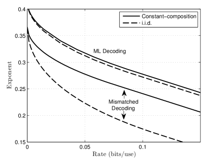
Figure 1: Expurgated exponents for the channel described in (42) with minimum Hamming distance decoding and ML decoding. The parameters are $\delta_{0}=0.01$, $\delta_{1}=0.05$, $\delta_{2}=0.25$ and $Q=\big{(}\frac{1}{3},\frac{1}{3},\frac{1}{3}\big{)}$

IV Derivations of the Expurgated Exponents

In this section, we provide several techniques for deriving the expurgated exponents, including those introduced in Section III and a further two in Theorems 5 and 7 below. The approaches given here have various advantages which were outlined in Section I-C, and which are discussed further in Section IV-D. Throughout the section, expectations are written using summations for notational simplicity (e.g. $\mathbb{E}_{Q}[f(X)]=\sum_{x}Q(x)f(x)$). However, we will highlight that certain results apply in the case of continuous alphabets upon replacing the summations by integrals.

IV-A Derivations Using Theorem 1

IV-A1 i.i.d. ensemble

We immediately obtain the exponent in (26), as well as its generalization to continuous alphabets, by substituting the i.i.d. distribution in (22) into $\mathrm{rcux}_{\rho,s}$ in (9).

IV-A2 Constant-composition Ensemble

In the case of finite alphabets, the method of types [5, Ch. 2] can be used to obtain the exact exponents corresponding to $\mathrm{rcux}_{\rho}$ and $\mathrm{rcux}_{\rho,s}$ for each of the ensembles defined in (22)–(24). The analysis is similar for each of these, so we focus on the constant-composition ensemble described by (23). We define

$$\mathcal{S}(Q) \triangleq\Big{\{}\widetilde{P}_{X\overline{X}}\in\mathcal{P}(\mathcal{X}\times\mathcal{X})\,:\,\widetilde{P}_{X}=Q,\widetilde{P}_{\overline{X}}=Q\Big{\}}$$ (43)

$$\mathcal{T}(\widetilde{P}_{X\overline{X}}) \triangleq\Big{\{}P_{X\overline{X}Y}\in\mathcal{P}(\mathcal{X}\times\mathcal{X}\times\mathcal{Y})\,:\,P_{X\overline{X}}=\widetilde{P}_{X\overline{X}},\mathbb{E}_{P}[\log q(\overline{X},Y)]\geq\mathbb{E}_{P}[\log q(X,Y)]\Big{\}}$$ (44)

$$\mathcal{S}_{n}(Q) \triangleq\mathcal{S}(Q)\,\cap\,\mathcal{P}_{n}(\mathcal{X}\times\mathcal{X})$$ (45)

$$\mathcal{T}_{n}(\widetilde{P}_{X\overline{X}}) \triangleq\mathcal{T}(\widetilde{P}_{X\overline{X}})\,\cap\,\mathcal{P}_{n}(\mathcal{X}\times\mathcal{X}\times\mathcal{Y}).$$ (46)

where we overload the symbol $\mathcal{T}$ (see (29)). It follows that $P_{X\overline{X}Y}\in\mathcal{T}(Q)$ (defined in (29)) if and only if $P_{X\overline{X}Y}\in\mathcal{T}(\widetilde{P}_{X\overline{X}})$ (defined in (44)) for some $\widetilde{P}_{X\overline{X}}\in\mathcal{S}(Q)$. We note the following properties of types [5, Ch. 2]:

1. For any $\widetilde{P}_{X\overline{X}}\in\mathcal{S}_{n}(Q_{n})$,

   $$\mathbb{P}\big{[}(\boldsymbol{X},\overline{\boldsymbol{X}})\in T^{n}(\widetilde{P}_{X\overline{X}})\big{]}\doteq e^{-nI_{\widetilde{P}}(X;\overline{X})}.$$ (47)

2. If $(\boldsymbol{x},{\overline{\boldsymbol{x}}})\in T^{n}(\widetilde{P}_{X\overline{X}})$, then for any $P_{X\overline{X}Y}\in\mathcal{T}_{n}(\widetilde{P}_{X\overline{X}})$,

   $$\mathbb{P}\big{[}(\boldsymbol{x},{\overline{\boldsymbol{x}}},\boldsymbol{Y})\in T^{n}(P_{X\overline{X}Y})\,\big{|}\,\boldsymbol{X}=\boldsymbol{x}\big{]}\doteq e^{-nD(P_{X\overline{X}Y}\|\widetilde{P}_{X\overline{X}}\times W)}.$$ (48)

Theorem 4.

Consider a discrete memoryless channel, and let the codeword distribution $P_{\boldsymbol{X}}$ be the constant-composition distribution in (23) for some input distribution $Q$. The bound $\mathrm{rcux}_{\rho}$ in (8) satisfies the following for any rate $R>0$:

$$\inf_{\rho\geq 1}\mathrm{rcux}_{\rho}(n,e^{nR})\doteq e^{-nE_{\mathrm{ex}}^{\mathrm{cc}}(Q,R)}.$$ (49)

Proof.

Using the codeword distribution in (23) and expanding (8) in terms of types, we obtain

$$\mathrm{rcux}_{\rho}(n,M)^{1/\rho}$$

$$=4(M-1)\sum_{\widetilde{P}_{X\overline{X}}\in\mathcal{S}_{n}(Q_{n})}\mathbb{P}\Big{[}(\boldsymbol{X},\overline{\boldsymbol{X}})\in T^{n}(P_{X\overline{X}})\Big{]}\sum_{P_{X\overline{X}Y}\in\mathcal{T}_{n}(\widetilde{P}_{X\overline{X}})}\mathbb{P}\Big{[}(\boldsymbol{x},{\overline{\boldsymbol{x}}},\boldsymbol{Y})\in T^{n}(P_{X\overline{X}Y})\,\Big{|}\,\boldsymbol{X}=\boldsymbol{x}\Big{]}^{1/\rho}$$ (50)

$$\doteq M\max_{\widetilde{P}_{X\overline{X}}\in\mathcal{S}_{n}(Q_{n})}\max_{P_{X\overline{X}Y}\in\mathcal{T}_{n}(\widetilde{P}_{X\overline{X}})}\exp\Big{(}-nI_{\widetilde{P}}(X;\overline{X})\Big{)}\exp\Big{(}-n\cdot\frac{1}{\rho}D\big{(}P_{X\overline{X}Y}\|\widetilde{P}_{X\overline{X}}\times W\big{)}\Big{)}$$ (51)

$$\doteq M\max_{P_{X\overline{X}Y}\in\mathcal{T}(Q)}\exp\Big{(}-n\Big{(}\frac{1}{\rho}D\big{(}P_{X\overline{X}Y}\|P_{X\overline{X}}\times W\big{)}+I_{P}(X;\overline{X})\Big{)}\Big{)},$$ (52)

where in (50) we define $(\boldsymbol{x},{\overline{\boldsymbol{x}}})$ to be an arbitrary pair with joint type $\widetilde{P}_{X\overline{X}}$, (51) follows from the properties of types in (47)–(48) and the fact that the number of joint types is polynomial in $n$, and (52) follows from the definitions of $\mathcal{S}_{n}$, $\mathcal{T}_{n}$ and $\mathcal{T}$, and by using a standard continuity argument to expand the maximization from types to general distributions (e.g. see [24]). We thus obtain the exponent

$$\sup_{\rho\geq 1} \min_{P_{X\overline{X}Y}\in\mathcal{T}(Q)}D(P_{X\overline{X}Y}\|P_{X\overline{X}}\times W)+\rho\big{(}I_{P}(X;\overline{X})-R\big{)}$$ (53)

$$=\min_{P_{X\overline{X}Y}\in\mathcal{T}(Q)}\sup_{\rho\geq 1}D(P_{X\overline{X}Y}\|P_{X\overline{X}}\times W)+\rho\big{(}I_{P}(X;\overline{X})-R\big{)},$$ (54)

where (54) follows from Fan’s minimax theorem [25], the conditions of which are satisfied here since the objective is linear in $\rho$ and convex in $P_{X\overline{X}Y}$. Using

$$\sup_{\rho\geq 1}\rho\alpha=\begin{cases}\infty&\alpha>0\\ \alpha&\alpha\leq 0\end{cases}$$ (55)

and the identity in (30), it follows that (54) coincides with (28). ∎

The preceding derivation of $E_{\mathrm{ex}}^{\mathrm{cc}}$ provides a simple alternative to that of Csiszár and Körner [6], while yielding the exponent in the same form.

IV-A3 Cost-constrained Ensemble

Here we provide a derivation of $E_{\mathrm{ex}}^{\mathrm{cc}}$ in the form given in (34), as well as its generalization to continuous alphabets, using the cost-constrained ensemble in (24). We allow for a system cost constraint of the form given in (2). A key property of the ensemble which will prove useful in the derivations is

$$\boldsymbol{x}\in\mathcal{D}_{n}\implies e^{r\big{(}\sum_{i=1}^{n}a(x_{i})-n\phi_{a}\big{)}}e^{|r|\delta}\geq 1,$$ (56)

which holds for any real number $r$, and follows immediately from (25). Furthermore, we have the following.

Proposition 2.

[13, Prop. 1] Fix any input distribution $Q$ and set of cost functions $\{a_{l}\}_{l=1}^{L}$ such that $E_{Q}[c(X)]\leq\Gamma$, $E_{Q}[c(X)^{2}]<\infty$ and $E_{Q}[a_{l}(X)^{2}]<\infty$ for $l=1,\dotsc,L$. Then the normalizing constant $\mu_{n}$ in (24) satisfies

$$\lim_{n\to\infty}\frac{1}{n}\log\mu_{n}=0.$$ (57)

The following theorem gives an achievable error exponent for a fixed set of auxiliary costs.

Theorem 5.

Consider a memoryless (possibly continuous) channel, and fix any input distribution $Q$ and functions $\{a_{l}\}$ satisfying the assumptions of Proposition 2. Under the cost-constrained distribution in (24), we have

$$\inf_{\rho\geq 1,s\geq 0}\mathrm{rcux}_{\rho,s}(n,e^{nR})\,\,\dot{\leq}\,e^{-nE_{\mathrm{ex}}^{\mathrm{cost}}(Q,R,\{a_{l}\})}$$ (58)

for any rate $R>0$, where

$$E_{\mathrm{ex}}^{\mathrm{cost}}(Q,R,\{a_{l}\})\triangleq\sup_{\rho\geq 1}E_{\mathrm{x}}^{\mathrm{cost}}(Q,\rho,\{a_{l}\})-\rho R,$$ (59)

and

$$E_{\mathrm{x}}^{\mathrm{cost}}(Q,R,\{a_{l}\})\triangleq\sup_{s\geq 0,\{r_{l}\},\{\overline{r}_{l}\}}-\rho\log\sum_{x,\overline{x}}Q(x)Q(\overline{x})\Bigg{(}\sum_{y}W(y|x)\bigg{(}\frac{q(\overline{x},y)}{q(x,y)}\bigg{)}^{s}\frac{e^{\sum_{l=1}^{L}\overline{r}_{l}(a_{l}(\overline{x})-\phi_{l})}}{e^{\sum_{l=1}^{L}r_{l}(a_{l}(x)-\phi_{l})}}\Bigg{)}^{1/\rho}.$$ (60)

Proof:

Let $a_{l}^{n}(\boldsymbol{x})\triangleq\sum_{i=1}^{n}a_{l}(x_{i})$ and $Q^{n}(\boldsymbol{x})\triangleq\prod_{i=1}^{n}Q(x_{i})$. We start with (9), and write

$$\mathrm{rcux}_{\rho,s}(n,M)^{1/\rho} =4(M-1)\sum_{\boldsymbol{x},{\overline{\boldsymbol{x}}}}P_{\boldsymbol{X}}(\boldsymbol{x})P_{\boldsymbol{X}}({\overline{\boldsymbol{x}}})\Bigg{(}\sum_{\boldsymbol{y}}W^{n}(\boldsymbol{y}|\boldsymbol{x})\bigg{(}\frac{q^{n}({\overline{\boldsymbol{x}}},\boldsymbol{y})}{q^{n}(\boldsymbol{x},\boldsymbol{y})}\bigg{)}^{s}\Bigg{)}^{1/\rho}$$ (61)

$$\,\,\dot{\leq}\,M\sum_{\boldsymbol{x},{\overline{\boldsymbol{x}}}}P_{\boldsymbol{X}}(\boldsymbol{x})P_{\boldsymbol{X}}({\overline{\boldsymbol{x}}})\Bigg{(}\sum_{\boldsymbol{y}}W^{n}(\boldsymbol{y}|\boldsymbol{x})\bigg{(}\frac{q^{n}({\overline{\boldsymbol{x}}},\boldsymbol{y})}{q^{n}(\boldsymbol{x},\boldsymbol{y})}\bigg{)}^{s}\frac{e^{\sum_{l=1}^{L}\overline{r}_{l}(a_{l}^{n}({\overline{\boldsymbol{x}}})-n\phi_{l})}}{e^{\sum_{l=1}^{L}r_{l}(a_{l}^{n}(\boldsymbol{x})-n\phi_{l})}}\Bigg{)}^{1/\rho}$$ (62)

$$\,\,\dot{\leq}\,M\sum_{\boldsymbol{x},{\overline{\boldsymbol{x}}}}Q^{n}(\boldsymbol{x})Q^{n}({\overline{\boldsymbol{x}}})\Bigg{(}\sum_{\boldsymbol{y}}W^{n}(\boldsymbol{y}|\boldsymbol{x})\bigg{(}\frac{q^{n}({\overline{\boldsymbol{x}}},\boldsymbol{y})}{q^{n}(\boldsymbol{x},\boldsymbol{y})}\bigg{)}^{s}\frac{e^{\sum_{l=1}^{L}\overline{r}_{l}(a_{l}^{n}({\overline{\boldsymbol{x}}})-n\phi_{l})}}{e^{\sum_{l=1}^{L}r_{l}(a_{l}^{n}(\boldsymbol{x})-n\phi_{l})}}\Bigg{)}^{1/\rho},$$ (63)

where (62) holds for any $\{r_{l}\}$ and $\{\overline{r}_{l}\}$ from (56), and (63) follows from (24) and Proposition 2. The proof is concluded by expanding each term in (63) as a product from $1$ to $n$ and optimizing $\rho$, $s$, $\{r_{l}\}$ and $\{\overline{r}_{l}\}$. ∎

We now show that we can recover $E_{\mathrm{ex}}^{\mathrm{cc}}$ from $E_{\mathrm{ex}}^{\mathrm{cost}}$ upon setting $L=2$ and optimizing the auxiliary costs; an analogous statement was shown to be true for the random-coding exponent in [13]. Setting $\overline{r}_{1}=r_{2}=1$ and $\overline{r}_{2}=r_{1}=0$, and optimizing $a_{1}(\cdot)$ and $a_{2}(\cdot)$, we obtain

$$E_{\mathrm{x}}^{\mathrm{cost}}(Q,\rho) =\sup_{s\geq 0,a_{1}(\cdot),a_{2}(\cdot)}-\rho\log\sum_{x,\overline{x}}Q(x)Q(\overline{x})\Bigg{(}\sum_{y}W(y|x)\bigg{(}\frac{q(\overline{x},y)}{q(x,y)}\bigg{)}^{s}\frac{e^{a_{1}(\overline{x})-\phi_{1}}}{e^{a_{2}(x)-\phi_{2}}}\Bigg{)}^{1/\rho}$$ (64)

$$\leq\sup_{s\geq 0,a_{1}(\cdot),a_{2}(\cdot)}-\rho\sum_{x}Q(x)\log\sum_{\overline{x}}Q(\overline{x})\Bigg{(}\sum_{y}W(y|x)\bigg{(}\frac{q(\overline{x},y)}{q(x,y)}\bigg{)}^{s}\frac{e^{a_{1}(\overline{x})-\phi_{1}}}{e^{a_{2}(x)-\phi_{2}}}\Bigg{)}^{1/\rho},$$ (65)

where (65) follows from Jensen’s inequality. For any $s$ and $a_{1}(\cdot)$, there exists a choice of $a_{2}(\cdot)$ that makes Jensen’s inequality hold with equality in $\eqref{eq:EXP_CCStep2}$, and hence the same is true after taking the supremum. Hence, and by writing

$$-\sum_{x}Q(x)\log\bigg{(}\frac{e^{-\phi_{1}}}{e^{a_{2}(x)-\phi_{2}}}\bigg{)}^{1/\rho}=-\sum_{x}Q(x)\log\big{(}e^{-a_{1}(x)}\big{)}^{1/\rho}=\frac{\phi_{1}}{\rho},$$ (66)

we see that the $a_{2}(\cdot)$ achieving the supremum in (64) is the one yielding equality in (65). Renaming $a_{1}(\cdot)$ as $a(\cdot)$ and using the first equality in (66), we obtain (34).

It should be noted that, in accordance with Proposition 2, the supremum over $s$ and $a(\cdot)$ in (34) is restricted to choices such that $E_{Q}[a(X)^{2}]<\infty$, and such that $E_{Q}[a_{2}(X)^{2}]<\infty$ for the choice of $a_{2}(\cdot)$ which makes Jensen’s inequality hold with equality in (65) (expressed in terms of $s$ and $a(\cdot)$). This may rule out some parameters in the case of infinite or continuous alphabets.

While the parameters $\{r_{l}\}$ and $\{\overline{r}_{l}\}$ are not necessary for obtaining (64), they can improve the exponent for a given set of auxiliary costs [13]. That is, the more general exponent of Theorem 5 serves as an indicator of the performance when the auxiliary costs are chosen suboptimally. Using a similar argument to that of (64)–(66), it is easily shown that $E_{\mathrm{ex}}^{\mathrm{cost}}\leq E_{\mathrm{ex}}^{\mathrm{cc}}$, and hence one cannot improve on the exponent obtained using $L=2$ optimally chosen auxiliary costs.

IV-B Derivation Using Type Class Enumerators

In the proof of Theorem 4, we gave an exponentially tight analysis of $\mathrm{rcux}_{\rho}$. In this subsection, we show that an exponentially tight analysis can be provided starting from an earlier step using the method of type class enumeration (e.g. see [7, 8, 9]). Once again, the analysis is similar for each of the ensembles in (22)–(24), so we focus on the constant-composition ensemble described by (23).

Substituting (10) into (6) and defining

$$d_{q}(\boldsymbol{x},{\overline{\boldsymbol{x}}})\triangleq-\log\mathbb{P}\big{[}q^{n}({\overline{\boldsymbol{x}}},\boldsymbol{Y})\geq q^{n}(\boldsymbol{x},\boldsymbol{Y})\,\big{|}\,\boldsymbol{X}=\boldsymbol{x}\big{]},$$ (67)

we obtain the bound

$$p_{e}(\mathcal{C}) \leq\big{(}2A_{n}(R,\rho)\big{)}^{\rho},$$ (68)

where

$$A_{n}(R,\rho)\triangleq\mathbb{E}\Bigg{[}\bigg{(}\sum_{\overline{m}\neq m}e^{-d_{q}(\boldsymbol{X}^{(m)},\boldsymbol{X}^{(\overline{m})})}\bigg{)}^{1/\rho}\Bigg{]}.$$ (69)

This bound provides the starting point for our analysis. Note that since we have not used the inequality in (12), we may allow for $\rho\geq 0$ rather than just $\rho\geq 1$.

Theorem 6.

Consider a discrete memoryless channel, and let the codeword distribution $P_{\boldsymbol{X}}$ be the constant-composition distribution in (23) for some input distribution $Q$. Then the following holds for any rate $R>0$:

$$\inf_{\rho\geq 0}\big{(}2A_{n}(R,\rho)\big{)}^{\rho}\doteq e^{-nE_{\mathrm{ex}}^{\mathrm{cc}}(Q,R)}.$$ (70)

Proof.

For $m=1,\dotsc,M$ and each joint type $\widetilde{P}_{X\overline{X}}$, we define the random variable

$$N_{m}(\widetilde{P}_{X\overline{X}})\triangleq\sum_{\overline{m}\neq m}\leavevmode\hbox{\small 1\normalsize\kern-3.30002pt1}\big{\{}(\boldsymbol{X}^{(m)},\boldsymbol{X}^{(\overline{m})})\in T^{n}(\widetilde{P}_{X\overline{X}})\big{\}}.$$ (71)

Under the random-coding distribution in (23), we have $N_{m}(\widetilde{P}_{X\overline{X}})=0$ with probability one if $\widetilde{P}_{X\overline{X}}\notin\mathcal{S}_{n}(Q_{n})$. That is, the marginal distribution of each codeword must agree with $Q$. Since $d_{q}$ depends only on the joint type of its arguments, we define $d_{q}(\widetilde{P}_{X\overline{X}})\triangleq\frac{1}{n}d_{q}(\boldsymbol{x},{\overline{\boldsymbol{x}}})$, where $(\boldsymbol{x},{\overline{\boldsymbol{x}}})\in T^{n}(\widetilde{P}_{X\overline{X}})$.

Making repeated use of the fact that the number of joint types is polynomial in $n$, we have the following:

$$A_{n}(R,\rho) =\mathbb{E}\Bigg{[}\bigg{(}\sum_{\widetilde{P}_{X\overline{X}}}N_{m}(\widetilde{P}_{X\overline{X}})e^{-nd_{q}(\widetilde{P}_{X\overline{X}})}\bigg{)}^{1/\rho}\Bigg{]}$$ (72)

$$\doteq\mathbb{E}\bigg{[}\max_{\widetilde{P}_{X\overline{X}}}N_{m}(\widetilde{P}_{X\overline{X}})^{1/\rho}e^{-nd_{q}(\widetilde{P}_{X\overline{X}})/\rho}\bigg{]}$$ (73)

$$\doteq\mathbb{E}\bigg{[}\sum_{\widetilde{P}_{X\overline{X}}}N_{m}(\widetilde{P}_{X\overline{X}})^{1/\rho}e^{-nd_{q}(\widetilde{P}_{X\overline{X}})/\rho}\bigg{]}$$ (74)

$$\doteq\max_{\widetilde{P}_{X\overline{X}}}\mathbb{E}\Big{[}N_{m}(\widetilde{P}_{X\overline{X}})^{1/\rho}\Big{]}e^{-nd_{q}(\widetilde{P}_{X\overline{X}})/\rho},$$ (75)

where (75) follows by first taking the summation outside the expectation. It follows from (75) that

$$\big{(}2A_{n}(R,\rho)\big{)}^{\rho}\doteq\max_{\widetilde{P}_{X\overline{X}}}\bigg{(}\mathbb{E}\Big{[}N_{m}(\widetilde{P}_{X\overline{X}})^{1/\rho}\Big{]}\bigg{)}^{\rho}e^{-nd_{q}(\widetilde{P}_{X\overline{X}})}.$$ (76)

Similarly to [7, Eq. (34)], we have for all $\widetilde{P}_{X\overline{X}}\in\mathcal{S}_{n}(Q_{n})$ that

$$\mathbb{E}\Big{[}N_{m}(\widetilde{P}_{X\overline{X}})^{1/\rho}\Big{]}\doteq\left\{\begin{array}[]{ll}\exp\big{(}n\big{(}R-I_{\widetilde{P}}(X;\overline{X})\big{)}\big{)}&R<I_{\widetilde{P}}(X;\overline{X})\\ \exp\big{(}n\big{(}R-I_{\widetilde{P}}(X;\overline{X})\big{)}/\rho\big{)}&R\geq I_{\widetilde{P}}(X;\overline{X}).\end{array}\right.$$ (77)

This follows from the fact that given $\boldsymbol{X}^{(m)}=\boldsymbol{x}$, $N_{m}(\widetilde{P}_{X\overline{X}})$ is the sum of $e^{nR}-1$ binary independent random variables,

$$U_{\overline{m}}\triangleq\leavevmode\hbox{\small 1\normalsize\kern-3.30002pt1}\Big{\{}(\boldsymbol{x},\boldsymbol{X}^{(\overline{m})})\in T^{n}(\widetilde{P}_{X\overline{X}})\Big{\}},$$ (78)

whose expectations are of the exponential order of $e^{-nI_{\widetilde{P}}(X;\overline{X})}$ (see (47)). Furthermore, expanding (67) in terms of types and using the property in (48), we obtain

$$e^{-nd_{q}(\widetilde{P}_{X\overline{X}})} \doteq\exp\bigg{(}-n\min_{P_{X\overline{X}Y}\in\mathcal{T}(\widetilde{P}_{X\overline{X}})}D\big{(}P_{X\overline{X}Y}\|\widetilde{P}_{X\overline{X}}\times W\big{)}\bigg{)}$$ (79)

$$\triangleq e^{-nD_{q}(\widetilde{P}_{X\overline{X}})}.$$ (80)

Upon taking into account all the possible empirical distributions $\{\widetilde{P}_{X\overline{X}}\}$ in (78), we obtain

$$\big{(}2A_{n}(R,\rho)\big{)}^{\rho}\doteq e^{-n\min\{E_{1}(R,\rho),E_{2}(R)\}},$$ (81)

where

$$E_{1}(R,\rho)\triangleq\min_{\begin{subarray}{c}\widetilde{P}_{X\overline{X}}\in\mathcal{S}(Q)\\ I_{\widetilde{P}}(X;\overline{X})\geq R\end{subarray}}D_{q}(\widetilde{P}_{X\overline{X}})+\rho\big{(}I_{\widetilde{P}}(X;\overline{X})-R\big{)}$$ (82)

and

$$E_{2}(R)=\min_{\begin{subarray}{c}\widetilde{P}_{X\overline{X}}\in\mathcal{S}(Q)\\ I_{\widetilde{P}}(X;\overline{X})\leq R\end{subarray}}D_{q}(\widetilde{P}_{X\overline{X}})+I_{\widetilde{P}}(X;\overline{X})-R.$$ (83)

Combining (30), (80) and (83), we see that $E_{2}(R)$ coincides with $E_{\mathrm{ex}}^{\mathrm{cc}}$ in the form given in (28). It remains to show that $E_{1}(R,\rho)$, for the optimum choice of $\rho$, is never smaller than $E_{2}(R)$. This can be seen by noting that since (82) contains the constraint $I_{\widetilde{P}}(X;\overline{X})\geq R$, the term multiplying $\rho$ in (82) is non-negative. Thus, the best choice of $\rho$ is to take the limit as $\rho\to\infty$, and hence the minimum in (82) is achieved by some $\widetilde{P}_{X\overline{X}}$ satisfying $I_{\widetilde{P}}(X;\overline{X})=R$. Since this joint distribution also satisfies the constraints in (83), we conclude that $E_{1}\geq E_{2}$, thus completing the proof. ∎

While the exponents of Theorems 4 and 6 coincide for the constant-composition ensemble, the type enumeration approach can yield strictly higher exponents for other codeword distributions; see Section IV-D for details.

IV-C Derivation Using Distance Enumerators

In this subsection, we extend the preceding type enumeration analysis to channels with infinite or continuous alphabets, and then discuss the further extension to channels with memory. We make use of Theorem 2, and we assume that the technical assumption therein is satisfied (see Appendix A-A for discussion). We fix $s\geq 0$ and make use of $d_{s}$ in (33) (or its counterpart for continuous outputs with an integral in place of the summation), as well as its multi-letter extension

$$d_{s}^{n}(\boldsymbol{x},{\overline{\boldsymbol{x}}})\triangleq\sum_{i=1}^{n}d_{s}(x_{i},\overline{x}_{i}).$$ (84)

Theorem 7.

Consider a memoryless (possibly continuous) channel, and fix any codeword distribution $P_{\boldsymbol{X}}$ satisfying the assumption of Theorem 2. The exponent

$$E_{\mathrm{ex}}(R)\triangleq\mathbb{E}\bigg{[}\inf_{D\,:\,R(D,\boldsymbol{X})\leq R}D+R(D,\boldsymbol{X})-R\bigg{]}$$ (85)

is achievable for any function $R(D,\boldsymbol{x})$ such that $\mathbb{P}\big{[}d_{s}^{n}(\boldsymbol{x},\overline{\boldsymbol{X}})<nD]\,\,\dot{\leq}\,e^{-nR(D,\boldsymbol{x})}$ uniformly in $\boldsymbol{x}$, and such that $R(\cdot,\boldsymbol{x})$ is continuous for any given $\boldsymbol{x}$.

Proof.

We claim that (16) implies the following analog of (68) for a sequence of codebook $\mathcal{C}_{n}$ of rate approaching $R$:

$$p_{e}(\mathcal{C}_{n})\,\,\dot{\leq}\,\exp\Big{(}\rho\,\mathbb{E}\big{[}\log A_{n}(R,\rho,\boldsymbol{X}^{(m)})\big{]}\Big{)},$$ (86)

where

$$A_{n}(R,\rho,\boldsymbol{X}^{(m)})\triangleq\mathbb{E}\Bigg{[}\bigg{(}\sum_{\overline{m}\neq m}e^{[-d_{s}^{n}(\boldsymbol{X}^{(m)},\boldsymbol{X}^{(\overline{m})})]^{+}}\bigg{)}^{1/\rho}\,\bigg{|}\,\boldsymbol{X}^{(m)}\Bigg{]}.$$ (87)

In the absence of the $[\cdot]^{+}$ function in the exponent, this follows directly from the union bound and Markov’s inequality, similarly to the proof of Theorem 1. The introduction of the $[\cdot]^{+}$ function corresponds to instead taking the better of Markov’s inequality and the trivial bound $\mathbb{P}[\cdot]\leq 1$.

For a fixed transmitted codeword $\boldsymbol{X}^{(m)}=\boldsymbol{x}$, we analyze $A_{n}(R,\rho,\boldsymbol{x})$ using distance enumerators:

$$\sum_{\overline{m}\neq m}e^{-[d_{s}^{n}(\boldsymbol{x},\boldsymbol{X}^{(\overline{m})})]^{+}}\leq\sum_{k=0}^{\infty}e^{-nk\delta}N_{m}(k,\boldsymbol{x}),$$ (88)

where $\delta>0$ is arbitrary, and

$$N_{m}(0,\boldsymbol{x}) \triangleq\sum_{\overline{m}\neq m}\leavevmode\hbox{\small 1\normalsize\kern-3.30002pt1}\big{\{}d_{s}^{n}(\boldsymbol{x},\boldsymbol{X}^{(\overline{m})})<n\delta\big{\}}$$ (89)

$$N_{m}(k,\boldsymbol{x}) \triangleq\sum_{\overline{m}\neq m}\leavevmode\hbox{\small 1\normalsize\kern-3.30002pt1}\big{\{}nk\delta\leq d_{s}^{n}(\boldsymbol{x},\boldsymbol{X}^{(\overline{m})})<n(k+1)\delta\big{\}}\quad(k\geq 1).$$ (90)

Using Markov’s inequality, we can upper-bound the left-hand side of (13) by $e^{-d_{s}^{n}(\boldsymbol{x},{\overline{\boldsymbol{x}}})}$. It thus follows from the assumption of Theorem 2 that the highest value of $k$,

$$k_{\mathrm{max}}(n)\triangleq\max_{\boldsymbol{x}\,:\,P_{\boldsymbol{X}}(\boldsymbol{x})>0}\max\big{\{}k\,:\,\mathbb{P}\big{[}N_{m}(k,\boldsymbol{x})>0\big{]}\neq 0\big{\}},$$ (91)

grows subexponentially in $n$ for all $s\geq 0$. Thus, analogously to (76), the quantity $A_{n}(R,\rho,\boldsymbol{x})$ defined in (87) satisfies

$$A_{n}(R,\rho,\boldsymbol{x})^{\rho}\,\,\dot{\leq}\,\max_{k\geq 0}\Big{(}\mathbb{E}\big{[}N_{m}(k,\boldsymbol{x})^{1/\rho}\big{]}\Big{)}^{\rho}e^{-nk\delta}.$$ (92)

We further upper bound this expression by removing the lower inequality in the indicator function in (90). The key issue is now to assess the exponential rate of decay of the binary random variable

$$U_{\overline{m}}(\boldsymbol{x})\triangleq\leavevmode\hbox{\small 1\normalsize\kern-3.30002pt1}\big{\{}d_{s}^{n}(\boldsymbol{x},\boldsymbol{X}^{(\overline{m})})<n(k+1)\delta\big{\}}$$ (93)

for a given transmitted codeword $\boldsymbol{x}$, i.e. to find the exponent of $\mathbb{P}\big{[}d_{s}^{n}(\boldsymbol{x},\overline{\boldsymbol{X}})<nD]$. This can be done using standard large deviations techniques such as the Chernoff bound. Letting $R(D,\boldsymbol{x})$ be as defined in the theorem statement, we have similarly to (81) that

$$A_{n}(R,\rho,\boldsymbol{x})^{\rho}\,\,\dot{\leq}\,e^{-n\min\{E_{1}(R,\rho,\delta,\boldsymbol{x}),E_{2}(R,\delta,\boldsymbol{x})\}},$$ (94)

where

$$E_{1}(R,\rho,\delta,\boldsymbol{x}) \triangleq\min_{k\,:\,R((k+1)\delta,\boldsymbol{x})\geq R}k\delta+\rho\big{(}R((k+1)\delta,\boldsymbol{x})-R\big{)}$$ (95)

$$E_{2}(R,\delta,\boldsymbol{x}) \triangleq\min_{k\,:\,R((k+1)\delta,\boldsymbol{x})\leq R}k\delta+R((k+1)\delta,\boldsymbol{x})-R.$$ (96)

Upon taking the limit $\delta\to 0$ and using the assumption that $R(\cdot,\boldsymbol{x})$ is lower semicontinuous, these become

$$E_{1}(R,\rho,\boldsymbol{x}) \triangleq\inf_{D\,:\,R(D,\boldsymbol{x})\geq R}D+\rho\big{(}R(D,\boldsymbol{x})-R\big{)}$$ (97)

$$E_{2}(R,\boldsymbol{x}) \triangleq\inf_{D\,:\,R(D,\boldsymbol{x})\leq R}D+R(D,\boldsymbol{x})-R.$$ (98)

Analogously to Section IV-B, the optimal choice of $\rho$ is in the limit as $\rho\to\infty$, and we obtain $E_{2}\leq E_{1}$, and hence

$$\inf_{\rho\geq 0}A_{n}(R,\rho,\boldsymbol{x})^{\rho}\,\,\dot{\leq}\,e^{-nE_{2}(R,\boldsymbol{x})}.$$ (99)

Substituting (99) into (86), we obtain $p_{e}(\mathcal{C})\,\,\dot{\leq}\,e^{-n\mathbb{E}[E_{2}(R,\boldsymbol{X})]}$, thus yielding (85). ∎

After a suitable modification of the definition of $d_{s}^{n}(\boldsymbol{x},{\overline{\boldsymbol{x}}})$, (85) extends immediately to more general channels and metrics (e.g. channels with memory). The ability to simplify the exponent (e.g. to a single-letter expression) depends on the form of $R(D,\boldsymbol{x})$, which in turn depends strongly on the codeword distribution $P_{\boldsymbol{X}}$. In some cases, $P_{\boldsymbol{X}}$ can be chosen in such a way that $R(D,\boldsymbol{x})$ is the same for all $\boldsymbol{x}$ with $P_{\boldsymbol{X}}(\boldsymbol{x})>0$, thus greatly simplifying (85).

In Appendix A-D, we particularize Theorem 7 to the cost-constrained ensemble with a single auxiliary cost $a_{1}(x)=a(x)$, and show that after optimizing $a(\cdot)$, (85) yields the exponent $E_{\mathrm{ex}}^{\mathrm{cc}}(Q,R)$ in (32). In accordance with Proposition 2, we require the auxiliary cost $a(\cdot)$ to satisfy $\mathbb{E}_{Q}[a(X)^{2}]<\infty$.

IV-D Comparison of Techniques

For the constant-composition codeword distribution, the approaches of Sections IV-A and IV-B led to the same exponent, namely $E_{\mathrm{ex}}^{\mathrm{cc}}$. It should be noted, however, that the type enumeration approach can yield a strictly higher exponent than that of $\mathrm{rcux}_{\rho}$ in Theorem 1 for some codeword distributions. Here we discuss the simple example of the i.i.d. distribution in (22). Applying properties of types in the same way in Section IV-A, it is easily verified that the exponent of $\mathrm{rcux}_{\rho}$ is

$$\min_{\begin{subarray}{c}P_{X\overline{X}Y}\,:\,D(P_{X\overline{X}}\|Q\times Q)\leq R,\\ \mathbb{E}_{P}[\log q(\overline{X},Y)]\geq\mathbb{E}_{P}[\log q(X,Y)]\end{subarray}}D(P_{X\overline{X}Y}\|Q\times Q\times W)-R.$$ (100)

On the other hand, the analysis of Section IV-B yields an exponent of the same form as (100) with an additional constraint $P_{X}=Q$ in the minimization. To see this, we note that the quantity $N_{m}(\widetilde{P}_{X\overline{X}})$ defined in (71) satisfies

$$\mathbb{E}\Big{[}N_{m}(\widetilde{P}_{X\overline{X}})^{1/\rho}\Big{]} =\mathbb{P}\big{[}\boldsymbol{X}^{(m)}\in T^{n}(\widetilde{P}_{X})\big{]}\mathbb{E}\Big{[}N_{m}(\widetilde{P}_{X\overline{X}})^{1/\rho}\,\Big{|}\,\boldsymbol{X}^{(m)}\in T^{n}(\widetilde{P}_{X})\Big{]}$$ (101)

$$\doteq\left\{\begin{array}[]{ll}\exp\big{(}-nD(\widetilde{P}_{X}\|Q)\big{)}\cdot\exp\big{(}n\big{(}R-D(\widetilde{P}_{X\overline{X}}\|\widetilde{P}_{X}\times Q)\big{)}\big{)}&R<I_{\widetilde{P}}(X;\overline{X})\\ \exp\big{(}-nD(\widetilde{P}_{X}\|Q)\big{)}\cdot\exp\big{(}n\big{(}R-D(\widetilde{P}_{X\overline{X}}\|\widetilde{P}_{X}\times Q)\big{)}/\rho\big{)}&R\geq I_{\widetilde{P}}(X;\overline{X}).\end{array}\right.$$ (104)

The additional factor $\exp\big{(}-nD(\widetilde{P}_{X}\|Q)\big{)}$ leads to an additive $\rho D(\widetilde{P}_{X}\|Q)$ term in the exponent $E_{2}$ in (83). The optimal choice of $\rho$ is again in the limit as $\rho\to\infty$, and under this choice the minimizing $\widetilde{P}_{X\overline{X}}$ must satisfy $\widetilde{P}_{X}=Q$ so that the divergence is forced to zero.

Depending on the channel, metric and input distribution, adding the constraint $P_{X}=Q$ to (100) may yield a strict improvement in the exponent. Since both derivations are exponentially tight from the step at which they start, we conclude that the weakness of the simpler derivation is in the inequality in (11), or more precisely, the use of (12). While this step simplifies the derivations, the above example shows that it is not exponentially tight in general.

Another approach to recovering the constraint $\widetilde{P}_{X}=Q$ in the above example is to follow the steps of Theorem 1 and Section IV-A starting with Theorem 2. Since the expectation of the transmitted codeword is outside the logarithm in (16), we obtain the constraint $\widetilde{P}_{X}=Q$ in the final minimization using the fact that the empirical distribution of $\boldsymbol{X}$ is close to $Q$ with high probability. We conclude that the inequality in (12) is exponentially tight for the i.i.d. ensemble when we start with (16), even though it is not tight when we start with (6).

We have provided two derivations of $E_{\mathrm{ex}}^{\mathrm{cc}}$ using the cost-constrained ensemble, namely, those in Sections IV-A and IV-C (along with Appendix A-D). A notable difference between the derivations is the method for ensuring that the average over $x$ is outside the logarithm in (34), which is desirable due to Jensen’s inequality. In Theorem 5, the expectation is inside the logarithm, but the desired result is obtained by choosing $a_{2}(x)$ to make Jensen’s inequality hold with equality. On the other hand, in Appendix A-D the expectation arises outside the logarithm even in the case that $L=1$.

Provided that the assumption of Theorem 2 is met, we can combine the two approaches and apply the techniques of Theorem 1 and Section IV-A to (16), in which case $E_{\mathrm{x}}^{\mathrm{cost}}$ in (60) is improved to

$$E_{\mathrm{x}}^{\mathrm{cost}^{*}}(Q,R,\{a_{l}\})\triangleq\sup_{s\geq 0,\{\overline{r}_{l}\}}-\rho\sum_{x}Q(x)\log\sum_{\overline{x}}Q(\overline{x})\Bigg{(}\sum_{y}W(y|x)\bigg{(}\frac{q(\overline{x},y)}{q(x,y)}\bigg{)}^{s}e^{\sum_{l=1}^{L}\overline{r}_{l}(a_{l}(\overline{x})-\phi_{l})}\Bigg{)}^{1/\rho},$$ (105)

where the outer-most summation arises using Proposition 3 in Appendix A-D. This exponent can also be derived by extending the analysis of Appendix A-D to include multiple auxiliary costs.

In the case that $L=0$ (i.e. i.i.d. coding), the Lagrange duality techniques of Theorem 3 reveal that (105) is in fact identical to (100) with the added constraint $P_{X}=Q$. That is, the additional constraint $P_{X}=Q$ in the primal expression corresponds to an average over $x$ outside the logarithm in the dual expression.

IV-E Connections with Statistical Mechanics

It is instructive to look at the analysis of Sections IV-B and IV-C from the statistical-mechanical perspective. Let us take another look at the expression

$$Z(\boldsymbol{x})=\sum_{\overline{m}\neq m}e^{-d(\boldsymbol{x},\boldsymbol{X}^{(\overline{m})})},$$ (106)

where $d$ can represent either $d_{q}$ (see (67)) or $[d_{s}^{n}]^{+}$ (see (84)). From the viewpoint of statistical physics, $Z$ can be interpreted as the partition function of a physical system, where for a fixed $\boldsymbol{x}^{(m)}=\boldsymbol{x}$, the various configurations (microstates) are $\{\boldsymbol{x}^{(\overline{m})}\}_{\overline{m}\neq m}$ and the energy function (Hamiltonian) is given by $d(\boldsymbol{x},{\overline{\boldsymbol{x}}})$. The various “configurational energies” $\{d(\boldsymbol{x},\boldsymbol{X}^{(\overline{m})})\}$ are independent random variables, since the codewords are generated independently. As explained in [27, Ch. 5-6] (see also [9, Ch. 6-7] and references therein), this setting is analogous to the random energy model (REM) in the literature of statistical physics of magnetic materials. The REM was invented by Derrida [28, 29, 30] as a model of extremely disordered spin glasses. This model is exactly solvable and exhibits a phase transition: Below a certain critical temperature, the partition function becomes dominated by a subexponential number of configurations in the ground-state energy, which means that the system freezes and its entropy vanishes in the thermodynamic limit. This combination of freezing and disorder resembles the behavior of a glass, so this low temperature phase of zero entropy is called the glassy phase. Above the critical temperature, the partition function is dominated by an exponential number of configurations, so its entropy is positive. This high temperature phase is called the paramagnetic phase.

In the case that $P_{\boldsymbol{X}}$ is the constant-composition distribution in (23) and $d(\cdot,\cdot)$ represents $[d_{s}^{n}(\cdot,\cdot)]^{+}$, we can link these phases to the exponent $E_{\mathrm{ex}}^{\mathrm{cc}}$ in the form given in (39). The graph of $E_{\mathrm{ex}}^{\mathrm{cc}}(Q,R,s)$ is curved at rates below $R_{s}$ (see (36)), and is a straight line at rates above $R_{s}$. The curved part corresponds to the glassy phase of the REM associated with (106), because the dominant contribution to $\mathbb{E}[Z(\boldsymbol{x})^{1/\rho}]$ (see (106)) is due to a subexponential number of codewords whose “distance” from $\boldsymbol{x}$ (i.e. their “energy”) is roughly $nD_{s}(Q,R)$. The straight-line part, on the other hand, corresponds to the paramagnetic phase, where roughly $e^{n(R-R_{s})}$ incorrect codewords at distance $nD_{s}(Q,R_{s})$ dominate the behavior. Thus, the passage between the curved part and the straight-line part at $R=R_{s}$ can be interpreted as a glassy phase transition. A similar discussion applies for the multi-letter distance $d_{q}$ used in Section IV-B, with $D_{s}(Q,R)$ replaced by

$$D_{q}(Q,R)\triangleq\min_{\widetilde{P}_{X\overline{X}}\in\mathcal{S}(Q)\,:\,I_{\widetilde{P}}(X;\overline{X})\leq R}D_{q}(\widetilde{P}_{X\overline{X}}),$$ (107)

where $D_{q}(\widetilde{P}_{X\overline{X}})$ is defined in (80).

V Prefactor to the i.i.d. Expurgated Exponent

Error exponents characterize the rate of decay of the error probability as the block length increases. At finite block lengths, the effect of the subexponential prefactor can be significant, and it is therefore of interest to characterize its behavior. There exist several works studying this prefactor for the random-coding exponent [31, 32, 19, 13] and the sphere-packing exponent [31, 32, 33]. In this section, we characterize the prefactor for the i.i.d. expurgated exponent. We will see that, under some technical conditions, the prefactor to $\mathrm{rcux}_{\rho}$ in (8) behaves as $O\big{(}\frac{1}{\sqrt{n}}\big{)}$, thus improving on Gallager’s $O(1)$ prefactor. Our analysis builds on that of [13, 20].

V-A Preliminary Definitions

We define the sets

$$\mathcal{Y}_{1}(x,\overline{x}) \triangleq\Big{\{}y\,:\,W(y|x)W(y|\overline{x})>0\Big{\}}$$ (108)

$$\mathcal{A}(Q) \triangleq\bigg{\{}(x,\overline{x})\,:\,Q(x)Q(\overline{x})>0,\,\frac{q(\overline{x},y)}{q(x,y)}\neq\frac{q(\overline{x},y^{\prime})}{q(x,y^{\prime})}\text{ for some }y,y^{\prime}\in\mathcal{Y}_{1}(x,\overline{x})\bigg{\}}$$ (109)

and make the following technical assumptions:

$$q(x,y)=0\iff W(y|x)=0$$ (110)

$$\mathcal{A}(Q)\neq\emptyset.$$ (111)

In the case that $q(x,y)=W(y|x)$ (i.e. ML decoding), (110) is trivial, and (111) reduces to the non-singularity assumption of [19]. A notable example where this condition fails is the binary erasure channel (BEC) with $Q=\big{(}\frac{1}{2},\frac{1}{2}\big{)}$.

We write

$$E_{\mathrm{x}}^{\mathrm{iid}}(Q,\rho,s)\triangleq-\rho\log\sum_{x,\overline{x}}Q(x)Q(\overline{x})\Bigg{(}\sum_{y}W(y|x)\bigg{(}\frac{q(\overline{x},y)}{q(x,y)}\bigg{)}^{s}\Bigg{)}^{1/\rho}$$ (112)

to denote the objective in (27) with a fixed value of $s$. We define the tiled distribution

$$V_{s}(y|x,\overline{x}) \triangleq\frac{W(y|x)\Big{(}\frac{q(\overline{x},y)}{q(x,y)}\Big{)}^{s}}{\sum_{y^{\prime}}W(y^{\prime}|x)\Big{(}\frac{q(\overline{x},y^{\prime})}{q(x,y^{\prime})}\Big{)}^{s}}$$ (113)

$$V_{s}^{n}(\boldsymbol{y}|\boldsymbol{x},{\overline{\boldsymbol{x}}}) \triangleq\prod_{i=1}^{n}V_{s}(y_{i}|x_{i},\overline{x}_{i}),$$ (114)

and the generalized information density

$$j_{s}(x,\overline{x},y) \triangleq\log\frac{V_{s}(y|x,\overline{x})}{W(y|x)}$$ (115)

$$j_{s}^{n}(\boldsymbol{x},{\overline{\boldsymbol{x}}},\boldsymbol{y}) \triangleq\sum_{i=1}^{n}j_{s}(x_{i},\overline{x}_{i},y_{i}).$$ (116)

Furthermore, we define the joint tilted distribution

$$P_{\rho,s}^{*}(x,\overline{x})=\frac{Q(x)Q(\overline{x})\Big{(}\sum_{y}W(y|x)\Big{(}\frac{q(\overline{x},y)}{q(x,y)}\Big{)}^{s}\Big{)}^{1/\rho}}{\sum_{x^{\prime},\overline{x}^{\prime}}Q(x^{\prime})Q(\overline{x}^{\prime})\Big{(}\sum_{y^{\prime}}W(y^{\prime}|x^{\prime})\Big{(}\frac{q(\overline{x}^{\prime},y^{\prime})}{q(x^{\prime},y^{\prime})}\Big{)}^{s}\Big{)}^{1/\rho}},$$ (117)

and the conditional variance

$$c_{0}(Q,\rho,s)\triangleq\mathbb{E}\Big{[}\mathrm{Var}\big{[}j_{s}(X^{*}_{s},\overline{X}^{*}_{s},Y_{s}^{*})\big{|}X^{*}_{s},\overline{X}^{*}_{s}\big{]}\Big{]},$$ (118)

where $(X_{s}^{*},\overline{X}_{s}^{*},Y_{s}^{*})\sim P_{\rho,s}^{*}(x,\overline{x})V_{s}(y|x,\overline{x})$. The arguments to $c_{0}$ will henceforth be omitted, since their values will be understood from the context.

Writing $Y_{s}\sim V_{s}(\cdot|x,\overline{x})$, the following arguments show that the assumptions in (110)–(111) imply that $c_{0}>0$ whenever $s>0$:

$$\mathrm{Var}[j_{s}(x,\overline{x},Y_{s})]=0 \iff j_{s}(x,\overline{x},y)\text{ is independent of }y\text{ wherever }V_{s}(y|x,\overline{x})>0$$ (119)

$$\iff\frac{q(\overline{x},y)}{q(x,y)}\text{ is independent of }y\text{ wherever }W(y|x)q(\overline{x},y)>0$$ (120)

$$\iff(x,\overline{x})\notin\mathcal{A}(Q),$$ (121)

where (120) follows from the definitions of $j_{s}$ and $V_{s}$, and (121) follows from the assumption in (110) and the definition of $\mathcal{A}(Q)$. Using the assumption in (111), it follows that $c_{0}>0$.

Finally, we define the set

$$\mathcal{I}_{s}\triangleq\Big{\{}j_{s}(x,x,y)\,:\,W(y|x)>0,(x,\overline{x})\in\mathcal{A}(Q)\Big{\}}$$ (122)

and the constant

$$\psi_{s}\triangleq\begin{cases}1&\mathcal{I}_{s}\text{ does not lie on a lattice}\\ \frac{\overline{h}}{1-e^{-\overline{h}}}&\mathcal{I}_{s}\text{ lies on a lattice with span }\overline{h}.\end{cases}$$ (123)

V-B Statement of the Result

Theorem 8.

Fix any DMC $W$, decoding metric $q$ and input distribution $Q$ satisfying (110)–(111). For any $R>0$, $\rho\geq 1$ and $s>0$, there exists a sequence of codebooks $\mathcal{C}_{n}$ with $M\geq e^{nR}$ codewords whose maximal error probability satisfies

$$p_{e}(\mathcal{C}_{n})\leq\frac{4^{\rho}\psi_{s}}{\sqrt{2\pi nc_{0}}}e^{-n(E_{\mathrm{x}}^{\mathrm{iid}}(Q,\rho,s)-\rho R)}\big{(}1+o(1)\big{)}$$ (124)

Proof.

See Section V-C. ∎

It is interesting to note that under ML coding and any rate where the expurgated exponent and random-coding exponent coincide (i.e. $\rho=1$ in both cases), Theorem 8 gives the same prefactor growth rate as that of the random-coding exponent [19, 13]. There is an extra factor of four in (124), which can be attributed to the fact that Theorem 8 considers the maximal error rather than the average error. Of course, Theorem 8 is primarily of interest at low rates, where the expurgated exponent exceeds the random-coding exponent.

V-C Proof of Theorem 8

The proof makes use of two technical lemmas. The first is a strong large deviations result which was proved in [13], building upon the analysis in the proof of [3, Lemma 47].

Lemma 2.

[13, Lemma 1] Fix $K>0$, and for each $n$, let $(n_{1},\cdots,n_{K})$ be integers such that $\sum_{k}n_{k}=n$. Fix the PMFs $Q_{1},\cdots,Q_{K}$ on a finite subset of $\mathbb{R}$, and let $\sigma_{1}^{2},\cdots,\sigma_{K}^{2}$ be the corresponding variances. Let $Z_{1},\cdots,Z_{n}$ be independent random variables, $n_{k}$ of which are distributed according to $Q_{k}$ for each $k$. Suppose that $\min_{k}\sigma_{k}>0$ and $\min_{k}n_{k}=\Theta(n)$. Defining

$$\mathcal{I}_{0} \triangleq\bigcup_{k\,:\,\sigma_{k}>0}\big{\{}z\,:\,Q_{k}(z)>0\big{\}}$$ (125)

$$\psi_{0} \triangleq\begin{cases}1&\mathcal{I}_{0}\text{ \em does not lie on a lattice}\\ \frac{h_{0}}{1-e^{-h_{0}}}&\mathcal{I}_{0}\text{ \em lies on a lattice with span }h_{0},\end{cases}$$ (126)

the summation $S_{n}\triangleq\sum_{i}Z_{i}$ satisfies the following uniformly in $t$:

$$\mathbb{E}\Big{[}e^{-S_{n}}\emph{\leavevmode\hbox{\small 1\normalsize\kern-3.30002pt1}}\big{\{}S_{n}\geq t\big{\}}\Big{]}\leq e^{-t}\bigg{(}\frac{\psi_{0}}{\sqrt{2\pi V_{n}}}+o\Big{(}\frac{1}{\sqrt{n}}\Big{)}\bigg{)},$$ (127)

where $V_{n}\triangleq\mathrm{Var}[S_{n}]$.

The following lemma ensures the existence of a high probability set of $(\boldsymbol{x},{\overline{\boldsymbol{x}}})$ pairs such that Lemma 2 can be applied to the inner probability in (8).

Lemma 3.

For any $R>0$, $\rho\geq 1$, $s>0$ and $(W,q,Q)$ satisfying (110)–(111), the sequence of sets

$$\mathcal{F}^{n}_{\rho,s}(\delta)\triangleq\Big{\{}(\boldsymbol{x},{\overline{\boldsymbol{x}}})\,:\,\max_{x,\overline{x}}\Big{|}\hat{P}_{\boldsymbol{x}{\overline{\boldsymbol{x}}}}(x,\overline{x})-P^{*}_{\rho,s}(x,\overline{x})\Big{|}\leq\delta\Big{\}}$$ (128)

satisfies the following properties:

1. For any $\delta>0$ and $(\boldsymbol{x},{\overline{\boldsymbol{x}}})\in\mathcal{F}^{n}_{\rho,s}(\delta)$, the random variable $\boldsymbol{Y}_{s}\sim V_{s}^{n}(\cdot|\boldsymbol{x},{\overline{\boldsymbol{x}}})$ satisfies

   $$\mathrm{Var}[j_{s}^{n}(\boldsymbol{x},{\overline{\boldsymbol{x}}},\boldsymbol{Y}_{s})]\geq n(c_{0}-r(\delta)),$$ (129)

   where $r(\delta)\to 0$ as $\delta\to 0$.

2. For any $\delta>0$, we have

   $$\liminf_{n\to\infty}-\frac{1}{n}\frac{\sum_{(\boldsymbol{x},{\overline{\boldsymbol{x}}})\notin\mathcal{F}^{n}_{\rho,s}(\delta)}Q^{n}(\boldsymbol{x})Q^{n}({\overline{\boldsymbol{x}}})\Big{(}\sum_{\boldsymbol{y}}W^{n}(\boldsymbol{y}|\boldsymbol{x})\Big{(}\frac{q({\overline{\boldsymbol{x}}},\boldsymbol{y})}{q(\boldsymbol{x},\boldsymbol{y})}\Big{)}^{s}\Big{)}^{1/\rho}}{\sum_{\boldsymbol{x},{\overline{\boldsymbol{x}}}}Q^{n}(\boldsymbol{x})Q^{n}({\overline{\boldsymbol{x}}})\Big{(}\sum_{\boldsymbol{y}}W^{n}(\boldsymbol{y}|\boldsymbol{x})\Big{(}\frac{q({\overline{\boldsymbol{x}}},\boldsymbol{y})}{q(\boldsymbol{x},\boldsymbol{y})}\Big{)}^{s}\Big{)}^{1/\rho}}>0.$$ (130)

Proof of Theorem 8 Based on Lemma 3.

Using the bound $\mathrm{rcux}_{\rho}$ in Theorem 1 with the i.i.d. codeword distribution $P_{\boldsymbol{X}}=Q^{n}$, we have for any $\delta>0$ that

$$\frac{1}{4(M-1)}\mathrm{rcux}_{\rho}(n,M)^{1/\rho} =\sum_{\boldsymbol{x},{\overline{\boldsymbol{x}}}}Q^{n}(\boldsymbol{x})Q^{n}({\overline{\boldsymbol{x}}})\mathbb{P}\Big{[}q^{n}({\overline{\boldsymbol{x}}},\boldsymbol{Y})\geq q^{n}(\boldsymbol{x},\boldsymbol{Y})\Big{]}^{1/\rho}$$ (131)

$$=\sum_{(\boldsymbol{x},{\overline{\boldsymbol{x}}})\in\mathcal{F}^{n}_{\rho,s}(\delta)}Q^{n}(\boldsymbol{x})Q^{n}({\overline{\boldsymbol{x}}})\mathbb{P}\Big{[}q^{n}({\overline{\boldsymbol{x}}},\boldsymbol{Y})\geq q^{n}(\boldsymbol{x},\boldsymbol{Y})\Big{]}^{1/\rho}$$

$$\qquad+\sum_{(\boldsymbol{x},{\overline{\boldsymbol{x}}})\notin\mathcal{F}^{n}_{\rho,s}(\delta)}Q^{n}(\boldsymbol{x})Q^{n}({\overline{\boldsymbol{x}}})\mathbb{P}\Big{[}q^{n}({\overline{\boldsymbol{x}}},\boldsymbol{Y})\geq q^{n}(\boldsymbol{x},\boldsymbol{Y})\Big{]}^{1/\rho},$$ (132)

where each probability is implicitly conditioned on $\boldsymbol{X}=\boldsymbol{x}$.

We first analyze the summation over $\mathcal{F}^{n}_{\rho,s}(\delta)$ in (132). In order to make the inner probability more amenable to an application of Lemma 2, we write it as

$$\mathbb{P}\Big{[}q^{n}({\overline{\boldsymbol{x}}},\boldsymbol{Y})\geq q^{n}(\boldsymbol{x},\boldsymbol{Y})\Big{]} =\mathbb{P}\bigg{[}\bigg{(}\frac{q^{n}({\overline{\boldsymbol{x}}},\boldsymbol{Y})}{q^{n}(\boldsymbol{x},\boldsymbol{Y})}\bigg{)}^{s}\geq 1\bigg{]}$$ (133)

$$=\mathbb{P}\left[\frac{\Big{(}\frac{q^{n}({\overline{\boldsymbol{x}}},\boldsymbol{Y})}{q^{n}(\boldsymbol{x},\boldsymbol{Y})}\Big{)}^{s}}{\sum_{\boldsymbol{y}}W^{n}(\boldsymbol{y}|\boldsymbol{x})\Big{(}\frac{q^{n}({\overline{\boldsymbol{x}}},\boldsymbol{y})}{q^{n}(\boldsymbol{x},\boldsymbol{y})}\Big{)}^{s}}\geq\frac{1}{\sum_{\boldsymbol{y}}W^{n}(\boldsymbol{y}|\boldsymbol{x})\Big{(}\frac{q^{n}({\overline{\boldsymbol{x}}},\boldsymbol{y})}{q^{n}(\boldsymbol{x},\boldsymbol{y})}\Big{)}^{s}}\right]$$ (134)

$$=\mathbb{P}\left[j_{s}^{n}(\boldsymbol{x},{\overline{\boldsymbol{x}}},\boldsymbol{Y})\geq-\log\sum_{\boldsymbol{y}}W^{n}(\boldsymbol{y}|\boldsymbol{x})\bigg{(}\frac{q({\overline{\boldsymbol{x}}},\boldsymbol{y})}{q(\boldsymbol{x},\boldsymbol{y})}\bigg{)}^{s}\right],$$ (135)

where $j_{s}^{n}$ is defined in (116). Next, following [34, Sec. 3.4.5], we note that the following holds when $V_{s}^{n}(\boldsymbol{y}|\boldsymbol{x},{\overline{\boldsymbol{x}}})\neq 0$:

$$W^{n}(\boldsymbol{y}|\boldsymbol{x}) =W^{n}(\boldsymbol{y}|\boldsymbol{x})\frac{V_{s}^{n}(\boldsymbol{y}|\boldsymbol{x},{\overline{\boldsymbol{x}}})}{V_{s}^{n}(\boldsymbol{y}|\boldsymbol{x},{\overline{\boldsymbol{x}}})}$$ (136)

$$=V_{s}^{n}(\boldsymbol{y}|\boldsymbol{x},{\overline{\boldsymbol{x}}})e^{-nj_{s}(\boldsymbol{x},{\overline{\boldsymbol{x}}},\boldsymbol{y})}.$$ (137)

Summing (137) over all $\boldsymbol{y}$ such that $j_{s}(\boldsymbol{x},{\overline{\boldsymbol{x}}},\boldsymbol{y})\geq t$, we obtain

$$\mathbb{P}\big{[}j_{s}^{n}(\boldsymbol{x},{\overline{\boldsymbol{x}}},\boldsymbol{Y})\geq t\big{]}=\mathbb{E}\Big{[}e^{-j_{s}^{n}(\boldsymbol{x},{\overline{\boldsymbol{x}}},\boldsymbol{Y}_{s})}\leavevmode\hbox{\small 1\normalsize\kern-3.30002pt1}\big{\{}j_{s}^{n}(\boldsymbol{x},{\overline{\boldsymbol{x}}},\boldsymbol{Y}_{s})\geq t\big{\}}\Big{]},$$ (138)

where $\boldsymbol{Y}_{s}\sim V_{s}^{n}(\cdot|\boldsymbol{x},{\overline{\boldsymbol{x}}})$. For any $(\boldsymbol{x},{\overline{\boldsymbol{x}}})\in\mathcal{F}^{n}_{\rho,s}(\delta)$, we obtain the following using Lemma 2, the first part of Lemma 3, and the fact that $c_{0}>0$ (see the arguments following (119)):

$$\mathbb{P}\big{[}j_{s}^{n}(\boldsymbol{x},{\overline{\boldsymbol{x}}},\boldsymbol{Y})\geq t\big{]}\leq\frac{\psi_{s}(1+o(1))}{\sqrt{2\pi n(c_{0}-r(\delta))}}e^{-t}$$ (139)

uniformly in $t$, provided that $\delta$ is sufficiently small so that $r(\delta)<c_{0}$. Substituting (139) into (135), we obtain

$$\mathbb{P}\Big{[}q^{n}({\overline{\boldsymbol{x}}},\boldsymbol{Y})\geq q^{n}(\boldsymbol{x},\boldsymbol{Y})\Big{]}\leq\frac{\psi_{s}(1+o(1))}{\sqrt{2\pi n(c_{0}-r(\delta))}}\sum_{\boldsymbol{y}}W^{n}(\boldsymbol{y}|\boldsymbol{x})\bigg{(}\frac{q({\overline{\boldsymbol{x}}},\boldsymbol{y})}{q(\boldsymbol{x},\boldsymbol{y})}\bigg{)}^{s},$$ (140)

and hence

$$\sum_{(\boldsymbol{x},{\overline{\boldsymbol{x}}})\in\mathcal{F}^{n}_{\rho,s}(\delta)}Q^{n}(\boldsymbol{x})Q^{n}({\overline{\boldsymbol{x}}})\mathbb{P}\Big{[}q^{n}({\overline{\boldsymbol{x}}},\boldsymbol{Y})\geq q^{n}(\boldsymbol{x},\boldsymbol{Y})\Big{]}^{1/\rho}$$

$$\qquad\leq\sum_{\boldsymbol{x},{\overline{\boldsymbol{x}}}}Q^{n}(\boldsymbol{x})Q^{n}({\overline{\boldsymbol{x}}})\bigg{(}\frac{\psi_{s}(1+o(1))}{\sqrt{2\pi n(c_{0}-r(\delta))}}\sum_{\boldsymbol{y}}W^{n}(\boldsymbol{y}|\boldsymbol{x})\bigg{(}\frac{q({\overline{\boldsymbol{x}}},\boldsymbol{y})}{q(\boldsymbol{x},\boldsymbol{y})}\bigg{)}^{s}\bigg{)}^{1/\rho}.$$ (141)

We observe that the right-hand side of (141) has the same exponent as the denominator of (130). Using Markov’s inequality, the summation over $\mathcal{F}^{n}_{\rho,s}(\delta)^{c}$ in (132) can be upper bounded by the numerator of (130), and thus the second part of Lemma 3 implies

$$\frac{1}{4(M-1)}\mathrm{rcux}_{\rho,s}(n,M)^{1/\rho}\leq\big{(}1+o(1)\big{)}\sum_{\boldsymbol{x},{\overline{\boldsymbol{x}}}}Q^{n}(\boldsymbol{x})Q^{n}({\overline{\boldsymbol{x}}})\bigg{(}\frac{\psi_{s}(1+o(1))}{\sqrt{2\pi n(c_{0}-r(\delta))}}\sum_{\boldsymbol{y}}W^{n}(\boldsymbol{y}|\boldsymbol{x})\bigg{(}\frac{q({\overline{\boldsymbol{x}}},\boldsymbol{y})}{q(\boldsymbol{x},\boldsymbol{y})}\bigg{)}^{s}\bigg{)}^{1/\rho},$$ (142)

and hence

$$\mathrm{rcux}_{\rho,s}(n,M) \leq\frac{4^{\rho}\psi_{s}(1+o(1))}{\sqrt{2\pi n(c_{0}-r(\delta))}}M^{\rho}\Bigg{(}\sum_{\boldsymbol{x},{\overline{\boldsymbol{x}}}}Q^{n}(\boldsymbol{x})Q^{n}({\overline{\boldsymbol{x}}})\bigg{(}\sum_{\boldsymbol{y}}W^{n}(\boldsymbol{y}|\boldsymbol{x})\bigg{(}\frac{q({\overline{\boldsymbol{x}}},\boldsymbol{y})}{q(\boldsymbol{x},\boldsymbol{y})}\bigg{)}^{s}\bigg{)}^{1/\rho}\Bigg{)}^{\rho}$$ (143)

$$=\frac{4^{\rho}\psi_{s}(1+o(1))}{\sqrt{2\pi n(c_{0}-r(\delta))}}e^{-n(E_{\mathrm{x}}^{\mathrm{iid}}(Q,\rho,s)-\rho R)},$$ (144)

where (144) follows by expanding each term as a product from $1$ to $n$ and using the definition of $E_{\mathrm{x}}^{\mathrm{iid}}$. The proof is concluded by taking $\delta\to 0$ (and hence $r(\delta)\to 0$). ∎

Proof of Lemma 3.

We obtain (129) by expanding the variance as

$$\mathrm{Var}[j_{s}^{n}(\boldsymbol{x},{\overline{\boldsymbol{x}}},\boldsymbol{Y}_{s})] =\sum_{i=1}^{n}\mathrm{Var}[j_{s}(x_{i},\overline{x}_{i},Y_{s,i})]$$ (145)

$$=\sum_{x,\overline{x}}n\hat{P}_{\boldsymbol{x}{\overline{\boldsymbol{x}}}}(x,\overline{x})\mathrm{Var}[j_{s}(x,\overline{x},Y_{s})]$$ (146)

and substituting the bound in the definition of $\mathcal{F}^{n}_{\rho,s}(\delta)$ in (128). To prove the second property, we note that a nearly identical argument to Section IV-A (based on types) reveals that the exponent of the denominator of (130) is equal to

$$\min_{P_{X\overline{X}}}D(P_{X\overline{X}}\|Q\times Q)+\frac{1}{\rho}\mathbb{E}_{P}[d_{s}(X,\overline{X})],$$ (147)

where $d_{s}$ is defined in (33). Similarly, the exponent of the numerator of (130) is given by

$$\min_{P_{X\overline{X}}\,:\,\max_{x,\overline{x}}|P_{X\overline{X}}(x,\overline{x})-P_{\rho,s}^{*}(x,\overline{x})|>\delta}D(P_{X\overline{X}}\|Q\times Q)+\frac{1}{\rho}\mathbb{E}_{P}[d_{s}(X,\overline{X})].$$ (148)

A straightforward analysis of the Karush-Kuhn-Tucker (KKT) conditions [18, Sec. 5.5.3] reveals that (147) is uniquely minimized by $P_{\rho,s}^{*}$, defined in (117). On the other hand, $P_{\rho,s}^{*}$ does not satisfy the constraint in in (148), and thus (148) is strictly higher than (147). ∎

VI Discussion and Conclusion

We have presented asymptotic and non-asymptotic expurgated bounds for channels with a given decoding rule. Several expurgated exponents have been derived, including that of Csiszár and Körner [6] and its generalization to continuous alphabets. The type class enumeration approach has been shown to provide better exponents for some codeword distributions, better guarantees of exponential tightness, and the opportunity for deriving expurgated exponents for channels with memory. By refining the analysis of the i.i.d. ensemble, we have obtained a bound with a $O\big{(}\frac{1}{\sqrt{n}}\big{)}$ prefactor, thus improving on Gallager’s $O(1)$ prefactor.

Appendix A Appendix

A-A Technical Condition of Theorem 2

We begin by providing an example of a class of continuous channels and metrics satisfying the single-letter condition given in (19). Consider an additive noise channel $Y=X+Z$, and let $q(x,y)$ be any decreasing function of $|y-x|$. If the cost constraint is of the form $c(x)=|x|^{\beta}$ for some constant $\beta$, then $c(x)\leq\gamma$ if and only if $|x|\leq\gamma^{1/\beta}$. Thus, any two permissible points are separated by a distance of at most $2\gamma^{1/\beta}$, and the single-letter condition is satisfied if the additive noise satisfies $\mathbb{P}[Z>2\gamma^{1/\beta}]\geq e^{-E^{\prime}(\gamma)}$ and $\mathbb{P}[Z<-2\gamma^{1/\beta}]\geq e^{-E^{\prime}(\gamma)}$ for some $E^{\prime}(\gamma)$ growing subexponentially in $\gamma$. In particular, this holds for noise distributions with exponential tails (e.g. Gaussian). On the other hand, if the cost function is logarithmic, say $c(x)=\log(1+|x|)$, then (19) fails for additive noise distributions with exponential tails, since in this case the limit on the left-hand side of (19) equals a positive constant.

For any DMC whose zero-error capacity [23] is zero, the condition of Theorem 2 is satisfied under ML decoding, since the error probability can only decay exponentially. On the other hand, the condition could fail for sufficiently “bad” metrics (e.g. one for which there exists a pair $(x,\overline{x})$ such that $q(x,y)>q(\overline{x},y)$ for all $y$). Furthermore, the condition fails under ML decoding whenever the zero-error capacity is positive and $Q$ has a support which includes two inputs not sharing a common output.

A-B Proof of Theorem 3

Using the definitions of $\mathcal{S}$ and $\mathcal{T}$ in (43)–(44), we write (28) as

$$\hat{E}_{\mathrm{ex}}^{\mathrm{cc}}(Q,R)=\min_{\begin{subarray}{c}\widetilde{P}_{X\overline{X}}\in\mathcal{S}(Q)\\ I_{\widetilde{P}}(X;\overline{X})\leq R\end{subarray}}\min_{P_{X\overline{X}Y}\in\mathcal{T}(\widetilde{P}_{X\overline{X}})}D(P_{X\overline{X}Y}\|\widetilde{P}_{X\overline{X}}\times W)+I_{\widetilde{P}}(X;\overline{X})-R,$$ (149)

where the objective follows from (30). We will study (149) one minimization at a time.

Step 1

For a given $\widetilde{P}_{X\overline{X}}\in\mathcal{S}(Q)$, $I_{\widetilde{P}}(X;\overline{X})-R$ is constant, and we thus consider the optimization problem

$$\min_{P_{X\overline{X}Y}\in\mathcal{T}(\widetilde{P}_{X\overline{X}})}D(P_{X\overline{X}Y}\|\widetilde{P}_{X\overline{X}}\times W).$$ (150)

The Lagrangian [18, Sec. 5.1.1] is given by

$$\mathsf{L}_{1}=\sum_{x,\overline{x},y}P_{X\overline{X}Y}(x,\overline{x},y)\log\frac{P_{X\overline{X}Y}(x,\overline{x},y)}{\widetilde{P}_{X\overline{X}}(x,\overline{x})W(y|x)}\\ +s\bigg{(}\sum_{x,y}P_{XY}(x,y)\log q(x,y)-\sum_{\overline{x},y}P_{\overline{X}Y}(\overline{x},y)\log q(\overline{x},y)\bigg{)}+\sum_{x,\overline{x}}\mu(x,\overline{x})\Big{(}\widetilde{P}_{X\overline{X}}(x,\overline{x})-P_{X\overline{X}}(x,\overline{x})\Big{)},$$ (151)

where $s\geq 0$ and $\mu(\cdot,\cdot)$ are Lagrange multipliers. The optimization problem is convex with affine constraints, and thus the optimal value is equal to $\mathsf{L}_{1}$ for some choice of $P_{X\overline{X}Y}$ and the Lagrange multipliers satisfying the Karush-Kuhn-Tucker (KKT) conditions [18, Sec. 5.5.3].

The simplification of (151) using the KKT conditions uses standard arguments, so we omit some details. Setting $\frac{\partial\mathsf{L}_{1}}{\partial P_{X\overline{X}Y}(x,\overline{x},y)}=0$, using the constraint $P_{X\overline{X}}=\widetilde{P}_{X\overline{X}}$ to solve for $\mu(\cdot,\cdot)$, and substituting the resulting expressions back into (151), we obtain

$$\mathsf{L}_{1}=-\sum_{x,\overline{x}}\widetilde{P}_{X\overline{X}}(x,\overline{x})\log\sum_{y}W(y|x)\bigg{(}\frac{q(\overline{x},y)}{q(x,y)}\bigg{)}^{s}.$$ (152)

Renaming $\widetilde{P}_{X\overline{X}}$ as $P_{X\overline{X}}$, taking the supremum over $s\geq 0$, and adding $I_{P}(X;\overline{X})-R$ (see (149)–(150)), we obtain the right-hand side of (31) with the minimum and supremum in the opposite order. Using Fan’s minimax theorem [25], we can safely interchange the two.

Since we have taken the supremum over the parameter $s\geq 0$ without verifying that it satisfies the KKT conditions, we have only proved that (31) holds with the equality replaced by an inequality ($\leq$). To prove the reverse inequality, we use the log-sum inequality [22, Thm. 2.7.1] similarly to [10, Appendix A]. For any $P_{X\overline{X}Y}\in\mathcal{T}(\widetilde{P}_{X\overline{X}})$, we have

$$D(P_{X\overline{X}Y}\|\widetilde{P}_{X\overline{X}}\times W) \geq D(P_{X\overline{X}Y}\|\widetilde{P}_{X\overline{X}}\times W)-s\sum_{x,\overline{x},y}P_{X\overline{X}Y}(x,\overline{x},y)\log\frac{q(\overline{x},y)}{q(x,y)}$$ (153)

$$=\sum_{x,\overline{x},y}P_{X\overline{X}Y}(x,\overline{x},y)\log\frac{P_{X\overline{X}Y}(x,\overline{x},y)}{\widetilde{P}_{X\overline{X}}(x,\overline{x})W(y|x)\Big{(}\frac{q(\overline{x},y)}{q(x,y)}\Big{)}^{s}}$$ (154)

$$\geq\sum_{x,\overline{x}}P_{X\overline{X}}(x,\overline{x})\log\frac{1}{\sum_{y}W(y|x)\Big{(}\frac{q(\overline{x},y)}{q(x,y)}\Big{)}^{s}},$$ (155)

where (153) holds for any $s\geq 0$ from the constraint $\mathbb{E}_{P}[\log q(\overline{X},Y)]\geq\mathbb{E}_{P}[\log q(X,Y)]$ in (29), (154) follows from the definition of divergence, and (155) follows using the log-sum inequality [22, Thm. 2.7.1] and the constraint $P_{X\overline{X}}=\widetilde{P}_{X\overline{X}}$. Equation (155) coincides with (152), thus completing the proof of (31).

Step 2

We now turn to the proof of (32). For any fixed $s\geq 0$, the Lagrangian corresponding to (31) is given by

$$\mathsf{L}_{2}=-\sum_{x,\overline{x}}P_{X\overline{X}}(x,\overline{x})\log\sum_{y}W(y|x)\bigg{(}\frac{q(\overline{x},y)}{q(x,y)}\bigg{)}^{s}+(1+\lambda)\sum_{x,\overline{x}}P_{X\overline{X}}(x,\overline{x})\log\frac{P_{X\overline{X}}(x,\overline{x})}{Q(x)Q(\overline{x})}-(1+\lambda)R\\ +\sum_{x}\nu_{1}(x)\Big{(}Q(x)-P_{X}(x)\Big{)}+\sum_{\overline{x}}\nu_{2}(\overline{x})\Big{(}Q(\overline{x})-P_{\overline{X}}(\overline{x})\Big{)},$$ (156)

where $\lambda\geq 0$, $\nu_{1}(\cdot)$ and $\nu_{2}(\cdot)$ are Lagrange multipliers. Setting $\frac{\partial\mathsf{L}_{2}}{\partial P_{X\overline{X}}(x,\overline{x})}=0$, using the constraint $P_{X}=Q$ to solve for $\nu_{1}(\cdot)$, and substituting the resulting expressions back into (156), we obtain

$$\mathsf{L}_{2}=-(1+\lambda)\sum_{x}Q(x)\log\sum_{\overline{x}}Q(\overline{x})\bigg{(}\sum_{y}W(y|x)\bigg{(}\frac{q(\overline{x},y)}{q(x,y)}\bigg{)}^{s}\bigg{)}^{\frac{1}{1+\lambda}}e^{\frac{1}{1+\lambda}(\nu_{2}(\overline{x})-\nu_{2}(x))}-(1+\lambda)R.$$ (157)

Taking the supremum over $\nu_{2}(\cdot)$, $s\geq 0$ and $\lambda\geq 0$, we obtain the right-hand side of (32) after suitable renaming.

Once again, we have only proved that (32) holds with an inequality ($\leq$) in place of the equality, and we obtain a matching lower bound similarly to (153)–(155). For any $P_{X\overline{X}}\in\mathcal{S}(Q)$ with $I_{\widetilde{P}}(X;\overline{X})\leq R$, we can lower bound the objective in (31) as follows:

$$-\sum_{x,\overline{x}} P_{X\overline{X}}(x,\overline{x})\log\sum_{y}W(y|x)\bigg{(}\frac{q(\overline{x},y)}{q(x,y)}\bigg{)}^{s}+I_{P}(X;\overline{X})-R$$

$$\geq-\sum_{x,\overline{x}}P_{X\overline{X}}(x,\overline{x})\log\sum_{y}W(y|x)\bigg{(}\frac{q(\overline{x},y)}{q(x,y)}\bigg{)}^{s}+\rho\big{(}I_{P}(X;\overline{X})-R\big{)}$$ (158)

$$=-\rho\sum_{x,\overline{x}}P_{X\overline{X}}(x,\overline{x})\log\frac{Q(x)Q(\overline{x})\bigg{(}\sum_{y}W(y|x)\Big{(}\frac{q(\overline{x},y)}{q(x,y)}\Big{)}^{s}e^{a(\overline{x})-\phi_{a}}\bigg{)}^{1/\rho}}{P_{X\overline{X}}(x,\overline{x})}-\rho R$$ (159)

$$\geq-\rho\sum_{x}Q(x)\log\sum_{\overline{x}}Q(\overline{x})\bigg{(}\sum_{y}W(y|x)\Big{(}\frac{q(\overline{x},y)}{q(x,y)}\Big{)}^{s}e^{a(\overline{x})-\phi_{a}}\bigg{)}^{1/\rho}-\rho R,$$ (160)

where (158) holds for any $\rho\geq 1$ from the constraint $I_{\widetilde{P}}(X;\overline{X})\leq R$, (159) holds for any function $a(x)$ with mean $\phi_{a}=\mathbb{E}_{Q}[a(X)]$ by expanding the logarithm and applying simple manipulations, and (160) follows from the log-sum inequality [22, Thm. 2.7.1] and the constraint $P_{X}=Q$. Using the definition of $\phi_{a}$ and again expanding the logarithm, it is easily shown that (160) is unchanged when $e^{a(\overline{x})-\phi_{a}}$ is replaced by $\frac{e^{a(\overline{x})}}{e^{a(x)}}$, thus completing the proof.

A-C Proof of Proposition 1

The result for the i.i.d. exponent follows similarly to Gallager [2, Sec 5.7], so we only explain the differences. Let $E_{\mathrm{x}}^{\mathrm{iid}}(Q,\rho,s)$ be the function $E_{\mathrm{x}}^{\mathrm{iid}}$ in (27), with a fixed value of $s$ rather than a supremum. We claim that

$$\lim_{R\rightarrow 0^{+}}\sup_{\rho\geq 1,s\geq 0}E_{\mathrm{x}}^{\mathrm{iid}}(Q,\rho,s)-\rho R=\sup_{\rho\geq 1,s\geq 0}E_{\mathrm{x}}^{\mathrm{iid}}(Q,\rho,s).$$ (161)

It is easily seen that the left-hand side of (161) cannot exceed the right-hand side, since $\rho R$ is positive for any sequence of $R$ values approaching zero from above. It remains to prove the converse. We have for all $R$ that

$$\sup_{\rho\geq 1,s\geq 0}E_{\mathrm{x}}^{\mathrm{iid}}(Q,\rho,s)-\rho R\geq E_{\mathrm{x}}^{\mathrm{iid}}(Q,\rho,s)-\rho R.$$ (162)

Taking $R\to 0$ and then taking the supremum over $s\geq 0$ and $\rho\geq 1$ yields the desired result. The remainder of the proof follows using Gallager’s argument: For any fixed $s$, the supremum over $\rho$ is in the limit as $\rho\to\infty$, and this limit is easily evaluated using L’Hôpital’s rule.

The result for the constant-composition exponent follows in the same way using the fact that $\sup_{s,a_{1}(\cdot),a_{2}(\cdot)}E_{\mathrm{x}}^{\mathrm{cost}}(Q,\rho,\{a_{1},a_{2}\})=E_{\mathrm{x}}^{\mathrm{cc}}(Q,\rho)$ (see Section IV-A; in particular, $E_{\mathrm{x}}^{\mathrm{cost}}$ is defined in (60)). Once again, the supremum over $\rho$ is in the limit as $\rho\to\infty$ when the remaining parameters are fixed.

A-D Derivation of $E_{\mathrm{ex}}^{\mathrm{cc}}$ Using Theorem 7

Using similar arguments to those in Section IV-A, we can evaluate the lower tail probability of $d_{s}^{n}(\boldsymbol{x},\overline{\boldsymbol{X}})$ as follows:

$$\sum_{{\overline{\boldsymbol{x}}}}P_{\boldsymbol{X}}({\overline{\boldsymbol{x}}})\leavevmode\hbox{\small 1\normalsize\kern-3.30002pt1}\big{\{}d_{s}^{n}(\boldsymbol{x},{\overline{\boldsymbol{x}}})\leq nD\big{\}} \leq\sum_{{\overline{\boldsymbol{x}}}}P_{\boldsymbol{X}}({\overline{\boldsymbol{x}}})e^{t(nD-d_{s}^{n}(\boldsymbol{x},{\overline{\boldsymbol{x}}}))}$$ (163)

$$\,\,\dot{\leq}\,\sum_{{\overline{\boldsymbol{x}}}}Q^{n}({\overline{\boldsymbol{x}}})e^{t(nD-d_{s}^{n}(\boldsymbol{x},{\overline{\boldsymbol{x}}}))}e^{\overline{r}(a({\overline{\boldsymbol{x}}})-n\phi_{a})}$$ (164)

$$=e^{n(tD-\overline{r}\phi_{a})}\prod_{i=1}^{n}\sum_{\overline{x}}Q(x)e^{\overline{r}a(\overline{x})-td_{s}(x_{i},\overline{x})},$$ (165)

where (163) holds or any $t\geq 0$ by upper bounding the indicator function, and (164) holds for any $\overline{r}$ using (56) and (57). From (165), we may set

$$R(D,\boldsymbol{x})=\sup_{t\geq 0,\overline{r}}\overline{r}\phi_{a}-tD-\frac{1}{n}\sum_{i=1}^{n}\theta(x_{i},\overline{r},t),$$ (166)

where

$$\theta(x,\overline{r},t)\triangleq\log\mathbb{E}_{Q}\big{[}e^{\overline{r}a(\overline{X})-td_{s}(x,\overline{X})}\big{]}.$$ (167)

Before proceeding, we present the following proposition.

Proposition 3.

Consider the cost-constrained distribution $P_{\boldsymbol{X}}$ in (24), and assume that the input distribution $Q$ and auxiliary costs $\{a_{l}\}_{l=1}^{L}$ are such that assumptions of Proposition 2 are satisfied. For any function $f\,:\,\mathcal{X}\to\mathbb{R}$, we have

$$\lim_{n\to\infty}\mathbb{E}\bigg{[}\frac{1}{n}\sum_{i=1}^{n}f(X_{i})\bigg{]}=\mathbb{E}_{Q}[f(X)]$$ (168)

provided that $\mathbb{E}_{Q}[f(X)]$ exists.

Proof.

See Appendix A-E. ∎

We can now simplify the exponent in (85) as follows:

$$\mathbb{E}\Big{[}\inf_{D\,:\,R(D,\boldsymbol{X})\leq R}D+R(D,\boldsymbol{X})-R\Big{]}$$ (169)

$$\qquad=\mathbb{E}\Big{[}\inf_{D}\sup_{\rho\geq 1}D+\rho\big{(}R(D,\boldsymbol{X})-R\big{)}\Big{]}$$ (170)

$$\qquad\geq\sup_{\rho\geq 1}\mathbb{E}\Big{[}\inf_{D}D+\rho\big{(}R(D,\boldsymbol{X})-R\big{)}\Big{]}$$ (171)

$$\qquad=\sup_{\rho\geq 1}\mathbb{E}\Big{[}\inf_{D}\sup_{t\geq 0,\overline{r}}D(1-\rho t)-\rho\Big{(}-\overline{r}\phi_{a}+\frac{1}{n}\sum_{i=1}^{n}\theta(X_{i},\overline{r},t)+R\Big{)}\Big{]}$$ (172)

$$\qquad\geq\sup_{\rho\geq 1}\sup_{\overline{r}}-\rho\Big{(}-\overline{r}\phi_{a}+\mathbb{E}\Big{[}\frac{1}{n}\sum_{i=1}^{n}\theta(X_{i},\overline{r},1/\rho)\Big{]}+R\Big{)}$$ (173)

$$\qquad\to\sup_{\rho\geq 1}\sup_{\overline{r}}\rho\Big{(}\overline{r}\phi_{a}-\mathbb{E}_{Q}[\theta(X,\overline{r},1/\rho)]-R\Big{)}\Big{]},$$ (174)

where (170) follows from (55), (172) follows from (166), (173) follows by replacing the supremum over $t\geq 0$ by the choice $t=1/\rho$, and (174) follows from Proposition 3.

Substituting (167) into (174) setting $\overline{r}=\frac{1}{\rho}$, and taking the supremum over $a(\cdot)$, we obtain (34), as desired.

A-E Proof of Proposition 3

We first present the proof in the case that there is $L=1$ auxiliary cost $a(\cdot)$ (with mean $\phi_{a}$) and no system cost constraint, and then discuss the changes required to handle the general case. Throughout the proof, we define $a^{n}(\boldsymbol{x})\triangleq\sum_{i=1}^{n}a(x_{i})$ and $f^{n}(\boldsymbol{x})\triangleq\sum_{i=1}^{n}f(x_{i})$. We use summations to denote averaging with respect to $Q$, but the proof remains valid in the continuous case upon replacing these by integrals.

Let $\boldsymbol{X}$ be the random cost-constrained codeword, and define $\boldsymbol{X}^{\prime}\sim Q^{n}(\boldsymbol{x}^{\prime})$. From (24), we have

$$\frac{1}{n}\mathbb{E}\big{[}f^{n}(\boldsymbol{X})\big{]}=\frac{1}{n}\frac{1}{\mu_{n}}\mathbb{E}\Big{[}f^{n}(\boldsymbol{X}^{\prime})\leavevmode\hbox{\small 1\normalsize\kern-3.30002pt1}\big{\{}|a^{n}(\boldsymbol{X}^{\prime})-n\phi_{a}|\leq\delta\big{\}}\Big{]}.$$ (175)

By a direct differentiation, this is equal to $\frac{d}{d\lambda}\big{(}\frac{1}{n}\log Z(\lambda)\big{)}$ evaluated at $\lambda=0$, where

$$Z(\lambda)\triangleq\mathbb{E}\Big{[}e^{\lambda f^{n}(\boldsymbol{X}^{\prime})}\leavevmode\hbox{\small 1\normalsize\kern-3.30002pt1}\big{\{}|a^{n}(\boldsymbol{X}^{\prime})-n\phi_{a}|\leq\delta\big{\}}\Big{]}.$$ (176)

Expanding the expectation and using the inverse Laplace transform relation

$$\leavevmode\hbox{\small 1\normalsize\kern-3.30002pt1}\{z\geq 0\}=\frac{1}{2\pi j}\int_{u-j\infty}^{u+j\infty}\frac{e^{tz}}{t}dt$$ (177)

for $u>0$, we have the following:

$$Z(\lambda) =\sum_{\boldsymbol{x}^{\prime}}Q^{n}(\boldsymbol{x}^{\prime})e^{\lambda f^{n}(\boldsymbol{x}^{\prime})}\Big{(}\leavevmode\hbox{\small 1\normalsize\kern-3.30002pt1}\{a^{n}(\boldsymbol{x}^{\prime})\leq n\phi_{a}+\delta\}-\leavevmode\hbox{\small 1\normalsize\kern-3.30002pt1}\{a^{n}(\boldsymbol{x}^{\prime})\leq n\phi_{a}-\delta\}\Big{)}$$ (178)

$$=\frac{1}{2\pi j}\sum_{\boldsymbol{x}^{\prime}}Q^{n}(\boldsymbol{x}^{\prime})e^{\lambda f^{n}(\boldsymbol{x}^{\prime})}\int_{u-j\infty}^{u+j\infty}e^{t(n\phi_{a}-a^{n}(\boldsymbol{x}^{\prime}))}\frac{e^{t\delta}-e^{-t\delta}}{t}dt$$ (179)

$$=\frac{1}{2\pi j}\int_{u-j\infty}^{u+j\infty}\frac{e^{t\delta}-e^{-t\delta}}{t}e^{n\phi_{a}t}\bigg{(}\sum_{x^{\prime}}Q(x^{\prime})e^{-ta(x^{\prime})+\lambda f(x^{\prime})}\bigg{)}^{n}dt.$$ (180)

Denoting the derivative of $Z(\cdot)$ by $Z^{\prime}(\cdot)$, we have

$$Z^{\prime}(0) =\frac{n}{2\pi j}\int_{u-j\infty}^{u+j\infty}\frac{e^{t\delta}-e^{-t\delta}}{t}e^{n\phi_{a}t}\bigg{(}\sum_{x^{\prime}}Q(x^{\prime})e^{-ta(x^{\prime})}\bigg{)}^{n-1}\sum_{x^{\prime}}Q(x^{\prime})f(x^{\prime})e^{-ta(x^{\prime})}dt$$ (181)

$$=\frac{n}{2\pi j}\int_{u-j\infty}^{u+j\infty}\frac{e^{t\delta}-e^{-t\delta}}{t}e^{n\phi_{a}t}\bigg{(}\sum_{x^{\prime}}Q(x^{\prime})e^{-ta(x^{\prime})}\bigg{)}^{n}\frac{\sum_{x^{\prime}}Q(x^{\prime})f(x^{\prime})e^{-ta(x^{\prime})}}{\sum_{x^{\prime}}Q(x^{\prime})e^{-ta(x^{\prime})}}dt.$$ (182)

Finally, using the assumption that $\mathbb{E}_{Q}[a(X)^{2}]<\infty$ and applying the saddlepoint method [35, Ch. 4-5] (see also [9, Sec. 4.2-4.3]), we obtain

$$\frac{d}{d\lambda}\Big{(}\frac{1}{n}\log Z(\lambda)\Big{)}\Big{|}_{\lambda=0}=\frac{Z^{\prime}(0)}{Z(0)}\to\frac{\sum_{x^{\prime}}Q(x^{\prime})f(x^{\prime})e^{-t_{0}a(x^{\prime})}}{\sum_{x^{\prime}}Q(x^{\prime})e^{-t_{0}a(x^{\prime})}},$$ (183)

where $t_{0}$ is the zero of the derivative (saddlepoint) of the function $h(t)=\phi_{a}t+\log\mathbb{E}_{Q}[e^{-ta(X)}]$. Since $\phi_{a}=\mathbb{E}_{Q}[a(X)]$ by definition, it is easily verified that $t_{0}=0$, and thus the right-hand side of (183) equals $\mathbb{E}_{Q}[f(X)]$, as desired.

In the case of multiple auxiliary costs, the argument is similar, but with $ta(\cdot)$ replaced by $\sum_{l}t_{l}a_{l}(\cdot)$. The system cost $c(x)$ in (25) can be handled similarly provided that $\mathbb{E}_{Q}[c(X)]\leq\Gamma$, which is an assumption of the proposition.

References

- [1] C. E. Shannon, “A mathematical theory of communication,” Bell Syst. Tech. Journal, vol. 27, pp. 379–423, July and Oct. 1948.
- [2] R. Gallager, Information Theory and Reliable Communication. John Wiley & Sons, 1968.
- [3] Y. Polyanskiy, V. Poor, and S. Verdú, “Channel coding rate in the finite blocklength regime,” IEEE Trans. Inf. Theory, vol. 56, no. 5, pp. 2307–2359, May 2010.
- [4] I. Csiszár, J. Körner, and K. Marton, “A new look at the error exponent of discrete memoryless channels,” in IEEE Int. Symp. Inf. Theory, Ithaca, NY, 1977.
- [5] I. Csiszár and J. Körner, Information Theory: Coding Theorems for Discrete Memoryless Systems, 2nd ed. Cambridge University Press, 2011.
- [6] ——, “Graph decomposition: A new key to coding theorems,” IEEE Trans. Inf. Theory, vol. 27, no. 1, pp. 5–12, Jan. 1981.
- [7] N. Merhav, “Error exponents of erasure/list decoding revisited via moments of distance enumerators,” IEEE Trans. Inf. Theory, vol. 54, no. 10, pp. 4439–4447, Oct. 2008.
- [8] R. Etkin, N. Merhav, and E. Ordentlich, “Error exponents of optimum decoding for the interference channel,” IEEE Trans. Inf. Theory, vol. 56, no. 1, pp. 40–56, 2010.
- [9] N. Merhav, “Statistical physics and information theory,” Foundations and Trends in Comms. and Inf. Theory, vol. 6, no. 1-2, pp. 1–212, 2009.
- [10] N. Merhav, G. Kaplan, A. Lapidoth, and S. Shamai, “On information rates for mismatched decoders,” IEEE Trans. Inf. Theory, vol. 40, no. 6, pp. 1953–1967, Nov. 1994.
- [11] I. Csiszár and P. Narayan, “Channel capacity for a given decoding metric,” IEEE Trans. Inf. Theory, vol. 45, no. 1, pp. 35–43, Jan. 1995.
- [12] A. Ganti, A. Lapidoth, and E. Telatar, “Mismatched decoding revisited: General alphabets, channels with memory, and the wide-band limit,” IEEE Trans. Inf. Theory, vol. 46, no. 7, pp. 2315–2328, Nov. 2000.
- [13] J. Scarlett, A. Martinez, and A. Guillén i Fàbregas, “Mismatched decoding: Error exponents, second-order rates and saddlepoint approximations,” IEEE Trans. Inf. Theory, vol. 60, no. 5, pp. 2647–2666, May 2014.
- [14] F. Jelinek, “Evaluation of expurgated bound exponents,” IEEE Trans. Inf. Theory, vol. 14, no. 3, pp. 501–505, 1968.
- [15] R. Blahut, “Composition bounds for channel block codes,” IEEE Trans. Inf. Theory, vol. 23, no. 6, pp. 656–674, 1977.
- [16] J. K. Omura, “Expurgated bounds, Bhattacharyya distance, and rate distortion functions,” Inf. and Control, vol. 24, no. 4, pp. 358 – 383, 1974.
- [17] I. Csiszár, “On the error exponent of source-channel transmission with a distortion threshold,” IEEE Trans. Inf. Theory, vol. 28, no. 6, pp. 823–828, Nov. 1982.
- [18] S. Boyd and L. Vandenberghe, Convex Optimization. Cambridge University Press, 2004.
- [19] Y. Altuğ and A. B. Wagner, “Refinement of the random coding bound,” 2014, http://arxiv.org/abs/1312.6875.
- [20] J. Scarlett, A. Martinez, and A. Guillén i Fàbregas, “A derivation of the asymptotic random-coding prefactor,” in Allerton Conf. on Comm., Control and Comp., Monticello, IL, 2013.
- [21] J. Scarlett, A. Martinez, and A. Guillén i Fàbregas, “Cost-constrained random coding and applications,” in Inf. Theory and Apps. Workshop, San Diego, CA, Feb. 2013.
- [22] T. M. Cover and J. A. Thomas, Elements of Information Theory. John Wiley & Sons, Inc., 2001.
- [23] C. E. Shannon, “The zero error capacity of a noisy channel,” IRE Trans. Inf. Theory, vol. 2, no. 3, pp. 8–19, Sept. 1956.
- [24] A. G. D’yachkov, “Bounds on the average error probability for a code ensemble with fixed composition,” Prob. Inf. Transm., vol. 16, no. 4, pp. 3–8, 1980.
- [25] K. Fan, “Minimax theorems,” Proc. Nat. Acad. Sci., vol. 39, pp. 42–47, 1953.
- [26] J. Scarlett, A. Martinez, and A. Guillén i Fàbregas, “Expurgated random-coding ensembles: Exponents, refinements and connections,” in Int. Zurich Sem. on Comms., Feb. 2014.
- [27] M. Mézard and A. Montanari, Information, Physics and Computation. Oxford University Press, 2009.
- [28] B. Derrida, “Random-energy model: Limit of a family of disordered models,” Phys. Rev. Lett., vol. 45, no. 2, pp. 79–82, 1980.
- [29] ——, “The random energy model,” Physics Reports, vol. 67, no. 1, pp. 29–35, 1980.
- [30] ——, “Random-energy model: An exactly solvable model for disordered systems,” Phys. Rev. Lett., vol. 24, no. 5, pp. 2613–2626, 1981.
- [31] P. Elias, “Coding for two noisy channels,” in Third London Symp. Inf. Theory, 1955.
- [32] R. L. Dobrushin, “Asymptotic estimates of the probability of error for transmission of messages over a discrete memoryless communication channel with a symmetric transition probability matrix,” Theory Prob. Apps., vol. 7, no. 3, pp. 270–300, 1962.
- [33] Y. Altuğ and A. B. Wagner, “Refinement of the sphere-packing bound: Asymmetric channels,” IEEE Trans. Inf. Theory, vol. 60, no. 3, pp. 1592–1614, March 2013.
- [34] Y. Polyanskiy, “Channel coding: Non-asymptotic fundamental limits,” Ph.D. dissertation, Princeton University, 2010.
- [35] N. G. de Bruijn, Asymptotic Methods in Analysis. Dover Publications, 1981.