Effects of anisotropy of turbulent convection in mean-field solar dynamo models

Abstract

We study how anisotropy of turbulent convection affects diffusion of large-scale magnetic fields and the dynamo process on the Sun. The effect of anisotropy is calculated in a mean-field magneto-hydrodynamics framework using the minimal $\tau$-approximation. We examine two types of mean-field dynamo models: the well-known benchmark flux-transport model, and a distributed-dynamo model with the subsurface rotational shear layer. For both models we investigate effects of the double-cell meridional circulation, recently suggested by helioseismology. We introduce a parameter of anisotropy as a ratio of the radial and horizontal intensity of turbulent mixing, to characterize the anisotropy effects. It is found that the anisotropy of turbulent convection affects the distribution of magnetic fields inside the convection zone. The concentration of the magnetic flux near the bottom and top boundaries of the convection zone is greater when the anisotropy is stronger. It is shown that the critical dynamo number and the dynamo period approach to constant values for the large anisotropy parameter. The anisotropy reduces the overlap of the toroidal fields of subsequent cycles in the time-latitude “butterfly” diagram. If we assume that sunspots are formed in the vicinity of the subsurface shear layer, then the distributed dynamo model with anisotropic diffusivity satisfies the observational constraints from heloseismology results and is consistent with the value of effective turbulent diffusion, estimated from the dynamics of surface magnetic fields.

1 Introduction

It has been long assumed that turbulent magnetic diffusion (or eddy magnetic diffusivity) is an important part of the hydromagnetic dynamo process on the Sun (Parker, 1955). It transfers the energy of large-scale magnetic fields to small scales and determines the characteristic scale of the exited dynamo modes ( see, Parker, 1971, and reviews of Brandenburg & Subramanian, 2005; and Charbonneau, 2011). The magnitude of turbulent diffusion impacts the period of the dynamo cycle, and the anisotropy of turbulent diffusion affects drifts of the large-scale magnetic field during the activity cycle (e.g., Yoshimura 1975; Parker 1979; Rogachevskii & Kleeorin 2000; Kitchatinov 2002).

Numerical simulations showed that the turbulent convection on the Sun is anisotropic (Miesch et al., 2008). This anisotropy results from influence of the global rotation on convective motions. It was shown that convective motions form “banana”-like giant cells along meridians. In this case, the turbulent diffusivity in the meridional direction exceeds the diffusivity in the radial direction (along the gravity vector). Kitchatinov (2002) showed that such anisotropy brings the modeled propagation of solar dynamo waves in better agreement with observations. This fact was extensively used in various solar dynamo models (Kitchatinov et al., 2000; Kitchatinov, 2002; Pipin & Kosovichev, 2011a; Pipin, 2013).

However, properties of the anisotropic magnetic eddy diffusivity, which depends on the impact of the solar rotation on convective motions, remains uncertain. Results of theoretical calculations of magnetic turbulent diffusivity coefficients strongly depend on assumed models of background turbulent flows. Mean-field magneto-hydrodynamics calculations show that anisotropy of the diffusivity coefficients is strong for the regime of fast rotation, when the Coriolis number $\Omega^{\star}=2\Omega_{0}\tau_{c}\gg 1$; here $\Omega_{0}$ is the angular velocity, and $\tau_{c}$ is a typical convective turnover time. This regime indeed can be found in the lower part of the solar convection zone. In the upper part, $\Omega^{\star}\leq 1$, and the anisotropy is small. Furthermore, the numerical simulations, which are based on the test field method, (see, e.g., Käpylä et al. 2009; Brandenburg et al. 2012), confirm the analytical calculations of the rotation-induces anisotropy effects in the mean electromotive force, including the coefficients of the magnetic turbulent diffusivity. The global numerical simulations reveal a strong anisotropy of convection in the upper part of the convection zone, where, $\Omega^{\star}\leq 1$, (see, e.g., Miesch et al. 2008; Racine et al. 2011,Guerrero et al. 2013). Similar results are suggested by the nonlocal stellar convection theory (Deng et al., 2006).The origin of this effect is unclear currently. This anisotropy may self-consitently appear with the subsurface shear layer, which is generated in the models (see, e.g. Miesch et al. 2008; Guerrero et al. 2013).

In theoretical dynamo calculations this fact can be taken into account if we introduce an additional parameter to model the anisotropy of the background turbulent flows in terms of the relative difference of RMS velocity fluctuations of radial and horizontal flow components (Eq. A17). Such approach has already been used in a mean-field model of solar differential rotation (Kitchatinov, 2004, 2011). In particular, the anisotropy allowed to explain the subsurface shear of the solar angular velocity. In our paper, we extend this idea and compute the magnetic diffusivity tensor for a range of the parameter of anisotropy. The calculations are performed using the so-called minimal $\tau$ approximation of the mean field magneto-hydrodynamics (Blackman & Field, 2002; Rädler et al., 2003; Brandenburg & Subramanian, 2005). Having in mind the previous results by Parker (1971) and Kitchatinov (2002), we expect that the anisotropy due to additional horizontal diffusion of magnetic field changes the direction of the dynamo wave propagation and increases the horizontal scale of the mean magnetic field. We find that this effect decreases the overlap between the “butterfly wing” of the time-latitude diagrams evolution of the large-scale toroidal magnetic field, improving agreement of the dynamo model with observations.

The paper is structured as follows. In the next section we shortly outline the basic equations and assumptions. Next, we examine the simplified bechmark model suggested by Jouve et al. 2008 and investigate the anisotropy effects in more detailed mean-field models (Pipin et al., 2013; Pipin & Kosovichev, 2013), which include the subsurface rotational shear layer and the double-cell meridional circulation, which was suggested by recent helioseismology results. In section 3 we summarize the main results. Some mathematical details are given in Appendix.

2 Basic equations

We decompose the flow $\mathbf{U}$ and magnetic field $\mathbf{B}$ into the sum of the mean and fluctuating parts: $\mathbf{U}=\overline{\mathbf{U}}+\mathbf{u}$, $\mathbf{B}=\overline{\mathbf{B}}+\mathbf{b}$; $\overline{\mathbf{U}}$, $\overline{\mathbf{B}}$ represent the mean large-scale fields. Hereafter, we use the small letters for the fluctuating parts of the fields and capital letters with a over-bar for the mean fields. The mean effect of the fluctuating turbulent flows and magnetic fields on the large-scale magnetic field is described by the mean electromotive force, $\mathbf{\mathcal{E}}=\mathbf{\overline{u\times b}}$, where the averaging is performed over an ensemble of the fluctuating fields. Following the two-scale approximation (Roberts & Soward, 1975; Krause & Rädler, 1980) we assume that the mean fields vary over much larger scales (both in time and space) than the fluctuating fields. The governing equations for fluctuating magnetic field and velocity are written in a rotating coordinate system as follows

$$\frac{\partial\mathbf{b}}{\partial t} = \boldsymbol{\nabla}\times\left(\mathbf{u}\times\mathbf{\overline{B}}\right)+\eta\nabla^{2}\mathbf{b}+\mathbf{\mathfrak{G}},$$ (1)

$$\frac{\partial u_{i}}{\partial t}+2(\Omega\times u)_{i} = -\nabla_{i}\left(p+\frac{(\mathbf{B\cdot b})}{\mu_{0}}\right)+\nu\Delta u_{i}+\frac{1}{\mu_{0}}\nabla_{f}(\bar{B}_{f}b_{i}+\bar{B}_{i}b_{f})+f_{i}+\mathfrak{F}_{i},$$ (2)

where $\mathfrak{G}$ and $\mathfrak{F}$ denote the nonlinear contributions of fluctuating fields, $p$ is the fluctuating pressure, $\boldsymbol{\mathbf{\Omega}}$ is the angular velocity, $\mathbf{f}$ is a random force driving the turbulence. Equations (1) and (2) are used to compute the mean electromotive force, $\mathbf{\mathcal{E}}$. Details of the calculations are given in Appendix.

It is known that rotation quenches the magnitude of the turbulent diffusivity and induces the anisotropy of diffusivity along the rotation axis (Kichatinov et al., 1994; Brandenburg et al., 2008). Similar quenching effect exists for the anisotropic background turbulent flows (see, EqsA20-A23). We found that both anisotropic and isotropic parts of the turbulent diffusivity are almost equally affected (quenched) by rotation. Therefore, their ratio does not depend on the Coriolis number. In a simple case, when we disregard the effect of the Coriolis force the magnetic diffusion can be written as follows:

$$\boldsymbol{\mathcal{E}}^{(dif)}=-\eta_{T}\boldsymbol{\nabla}\times\mathbf{\overline{B}}-\frac{a}{2}\eta_{T}\left(\boldsymbol{\nabla}-\mathbf{g}\left(\mathbf{g}\cdot\nabla\right)\right)\times\overline{\mathbf{B}},$$ (3)

where the first term describes the isotropic diffusion, and the second term describes the anisotropy. The parameter, $a$, quantifies the level of the anisotropy (Eq.A17). In the general case the expression for the anisotropic part of diffusion is given by Eq.(4). The mixing-length theory of stellar convection requires that $0\leq a\leq 4$ (see, Kitchatinov 2004; Rüdiger et al. 2005). Numerical simulations indicate higher values up to $a\sim 10$ (see, e.g., Fig. 13 in Miesch et al. 2008).

In the paper we study the standard mean-field induction equation in perfectly conductive media:

$$\frac{\partial\overline{\mathbf{B}}}{\partial t}=\boldsymbol{\nabla}\times\left(\mathbf{\boldsymbol{\mathcal{E}}+}\overline{\mathbf{U}}\times\overline{\mathbf{B}}\right)$$ (4)

where $\boldsymbol{\mathcal{E}}$ is the mean electromotive force; $\overline{\mathbf{U}}=\mathbf{e}_{\phi}r\sin\theta\Omega\left(r,\theta\right)+\overline{\mathbf{U}}^{p}\left(r,\theta\right)$ is the mean flow which includes the differential rotation, $\Omega\left(r,\theta\right)$, and meridional circulation, $\overline{\mathbf{U}}^{p}\left(r,\theta\right)$; the axisymmetric magnetic field is given:

$$\overline{\mathbf{B}}=\mathbf{e}_{\phi}B+\nabla\times\frac{A\mathbf{e}_{\phi}}{r\sin\theta}$$

where $r$ is radius and $\theta$ - polar angle, $B\left(r,\theta\right)$ is the strength of the toroidal component of magnetic field, $A\left(r,\theta\right)$ represents vector potential of the poloidal component.

Table 1: Benchmark models design and parity preference

	$\alpha$-effect	B-L term	Circulation			Parity
Model			$c_{1}$	$c_{2}$	$c_{3}$	a=0	a=4
B	+	-	-	-	-	A	S
C1	-	+	1	-	-	A	A
C2	-	+	0.5	1.5	-	S	S
C3	-	+	0	1	2.5	A	A

2.1 Benchmark models design

Parameters of the benchmark model: a) the radial profiles of the turbulent diffusivity, the $\alpha$-effect and the Babcock-Leighton generation term; b) the angular velocity distribution; c) the radial profiles of the latitudinal velocity field at $30^{\circ}$ latitude; d) the velocity field for the model C1; e) and f) the same for the models C2 and C3

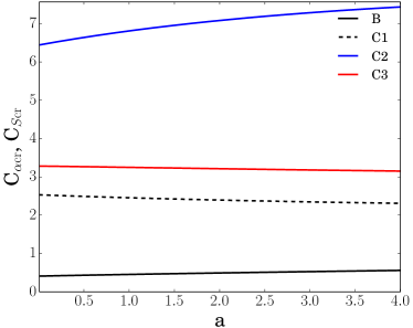
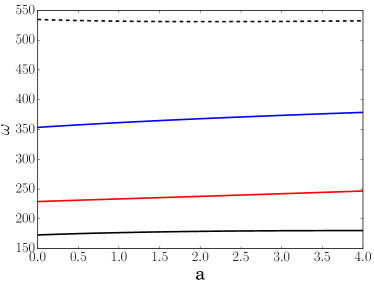
Figure 1: Panel a) shows the dynamo instability threeshold for different models. For the model B it shows the critical parameter $C_{\alpha}$ and for the model C1 and C2 it shows critical parameter $C_{S}$ ; b) shows the frequency of the first unstable dipole- and quadrupole-like modes;

In this section we examine the effect of the anisotropic mixing using the benchmark model presented by Jouve et al. (2008)(hereafter J08). In this case we use the simplest representation for the mean electromotive force with the isotropic $\alpha$-effect, $\boldsymbol{\boldsymbol{\mathcal{E}}}=\alpha\overline{\mathbf{B}}+\boldsymbol{\boldsymbol{\mathcal{E}}}^{(dif)}$, where $\boldsymbol{\boldsymbol{\mathcal{E}}}^{(dif)}$ is given by Eq.(3). Thus, we have the following dynamo equations:

$$\frac{\partial A}{\partial T} = \tilde{\eta}\frac{\partial^{2}A}{\partial x^{2}}+\tilde{\eta}\left(1+\frac{a}{2}\right)\frac{\sin\theta}{x^{2}}\frac{\partial}{\partial\theta}\frac{1}{\sin\theta}\frac{\partial A}{\partial\theta}$$

$$+ \frac{\tilde{\eta}a}{2x}\frac{\partial A}{\partial x}-R_{e}\left(\frac{\tilde{U}_{\theta}}{x}\frac{\partial A}{\partial\theta}+\tilde{U}_{r}\frac{\partial A}{\partial x}\right)$$

$$+ C_{\alpha}\tilde{\alpha}_{0}x\cos\theta\sin^{3}\theta B+C_{S}\tilde{S}_{0}x\cos\theta\sin\theta B\left(0.7R_{\odot},\theta,T\right)$$

$$\frac{\partial B}{\partial T} = \frac{C_{\Omega}}{x}\left(\frac{\partial\tilde{\Omega}}{\partial x}\frac{\partial A}{\partial\theta}-\frac{\partial\tilde{\Omega}}{\partial\theta}\frac{\partial A}{\partial x}\right)+\frac{a}{2x}\frac{\partial}{\partial x}\left(\tilde{\eta}B\right)$$

$$+ \left(1+\frac{a}{2}\right)\frac{\tilde{\eta}}{x^{2}}\frac{\partial}{\partial\theta}\frac{1}{\sin\theta}\frac{\partial\sin\theta B}{\partial\theta}+\frac{1}{x}\frac{\partial}{\partial x}\tilde{\eta}\frac{\partial xB}{\partial x}$$

$$- \frac{R_{e}}{x}\left(\frac{\partial\left(x\tilde{U}_{r}B\right)}{\partial x}+\frac{\partial\tilde{U}_{\theta}B}{\partial\theta}\right),$$

where $C_{\alpha}={\displaystyle\frac{\alpha_{0}R^{3}}{\eta_{0}}}$, $C_{\Omega}={\displaystyle\frac{\Omega_{0}R^{2}}{\eta_{0}}}$, $R_{e}={\displaystyle\frac{U_{0}R}{\eta_{0}}}$, and $C_{S}$ is to control the amplitude of the Babcock-Leighton effect, $x=r/R_{\odot}$, and $T=t{\displaystyle\frac{\eta_{0}}{R_{\odot}^{2}}}$, where $\eta_{0}=10^{11}\textnormal{cm}^{2}\textnormal{s}^{-1}$ is the background level of the magnetic turbulent diffusivity. The radial profiles of the angular velocity, $\tilde{\Omega}$, the turbulent diffusivity, $\tilde{\eta}$, the $\alpha$-effect, $\tilde{\alpha}_{0}$, and the Babcock-Leighton effect, $\tilde{S}_{0}$ , are shown in Figure2.1(a,b). They are the same as in (Jouve et al., 2008)( J08). The dynamo domain of benchmark model is located between $r_{b}=0.65R_{\odot}$ and $r_{e}=R_{\odot}$.

The meridional flow is modeled in the form of stationary circulation cells stacking cells along the radius. The pattern is modeled by the stream functions $\Psi$:

$$\Psi = -\frac{2}{\pi}\frac{\left(x-x_{b}\right)^{2}}{1-x_{b}}\sin\left(\frac{\pi\left(x-x_{b}\right)}{\left(1-x_{b}\right)}\right)\sin\theta\cos\theta$$ (5)

$$\Psi = \frac{2c_{0}}{\pi\left((1+\exp(-200(x-x_{0})\right)}\left(\frac{1-x}{x}\right)^{1.5}\left(\frac{\partial P_{2}}{\partial\theta}+m\frac{\partial P_{4}}{\partial\theta}\right)\times\sum_{n=1}^{3}c_{n}\sin\left(\frac{n\pi\left(x-x_{b}\right)}{\left(1-x_{b}\right)}\right)$$ (6)

where, $P_{2,4}$ are the Legendre polynomials, $x_{b}=r_{b}/R$ is the inner boundary of the integration domain; parameter $m$ controls the number of cells in latitude; $c_{0}$ is the constant to normalize the maximum of the flow amplitude to 1; $c_{1}$, $c_{2}$ and $c_{3}$control the amplitudes of flows in the stacking cells. The velocity field of the flow is given by $\overline{\mathbf{U}}^{p}={\displaystyle U_{0}\boldsymbol{\nabla}\times}\left(\mathbf{e_{\phi}\Psi}\right)$, in the case of one cell circulation (model C1, Eq.5) and $\overline{\mathbf{U}}^{p}={\displaystyle\frac{U_{0}}{\overline{\rho}}\boldsymbol{\nabla}\times}\left(\mathbf{e_{\phi}\Psi}\right)$ for the models C2 and C3, (the case Eq.6). The $U_{0}$ is a characteristic flow speed. In the cases C2 and C3 we choose $x_{0}=0.71$ to cut off penetration of circulation below $r=0.7R_{\odot}$. The stream function is similar to the one of (Pipin & Kosovichev, 2013) with a modification to control the penetration of the meridional circulation below the convection zone. The circulation pattern is illustrated in Figure 2.1. We will use the same value for the $\Omega$-effect, as in the J08, $C_{\Omega}=1.4\times 10^{5}$. The parameters of the benchmark models are listed in the Table1.

Summarizing, we conclude that models B and C1 correspond to those studied by J08. Models C2 and C3 are given for comparison. The case C2 is motivated by recent results of helioseismology results (Zhao et al., 2013). The radial profile of the latitudinal component of meridional circulation (see, Fig.2.1(c, blue curve)) and geometry of the flow Fig.2.1(e)) are close to results detected by helioseismology inversion. Numerical simultaions often produce the multi-cellular meridional circulation which can have three cells stacked along the radial direction (Käpylä et al., 2012; Guerrero et al., 2013). This question is addressed for the models with triple-cell circulation pattern (Fig.2.1(c, red curve) and Fig.2.1(f)). In this case our circulation pattern is only qualitatively reproduce the numerical simulations. The study of this case help us to highlight the important difference between the models for the case of the odd and even number of circulation cells stacked along the radius.

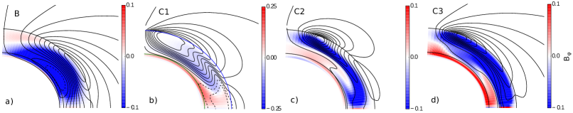
Figure 2: Panel a) shows a snapshot of the large-scale magnetic field inside the convection zone for the benchmark dynamo model B with $a=4$. The field lines show of the poloidal component of the mean magnetic field, and the toroidal magnetic field is shown by the background images. Panel b) shows the same for the model C1; c) shows the same as b) for the model with the double-cell meridional circulation, the model C2; d) shows the same for the model C3 and $a=4$.

2.2 Results for benchmark models

Here, we show results of the eigen-value problem solution for the benchmark models listed in the Table 1. The dynamo instability develops, when a non-dimensional parameters, $C_{\alpha}$, which controls the magnitude of the $\alpha$-effect, or, $C_{S}$, which controls the strength of the Coriolis force acting on the flux-tube rising through the solar convection zonet, exceeds the critical value. Figure 1(a) shows the critical threshold parameters $C_{\alpha cr}$ and $C_{Scr}$ for the dynamo instability of the dipole like modes as a function of the anisotropy parameter, $a$. Figure 1(b) shows the frequency of the first unstable mode. The cases B and C1 correspond to those studied by Jouve et al. (2008)(J08). In these cases we have $C_{\alpha cr}=0.408$, $\omega=173$ and $C_{Scr}=2.53$ $\omega=534$ for $a=0$. This is in perfect agreement with J08. The main result is that the critical threshold dynamo parameters, as well as, the frequency (and period) of the dynamo oscillations vary rather little with variation of $a$. Moreover, in the cases B and C2 (even number of circulation cells), the dynamo threshold is slowly growing with increasing of $a$. On the other hand, the cases C1 and C3 show the slowly decreasing dynamo threshold with increasing of $a$. As we have guessed previously, (Pipin & Kosovichev, 2013), there is a similarity for the dynamo regimes operating with even or odd number of the circulation cells stacking along the radius. Another interesting finding is that the dynamo period is growing with the increasing number of circulation cells (see also Hazra et al. 2013). This is not directly related to the effect of the anisotropy of turbulent diffusion.

Figures 1(a,b) show the threshold parameters for the first unstable dipole-type eigen modes. The threshold parameters of the quadrupole type modes vary in similar way. For the model B, the first unstable dipole type mode has smaller $C_{\alpha cr}$ than the first unstable quadrupole type mode for $a<2$. Both modes have close frequencies. For the model C1 the first unstable dipole type mode is preferable for the all range of $a$. Meanwhile the frequency of the first unstable quadrupole type mode is as twice smaller than the frequency of the first unstable dipole type mode. In the model C2 the first unstable mode has the quadrupole type symmetry for the all range of $a$. The opposite is true for the model C3. The results for the parity preference are listed in the Table 1.

The typical snapshots of the magnetic field distributions for the models B,C1,C2 and C3 for the case of $a=4$ are illustrated in Figure 2. The time-latitude diagrams of the toroidal magnetic field at $r=0.7R_{\odot}$and the radial magetic field at the surface are shown in Figure 3. The model C1 and C3 have some qualitative agreement with observations. However, the butterfly wings of the toroidal magnetic field are to wide in compare with observations. Also, for the large anisotropy paprameter $a=4$ the model C1 has the wrong phase relation between the maxims of toroidal magnetic field in equatorial region and inversion of the radial magnetic field at the pole. The model C3 reproduces the phase relation in a better way, though the inversion of the polar field occurs about 5 years in advance to the maximum of the toroidal field in equatorial region. We have to note that for the case of $a=0$ the model C3 shows much longer polar branch of the radial magnetic field. Thus, the including the anisotropy of the turbulent diffusion in the model brings this model in the better agreement with observations. In the models B and C2 the toroidal field drifts to the pole at the bottom of the convection zone. In the model C2, the meridional circulation moves the toroidal field toward equator in the middle of the convection zone. Similar to the models C1 and C3, in the models B and C2 the anisotropy of turbulent diffusivity decrease the polar branch of the radial magnetic field evolution. Additionally, in the model B the poleward drifting dynamo wave of the toroidal magnetic field converge to the steady wave near the surface.

Summarizing consideration of the benchmark models we conclude, that the radial anisotropy of the turbulent diffusivity does not significantly change the conditions for the dynamo instability. It does not impact very much the dynamo period as well. However, we find that it can result to the shorter polar branch of the radial magnetic field at the surface. For the models B, C2 and C3, in the upper part the convection zone the poleward migration of the toroidal magnetic field dominates. This migration is reversed in the dynamo model with the subsurface shear of the angular velocity, which we study in the next section.

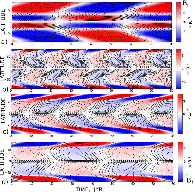
Figure 3: Panel a) shows the time-latitude evolution of the toroidal magnetic field at the bottom of the convection zone (contours) and the radial magnetic field (background image) for the benchmark dynamo model B for the anisotropy parameter $a=4$; b) shows the same as (a) for the model C1; c) shows the same for the model C2; d) shows the same for the model C3.

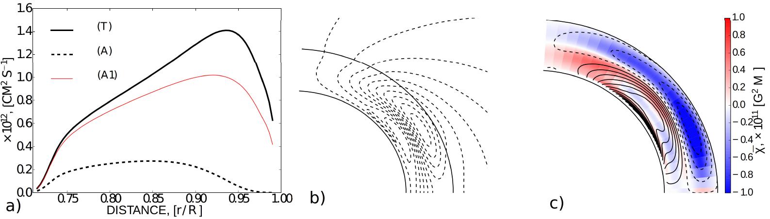
Figure 4: Panel a) Turbulent diffusion coefficients as a function of radius: $\eta^{(A)}$ is the anisotropic part due to rotation, $\eta^{(A1)}$is anisotropic diffusivity for $a=3$, $\eta^{(T)}$is the total diffusivity. Panel b) snapshot of the poloidal magnetic field lines; c) shows contours for the toroidal magnetic field (contours $\pm 1$kG) and the small-scale magnetic helicity is in the background.

2.3 Solar dynamo model with subsurface shear

In this section we consider the anisotropy effects in the model, which we developed in our recent papers (Pipin & Kosovichev, 2011a, 2013; Pipin et al., 2012). The mean electromotive force is given as follows (Pipin 2008, hereafter, P08).

$$\mathcal{E}_{i}=\left(\alpha_{ij}+\gamma_{ij}^{(\Lambda)}\right)\overline{B}_{j}-\left(\eta_{ijk}+\eta_{ijk}^{(\delta)}\right)\nabla_{j}\overline{B}_{k}+\mathcal{E}_{i}^{(A)}.$$ (7)

where $\mathcal{E}_{i}^{(A)}$ is the anisotropic part of magnetic diffusivity for the prescribed anisotropy of the backgroud turbulence model. It is given by Eqs (4) and (A20). The tensor $\alpha_{ij}$ describes the $\alpha$-effect. It includes hydrodynamic ($\alpha_{ij}^{(H)}$) and magnetic ($\alpha_{ij}^{(M)}$) helicity contributions:

$$\alpha_{ij} = C_{\alpha}\psi_{\alpha}\sin^{2}\theta\alpha_{ij}^{(H)}+\alpha_{ij}^{(M)}$$ (8)

The $\alpha$-quenching function $\psi_{\alpha}=-3/4\phi_{6}^{(a)}\left(\beta\right)$ depends on $\beta={\displaystyle\left|\overline{B}\right|/\sqrt{\mu_{0}\overline{\rho}\overline{u^{2}}}}$, and $\phi_{6}^{(a)}$ is given in P08. The magnetic helicity contribution to the $\alpha$-effect is defined as follows (P08):

$$\alpha_{ij}^{(M)}=2\left(f_{2}^{(a)}\delta_{ij}-f_{1}^{(a)}\frac{\Omega_{i}\Omega_{j}}{\Omega^{2}}\right)\frac{\overline{\chi}\tau_{c}}{\mu_{0}\overline{\rho}\ell^{2}}$$ (9)

The functions $f_{1,2}^{(a)}$ describe the effect of rotation and can be found in P08. The evolution of magnetic helicity $\overline{\chi}=\overline{\mathbf{a}\cdot\mathbf{b}}$, where $\mathbf{a}$ is the fluctuating vector-potential, $\mathbf{b}$- the fluctuating magnetic field is determined from the conservation law (see, Pipin, 2013; Pipin et al., 2013):

$$\frac{\partial\overline{\chi}^{(tot)}}{\partial t}=-\frac{\overline{\chi}}{R_{m}\tau_{c}}-\eta\overline{\mathbf{B}}\cdot\mathbf{\overline{J}}-\mathbf{\left(\overline{U}\cdot\boldsymbol{\nabla}\right)}\overline{\chi}^{(tot)}$$ (10)

where $\overline{\chi}^{(tot)}=\mathbf{\overline{A}}\cdot\overline{\mathbf{B}}+\overline{\chi}$ is the total magnetic helicity. In the model we assume $R_{m}=10^{6}$.

The turbulent pumping coefficient in Eq(7), $\gamma_{ij}^{(\Lambda)}$, depends on the mean density and turbulent diffusivity stratification, and also on the Coriolis number $\Omega^{*}=2\tau_{c}\Omega_{0}$, where $\tau_{c}$ is a typical convective turnover time, and $\Omega_{0}$ is the angular velocity. For detailed expressions of $\gamma_{ij}^{(\Lambda)}$ see the above cited papers. The turbulent diffusivity is anisotropic due to the Coriolis force, and is given by:

$$\eta_{ijk}=3\eta_{T}\left\{\left(2f_{1}^{(a)}-f_{2}^{(d)}\right)\varepsilon_{ijk}-2f_{1}^{(a)}\frac{\Omega_{i}\Omega_{n}}{\Omega^{2}}\varepsilon_{njk}\right\}.$$ (11)

We also include the nonlinear effects of magnetic field generation induced by the large-scale current and global rotation, which are usually called the $\Omega\times J$-effect or the $\delta$ dynamo effect (Rädler, 1969). Their importance is supported by the numerical simulations (Käpylä et al., 2008; Schrinner, 2011). We use the equation for $\eta_{ijk}^{(\delta)}$ which was suggested in P08 (also, see, Rogachevskii & Kleeorin, 2004):

$$\eta_{ijk}^{(\delta)}=3\eta_{T}C_{\delta}f_{4}^{(d)}\frac{\Omega_{j}}{\Omega}\left\{\tilde{\varphi}_{7}^{(w)}\delta_{ik}+\tilde{\varphi}_{2}^{(w)}\frac{\overline{B}_{i}\overline{B}_{k}}{\overline{B}^{2}}\right\},$$ (12)

where, $C_{\delta}$ measures the strength of the $\Omega\times J$ effect, $\tilde{\varphi}_{2,7}^{(w)}\left(\beta\right)$ are normalized versions of the magnetic quenching functions $\varphi_{2,7}^{(w)}$ given in P08. They are defined as follows, $\tilde{\varphi}_{2,7}^{(w)}\left(\beta\right)=\frac{5}{3}\varphi_{2,7}^{(w)}\left(\beta\right)$. The functions $f_{\{1,2\}}^{(a,d)}$in Eqs (8,11, 12) depend on the Coriolis number. They can be found in P08, as well.

Following Pipin & Kosovichev (2011b) we use a combination of the “open” and “closed” boundary conditions at the top, controlled by a parameter $\delta=0.99$:

$$\delta\frac{\eta_{T}}{r_{e}}B+\left(1-\delta\right)\mathcal{E}_{\theta}=0.$$ (13)

This is similar to the boundary condition discussed by Kitchatinov et al. (2000). This condition results to penetration of the toroidal field to the surface, which increase the efficiency of the subsurface shear layer (Pipin & Kosovichev, 2011b). For the poloidal field we apply a condition of smooth transition from the internal poloidal field to the external potential (vacuum) field.

Summing up, the model includes magnetic field generation generation effects due to the differential rotation ($\Omega$ -effect), turbulent kinetic helicity (the anisotropic $\alpha$-effect) and interaction of large-scale currents with the global rotation, usually called $\Omega\times J$-effect or $\delta$-effect (Rädler, 1969; Käpylä et al., 2008; Schrinner, 2011). For the differential rotation, we use an analytical fit to the recent helioseismology results of Howe et al. (2011) (see, Fig.1(c) in Pipin & Kosovichev, 2013). The subsurface rotational shear layer provides additional energy for the toroidal magnetic field generation, and also induces the equator-ward drift of the toroidal magnetic field (Pipin & Kosovichev, 2011b). We also take into account the turbulent transport due to the mean density and turbulent intensity gradients (so-called “gradient pumping”). The model includes also the magnetic helicity balance, as described by Pipin et al. (2013) . The contribution of the anisotropic diffusion to the mean electromotive force is given by Eqs(A20).

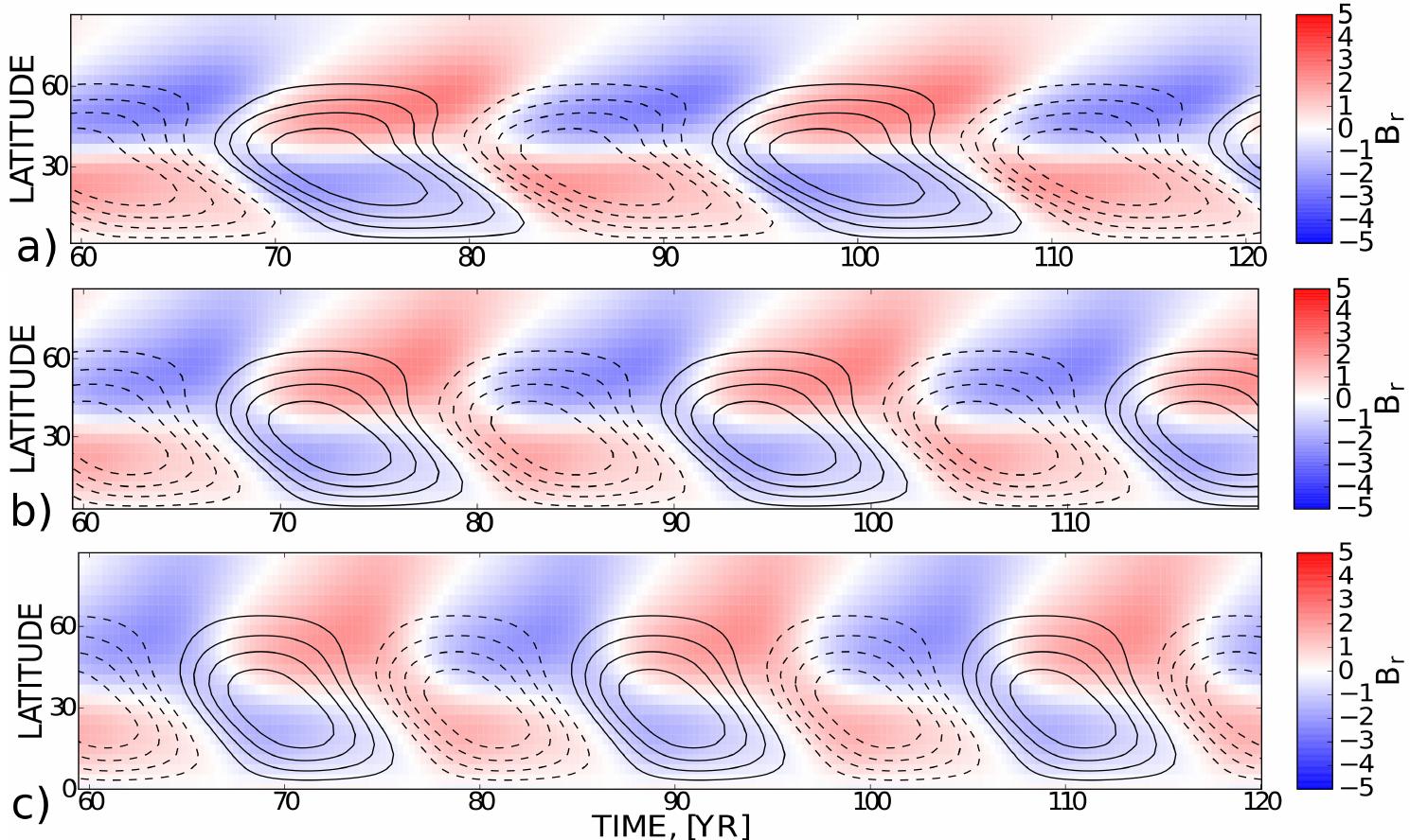
Figure 5: (a) the time - latitude variations (“butterfly diagrams”) for the model with $a=0$; (b) the same for the $a=2$ (c) the same for the $a=4$ . The toroidal field near the surface, at $r=0.92R_{\odot}$, is shown by contours (plotted for $\pm 100$G range), and the surface radial magnetic field is shown by background red-blue images.

The turbulent diffusivity profiles for $a=3$ are shown in Figure 4(a). We see that with the anisotropy effect the total effective diffusivity is greater than $10^{12}$ cm²/s in the upper part of the convection zone. This is close to the turbulent magnetic diffusivity estimated from the sunspot decay rate (Martinez Pillet et al., 1993) and also from the cross-helicity observations (Rüdiger et al., 2011; Pipin et al., 2011).

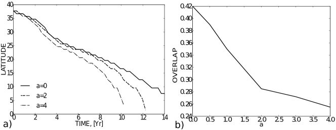
Figure 6: Panel a) The latitudinal location of maxima of the toroidal magnetic field flux in the subsurface shear layer for the model with $a=0,2,4$; b) the overlap time (relative to the cycle length) between the subsequent cycles as a function of the anisotropy parameter $a$.

Typical snapshots for the magnetic field and magnetic helicity distributions in the solar convection zone are shown in Figure 4(b,c). Similar to the benchmark models we see that the toroidal magnetic field is concentrated to the boundaries of the convection zone. The near surface magnetic field is weaker than the bottom field during most of the dynamo cycle.

Figure 5 shows the time -latitude diagram of the toroidal magnetic field in the subsurface shear layer $r=0.92R_{\odot}$ and for the radial magnetic field at the top of the domain $r=0.99R_{\odot}$. Their behavior is similar to the solar cycles. We see that the cycle period decreases from 14 Yrs to 10 Yrs when $a$ increases from $0$ to 4. For $a=4$ the model has the total effective magnetic diffusivity greater than $10^{12}$ cm²/s in a large part of the convection zone. Still, the dynamo model reproduces correctly the solar cycle period and the patterns of the toroidal and poloidal magnetic field evolution.

Another interesting feature which is demonstrated by Figure 5 is that the overlap between the cycles decreases when we increase the anisotropy parameter $a$. We investigated this feature in details for the distributed dynamo model without meridional circulation. To quantify the overlap between the subsequent cycles we examine the latitudinal drift of the toroidal flux maxima in the subsurface shear layer at $r=0.92R_{\odot}$(see Figure 6a). We restrict our consideration to the latitudinal range $0-40^{\circ}$, and compute the relative overlap between the curves that belong to subsequent cycles. Figure 6b shows the results for the models with $0\leq a\leq 4$. The relative overlap time between the subsequent cycles decreases from $0.42$(5 Yrs) to $0.25$(2.5 Yrs) when $a$ spans from $0$ to $4$. The speed of the dynamo wave latitudinal migration remains almost the same for all $a$. This means that the dynamo wave is not transformed from the running to steady type with the increase of $a$.

3 Discussion and conclusion

In this paper we have examined influence of anisotropic turbulence in the solar convection zone on magnetic diffusivity and properties of mean-field dynamo models, including the simplified benchmark model (Jouve et al., 2008) and the distributed-dynamo model with the subsurface shear layer and a detailed formulation of the mean-electromotive force (Pipin & Kosovichev, 2011a; Pipin et al., 2013; Pipin & Kosovichev, 2013). To characterized the anisotropy, we, similar to Rüdiger et al. (2005), use parameter $a$ derived as a relative difference between horizontal and vertical turbulent RMS velocities.

The strength of the anisotropy parameter depends on the theoretical models of turbulent flows. In the simple case of the mixing length theory, it is restricted to the range $a=0-4$ ($a=0$ corresponds to isotropic flows). The nonlocal stellar convection theory (Deng et al., 2006) suggests $a\sim 3.5$. Numerical simulations of the solar convection showed evidence for a stronger anisotropy, which may reach $a\sim 10$ (e.g., Miesch et al. 2008; Guerrero et al. 2013). This anisotropy results from the global rotation effect on convective motions, and forms the “banana”-like giant convection cells in the meridional direction. It is important to note that in the simulations such anisotropic convection becomes visible even in the subsurface shear layer below $0.95R_{\odot}$ where the analytical mixing-length estimations of the mean-field diffusivity coefficients show a small anisotropy. However, the current simulations still do not accurately reproduce the convection zone dynamics. Therefore, we considered the anisotropic parameter $a$ as a free parameter. The analytical calculations presented in Appendix showed that the effect of turbulent mixing in the horizontal direction is quenched by rotation while the effective structure of the given anisotropic difusivity tensor remains the same as in the case of slow rotation.

Study the benchmark models suggests that the dynamo threshold parameters of the models change only a little with increase of the anisotropy parameter $a$. This could be expected from analysis given by Kitchatinov (2002). The interesting new finding is that the dynamo threshold can decrease with the increase of $a$. This is found for the models with the odd number of circulation cell stacked along the radius. For the case of the zero and double-cell circulation we find the opposite behaviour.

In the benchmark models the equatorial drift of the toroidal magnetic field depends on the amplitude and the type of meridional circulation. The model B, which has no meridional circulation, does not have equatorial branch of the toroidal magnetic field in the convection zone. This is also due to the absence of the subsurface shear layer. The detailed solar dynamo model, which was discussed in the subsection 2.3, has the equatorial migration of the toroidal magnetic field in the upper part of the convection zone. This effect is induced by the subsurface shear layer. The effect of the subsurface shear on the large-scale dynamo was suggested earlier by Brandenburg (2005). We note the particular role of the boundary condition (Eq.13) for the subsurface shear to be feasible for the large-scale dynamo. This condition results to penetration of the toroidal field to the surface, which increase the efficiency of the subsurface shear layer (Pipin & Kosovichev, 2011b). Thus, the model can produce the equatorial drift of the toroidal field in the upper part of the convection zone (above 0.9$R_{\odot}$) for rather small equatorial turbulent pumping, which operates in the bulk of the convection zone with amplitude less than 1 m/s (see, Pipin & Kosovichev, 2011a). This is different to the model sugested by Käpylä et al. (2006), who employed, in addition to subsurface shear, the strong turbulent pumping effects in the bulk of the convection zone. The reader can look for the detailed discussion effect of subsurface shear layer in above cited papers.

In the flux transport models C2 and C3 the equatorial branch of the toroidal field is induced by the equatorial parts of the meridional circulation cells. Thus, the model C2 has equatorial migration of the toroidal magnetic field in the middle of the convection zone (see more details in Pipin & Kosovichev 2013). The model C3, with the triple-cell circulation has in addition the equatorial migration near the bottom of the convection zone. The physical interpretation of these types of models suggests that poloidal field at the surface is produced directly from the buoyant flux tubes that come from the bottom of the convection zone. In this case the model with double-cell circulation is not solar-like. The model with the triple-cell circulation has a qualitatve agreement with observations, though the polar reversal of the radial magnetic field, $\overline{B}_{r}$, occurs about 5 years ahead of the maximum of the toroidal magnetic field, $\overline{B}_{\phi}$, in equatorial region. This model has the dynamo period as twice as large compare to the solar cycle in the case $a=4$. For the case $a=0$ model C3 has the larger dynamo period about 30 Yrs, though the phase relation between activity of $\overline{B}_{r}$ and $\overline{B}_{\phi}$ is in a better agreement with observations.

We made addtional calculations for the distributed solar dynamo models like that discussed in subsection 2.3 including the effect of multi-cells circulation. For the case of the double-cell circulation we reproduced our results from the previous paper (see, Pipin & Kosovichev, 2013). We confirm the effect of the decreasing overlap between the subsequent cycles with the increasing parameter of the anisotropy $a$. The case of the triple-cell circulation is found to be similar to the model C3. However in this case the correct phase relation between activity of $\overline{B}_{r}$ and $\overline{B}_{\phi}$ holds only for the upper part of the convection zone, where similar to the model with double cell circulation we have the equatorial drift of the toroidal magnetic field because of equatorward flow of the meridional circulation. The results of that model are similar to results of the numerical simulation reported by Käpylä et al. (2012). Note, that differential rotation profile in their paper is different from the solar case.

With the effects of anisotropy the total magnetic diffusivity reaches values of about $10^{12}$cm²/s in the layer $0.85-0.95R_{\odot}$, which are consistent with estimates from the sunspot decay rate (Martinez Pillet et al., 1993) and the cross-helicity observations (Rüdiger et al., 2011). We found that the anisotropy affects the overlap time between the subsequent cycles. When the anisotropy is larger, the overlap is smaller. This effect is related to stronger concentration of the toroidal magnetic field near the bottom boundary of the convection zone due to anisotropy, and also as a consequence of a faster migration of the dynamo wave in the subsurface shear layer. In general, our model is consistent with the paradigm of solar dynamo operating in the bulk of the convection zone and “shaped” in the subsurface roatational shear layer.

4 Appendix A

To compute the electromotive force $\mathcal{E}$ for the anisotropic MHD turbulence we write equations (1) and (2) in the Fourier space:

$$\left(\frac{\partial}{\partial t}+\eta z^{\prime 2}\right)\hat{b}_{j} \!=\! iz^{\prime}_{l}\int\left\{\widehat{u}_{j}(\mathbf{z^{\prime}-q)}B_{l}\left(\mathbf{q}\right)-\widehat{u}_{l}\left(\mathbf{z^{\prime}-q)}B_{j}\left(\mathbf{q}\right)\right.\right\}\mathrm{d}\mathbf{q}+\widehat{\mathbf{\mathfrak{G}}}_{j}.$$ (A1)

$$\left(\frac{\partial}{\partial t}+\nu z^{2}\right)\hat{u}_{i} \!=\! \!\hat{f}_{i}+\hat{\mathfrak{F}}_{i}-2(\Omega\hat{z})(\hat{z}\times\hat{u})_{i}+\frac{i\pi_{if}}{\mu}z_{l}\int\{\widehat{b}_{l}(\mathbf{z-q)}B_{f}(\mathbf{q})+\widehat{b}_{f}(\mathbf{z-q)}B_{l}(q)\}\mathrm{d}\mathbf{q},$$ (A2)

where the turbulent pressure was excluded from (Eq.2) by convolution with tensor $\pi_{ij}(\mathbf{z)}=\delta_{ij}-\hat{z}_{i}\hat{z}_{j}$, where $\delta_{ij}$ is the Kronecker symbol, and $\widehat{\mathbf{z}}$ is a unit wave vector. The equations for the second-order moments that make contributions to the mean electromotive force can be found directly from Eqs.(A1, A2). We consider the high Reynolds number limit and discard the microscopic diffusion terms. Using the $\tau$-approximation, in which the third order products of the fluctuating fields are approximated by the corresponding relaxation terms of the second-order contributions (see, Rädler et al., 2003; Rogachevskii & Kleeorin, 2003; Brandenburg & Subramanian, 2005; Pipin, 2008; Rogachevskii et al., 2011), we arrive to

$$\frac{\hat{\varkappa}_{ij}(\mathbf{z},\mathbf{z}^{\prime})}{\tau^{*}\left(z\right)}+2(\Omega\hat{z})\varepsilon_{inm}\hat{z}_{n}\hat{\varkappa}_{mj}(\mathbf{z},\mathbf{z}^{\prime}) = iz^{\prime}_{l}\int\left\{\hat{v}_{ij}(\mathbf{z},\mathbf{z}^{\prime}-\mathbf{q})\overline{B}_{l}(\mathbf{q})-\hat{v}_{il}(\mathbf{z},\mathbf{z}^{\prime}-\mathbf{q})\overline{B}_{j}(\mathbf{q})\right\}\mathrm{d}\mathbf{q}$$

$$+ \frac{i}{\mu}z_{l}\pi_{if}\int\hat{m}_{lj}(\mathbf{z}-\mathbf{q},\mathbf{z}^{\prime})\overline{B}_{f}(\mathbf{q})\mathrm{d}\mathbf{q}$$

$$+ \frac{i}{\mu}z_{l}\pi_{if}\int\hat{m}_{fj}(\mathbf{z}-\mathbf{q},\mathbf{z}^{\prime})\overline{B}_{l}(\mathbf{q})\mathrm{d}\mathbf{q},$$

$$\frac{\hat{v}_{ij}(\mathbf{z},\mathbf{z}^{\prime})}{\tau^{*}\left(z\right)} = \frac{v_{ij}^{(0)}}{\tau^{*}\left(z\right)}-2(\Omega\hat{z})\varepsilon_{inm}\hat{z}_{n}\hat{v}_{mj}(\mathbf{z},\mathbf{z}^{\prime})-2(\Omega\hat{z}^{\prime})\varepsilon_{jnm}\widehat{z^{\prime}}_{n}\hat{v}_{im}(\mathbf{z},\mathbf{z}^{\prime})$$

$$+ \frac{i\pi_{if}}{\mu}z_{l}\int\{\hat{\varkappa}_{lj}(\mathbf{z}^{\prime},\mathbf{z}-\mathbf{q})\overline{B}_{f}(\mathbf{q})+\hat{\varkappa}_{fj}(\mathbf{z}^{\prime},\mathbf{z}-\mathbf{q})\overline{B}_{l}(q)\}\mathrm{d}\mathbf{q}$$

$$+ \frac{i\pi_{jf}}{\mu}z^{\prime}_{l}\int\{\hat{\varkappa}_{il}(\mathbf{z},\mathbf{z}^{\prime}-\mathbf{q})\overline{B}_{f}(\mathbf{q})+\hat{\varkappa}_{if}(\mathbf{z},\mathbf{z}^{\prime}-\mathbf{q})\overline{B}_{l}(q)]\mathrm{d}\mathbf{q},$$

$$\frac{\hat{m}_{ij}(\mathbf{z},\mathbf{z}^{\prime})}{\tau^{*}\left(z\right)} = iz^{\prime}_{l}\int\{\hat{\varkappa}_{jl}(\mathbf{z}^{\prime}-\mathbf{q},\mathbf{z})\left.\overline{B}_{l}(\mathbf{q})-\hat{\varkappa}_{li}(\mathbf{z}^{\prime}-\mathbf{q},\mathbf{z})\overline{B}_{j}(\mathbf{q})\right\}\mathrm{d}\mathbf{q}$$

$$+ iz_{l}\int\{\hat{\varkappa}_{ij}(\mathbf{z}-\mathbf{q},\mathbf{z}^{\prime})\left.\overline{B}_{l}(\mathbf{q})-\hat{\varkappa}_{lj}(\mathbf{z}-\mathbf{q},\mathbf{z}^{\prime})\overline{B}_{i}(\mathbf{q})\right\}\mathrm{d}\mathbf{q}$$

$$+ \frac{m_{ij}^{(0)}(\mathbf{z},\mathbf{z}^{\prime})}{\tau^{*}\left(z\right)},$$

where we introduced the ensemble averages $\hat{v}_{ij}(\mathbf{z},\mathbf{z}^{\prime})=\overline{\mathbf{u}_{i}\left(\mathbf{z}\right)\mathbf{u}_{j}\left(\mathbf{z}^{\prime}\right)}$, $\hat{\varkappa}_{ij}(\mathbf{z},\mathbf{z}^{\prime})=\overline{\mathbf{u}_{i}\left(\mathbf{z}\right)\mathbf{b}_{j}\left(\mathbf{z}^{\prime}\right)}$, $\hat{m}_{ij}(\mathbf{z},\mathbf{z}^{\prime})=\overline{\mathbf{b}_{i}\left(\mathbf{z}\right)\mathbf{b}_{j}\left(\mathbf{z}^{\prime}\right)}$; the superscript ⁽⁰⁾ stands for the background state (when the mean-field is absent) of these correlations. The reader can find a comprehensive discussion of the $\tau$ -approximation in the above cited papers. Furthermore, the contributions of the mean magnetic field in the equation for the turbulent stresses, $\hat{v}_{ij}$, will be neglected because they give nonlinear terms in the cross-helicity tensor, $\hat{\varkappa}_{ij}$.

Next, we solve Eqs(4,4,4) in a linear approximation for the mean field $\overline{\mathbf{B}}$, also neglecting effects of background magnetic fluctuations in the further analysis. Thus, we obtain

$$\hat{\varkappa}_{ij}(\mathbf{z},\mathbf{z}^{\prime}) = i\tau^{*}\left(z\right)z^{\prime}_{l}D_{ip}(\mathbf{z})\int\left\{\hat{v}_{pj}(\mathbf{z},\mathbf{z}^{\prime}-\mathbf{q})\overline{B}_{l}(\mathbf{q})-\hat{v}_{pl}(\mathbf{z},\mathbf{z}^{\prime}-\mathbf{q})\overline{B}_{j}(\mathbf{q})\right\}\mathrm{d}\mathbf{q}$$

$$+ D_{ip}(\mathbf{z})\frac{iz_{l}\tau^{*}\left(z\right)}{\mu}\pi_{pf}\int\hat{m}_{lj}(\mathbf{z}-\mathbf{q},\mathbf{z}^{\prime})\overline{B}_{f}(\mathbf{q})\mathrm{d}\mathbf{q}$$

$$+ D_{ip}(\mathbf{z})\frac{iz_{l}\tau^{*}\left(z\right)}{\mu}\pi_{pf}\int\hat{m}_{fj}(\mathbf{z}-\mathbf{q},\mathbf{z}^{\prime})\overline{B}_{l}(\mathbf{q})\mathrm{d}\mathbf{q},$$

$$\hat{v}_{ij} = \mathcal{D}_{injm}(\mathbf{z},\mathbf{z}^{\prime})v_{nm}^{(0)}$$

$$+ \mathcal{D}_{injm}(\mathbf{z},\mathbf{z}^{\prime})\frac{i\tau^{*}\left(z\right)\pi_{nf}}{\mu}z_{l}\int\{\hat{\varkappa}_{lm}(\mathbf{z}^{\prime},\mathbf{z}-\mathbf{q})\overline{B}_{f}(\mathbf{q})+\hat{\varkappa}_{fm}(\mathbf{z}^{\prime},\mathbf{z}-\mathbf{q})\overline{B}_{l}(q)\}\mathrm{d}\mathbf{q}$$

$$+ \mathcal{D}_{injm}(\mathbf{z},\mathbf{z}^{\prime})\frac{i\tau^{*}\left(z\right)\pi_{mf}}{\mu}z^{\prime}_{l}\int\{\hat{\varkappa}_{nl}(\mathbf{z},\mathbf{z}^{\prime}-\mathbf{q})\overline{B}_{f}(\mathbf{q})+\hat{\varkappa}_{if}(\mathbf{z},\mathbf{z}^{\prime}-\mathbf{q})\overline{B}_{l}(q)]\mathrm{d}\mathbf{q},$$

where,

$$D_{ip}(z) = \frac{\delta_{ip}+E_{ip}}{1+\psi_{\Omega}^{2}},$$

$$\mathcal{D}_{injm}(\mathbf{z},\mathbf{z}^{\prime}) = \left\{\frac{\delta_{if}\hat{N}+2E_{if}}{\hat{N}^{2}+4\psi_{\Omega}^{2}}\right\}(\delta_{jm}(\delta_{fn}+E_{fn})-\delta_{fn}\tilde{E}{}_{jm})$$

$$E_{nk} = \frac{2(\Omega\cdot\mathbf{z})\tau}{\mathbf{z}^{2}}z_{p}\varepsilon_{nkp},\,\tilde{E}{}_{ml}=\frac{2(\Omega\cdot\mathbf{z}^{\prime})\tau}{\mathbf{z}^{\prime 2}}z^{\prime}_{p}\varepsilon_{mlp},$$

$$\hat{N} = (1-\psi_{\Omega}^{2}+\tilde{\psi}{}_{\Omega}^{2}),\,\tilde{\psi}_{\Omega}=\frac{2(\Omega\cdot\mathbf{z}^{\prime})\tau^{*}\left(z\right)}{|\mathbf{z}^{\prime}|},\,\psi_{\Omega}=\frac{2(\Omega\cdot\mathbf{z})\tau^{*}\left(z\right)}{|\mathbf{z}|}$$

To proceed further, we have to introduce some conventions and notations that are widely used in the literature. The double Fourier transformation of an ensemble average of two fluctuating quantities, say $f$ and $g$, taken at equal times and at the different positions $\mathbf{x},\hskip 2.5pt\mathbf{x}^{\prime}$, is given by

$$\left\langle f\left(\mathbf{x}\right)g\left(\mathbf{x}^{\prime}\right)\right\rangle=\int\int\left\langle\hat{f}\left(\mathbf{z}\right)\hat{g}\left(\mathbf{z}^{\prime}\right)\right\rangle e^{i\,\left(\mathbf{z}\cdot\mathbf{x}+\mathbf{z}^{\prime}\cdot\mathbf{x}^{\prime}\right)}\mathrm{d}^{3}\mathbf{z}\mathrm{d}^{3}\mathbf{z}^{\prime}.$$ (A8)

In the spirit of the general formalism of the two-scale approximation (Roberts & Soward, 1975) we introduce “fast” and “slow” variables. They are defined by the relative $\mathbf{r}=\mathbf{x}-\mathbf{x}^{\prime}$ and the mean $\mathbf{R}=\frac{1}{2}\left(\mathbf{x}+\mathbf{x}^{\prime}\right)$ coordinates, respectively. Then, eq. (A8) can be written in the form

$$\left\langle f\left(\mathbf{x}\right)g\left(\mathbf{x}^{\prime}\right)\right\rangle = \int\int\left\langle\hat{f}\left(\mathbf{k}+\frac{1}{2}\mathbf{K}\right)\hat{g}\left(-\mathbf{k}+\frac{1}{2}\mathbf{K}\right)\right\rangle\mathrm{e}^{i\,\left(\mathbf{K}\cdot\mathbf{R}+\mathbf{k}\cdot\mathbf{r}\right)}\mathrm{d}^{3}\mathbf{K}\mathrm{d}^{3}\mathbf{k},$$ (A9)

where we have introduced the wave vectors $\mathbf{k}=\frac{1}{2}\left(\mathbf{z}-\mathbf{z}^{\prime}\right)$ and $\mathbf{K}=\mathbf{z}+\mathbf{z}^{\prime}$. Then, following BS05, we define the correlation function of $\widehat{\mathbf{f}}$ and $\widehat{\mathbf{g}}$ obtained from (A9) by integration with respect to $\mathbf{K}$,

$$\Phi\left(\hat{f},\hat{g},\mathbf{k},\mathbf{R}\right)=\int\left\langle\hat{f}\left(\mathbf{k}+\frac{1}{2}\mathbf{K}\right)\hat{g}\left(-\mathbf{k}+\frac{1}{2}\mathbf{K}\right)\right\rangle\mathrm{e}^{i\,\left(\mathbf{K}\cdot\mathbf{R}\right)}\mathrm{d}^{3}\mathbf{K}.$$ (A10)

For further convenience we define the second-order correlations of velocity field and the cross-correlations of velocity and magnetic fluctuations via

$$\hat{v}_{ij}\left(\mathbf{k},\mathbf{R}\right) = \Phi(\hat{u}_{i},\hat{u}_{j},\mathbf{k},\mathbf{R}),\left\langle u^{2}\right\rangle\left(\mathbf{R}\right)=\int\hat{v}_{ii}\left(\mathbf{k},\mathbf{R}\right)\mathrm{d}^{3}\mathbf{k},$$ (A11)

$$\hat{\varkappa}_{ij}\left(\mathbf{k},\mathbf{R}\right) = \Phi(\hat{u}_{i},\hat{b}_{j},\mathbf{k},\mathbf{R}),\mathcal{E}_{i}\left(\mathbf{R}\right)=\varepsilon_{ijk}\int\hat{\varkappa}_{jk}\left(\mathbf{k},\mathbf{R}\right)\mathrm{d}^{3}\mathbf{k}.$$ (A12)

We now return to equations (4) and (4). As the first step, we perform the Taylor expansion with respect to the “slow” variables, and take the Fourier transform, (A10). The details of this procedure can be found in (Brandenburg & Subramanian, 2005). In result we get the following equations for the second moments

$$\hat{\varkappa}_{ij} = -i\tau^{*}D_{if}\left(\mathbf{B}\cdot\mathbf{k}\right)\hat{v}_{fj}-\tau^{*}D_{if}\hat{v}_{fl}\overline{B}_{j,l}$$ (A13)

$$\hat{v}_{ij} = T_{ijnm}^{(0)}\hat{v}_{nm}^{(0)},$$

where

$$T_{ijnm}^{\left(0\right)} = \delta_{in}\delta_{jm}+\frac{\psi_{\Omega}\hat{k}_{p}}{M}\left(\varepsilon_{inp}\delta_{jm}+\varepsilon_{jmp}\delta_{in}\right)$$

$$- \frac{\psi_{\Omega}^{2}}{M}\left(\delta_{ij}\pi_{nm}-\delta_{nm}\hat{k}_{i}\hat{k}_{j}+\delta_{im}\hat{k}_{n}\hat{k}_{j}+\delta_{nj}\hat{k}_{i}\hat{k}_{m}-2\delta_{n\left[i\right.}\delta_{\left.j\right]m}\right),$$

$$M = 1+4\psi_{\Omega}^{2}$$

The statistical properties of the background fluctuations are described by the spectral tensor (see, e.g. Rüdiger et al. 2005):

$$\hat{v}_{ij}^{(0)} = \left\{\pi_{ij}\left(\mathbf{k}\right)\frac{E\left(k,\mathbf{R}\right)}{8\pi k^{2}}+\frac{E_{1}\left(k,\mathbf{R}\right)}{8\pi k^{2}}\left(\pi_{ij}\left(\mathbf{g}\right)\pi_{nm}\left(\mathbf{g}\right)-\pi_{in}\left(\mathbf{g}\right)\pi_{jm}\left(\mathbf{g}\right)\right)\hat{k}_{n}\hat{k}_{m}\right\},$$ (A14)

where, the spectral functions $E(k,\mathbf{R})$ and $E_{1}(k,\mathbf{R})$ define the intensity of the velocity fluctuations in the radial and horizonthal directions, and $\mathbf{g}$ is a unit vector in the direction of anisotropy. Following the conventions given by Rüdiger et al. (2005) we write

$$\left\langle u_{r}^{(0)2}\right\rangle = \frac{1}{3}\int\frac{E\left(k,\mathbf{R}\right)}{4\pi k^{2}}\mathrm{d}^{3}\mathbf{k}$$ (A15)

$$\left\langle u_{h}^{(0)2}\right\rangle-2\left\langle u_{r}^{(0)2}\right\rangle = \frac{1}{3}\int\frac{E_{1}\left(k,\mathbf{R}\right)}{4\pi k^{2}}\mathrm{d}^{3}\mathbf{k}$$ (A16)

and introduce a non-dimensional anisotropy parameter $a$:

$$a=\frac{\left(\left\langle u_{h}^{(0)2}\right\rangle-2\left\langle u_{r}^{(0)2}\right\rangle\right)}{\left\langle u_{r}^{(0)2}\right\rangle}.$$ (A17)

Note, that $a\geq-1$ because of the Bochner’s theorem (see, e.g., Monin & Yaglom 1975). To integrate Eqs(A13) in the k-space we apply the Kolomogorov spectra for $E\left(k,\mathbf{R}\right)=-\left\langle u^{(0)2}\right\rangle d\overline{\tau}\left(k\right)/dk$, $\overline{\tau}\left(k\right)={\displaystyle\left(\frac{k}{k_{0}}\right)^{1-q}}$and $\tau^{*}=2\tau_{c}\overline{\tau}\left(k\right)$ with $q=5/3$, $k_{0}=1/\ell_{0}$, $\tau_{c}=\ell_{0}/\sqrt{\left\langle u^{(0)2}\right\rangle}$ (see, e.g., Rädler et al., 2003; Rogachevskii & Kleeorin, 2004). We assume that $a$ is a constant over $k$. This approximation can be refined in further applications.

The isotropic part of magnetic diffusivity in rotating turbulent media was derived by Pipin (2008), and is not reproduced here. The effect of the anisotropic mixing and the Coriolis force on magnetic diffusivity is given by

$$\mathcal{E}_{i}^{(A)} = a\left\langle u^{(0)2}\right\rangle\tau_{c}\left\{\varepsilon_{\mathrm{ijm}}(f_{5}(\mathbf{e}\cdot\mathbf{g})^{2}+f_{1})B_{\mathrm{j,m}}+\varepsilon_{\mathrm{ijm}}B_{\mathrm{j,f}}\left((f_{5}+f_{4}(\mathbf{e}\cdot\mathbf{g})^{2})e_{f}e_{m}-f_{9}g_{f}e_{m}\mathrm{(\mathbf{e}\cdot\mathbf{g})}\right)\right.$$

$$+ \varepsilon_{\mathrm{ijm}}\left(f_{4}e_{f}e_{l}\mathrm{\mathrm{(\mathbf{e}\cdot\mathbf{g})}}+f_{6}e_{f}g_{l}-f_{3}g_{f}e_{l}\right)e_{j}g_{m}B_{\mathrm{f,l}}$$

$$+ e_{j}g_{m}\varepsilon_{\mathrm{jmf}}(f_{3}g_{i}e_{l}-f_{4}e_{i}e_{l}(\mathbf{e}\cdot\mathbf{g})-f_{6}e_{i}g_{l})B_{\mathrm{f,l}}$$

$$+ g_{j}\varepsilon_{\mathrm{jmf}}(f_{3}e_{i}(\mathbf{e}\cdot\mathbf{g})+f_{7}g_{i})B_{\mathrm{m,f}}+g_{j}\varepsilon_{\mathrm{ijm}}(f_{8}e_{f}(\mathbf{e}\cdot\mathbf{g})+f_{10}g_{f})B_{\mathrm{m,f}}$$

$$+ g_{j}\varepsilon_{\mathrm{ijm}}\left(f_{3}e_{f}\mathrm{(\mathbf{e}\cdot\mathbf{g})}+f_{7}g_{f}\right)B_{\mathrm{f,m}}+f_{3}g_{f}e_{m}\varepsilon_{\mathrm{mfl}}\mathrm{(\mathbf{e}\cdot\mathbf{g})}B_{\mathrm{l,i}}+$$

$$+ \left.f_{2}(g_{i}e_{l}-e_{i}g_{l})e_{j}g_{m}\varepsilon_{\mathrm{jmf}}B_{\mathrm{l,f}}\right\}+\dots\delta-effect,$$

where ${\displaystyle\mathbf{e}=\frac{\boldsymbol{\Omega}}{\Omega}}$ is the unit vector of angular velocity; and $f_{1-10}$ are functions of the Coriolis number, $\Omega^{\star}=2\Omega_{0}\tau_{c}$. The last term in Eq(4) means that there are addtional magnetic field generation effects induced by the large-scale current and global rotation, so-called $\delta$-effect, (Rädler, 1969). For the background hydrodynamic fluctuation we found no $\delta$-effect in the direction of large-scale magnetic field. The other terms of the $\delta$-effect can be less important for the solar type dynamo, and we skip them from our consideration.

For the case of the slow rotation, taking the Taylor expansions of $f_{1-10}$ about small $\Omega^{\star}$ we find that $f_{1,10}=\frac{1}{6}$, and the others functions are order of $O\left(\Omega^{\star 2}\right)$. This reduces the Eq.(4) to

$$\boldsymbol{\mathcal{E}}=-\frac{a}{2}\eta_{T}\left(\boldsymbol{\nabla}-\mathbf{g}\left(\mathbf{g}\cdot\nabla\right)\right)\times\overline{\mathbf{B}},$$ (A19)

where ${\displaystyle\eta_{T}=\frac{\tau_{c}}{3}\left\langle u^{(0)2}\right\rangle}$.

Despite a complicated form of Eq(4) only certain combinations of $f_{1-10}$ are important in applications. For example, in the case of the spherical geometry and the axisymmetric magnetic field $\bar{\mathbf{B}}=\mathbf{e}_{\phi}B+\nabla\times\frac{A\mathbf{e}_{\phi}}{r\sin\theta}$, where $B(r,\theta,t)$ is the azimuthal component, $A(r,\theta,t)$ is proportional to the azimuthal component of the vector potential, we find

$$\mathcal{E}_{r} = \eta_{T}a\left\{\frac{\phi_{1}}{r}\frac{\partial\sin\theta B}{\partial\mu}+\frac{\phi_{2}}{r}\mu\sin\theta B\right\},$$

$$r\mathcal{E}_{\theta} = \eta_{T}a\left(\phi_{3}+\phi_{2}\mu^{2}\right)B,$$ (A20)

$$r\sin\theta\mathcal{E}_{\phi} = \eta_{T}a\left\{\frac{\phi_{1}\sin^{2}\theta}{r^{2}}\frac{\partial^{2}A}{\partial\mu^{2}}+\frac{\phi_{1}}{r}\frac{\partial A}{\partial r}\right\},$$

where, $\mu=\cos\theta$ , $\phi_{1}=f_{1}+f_{3}+f_{5}+f_{7}$, $\phi_{2}=f_{9}+f_{6}-f_{3}+f_{2}$ , $\phi_{3}=f_{10}+f_{7}-f_{2}-f_{6}$ and

$$\phi_{1} = -\frac{1}{24\Omega^{\star 2}}\left(2\log\left(1+4\Omega^{\star 2}\right)+4\log\left(1+\Omega^{\star 2}\right)+\right.$$

$$+\left.\left(1-4\Omega^{\star 2}\right)\frac{\arctan\left(2\Omega^{\star}\right)}{\Omega^{\star}}+4\left(1-\Omega^{\star 2}\right)\frac{\arctan\left(\Omega^{\star}\right)}{\Omega^{\star}}-6\right),$$

$$\phi_{2} = -\frac{1}{24\Omega^{\star 2}}\left(4\log\left(1+4\Omega^{\star 2}\right)+8\log\left(1+\Omega^{\star 2}\right)+\right.$$

$$+ \left.\left(3-4\Omega^{\star 2}\right)\frac{\arctan\left(2\Omega^{\star}\right)}{\Omega^{\star}}+4\left(3-\Omega^{\star 2}\right)\frac{\arctan\left(\Omega^{\star}\right)}{\Omega^{\star}}-18\right),$$

$$\phi_{3} = \frac{1}{12\Omega^{\star 2}}\left(\log\left(1+4\Omega^{\star 2}\right)+2\log\left(1+\Omega^{\star 2}\right)+\frac{\arctan\left(2\Omega^{\star}\right)}{\Omega^{\star}}+4\frac{\arctan\left(\Omega^{\star}\right)}{\Omega^{\star}}-6\right).$$ (A23)

Note, that in the case of the non-small Coriolis number the only significant effect is expressed with the terms with factor $\phi_{2}$. These terms appears in the spherical geometry due to the anisotropy. The functions $\phi_{1-3}$ describe a quenching of the given anisotropy effect because, $\phi_{1,2}\sim\Omega^{\star-1}$ and $\phi_{3}\sim\log\left(\Omega^{\star}\right)/\Omega^{\star 2}$ for $\Omega^{\star}\gg 1$.

References

- Blackman & Field (2002) Blackman, E. G., & Field, G. B. 2002, Phys. Rev. Lett., 89
- Brandenburg (2005) Brandenburg, A. 2005, ApJ, 625, 539
- Brandenburg et al. (2012) Brandenburg, A., Rädler, K.-H., & Kemel, K. 2012, A&A, 539, A35
- Brandenburg et al. (2008) Brandenburg, A., Rädler, K.-H., Rheinhardt, M., & Käpylä, P. J. 2008, ApJ, 676, 740
- Brandenburg & Subramanian (2005) Brandenburg, A., & Subramanian, K. 2005, Phys. Rep., 417, 1
- Charbonneau (2011) Charbonneau, P. 2011, Living Reviews in Solar Physics, 2, 2
- Deng et al. (2006) Deng, L., Xiong, D. R., & Chan, K. L. 2006, ApJ, 643, 426
- Guerrero et al. (2013) Guerrero, G., Smolarkiewicz, P. K., Kosovichev, A., & Mansour, N. 2013, ArXiv e-prints
- Hazra et al. (2013) Hazra, G., Karak, B. B., & Choudhuri, A. R. 2013, ArXiv e-prints
- Howe et al. (2011) Howe, R., Larson, T. P., Schou, J., Hill, F., Komm, R., Christensen-Dalsgaard, J., & Thompson, M. J. 2011, Journal of Physics Conference Series, 271, 012061
- Jouve et al. (2008) Jouve, L., et al. 2008, A&A, 483, 949
- Käpylä et al. (2008) Käpylä, P. J., Korpi, M. J., & Brandenburg, A. 2008, A&A, 491, 353
- Käpylä et al. (2009) —. 2009, A&A, 500, 633
- Käpylä et al. (2006) Käpylä, P. J., Korpi, M. J., & Tuominen, I. 2006, Astronomische Nachrichten, 327, 884
- Käpylä et al. (2012) Käpylä, P. J., Mantere, M. J., & Brandenburg, A. 2012, ApJ, 755, L22
- Kichatinov et al. (1994) Kichatinov, L. L., Pipin, V., & Rüdiger, G. 1994, Astron. Nachr., 315, 157
- Kitchatinov (2002) Kitchatinov, L. L. 2002, A&A, 394, 1135
- Kitchatinov (2004) —. 2004, Astronomy Reports, 48, 153
- Kitchatinov (2011) Kitchatinov, L. L. 2011, in Astronomical Society of India Conference Series, Vol. 2, Astronomical Society of India Conference Series, 71–80
- Kitchatinov et al. (2000) Kitchatinov, L. L., Mazur, M. V., & Jardine, M. 2000, A&A, 359, 531
- Krause & Rädler (1980) Krause, F., & Rädler, K.-H. 1980, Mean-Field Magnetohydrodynamics and Dynamo Theory (Berlin: Akademie-Verlag), 271
- Martinez Pillet et al. (1993) Martinez Pillet, V., Moreno-Insertis, F., & Vazquez, M. 1993, A&A, 274, 521
- Miesch et al. (2008) Miesch, M. S., Brun, A. S., De Rosa, M. L., & Toomre, J. 2008, ApJ, 673, 557
- Monin & Yaglom (1975) Monin, A. S., & Yaglom, A. M. 1975, Statistical fluid mechanics: Mechanics of turbulence. Volume 2 /revised and enlarged edition/ (MIT)
- Parker (1955) Parker, E. 1955, Astrophys. J., 122, 293
- Parker (1971) Parker, E. N. 1971, ApJ, 163, 279
- Parker (1979) Parker, E. N. 1979, Cosmical magnetic fields: Their origin and their activity (Oxford: Clarendon Press)
- Pipin & Kosovichev (2013) Pipin, V., & Kosovichev, A. G. 2013, in AAS/Solar Physics Division Meeting, Vol. 44, AAS/Solar Physics Division Meeting, 403.03
- Pipin (2008) Pipin, V. V. 2008, Geophysical and Astrophysical Fluid Dynamics, 102, 21
- Pipin (2013) Pipin, V. V. 2013, in Solar and Astrophysical Dynamos and Magnetic Activity Proceedings IAU Symposium No. 294
- Pipin & Kosovichev (2011a) Pipin, V. V., & Kosovichev, A. G. 2011a, ApJ, 741, 1
- Pipin & Kosovichev (2011b) —. 2011b, ApJL, 727, L45
- Pipin & Kosovichev (2013) Pipin, V. V., & Kosovichev, A. G. 2013, The Astrophysical Journal, 776, 36
- Pipin et al. (2011) Pipin, V. V., Kuzanyan, K. M., Zhang, H., & Kosovichev, A. G. 2011, ApJ, 743, 160
- Pipin et al. (2012) Pipin, V. V., Sokoloff, D. D., & Usoskin, I. G. 2012, A&A, 542, A26
- Pipin et al. (2013) Pipin, V. V., Sokoloff, D. D., Zhang, H., & Kuzanyan, K. M. 2013, ApJ, 768, 46
- Racine et al. (2011) Racine, É., Charbonneau, P., Ghizaru, M., Bouchat, A., & Smolarkiewicz, P. K. 2011, ApJ, 735, 46
- Rädler et al. (2003) Rädler, K., Kleeorin, N., & Rogachevskii, I. 2003, Geophysical and Astrophysical Fluid Dynamics, 97, 249
- Rädler (1969) Rädler, K.-H. 1969, Monats. Dt. Akad. Wiss., 11, 194
- Rädler et al. (2003) Rädler, K.-H., Kleeorin, N., & Rogachevskii, I. 2003, Geophys. Astrophys. Fluid Dyn., 97, 249
- Roberts & Soward (1975) Roberts, P., & Soward, A. 1975, Astron. Nachr., 296, 49
- Rogachevskii & Kleeorin (2000) Rogachevskii, I., & Kleeorin, N. 2000, Phys. Rev. E, 61, 5202
- Rogachevskii & Kleeorin (2003) Rogachevskii, I., & Kleeorin, N. 2003, Phys. Rev.E, 68, 1
- Rogachevskii & Kleeorin (2004) Rogachevskii, I., & Kleeorin, N. 2004, ArXiv Astrophysics e-prints
- Rogachevskii & Kleeorin (2004) Rogachevskii, I., & Kleeorin, N. 2004, Phys. Rev.E, 70, 1
- Rogachevskii et al. (2011) Rogachevskii, I., Kleeorin, N., Käpylä, P. J., & Brandenburg, A. 2011, Phys. Rev. E, 84, 056314
- Rüdiger et al. (2005) Rüdiger, G., Egorov, P., Kitchatinov, L. L., & Küker, M. 2005, A&A, 431, 345
- Rüdiger et al. (2011) Rüdiger, G., Kitchatinov, L. L., & Brandenburg, A. 2011, Sol. Phys., 269, 3
- Schrinner (2011) Schrinner, M. 2011, A&A, 533, A108
- Yoshimura (1975) Yoshimura, H. 1975, ApJ, 201, 740
- Zhao et al. (2013) Zhao, J., Bogart, R. S., Kosovichev, A. G., Duvall, Jr., T. L., & Hartlep, T. 2013, ApJ, 774, L29