Anomalous and Quantum Hall Effects in Lossy Photonic Lattices

Abstract

We theoretically discuss analogues of the anomalous and the integer quantum Hall effect in driven-dissipative two-dimensional photonic lattices in the presence of a synthetic gauge field. Photons are coherently injected by a spatially localized pump, and the transverse shift of the in-plane light distribution under the effect of an additional uniform force is considered. Depending on pumping parameters, the transverse shift turns out to be proportional either to the global Chern number (integer quantum Hall effect) or to the local Berry curvature (anomalous Hall effect). This suggests a viable route to experimentally measure these quantities in photonic lattices.

The amazing developments in the experimental study of quantum fluids of light in the past decade are opening the way to use photonic systems to improve our understanding of phenomena originally known in the context of condensed matter physics Carusotto2013 . After pioneering studies of Bose-Einstein condensation Kasprzak2006 and superfluidity effects Amo2009 , a great interest is presently devoted to topological effects, such as synthetic gauge fields for photons and edge states in photonic topological insulators Haldane2008 ; Wang2009 ; Rechtsman2013a ; Rechtsman2013b ; Hafezi2013b ; Simon2013 . Inspired by related developments in solid state physics Hasan2010 ; Qi2011 ; Bernevig2013 ; Stern2008 , these advances are opening exciting perspectives in the direction of quantum Hall effects with light Cho2008 ; Umucalilar2012 ; Hafezi2013a as well as promising applications to photonic devices Hafezi2011 ; Fang2012 .

In this perspective, it is natural to wonder how robust topological effects are against photon losses and the consequent need for an external optical pumping. This question is even more intriguing as Laughlin’s gedanken experiment in Ref. Laughlin1981 has related the integer quantum Hall effect to gauge invariance, while gauge-dependent quantities such as the photon phase are experimentally accessible in optics, especially under a coherent pumping.

Crucial concepts in the theoretical description of quantum mechanical particles in periodic lattices under a strong gauge field are the Berry curvature of a band and its integral over the Brillouin zone, the Chern number. This latter is a topological invariant of a band, and, in two-dimensional solid state systems, it is related to the quantized Hall conductance and to the number of chiral edge states Thouless1982 ; Hatsugai1993 . Pioneering experimental studies of these concepts in the photonic context were reported in Refs. Wang2009 ; Rechtsman2013a ; Rechtsman2013b ; Hafezi2013b ; Simon2013 . On the other hand, the local Berry curvature is a geometrical property of a band, which affects various electronic transport properties, in particular, the so-called anomalous Hall conductivity Chang1996 ; Nagaosa2010 ; Xiao2010 . In the past years, many proposals have appeared to measure it in cold atomic gases trapped in optical lattices Dudarev2004 ; Pettini2011 ; Price2012 ; Abanin2013 ; Alba2011 ; Goldman2013 .

In this Letter, we propose a scheme to observe optical analogues of the anomalous and the (integer) quantum Hall effects by using a class of topological photonic devices of high experimental interest, namely, coupled cavity arrays Hafezi2013b ; AmoPC . In contrast to the conservative photon dynamics studied in the waveguide experiments of Refs. Rechtsman2013a ; Rechtsman2013b and considered in the proposal Cominotti2013 , the present work takes advantage of the driven-dissipative nature of the system to relate the Berry curvature and the Chern number to observable quantities. Our ideas are first illustrated on the simplest case of the square-lattice photonic Hofstadter model of Hafezi2013b , and then we generalize the proposal to photonic honeycomb lattices AmoPC , where a nonzero Berry curvature appears in the vicinity of the (gapped) Dirac points when a lattice asymmetry is introduced Xiao2007 ; CastroNeto2009 .

Model.— We describe the conservative dynamics of the two-dimensional photonic lattice by using a tight-binding Hamiltonian, which in the square lattice case has the form

$$H =\sum_{m,n}\left[Fna_{m,n}^{\dagger}\hat{a}_{m,n}-J\left(\hat{a}_{m,n}^{\dagger}\hat{a}_{m+1,n}+\hat{a}_{m+1,n}^{\dagger}\hat{a}_{m,n}\right.\right.$$

$$\left.\left.+e^{-i2\pi\alpha m}\hat{a}_{m,n}^{\dagger}\hat{a}_{m,n+1}+e^{i2\pi\alpha m}\hat{a}_{m,n+1}^{\dagger}\hat{a}_{m,n}\right)\right].$$ (1)

Here $\hat{a}_{m,n}$ ($\hat{a}^{\dagger}_{m,n}$) is the annihilation (creation) operator of a photon on the $(m,n)$ site of the lattice, and the energy zero is set at the energy of the bare cavities. The hopping along the $\pm x$ direction has a real amplitude $J$, while hopping along the $\pm y$ direction carries an $x$-dependent phase ${\pm 2\pi\alpha m}$, which encodes the synthetic magnetic field acting on the photons, corresponding to the Landau gauge vector potential $\vec{A}=(0,2\pi\alpha x,0)$ with a synthetic magnetic flux per lattice plaquette of $\alpha$ in units of the unit magnetic flux. Lengths are measured in units of the lattice spacing.

The first term in (1) models an external constant force of magnitude $F$ acting on the photons along the $-y$ direction. In the absence of this term, the single-particle physics reduces to the one of charged electrons moving on a square lattice with a perpendicular magnetic field as first considered by Harper and Hofstadter Harper1955 ; Hofstadter1976 in the context of solid state physics. In particular, the energy spectrum $\mathcal{E}$ as a function of $\alpha$ shows a fractal structure known as Hofstadter’s butterfly. In the following, we shall assume that the magnetic flux has a rational $\alpha=p/q$ value with coprime integers $p$ and $q$; in this case, we have $q$ energy bands of dispersion $\mathcal{E}_{i}(\mathbf{k})$, whose nontrivial topology is apparent as the local Berry curvature $\Omega_{i}(\mathbf{k})$ and the global Chern number $2\pi\mathcal{C}_{i}=\int_{\mathrm{MBZ}}d^{2}\mathbf{k}\,\Omega_{i}(\mathbf{k})$ are nonzero for each of them, where the last integral is over the magnetic Brillouin zone (MBZ) defined by $[-\pi/q,\pi/q]\times[-\pi,\pi]$.

As we are considering a driven-dissipative photonic lattice, we have to include the effect of pumping and losses Carusotto2013 . Losses are assumed to be local and uniform for all lattice sites at a rate $\gamma$. The pumping field is taken to be monochromatic with frequency $\omega_{0}$ and a spatial amplitude profile $f_{m,n}$. In the linear optics case under consideration here, photons are noninteracting so exact results are obtained by the mean-field equations for the expectation values $a_{m,n}(t)=\langle\hat{a}_{m,n}(t)\rangle$. In the steady state, these evolve according to the harmonic law $a_{m,n}(t)=a_{m,n}e^{-i\omega_{0}t}$ with time-independent amplitudes $a_{m,n}$ satisfying the linear system

$$J\left[a_{m+1,n}+a_{m-1,n}+e^{-i2\pi\alpha m}a_{m,n+1}+e^{i2\pi\alpha m}a_{m,n-1}\right]$$

$$\hskip 71.13188pt+\left[\omega_{0}+i\gamma-Fn\right]a_{m,n}=f_{m,n}.$$ (2)

which can be numerically solved on a finite lattice. In the following, we shall assume that only the central site $(0,0)$ is pumped: $f_{m,n}=f\delta_{m,0}\delta_{n,0}$.

This physics is illustrated in Fig. 1 starting from the $F=0$ case with no external force: In Figs. 1(a) and 1(b), the pump frequency is chosen within the lowest magnetic band of $\alpha=1/5$. As the loss rate $\gamma$ is increased from $\gamma=0.01J$ (a) to $\gamma=0.02J$ (b), photons are able to travel over shorter distances before decaying, so the photon intensity distribution gets more and more spatially localized in the vicinity of the pumped site: Rather than a hindrance, the lossy nature of the system is here a useful tool to suppress spurious effects due to the lattice edges. The exponential localization effect is even more dramatic when the frequency falls within a band gap [Fig. 1(c)], and the bands are excited in a nonresonant way.

Measuring topological quantities.— The situation becomes more interesting once we turn on the synthetic electric field $F\neq 0$ directed along the negative $y$ direction: From Fig. 1(d), it is apparent that the photon intensity distribution is no longer centered at the pump position but is significantly shifted in the leftward direction transverse to the applied force. Examples of the dependence of the transverse displacement of the center of mass $\langle x\rangle\equiv[\sum_{m,n}m|a_{m,n}|^{2}]/[\sum_{m,n}|a_{m,n}|^{2}]$ on the applied force $F$ are displayed in Fig. 1(e), where we plot $\langle x\rangle$ as a function of $F$ for a pump frequency within the lowest energy band of $\alpha=1/5$ and two different loss values $\gamma/J=0.05$ and $0.08$. The displacement $\langle x\rangle$ grows linearly for small $F$; for the parameters in the figure, this linear regime extends up to $|F|\mathrel{\hbox to0.0pt{\raise 2.20013pt\hbox{$<$}\hss}{\lower 2.20013pt\hbox{$\sim$}}}0.02J$.

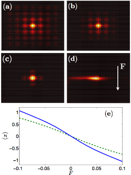
Figure 1: (a)-(d) Photon amplitude distribution $|a_{m,n}|$ on a $41\times 41$ square lattice with $\alpha=1/5$. The central sites are pumped. The force $F$ is zero for (a)-(c), and $F=0.1J$ for (d). In (a),(b),(d), the pump frequency is tuned to $\omega_{0}/J=-2.95$ within the lowest energy band; in (c), it is tuned to $\omega_{0}/J=-2.85$ within a band gap. The loss rate is $\gamma=0.01J$ for (a),(c),(d) and $\gamma=0.02J$ for (b). The bright regions have higher intensity than the dark regions. (e) Displacement $\langle x\rangle$ as a function of $F$, in units of $J$, for a pump frequency $\omega_{0}/J=-2.95$ with $\alpha=1/5$. The solid (blue) line is for $\gamma/J=0.05$, and the dashed (green) line is for $\gamma/J=0.08$.

We now proceed to relate the slope of this linear dependence to the topological properties of the band; a single band description is legitimate, provided the pump frequency $\omega_{0}$ falls within (or close to) an energy band and $\gamma$ is smaller than the band gap separating from the next bands. In the linear regime, this gives the simple relation between the displacement and the Berry curvature (a full proof of (3) as well as its extension to more complex - e.g., honeycomb - lattices is given in Supplemental Material)

$$\langle x\rangle=F\frac{\int_{\mathrm{MBZ}}\gamma\,\Omega(\mathbf{k})\,n(\mathbf{k})^{2}}{\int_{\mathrm{MBZ}}n(\mathbf{k})},$$ (3)

where $n(\mathbf{k})=[(\omega_{0}-\mathcal{E}(\mathbf{k}))^{2}+\gamma^{2}]^{-1}$ is the (normalized) population distribution within the band under consideration; $\mathcal{E}(\mathbf{k})$ and $\Omega(\mathbf{k})$ are the energy dispersion and the local Berry curvature, respectively, of the corresponding band.

The integral in (3) can be worked out explicitly in the two cases of large and small $\gamma$ as compared to the bandwidth of the energy band $\Delta_{\mathrm{width}}$; for large $\gamma\gg\Delta_{\mathrm{width}}$, one obtains the Chern numbers, and for small $\gamma\ll\Delta_{\mathrm{width}}$, one finds the Berry curvature. In practical experiments, the loss rate $\gamma$ can be tuned by artificially reducing the quality factor of the cavities or, alternatively, by tuning $\Delta_{\mathrm{width}}$ by varying the hopping amplitude $J$.

Large loss: Chern number and quantum Hall effect.— In the limit $\gamma\gg\Delta_{\mathrm{width}}$, the detuning term $[\omega_{0}-\mathcal{E}(\mathbf{k})]^{2}$ in $n(\mathbf{k})$ can be neglected, and a formula for the transverse shift is found:

$$\langle x\rangle \approx F\dfrac{\int_{\mathrm{MBZ}}d^{2}\mathbf{k}\,\Omega(\mathbf{k})/\gamma^{3}}{\int_{\mathrm{MBZ}}d^{2}\mathbf{k}\,1/\gamma^{2}}=\frac{q\mathcal{C}F}{2\pi\gamma}$$ (4)

that involves only the Chern number $\mathcal{C}$ of the band: This result is an optical analogue of the integer quantum Hall effect.

Of course, this formula is valid only if the loss rate $\gamma$ is much smaller than the band gap to the nearest energy band $\Delta_{\mathrm{gap}}$. This condition imposes a compromise between a large enough value of $\gamma/J$ to encompass the whole band of interest and a small enough value to minimize the spurious effect of the neighboring bands. For the lowest band of $\alpha=1/5$, the large separation from the higher bands ($\Delta_{\mathrm{gap}}/\Delta_{\mathrm{width}}\sim 24$) allows for a good compromise: By using $\gamma=2\Delta_{\mathrm{width}}$ and $\omega_{0}$ tuned at the band center, the estimated value $\mathcal{C}_{n}\approx-0.96$ of the Chern number is close to the exact value $\mathcal{C}=-1$.

As the leading order correction due to the neighboring bands to (4) does not depend on $\gamma$, a more precise estimate can be obtained by repeating the measurement on different samples with different values of the normalized loss rate $\gamma/J$ so as to extract the coefficient of $1/\gamma$ in (4). In Table 1, we list the estimated Chern numbers $\mathcal{C}_{n}$ obtained by numerically calculating the mean displacement $\langle x\rangle$ for different values of $\alpha$, and we compare them with the exact values $\mathcal{C}$ obtained from the Diophantine equation approach Bernevig2013 ; Thouless1982 . For each case, the pump frequency $\omega_{0}$ is chosen to be at the center of the band under examination, and the coefficient of the $1/\gamma$ term is calculated for a normalized loss value $\gamma/2J=(J/\Delta_{\mathrm{width}}+J/\Delta_{\mathrm{gap}})^{-1}$.

As long as the bandwidth is much larger than the band gap, the agreement is very good. On the other hand, the large deviation between the estimated and the exact Chern numbers of the second and fourth bands of $\alpha=1/5$ ($\mathcal{C}_{n}=-0.66$ instead of $\mathcal{C}=-1$ ) is because the corresponding bandwidth $\Delta_{\mathrm{width}}\sim 0.45J$ is very close to the size of the band gap $\Delta_{\mathrm{gap}}\sim 0.52J$. When $\Delta_{\mathrm{width}}>\Delta_{\mathrm{gap}}$, this method is not reliable at all, so the corresponding cases in the table have been left blank.

		1st	2nd	3rd	4th	5th	6th
$\alpha=\dfrac{1}{3}$	$\mathcal{C}$	$-1$	$+2$	$-1$
	$\mathcal{C}_{n}$	$-0.91$	-	$-0.91$
$\alpha=\dfrac{1}{5}$	$\mathcal{C}$	$-1$	$-1$	$+4$	$-1$	$-1$
	$\mathcal{C}_{n}$	$-0.97$	$-0.66^{*}$	-	$-0.66^{*}$	$-0.97$
$\alpha=\dfrac{1}{6}$	$\mathcal{C}$	$-1$	$-1$	$+2$	$+2$	$-1$	$-1$
	$\mathcal{C}_{n}$	$-0.96$	$-1.06$	-	-	$-1.06$	$-0.96$
$\alpha=\dfrac{3}{7}$	$\mathcal{C}$	$+2$	$-5$	$+2$	$+2$	$+2$	$-5$
	$\mathcal{C}_{n}$	$2.05$	-	-	$2.01$	-	-
$\alpha=\dfrac{4}{9}$	$\mathcal{C}$	$+2$	$+2$	$-7$	$+2$	$+2$	$+2$
	$\mathcal{C}_{n}$	$1.96$	-	-	$2.02$	$1.92$	$2.02$

Table 1: Table of the estimated Chern numbers $\mathcal{C}_{n}$ of the photonic bands, compared to the real Chern numbers $\mathcal{C}$, for several values of $\alpha$. The numerical estimations are obtained by implementing the method discussed in the text on $41\times 41$ square lattices. The blank cases indicate bands for which $\Delta_{\mathrm{width}}<\Delta_{\mathrm{gap}}$ where the method is not reliable; the $*$ signs indicate bands for which $\Delta_{\mathrm{width}}\simeq\Delta_{\mathrm{gap}}$ and large discrepancies are expected.

Small loss: Berry curvature and anomalous Hall effect.— When the loss $\gamma$ is much smaller than the bandwidth $\Delta_{\mathrm{width}}$, the $\mathbf{k}$-space distribution can be approximated as a delta function on the $\mathbf{k}$-space locus where $\omega_{0}\approx\mathcal{E}(\mathbf{k})$. In analogy to the (intrinsic contribution to the) anomalous Hall effect, the displacement

$$\langle x\rangle \approx F\gamma\bar{\Omega}(\omega_{0})\dfrac{\int_{\mathrm{MBZ}}d^{2}\mathbf{k}\,n(\mathbf{k})^{2}}{\int_{\mathrm{MBZ}}d^{2}\mathbf{k}\,n(\mathbf{k})}\approx\frac{\bar{\Omega}(\omega_{0})\,F}{2\gamma}$$ (5)

turns out to be proportional to the average $\bar{\Omega}(\omega_{0})$ of the Berry curvature on the $\mathcal{E}(\mathbf{k})=\omega_{0}$ curve in $\mathbf{k}$ space. Remarkably, different regions of the Brillouin zone can be separately addressed just by tuning the frequency $\omega_{0}$ of the coherent pump. In the case of the Hofstadter lattice, numerical calculations suggest that the Berry curvature is a function of the energy only, so a reliable estimate of the local Berry curvature at the different points of the MBZ can be obtained from a measurement of $\bar{\Omega}(\omega_{0})$ provided only the iso-$\mathcal{E}$ locus in $\mathbf{k}$ space does not cross stationary points of $\mathcal{E}(\mathbf{k})$.

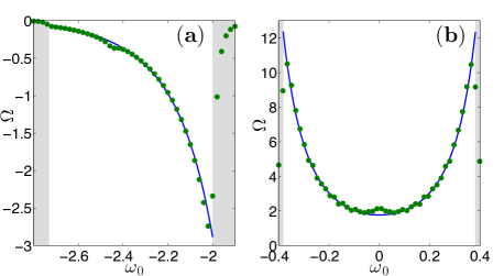
Figure 2: The estimated Berry curvature $\Omega$ as a function of $\omega_{0}$, in units of $J$ (dots) as compared to the exact value (solid lines) for $\gamma/\Delta_{\mathrm{width}}=1/30$ on $201\times 201$ lattices. (a) Lowest band of square lattice at $\alpha=1/3$ and (b) middle band of square lattice at $\alpha=1/5$.

The accuracy of this result is validated in Fig. 2, where we plot the estimated value of the Berry curvature for the lowest band of $\alpha=1/3$ and the central band of $\alpha=1/5$, and we compare them with the true values. The loss rate is taken here to be $\gamma/\Delta_{\mathrm{width}}=1/30$; for such a small value of $\gamma$, photons propagate over longer distances before decaying, so larger lattices are needed to suppress the effect of the edges. Overall, the estimated value of the Berry curvature agrees well with its exact value for almost all values of the pump frequency $\omega_{0}$ in the bulk of the bands. Of course, the method breaks down in the vicinity of the band edges and becomes meaningless within the energy gaps (indicated by the gray shading in the figure). But note also the small spurious bumps around $\omega_{0}/J\sim-2.45$ for $\alpha=1/3$ and $\omega_{0}/J\sim 0$ for $\alpha=1/5$: These deviations correspond to stationary points of the band structure $\mathcal{E}(\mathbf{k})$ where the last equality of (5) is no longer valid. The quantitative discrepancy gets suppressed if smaller values of $\gamma$ are used. It is, however, important to notice that, since our scheme does not benefit from topological protection, the actual measured displacement $\langle x\rangle$ can be affected by disorder. To suppress the deleterious effect of disorder, one may repeat the measurement by choosing different lattice sites for the pumping and then taking an average.

Photonic honeycomb lattice.— As a last point, we discuss the nontrivial new features that arise when extending our study to honeycomb lattices. We consider the usual tight-binding model of the honeycomb lattice sketched in Fig. 3(a), with a nearest-neighbor hopping $J$ which is now real and equal for all links CastroNeto2009 . The unit vectors are $\mathbf{a}_{1}\equiv(3/2,\sqrt{3}/2)$ and $\mathbf{a}_{2}\equiv(3/2,-\sqrt{3}/2)$, where the distance between two sites is taken to be unity. In the presence of a small energy difference $\Delta$ between the sublattices, the band degeneracy at the Dirac points $\mathbf{K,~{}K^{\prime}}=2\pi(1/3,\pm 1/3\sqrt{3})$ is lifted by a band gap $\Delta$, and the two bands have a nontrivial Berry curvature even in the absence of a synthetic magnetic field Xiao2007 ; as illustrated in Fig. 3(b), the Berry curvature is concentrated in the vicinity of the (gapped) Dirac points, and, for each band, it is approximately a function of the energy only. As a result of the time-reversal symmetry, the Berry curvatures at $\mathbf{K}$ and $\mathbf{K}^{\prime}$ exactly compensate giving a vanishing global Chern number for both bands and therefore no quantum Hall effect. As the averaged Berry curvature vanishes on any isoenergy curve, extension of the analogue anomalous Hall effect to honeycomb geometries requires separating the contributions of the $\mathbf{K}$ and $\mathbf{K}^{\prime}$ points.

Figure 3: (a) Photonic honeycomb lattice. Sites belonging to the sublattices $A$ and $B$ are denoted by empty and filled circles, respectively. (b) The Berry curvature of the upper band of a honeycomb lattice with $\Delta=0.3J$. The Dirac points are the vertices of the hexagon. (c) The estimated Berry curvature $\Omega$ as a function of $\omega_{0}$, in units of $J$ (dots) as compared to the exact value (solid line), for the honeycomb lattice without a synthetic magnetic field. System parameters are $\gamma/J=0.04$ and $\sigma=3$ on a $200\times 200$ unit cell honeycomb lattice with site energy mismatch $\Delta/J=0.3$. The shaded region indicates the band gap.

The simplest strategy in this direction is to use a spatially extended pump with a finite in-plane wave vector in the vicinity of, e.g., the $\mathbf{K}$ point:

$$f({\mathbf{R}})=f\,e^{-{R}^{2}/2\sigma^{2}}e^{i\mathbf{K}\cdot\mathbf{R}},$$ (6)

where $\sigma$ is the spatial extent of the pump spot and $\mathbf{R}$ is the position of each site. In the experimental setup of Ref. AmoPC , this can be obtained by shining a laser field on the microcavity at a finite and well-chosen angle with the microcavity axis Carusotto2013 . As before, the basic idea is to find out how the Berry curvature controls the transverse displacement of the intensity distribution when an in-plane force is applied to the photons.

While doing this, one has to deal with further complications stemming from the inequivalence of the two sublattices: As a result of this, measurements using a pump in the form (6) would in fact lead to nonzero displacements even for $F=0$ and to a slope not directly related to the Berry curvature. All these difficulties can be resolved by repeating the measurement using two different, symmetric frequencies $\pm\omega_{0}$ and taking a weighted difference of the two measured displacements:

$$\langle x\rangle_{-} \equiv\frac{\sum_{\mathbf{R}}R_{x}(|a_{\mathbf{R}}|^{2}-|a^{\prime}_{\mathbf{R}}|^{2})}{\sum_{\mathbf{R}}(|a_{\mathbf{R}}|^{2}+|a^{\prime}_{\mathbf{R}}|^{2})},$$ (7)

where $a_{\mathbf{R}}$ is the photon field at position $\mathbf{R}$ when the pump frequency is $\omega_{0}$ and $a^{\prime}_{\mathbf{R}}$ is when the frequency is $-\omega_{0}$. With this definition of $\langle x\rangle_{-}$, a straightforward analytical calculation (see the Supplemental Material for details and also for an alternative strategy to measure the Berry curvature right at the tip of the gapped Dirac cone) shows that the formula (3) holds with the integral taken over the Brillouin zone and the integrand being multiplied by the Fourier transform of the source. Then, using a source which uniformly covers the vicinity of $\mathbf{K}$ but is very small near other Dirac cones, one can estimate the Berry curvature from the transverse shift using the anomalous Hall effect formula (5). The accuracy of this method is validated in Fig. 3(c), where we plot the estimated value of the Berry curvature using this method for the region around the $\mathbf{K}$ Dirac point; agreement with the theoretical value (solid line) is very good.

Conclusion.— In this Letter, we have discussed optical analogues of the anomalous and integer quantum Hall effects in driven-dissipative photonic lattices with nontrivial geometrical and topological properties. Our results suggest that both the Chern number and the local Berry curvature of the photonic bands can be experimentally extracted from the transverse displacement of the light distribution under the effect of an additional force and support the promise of photonic cavity arrays as a platform to study the interplay of the nontrivial band topology with many-body physics.

- (1) I. Carusotto and C. Ciuti, Rev. Mod. Phys. 85, 299 (2013).
- (2) J. Kasprzak, M. Richard, S. Kundermann, A. Baas, P. Jeambrun, J. M. J. Keeling, F. M. Marchetti, M. H. Szymańska, R. André, J. L. Staehli, V. Savona, P. B. Littlewood, B. Deveaud, and L. S. Dang, Nature (London) 443, 409 (2006).
- (3) A. Amo, J. Lefrère, S. Pigeon, C. Adrados, C. Ciuti, I. Carusotto, R. Houdré, E. Giacobino, and A. Bramati, Nature Physics 5, 805 (2009).
- (4) F. D. M. Haldane and S. Raghu, Phys. Rev. Lett. 100, 013904 (2008).
- (5) Z. Wang, Y. Chong, J. D. Joannopoulos, and M. Soljačić, Nature (London) 461, 772 (2009).
- (6) M. C. Rechtsman, J. M. Zeuner, Y. Plotnik, Y. Lumer, D. Podolsky, F. Dreisow, S. Nolte, M. Segev, and A. Szameit, Nature 496, 196 (2013).
- (7) M. C. Rechtsman, J. M. Zeuner, A. Tünnermann, S. Nolte, M. Segev, and A. Szameit, Nature Photonics 7, 153 (2013).
- (8) M. Hafezi, J. Fan, A. Migdall, and J. Taylor, Nature Photonics 7, 1001 (2013).
- (9) N. Jia, A. Sommer, D. Schuster, and J. Simon, arXiv:1309.0878.
- (10) M. Z. Hasan and C. L. Kane, Rev. Mod. Phys. 82, 3045 (2010).
- (11) X.-L. Qi and S.-C. Zhang, Rev. Mod. Phys. 83, 1057 (2011).
- (12) B. A. Bernevig and T. L. Hughes, Topological Insulators and Topological Superconductors (Princeton University, Princeton, NJ, 2013).
- (13) A. Stern, Ann. Phys. (N.Y.) 323, 204 (2008).
- (14) J. Cho, D. G. Angelakis, and S. Bose, Phys. Rev. Lett. 101, 246809 (2008).
- (15) R. O. Umucalılar and I. Carusotto, Phys. Rev. Lett. 108, 206809 (2012).
- (16) M. Hafezi, M. D. Lukin, and J. M. Taylor, New J. Phys. 15, 063001 (2013).
- (17) M. Hafezi, E. A. Demler, M. D. Lukin, and J. M. Taylor, Nature Physics 7, 907 (2011).
- (18) K. Fang, Z. Yu, and S. Fan, Nature Photonics 6, 782 (2012).
- (19) R. B. Laughlin, Phys. Rev. B 23, 5632 (1981).
- (20) D. J. Thouless, M. Kohmoto, M. P. Nightingale, and M. den Nijs, Phys. Rev. Lett. 49, 405 (1982).
- (21) Y. Hatsugai, Phys. Rev. Lett. 71, 3697 (1993).
- (22) D. Xiao, M.-C. Chang, and Q. Niu, Rev. Mod. Phys. 82, 1959 (2010).
- (23) M.-C. Chang and Q. Niu, Phys. Rev. B 53, 7010 (1996).
- (24) N. Nagaosa, J. Sinova, S. Onoda, A. H. MacDonald, and N. P. Ong, Rev. Mod. Phys. 82, 1539 (2010).
- (25) A. M. Dudarev, R. B. Diener, I. Carusotto, and Q. Niu, Phys. Rev. Lett. 92, 153005 (2004).
- (26) G. Pettini and M. Modugno, Phys. Rev. A 83, 013619 (2011).
- (27) H. M. Price and N. R. Cooper, Phys. Rev. A 85, 033620 (2012).
- (28) D. A. Abanin, T. Kitagawa, I. Bloch, and E. Demler, Phys. Rev. Lett. 110, 165304 (2013).
- (29) E. Alba, X. Fernandez-Gonzalvo, J. Mur-Petit, J. K. Pachos, and J. J. Garcia-Ripoll, Phys. Rev. Lett. 107, 235301 (2011).
- (30) A. Dauphin and N. Goldman, Phys. Rev. Lett. 111, 135302 (2013).
- (31) M. Cominotti and I. Carusotto, Europhys. Lett. 103 10001 (2013).
- (32) T. Jacqmin, I. Carusotto, I. Sagnes, M. Abbarchi, D. Solnyshkov, G. Malpuech, E. Galopin, A. Lemaître, J. Bloch, and A. Amo, arXiv:1310.8105.
- (33) D. Xiao, W. Yao, and Q. Niu, Phys. Rev. Lett. 99, 236809 (2007).
- (34) A. H. Castro Neto, N. M. R. Peres, K. S. Novoselov, and A. K. Geim, Rev. Mod. Phys. 81, 109 (2009).
- (35) P. G. Harper, Proc. Phys. Soc. London Sect. A 68, 874 (1955).
- (36) D. R. Hofstadter, Phys. Rev. B 14, 2239 (1976).