Efficient simulation of the random-cluster model

Abstract

The simulation of spin models close to critical points of continuous phase transitions is heavily impeded by the occurrence of critical slowing down. A number of cluster algorithms, usually based on the Fortuin-Kasteleyn representation of the Potts model, and suitable generalizations for continuous-spin models have been used to increase simulation efficiency. The first algorithm making use of this representation, suggested by Sweeny in 1983, has not found widespread adoption due to problems in its implementation. However, it has been recently shown that it is indeed more efficient in reducing critical slowing down than the more well-known algorithm due to Swendsen and Wang. Here, we present an efficient implementation of Sweeny’s approach for the random-cluster model using recent algorithmic advances in dynamic connectivity algorithms.

I Introduction

In the vicinity of a continuous phase transition, particle or spin systems of statistical mechanics develop extended spatial correlations signaling the onset of long-range translational order through spontaneous symmetry breaking. It has been realized early on that these phenomena suggest a description of the ordering in geometrical terms, using analogies to the percolation transition Fisher (1967). While Fisher’s droplet model initially considered simple clusters of like spins (geometrical clusters) as the relevant quantities, it was only gradually realized in the 1980s that the relevant collective degrees of freedom, or “physical clusters”, are indeed of a different nature, and they can be constructed by breaking the geometric clusters up following a suitable stochastic prescription activating bonds within clusters with probability $p=1-\exp(-J/k_{B}T)<1$ Coniglio and Klein (1980). Initially, this breakup was only applied to one spin species (of the Ising model, say), leading to inconsistencies in the symmetric high-temperature phase. It was in an independent line of thought by Fortuin and Kasteleyn Fortuin and Kasteleyn (1972); *fortuin:72b; *fortuin:72c that an equivalence of the partition function of the $q$-state Potts model Wu (1982) to a correlated bond-percolation problem known as the random-cluster model with partition function

$$Z_{\mathrm{RC}}=\sum_{{\cal G}^{\prime}\subseteq{\cal G}}v^{b({\cal G}^{\prime})}q^{n({\cal G}^{\prime})}$$ (1)

was established. Here, ${\cal G}^{\prime}$ denotes the set of $b({\cal G}^{\prime})$ activated edges on a lattice graph ${\cal G}$, resulting in $n({\cal G}^{\prime})$ connected components, and the bond weight $v=p/(1-p)$. These results led Hu Hu (1984) to generalize the above bond activation probability to all geometric clusters irrespective of their orientation. As a consequence, the right choice of physical droplets is now well understood, and the equivalence of their percolation properties and thermal quantities has been explicitly checked De Meo et al. (1990).

The growth without bounds of static correlations in critical systems is accompanied in the time domain by a divergence of relaxation times known as critical slowing down Hohenberg and Halperin (1977). While this is a physical phenomenon connected, for instance, to the effect of critical opalescence, it is also of direct relevance for the pseudo-dynamics in Monte Carlo simulations of near-critical systems. As this leads to an asymptotic inefficiency of Markov chain Monte Carlo in producing independent samples, an improved understanding of spatial correlations was hoped to translate into suitable non-local updating procedures allowing to precisely study near-critical systems. Initial attempts in this direction, such as variants of the multi-grid approach Schmidt (1983); Goodman and Sokal (1986), were based on renormalization group ideas, and turned out to be only moderately successful. The first Monte Carlo algorithm based on the concept of physical clusters was suggested by Sweeny in 1983 Sweeny (1983). He considered a direct simulation of the bond variables of Eq. (1), randomly suggesting state switches from active to inactive and vice versa. As the relevant Boltzmann weight depends on the number $n({\cal G}^{\prime})$ of connected components resulting from a given bond configuration, calculating the acceptance probability of the bond moves needs up-to-date information about cluster connectivity. Hence, a single update might require the expensive traversal of large (possibly spanning) clusters, potentially destroying the computational advantage of an accelerated decorrelation of configurations through computational critical slowing down Deng et al. (2010).

An alternative suggestion made by Swendsen and Wang Swendsen and Wang (1987) works directly on the spin configuration, freezing bonds between like spins with probability $p=1-\exp(-J/k_{B}T)$ and independently flipping the resulting spin clusters. Instead of working in the graph language alone, this series of alternating updates of spin and bond variables corresponds to a Markov chain in an augmented state space Edwards and Sokal (1988). The resulting algorithm (with its many variants including, for instance, the single-cluster version Wolff (1989)) is rather straightforward to implement and turns out to be very efficient in beating critical slowing down, reducing the dynamical critical exponent, e.g., of the 2D Ising model from $z\approx 2$ for local spin flips to $z\approx 0.2$ Garoni et al. (2011). Owing to this success of the Swendsen-Wang algorithm and related techniques as well as the delicacies of maintaining up-to-date connectivity information, Sweeny’s approach was not used by many researchers. Also, its reduction of critical slowing down was not precisely investigated until, about 20 years after the original work, it was claimed that a variant of the single-bond algorithm was completely free of critical slowing down Gliozzi (2002). Although this was later shown to be incorrect Wang et al. (2002), it was not until recently that its dynamical critical behavior was investigated in more detail Qian et al. (2005a); Deng et al. (2007a), revealing the surprising feature of critical speeding up, i.e. $z<0$, for certain ranges of $q$ alongside generally smaller dynamical critical exponents than those found for the Swendsen-Wang dynamics.

Besides it being a very elegant and direct sampling procedure for the weights of Eq. (1), another favorable feature of Sweeny’s approach is its general applicability to arbitrary values of $q$: while the Potts model is only defined for integer $q=1$, $2$, $3$, $\ldots$, the random cluster model of Eq. (1) is meaningful for any real value $q\geq 0$, serving as an analytic continuation of the Potts model to real $q$ Grimmett (2006). The Swendsen-Wang algorithm, originally working with a joint spin and bond representation meaningful only for integer $q$, can be generalized to non-integer $q\geq 1$ Chayes and Machta (1998). The bond algorithm, however, is the only approach for $0<q<1$. This fact has prompted a number of researchers to use Sweeny’s approach to probe the $q<1$ regime, for instance to study fractal properties of the cluster structure Qian et al. (2005b); Zatelepin and Shchur (2010); Gliozzi and Rajabpour (2010). The main obstacle to a more widespread adoption, however, has been the problem of expensive connectivity checks: inserting an edge might join two previously unconnected clusters, deleting a bond can lead to cluster fragmentation. A naive approach without additional data structures appears to require the tracing out of one (or two) randomly chosen cluster(s) to check for connectivity. As the average cluster size scales proportional to $L^{\gamma/\nu}$ Stauffer and Aharony (1994) and $\gamma/\nu\geq 1.75$ for the random-cluster model, the cost of a full lattice sweep is almost squared as compared to single spin flips or Swendsen-Wang. In his paper, Sweeny had suggested a specific solution for the case of two-dimensional lattices, replacing the traversal of clusters with a tracking of boundary loops on the medial lattice Sweeny (1983); Deng et al. (2010). Irrespective of space dimension, a pair of interleaved breadth-first searches starting from both ends of the bond currently examined can also dramatically improve the situation Weigel (2010); Deng et al. (2010). While these connectivity algorithms still exhibit power-law scaling with the size of the system, fully dynamic connectivity algorithms, where edge insertions and removals can be performed in amortized times at most (poly)logarithmic in the system size, are known in computer science Henzinger and King (1999); Holm et al. (2001). Here, we compare a number of different implementations of Sweeny’s algorithm for simulations of the random-cluster model to each other as well as to the Chayes-Machta-Swendsen-Wang dynamics Swendsen and Wang (1987); Chayes and Machta (1998). The combination of a polylogarithmic dynamic connectivity algorithm and Sweeny’s single-bond approach is shown to be the more efficient way, asymptotically, to simulate the random-cluster model at criticality.

The rest of the paper is organized as follows. In Sec. II, we introduce Sweeny’s algorithm in more detail and describe the three different variants of connectivity checks implemented here: breadth-first search, union-and-find, and dynamic connectivities. Section III contains an in-depth comparison of the scaling of properties of these approaches as compared to the Chayes-Machta-Swendsen-Wang dynamics in terms of simulation as well as computer time for the case of simulations on the square lattice. Finally, Sec. IV contains our conclusions.

II Model and algorithms

The random-cluster model (RCM) assigns weights to (spanning) sub-graph configurations ${\cal G}^{\prime}$, i.e., subsets of activated edges and the complete set of vertices, of the underlying graph ${\cal G}$ according to Grimmett (2006)

$$w_{\mathrm{RC}}({\cal G}^{\prime})=q^{n({\cal G}^{\prime})}v^{b({\cal G}^{\prime})},$$ (2)

leading to the partition sum of Eq. (1). For integer values of the cluster weight $q$, the partition function (1) is identical Fortuin and Kasteleyn (1972) to that of the $q$-state Potts model with Hamiltonian

$${\cal H}=-J\sum_{b\in{\cal G}}\delta_{\sigma_{i},\sigma_{j}},$$ (3)

where $b=(i,j)$ is an edge in the graph ${\cal G}$, and $\sigma_{i}\in\{1,\ldots,q\}$. For the purposes of this study, we will restrict ourselves to graphs in two dimensions (2D), namely compact $L\times L$ regions of the square lattice, applying periodic boundary conditions. For this case, the ordering transition of the Potts model occurs at the coupling $J/k_{B}T=\ln(1+\sqrt{q})$, corresponding to the critical bond weight $v_{c}=\sqrt{q}$ in (1). This transition is continuous for $q\leq 4$ and first-order for $q>4$ Wu (1982).

II.1 Sweeny’s algorithm

Starting from the results of Fortuin and Kasteleyn Fortuin and Kasteleyn (1972), Sweeny suggested to directly sample bond configurations of the RCM according to the weight (2). For any sub-graph ${\cal G}^{\prime}$, the basic update operation is then given by the deletion of an occupied edge or the insertion of an unoccupied edge. According to Eq. (2), the corresponding transition probabilities depend on the changes $\Delta b$ of the number of active edges and $\Delta n$ of the number of connected components or clusters. While $\Delta b$ is trivially determined to equal $+1$ for edge insertion and $-1$ for edge removal, respectively, the change in cluster number depends on whether a chosen inactive edge is internal to one cluster ($\Delta n=0$) or, instead, it is external and hence amalgamates two existing clusters if activated ($\Delta n=-1$). Likewise, removing an edge might lead to $\Delta n=0$ or $\Delta n=+1$, depending on whether an alternative path exists connecting the end points of the removed edge. The construction and implementation of data structures supporting the efficient calculation of $\Delta n$ constitutes the intricacy of Sweeny’s algorithm and the focus of the present work.

Importance sampling for the weight (2) can be constructed along well-known lines, the most common choices being the heat-bath and Metropolis schemes Binder and Landau (2009). In both cases, a bond is randomly and uniformly selected from the graph and a “flip” of its occupation state from inactive to active or vice versa is proposed. The heat-bath acceptance ratio, used in the original approach of Sweeny Sweeny (1983) is then given by

$$p_{\mathrm{acc}}^{\mathrm{HB}}(\Delta b,\Delta n)=\frac{q^{\Delta n}v^{\Delta b}}{1+q^{\Delta n}v^{\Delta b}}.$$ (4)

For Metropolis-Hastings, on the other hand, we have

$$p_{\mathrm{acc}}^{\mathrm{MH}}(\Delta b,\Delta n)=\min(1,q^{\Delta n}v^{\Delta b}).$$ (5)

It is easily seen that

$$\frac{1}{2}\leq\frac{p_{\mathrm{acc}}^{\mathrm{HB}}}{p_{\mathrm{acc}}^{\mathrm{MH}}}=\frac{\max(1,q^{\Delta n}v^{\Delta b})}{1+q^{\Delta n}v^{\Delta b}}<1.$$

Depending on $q$ and $v$, we hence expect up to twice larger acceptance rates for the Metropolis variant. At criticality, $v=\sqrt{q}$, the minimal ratio $p_{\mathrm{acc}}^{\mathrm{HB}}/p_{\mathrm{acc}}^{\mathrm{MH}}=1/2$ is reached in the percolation limit $q=1$. In contrast to Ref. Sweeny (1983), our numerical experiments concentrate on Metropolis acceptance.

As, depending on the data structures used, the determination of the change $\Delta n$ in cluster number is the most expensive operation, it is economic to only determine $\Delta n$ if it is actually required for the update. In an update attempt, one draws a random number uniformly in $[0,1[$; if $r\leq p_{\mathrm{acc}}$ the move is accepted, otherwise it is rejected. Given that

$$r\leq\min_{\Delta n}\,p_{\mathrm{acc}}(\Delta b,\Delta n),$$

where $\Delta n\in\{0,\,-1\}$ for insertion and $\Delta n\in\{0,\,+1\}$ for deletion, respectively, the move can be unconditionally accepted Gliozzi (2002). Conversely, for

$$r>\max_{\Delta n}\,p_{\mathrm{acc}}(\Delta b,\Delta n)$$

unconditional rejection occurs. At criticality, $v=\sqrt{q}$, this results in a fraction

$$\min(\sqrt{q},1/\sqrt{q})$$

of moves which can be unconditionally accepted or rejected under the Metropolis dynamics . Likewise, for the heat-bath rate (4), a fraction

$$\frac{2}{1+\sqrt{q}}\,\min(1,\sqrt{q})$$

of move attempts can be decided without actually working out $\Delta n$. Note that, in both cases, these fractions tend to unity as $q\to 1$ which is a result of the cluster weight (2) becoming independent of cluster number in the uncorrelated percolation limit. Connectivity checks are hence never required there.

II.2 Connectivity algorithms

The main complication for an efficient implementation of the bond algorithm is to maintain the full connectivity information of the current sub-graph. Consider a flip attempt on a random edge; it can be currently in the active or inactive (inserted or deleted) state. For each of these cases, one needs to distinguish internal from external edges, such that independent paths connecting the two end points either exist (internal edge) or are absent (external edge). This leads to the four cases of internal/external insertions/deletions, each of which can exhibit rather different runtime scaling behavior depending on the chosen implementation.

II.2.1 Breadth-first search

Table 1: Asymptotic run-time scaling at criticality of the elementary operations of insertion or deletion of internal or external edges, respectively, using sequential breadth-first search (SBFS), interleaved BFS (IBFS), union-and-find (UF) or the fully dynamic connectivity algorithm (DC) as a function of the linear system size $L$.

move	SBFS	IBFS	UF	DC
internal insertion	$L^{d_{F}-x_{2}}$	$L^{d_{F}-x_{2}}$	const.	$\log^{2}L$
external insertion	$L^{\gamma/\nu}$	$L^{d_{F}-x_{2}}$	const.	$\log^{2}L$
internal deletion	$L^{d_{F}-x_{2}}$	$L^{d_{F}-x_{2}}$	$L^{d_{F}-x_{2}}$	$\log^{2}L$
external deletion	$L^{\gamma/\nu}$	$L^{d_{F}-x_{2}}$	$L^{\gamma/\nu}$	$\log^{2}L$
dominant	$L^{\gamma/\nu}$	$L^{d_{F}-x_{2}}$	$L^{\gamma/\nu}$	$\log^{2}L$

The simplest approach to the connectivity problem is to not maintain any state information about clusters and determine the value of $\Delta n$ for each individual bond move from direct searches in the graph structure around the current edge $e=(i,j)$. Such traversals are most naturally implemented as breadth-first search (BFS) Cormen et al. (2009) starting from one of the end-points, say $i$, while not being allowed to cross the edge $e$. In case of an external edge, the cluster attached to $i$ needs to be fully traversed. For an internal edge, on the other hand, the search starting at $i$ terminates once it arrives at $j$, having found an alternative path connecting $i$ and $j$. Instead of the BFS one could also use a depth-first search (DFS) to achieve the same result Cormen et al. (2009). We found essentially no differences in the run-time behavior of both variants, however, and hence did not consider this possibility in more detail. To determine the asymptotic run-time at criticality of these operations, we note that the average number of clusters with mass $s$ per lattice site is Stauffer and Aharony (1994)

$$n_{s}\sim s^{-\tau}e^{-cs},$$ (6)

where $\tau$ is the cluster-size or Fisher exponent. A randomly picked site will therefore, on average, belong to a cluster of size

$$M_{2}=\sum_{s}s^{2}n_{s}\sim\int s^{2-\tau}e^{-cs}\propto c^{\tau-3}\sim L^{(\tau-3)/\sigma\nu},$$

where the last identity follows from $c\sim|p-p_{c}|^{1/\sigma}$ and the standard finite-size scaling ansatz $|p-p_{c}|\sim L^{1/\nu}$. Since $(3-\tau)/\sigma=\gamma$, we arrive at a typical cluster size $M_{2}\sim L^{\gamma/\nu}$ Stauffer and Aharony (1994). For operations on external edges, we therefore expect an asymptotic scaling of run-times $\sim L^{\gamma/\nu}$. For internal edges, on the other hand, the relevant effort corresponds to the total number of visited sites of a breadth-first search starting from site $i$ until it reaches $j$. In this case, the number of shells $\ell$ in the BFS at termination is just the shortest path between $i$ and $j$. As shown by Grassberger Grassberger (1992a, 1999), for bond percolation, the probability of two nearby points on the lattice to be connected by a shortest path of length $\ell$ is $p(\ell)\sim l^{-\psi_{\ell}}\mathcal{L}(\ell/L^{d_{\mathrm{min}}})$, where

$$\psi_{\ell}=1+\frac{2\beta}{\nu d_{\mathrm{min}}}+\frac{g_{1}}{d_{\mathrm{min}}}.$$

Here, $d_{\mathrm{min}}$ is the shortest-path fractal dimension Grassberger (1992b) and $g_{1}$ is the scaling exponent related to the density of growth sites Grassberger (1999). Ziff Ziff (1999) demonstrated that $g_{1}=x_{2}-2\beta/\nu$, where $x_{2}$ is the two-arm scaling exponent Cardy (1998); Smirnov and Werner (2001). Hence $\psi_{\ell}=1+x_{2}/d_{\mathrm{min}}$. As a result, the average length of shortest path between nearby points exhibits system-size scaling according to

$$\langle\ell\rangle\sim L^{d_{\mathrm{min}}-x_{2}}.$$ (7)

The number of sites touched by a BFS from $i$ to $j$ separated by a shortest path of length $\ell$ is expected to be $\ell^{\hat{d}}$, where $\hat{d}=d_{F}/d_{\mathrm{min}}$ is known as spreading dimension Grassberger (1992b). Here, $d_{F}=d-\beta/\nu$ denotes the fractal dimension of the percolating cluster. Hence, the average number of sites touched by the BFS for an internal edge is

$$\langle\ell^{\hat{d}}\rangle\sim L^{d_{F}-x_{2}}.$$ (8)

Note that, while $d_{F}$ and $x_{2}$ are exactly known Nienhuis (1987); Stauffer and Aharony (1994), this is not the case for $d_{\mathrm{min}}$ Deng et al. (2010); Zhou et al. (2012).

The asymptotic run-time scaling of the Sweeny update using sequential BFS (SBFS) hence depends on the fractions of internal and external edges encountered. These are found to be asymptotically $L$ independent numbers $0<r_{\mathrm{int}},r_{\mathrm{ext}}<1$ which, however, vary with $q$ Gyure and Edwards (1992); Elçi and Weigel . Comparing the scaling exponents for the operations on internal and external edges, it is found that $\gamma/\nu>d_{F}-x_{2}$ for the whole range $0\leq q\leq 4$, cf. the data compiled in Table 3. As a consequence, the stronger scaling $\sim L^{\gamma/\nu}$ of the operations on external edges will always dominate the running time in the limit of large system sizes.

An improvement suggested in Refs. Weigel (2002, 2010); Deng et al. (2010) concerns the quasi simultaneous execution of both BFSs. In practice, no hardware-level parallelism is needed here and, instead, sites are removed from the BFS queues of the two searches in an alternating fashion, effectively leading to an interleaved structure of the cluster traversals. To understand the benefit of this modification, consider the insertion of an edge $e$. If it is external, $i$ and $j$ belong to separate clusters ${\cal C}_{1}$ and ${\cal C}_{2}$ after the deletion of $e$. In this case, the searches terminate as soon as the smaller of the two clusters has been exhausted, i.e., after $C_{2,\mathrm{min}}\equiv\min(|{\cal C}_{1}|,|{\cal C}_{2}|)$ steps. Deng et al. Deng et al. (2010) have shown that, at criticality, this minimum scales as $L^{d_{F}-x_{2}}$, i.e., with the exponent already found above for operations on internal edges in SBFS. For the case of an internal edge, the interleaved searches terminate as soon as they meet each other. As argued in Ref. Deng et al. (2010) this time again exhibits the same run-time scaling $\sim L^{d_{F}-x_{2}}$ which is hence the relevant asymptotic behavior of the critical bond algorithm using interleaved BFS (IBFS). In Table 1 we compare the run-time scaling of the elementary operations between the different implementations of connectivity checks considered here.

II.2.2 Union-and-find

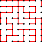
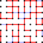
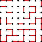
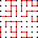
Figure 1: (Color online) Equilibrium bond configurations for a $L=8$ system at criticality, $v_{c}=\sqrt{q}$. The left (right) column shows a configuration for $q=0.0005$ ($q=2$). The first (second) row corresponds to the level $0$ ($1$) graph. Here, tree edges are indicated in red, solid lines, while non-tree edges are drawn with blue, dotted lines.

Sequential amalgamations of clusters through the addition of bonds can be handled efficiently using tree-based data structures under a paradigm known as union-and-find. This is traditionally applied to set partitioning Cormen et al. (2009), but has also been used in lattice models for highly efficient simulations of the bond percolation problem Newman and Ziff (2001). Each cluster is represented as a directed tree of nodes with pointers to their parent nodes; the root corresponds to a designated site representing the cluster as a whole. In this data structure, connectivity queries are answered by path traversal to the root sites, such that two sites are connected if and only if they have the same root. Using path compression Cormen et al. (2009), where (most of) the node pointers directly link to the cluster root, as well as a balancing heuristic that attaches the smaller cluster to the root of the bigger in case of cluster fusion, allows to perform the connectivity check with a worst-time scaling practically indistinguishable from a constant Tarjan (1975).

Table 2: Estimated dynamical critical exponents $z_{\mathrm{int},{\cal O}}$ for the two-dimensional RCM at criticality and ${\cal O}=\mathcal{S}_{2}$ as well as ${\cal O}=\mathcal{N}$ for a range of $q$ values as compared to results reported in Refs. Deng et al. (2007a, b); Garoni et al. (2011). The values shown for $z_{\mathrm{int},\mathcal{S}_{2}}^{\mathrm{SW}}$ for the Swendsen-Wang-Chayes-Machta algorithm are actually related to another observable $\mathcal{E}$, but it was reported in Refs. Deng et al. (2007b); Garoni et al. (2011) that the observables $\mathcal{E}^{\prime}$, ${\cal N}$ and ${\cal S}_{2}$ share the same dynamical critical exponent for this algorithm.

$q$	$z_{\mathrm{int},\mathcal{S}_{2}}$	$z_{\mathrm{int},\mathcal{S}_{2}}$ Deng et al. (2007a)	$z_{\mathrm{int},\mathcal{S}_{2}}^{\mathrm{SW}}$ Deng et al. (2007b); Garoni et al. (2011)	$z_{\mathrm{int},\mathcal{N}}$	$\alpha/\nu$	$z_{\mathrm{int},\mathcal{N}}$ Deng et al. (2007a)	$z_{\mathrm{int},\mathcal{S}_{2}}^{\mathrm{SW}}-z_{\mathrm{int},\mathcal{S}_{2}}$
0.0005	$-1.12(1)$	-1.23	—	$0.01(1)$	-1.958	0	—
0.005	$-1.09(1)$	-1.21	—	$0.01(1)$	-1.868	0	—
0.05	$-1.04(1)$	-1.12	—	$0.01(1)$	-1.601	0	—
0.2	$-0.86(1)$	-1.01	—	$-0.01(1)$	-1.247	0	—
0.5	$-0.63(1)$	-0.71	—	$0.00(1)$	-0.878	0	—
1.0	$-0.33(1)$	-0.32	—	$0.00(1)$	-0.500	0	—
1.5	$-0.11(2)$	-0.16	0	$0.06(2)$	-0.227	0
2.0	$0.03(3)$	-0.08	0.143(3)	$0.13(2)$	0	0 (log)	0.11
3.0	$0.44(4)$	0.41	0.497(3)	$0.45(4)$	0.400	0.45(1)	0.06
4.0	$0.75(6)$	—	0.910(5)	$0.73(6)$	1	—	0.16

Using this data structure for an implementation of the bond algorithm for the RCM Elçi (2011), edge insertion requires a connectivity check. If the edge is identified as internal, the cluster structure remains unchanged on its insertion which hence can be performed in constant time. For an external edge, insertion is realized through the attachment of the cluster root of the smaller cluster to the bigger which is, again, a constant-time operation. For the deletion of an edge $e=(i,j)$, the information about alternate paths between $i$ and $j$ is not directly contained in the data structure. We hence use interleaved BFS to detect such paths, with a computational effort asymptotically proportional to $L^{d_{F}-x_{2}}$. For an internal edge, this completes the deletion. For the case of an external edge, leading to fragmentation of the original cluster, a complete re-labeling of both new clusters is required, however, resulting in a total scaling of $\sim L^{\gamma/\nu}$ for this step, cf. Table 1.

The total effective runtime of a bond simulation with union-and-find data structure depends on the frequency of the individual operation types. The average number of active bonds at criticality can be worked out from results for the square-lattice Potts model, where the critical internal energy density is found to be $u_{c}=1+1/\sqrt{q}$ Wu (1982). Since $\langle b/N\rangle=pu$ (see, e.g., Ref. Weigel et al. (2002)), one finds $\langle b/2N\rangle=1/2$ for critical $0\leq q\leq 4$. Here, $N$ denotes the total number of vertices. Thus, the bond occupation probability of the critical RCM corresponds to the pure bond percolation threshold, irrespective of $q$. For random bond selection, this results in constant and equal fractions of insertions and deletions. As mentioned above in the context of the BFS technique, the fractions of internal versus external edges are different from zero for all values of $q$. Hence, it is the most expensive operation which dominates the asymptotic scaling behavior, and we hence expect $\sim L^{\gamma/\nu}$ scaling for the union-and-find implementation, although all insertion moves are performed in constant time.

II.2.3 Dynamic connectivity algorithm

While union-and-find uses data structures that allow for insertions and connectivity checks in constant time, there exist modified data structures for which also edge deletions are supported without the need of an expensive $\sim L^{\gamma/\nu}$ rebuild operation in case of an external edge. A number of such “fully dynamic” graph algorithms has been discussed in the computer-science literature Henzinger and King (1999); Holm et al. (2001). In the following, we refer to such approaches as dynamic connectivity (DC) algorithms. The advantage in run-time for the deletion of edges is paid for in terms of increased efforts for edge insertion. We use the approach suggested in Ref. Holm et al. (2001) which is deterministic and features amortized runtimes of $\mathcal{O}(\log{N})$ for connectivity queries and $\mathcal{O}(\log^{2}{N})$ for deletions and insertions on graphs of $N$ nodes. The time complexity for connectivity queries depends on the underlying binary search tree used to encode the graphs. In our case we used splay trees Sleator and Tarjan (1985) which result in the amortized bound. An identical worst-case bound holds for balanced binary search trees Holm et al. (2001).

The algorithm of Holm et al. Holm et al. (2001) is based on a reduction of the set of edges to be considered by focusing on a spanning forest $F(G)$ of a given graph $G$, which encodes the same connectivity equivalence relation but has less edges as no cycles occur Gibbons (1985). This separates the set of edges into “tree” edges $e\in F(G)$ and “non-tree” edges $e\notin F(G)$. Given this separation, one then stores the spanning trees of all components and augments them with information about incident non-tree edges. This edge separation already reduces the number of expensive operations, as any edge $e\notin F(G)$ must be an internal edge, such that $\Delta n=0$. The only potentially expensive cases remaining are the deletion of $e\in F(G)$ and the insertion of an external edge into $F(G)$. For the first case, one notes that the fact that the spanning tree is fragmented by the removal of $e\in F(G)$ does not imply that also the cluster on the original graph is split by this operation as there might be non-tree edges still connecting the parts. The concept of tree- and non-tree edges is visualized in Fig. 1.

In order to efficiently search for a replacement edge in the set of all non-tree edges, another edge separation is introduced. This is achieved by associating a level in the range $0,1,\cdots,l_{\mathrm{max}}\equiv\lfloor\log N\rfloor$ to every edge (both tree and non-tree). Given the levels of all edges, one then maintains a spanning forest $F_{i}$ for $i=0,1,\cdots,l_{\mathrm{max}}$ of all edges with $l(e)\geq i$, thus $F=F_{0}\supseteq F_{1}\cdots\supseteq F_{l_{\mathrm{max}}}$, cf. the illustration in Fig. 1. An important part of the algorithm is that the levels are not fixed but they are partially changed after every tree-edge deletion to ensure the following two properties Holm et al. (2001):

1. The maximum cluster size at level $i$ is $\lfloor N/2^{i}\rfloor$. This implies $l_{\mathrm{max}}\equiv\lfloor\log N\rfloor$.

2. If an edge at level $i$ is deleted, then a possible replacement edge can only be found in levels $l\leq i$.

To efficiently save and manipulate spanning trees we represent each tree edge $(i,j)$ by two directed edges ($\equiv$ arcs) $(i\rightarrow j)$ and $(j\rightarrow i)$ and every vertex $i$ by a loop $(i\rightarrow i)$. Given all directed edges we construct one of possibly many Euler tours of this directed graph, i.e., a cycle that traverses every edge exactly once. We split the tour at one arbitrary point to save it as a sequence of traversed arcs and loops Tarjan (1997). The fact that we now linearized the tree by mapping it to a list or sequence allows to efficiently store it in a balanced binary search tree. Edge insertions and deletions then translate into manipulations using cuts and links on Euler tours. By using a form of self-adjusting binary search trees named “splay trees” Sleator and Tarjan (1985) we were able to do all the operations on trees in amortized runtime of $\mathcal{O}(\log N)$. Other types of trees might be used alternatively, see e.g., Cormen et al. (2009); Knuth (1998); Martínez and Roura (1998). Intuitively speaking, we hence have $\mathcal{O}(\log N)$ levels of edges with runtime of $\mathcal{O}(\log N)$ per level, resulting in the quoted $\mathcal{O}(\log^{2}N)$ amortized runtime for deletions and insertions. A detailed comparison and run-time analysis of different DC algorithms can be found in Ref. Iyer et al. (2001). For simulations of the RCM, we can therefore perform each operation in a run-time asymptotically proportional to $\log^{2}L$, hence clearly outperforming the other approaches at criticality, cf. Tab. 1.

II.2.4 Behavior off criticality

The run-time bounds summarized in Table 1 apply to simulations of the RCM at criticality. In the high-temperature, non-percolating regime $p<p_{c}$ all clusters are finite. Hence, the implementations based on BFS and UF allow to perform insertions and deletions in asymptotically constant time there. For temperatures below the transition, equivalent to $p>p_{c}$, the behavior is a bit more complicated. In this case clusters become compact, so cluster masses scale proportional to $L^{2}$. For SBFS, operations on external edges require complete cluster traversal, leading to $L^{2}$ run-time scaling there. Through the dense nature of clusters, a re-connecting path replacing an internal edge will, with probability one, be only of finite length independent of $L$. Similarly, if an external edge connects two distinct clusters, at least one of them will be small, i.e., of $L$ independent size. Hence, a constant run-time per operation is expected for IBFS and $p>p_{c}$. In the UF implementation again complete cluster traversal is necessary in some cases, giving an $L^{2}$ bound. The asymptotic scaling of DC equals $\log^{2}L$, independent of $p$, although the absolute run-times will of course depend on temperature.

III Simulations and results

To gauge the efficiency of the connectivity implementations and confirm the validity of the asymptotic analysis presented above, we implemented Sweeny simulation codes based on these different approaches and subjected them to a careful analysis of run-times as a function of system size and $q$.

III.1 Autocorrelation times and efficiency

Besides the run-time for individual bond operations discussed above in Sec. II, the efficiency of the bond algorithm is ultimately determined by the speed of decorrelation of the Markov chain, i.e., the autocorrelation times. Consider the autocorrelation function of the measurements $\mathcal{O}_{s}$ at time lag $t$,

$$\Gamma_{\mathcal{O}}(t)=\langle\mathcal{O}_{s}\mathcal{O}_{s+t}\rangle-\langle\mathcal{O}\rangle^{2}$$ (9)

which, in equilibrium, is expected to be independent of the initial time $s$ due to stationarity. From the theory of Markov chains, $\Gamma_{\mathcal{O}}(t)$ is expected to decay exponentially for large time lags, $\Gamma_{\mathcal{O}}(t)\sim e^{-|t|/\tau_{\mathrm{exp},\mathcal{O}}}$, and one defines the exponential autocorrelation time Sokal (1997)

$$\tau_{\mathrm{exp},\mathcal{O}}=\limsup_{t\rightarrow\pm\infty}\frac{|t|}{-\log{|\rho_{\mathcal{O}}(t)}|},$$ (10)

where $\rho_{\mathcal{O}}(t)=\Gamma_{\mathcal{O}}(t)/\Gamma_{\mathcal{O}}(0)$ is the normalized autocorrelation function. Unless the considered observable is “orthogonal” to the slowest mode, one expects a result independent of ${\cal O}$, i.e., $\tau_{\mathrm{exp}}\approx\tau_{\mathrm{exp},\mathcal{O}}$.

The efficiency of sampling, on the other hand, is determined by the integrated autocorrelation time,

$$\tau_{\mathrm{int},\mathcal{O}}=\frac{1}{2}+\sum_{t=1}^{M}\rho_{\mathcal{O}}(t),$$ (11)

where $M$ is the length of the time series. This is seen by considering the variance of the average $\bar{\cal O}=(\sum_{i}{\cal O}_{i})/M$ used as an estimator for $\langle{\cal O}\rangle$,

$$\sigma_{\bar{\mathcal{O}}}^{2}\approx\frac{\sigma^{2}_{\cal O}}{M/2\tau_{\mathrm{int},\mathcal{O}}}.$$ (12)

Comparing this to the case of uncorrelated measurements, where $\sigma_{\bar{\mathcal{O}}}^{2}=\sigma^{2}_{\cal O}/M$, it is seen that the effective number of independent measurements is reduced by a factor of $1/2\tau_{\mathrm{int},\mathcal{O}}$ by the presence of autocorrelations. In contrast to $\tau_{\mathrm{exp}}$, the integrated autocorrelation time generically depends on the observable considered.

Close to criticality, dynamical scaling implies autocorrelation times diverging according to $\tau_{\mathrm{exp}}\sim\xi^{z_{\mathrm{exp}}}$ and $\tau_{\mathrm{int},\mathcal{O}}\sim\xi^{z_{\mathrm{int},\mathcal{O}}}$. For finite systems, $\xi$ eventually becomes limited by $L$, resulting in the scaling form

$$\tau\sim L^{z}.$$ (13)

For a purely exponential decay, exponential and integrated autocorrelation times coincide. More generally, however, one has $\tau_{\mathrm{int},{\cal O}}\leq\tau_{\mathrm{exp}}$ and hence $z_{\mathrm{int},\mathcal{O}}\leq z_{\mathrm{exp}}$. Cases of a true inequality have been observed Madras and Sokal (1988).

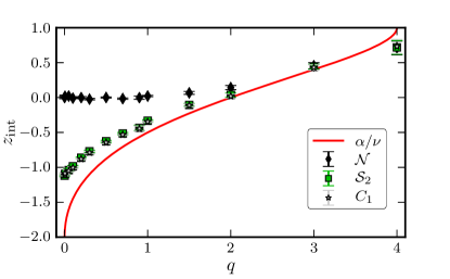
Figure 2: (Color online) Estimates of the 2D dynamical critical exponents $z_{\mathrm{int},{\cal O}}$ for ${\cal O}={\cal N}$, ${\cal S}_{2}$ and $C_{1}$, respectively, as a function of $q$. The line corresponds to the Li-Sokal bound $z_{\mathrm{int}}>\alpha/\nu$ Li and Sokal (1989).

A number of different techniques for the practical estimation of autocorrelation times have been discussed in the literature. We use a direct summation of the autocorrelation function according to Eq. (11). Since, for any time lag, the estimated autocorrelation function adds a constant amount of noise per term, a cutoff $\Lambda$ needs to be introduced to ensure a finite variance of the estimator for the autocorrelation time Priestley (1996). A technique with an adaptive summation window has originally been suggested in Ref. Madras and Sokal (1988). We use a modification of this approach discussed more recently in Ref. Wolff (2006). Determining $\Lambda$ involves a tradeoff between the bias for small cutoffs and the exploding variance as $\Lambda\rightarrow M$. This balance is struck here by numerically minimizing the quantity

$$\exp{\left(-\Lambda/\tau\right)}+2\sqrt{\Lambda/M},$$ (14)

which is proportional to the sum of the relative statistical and systematic errors. We find this procedure to yield stable results throughout. In particular, the estimates of $\tau_{\mathrm{int}}$ are consistent with those found from an alternative jackknifing technique Weigel and Janke (2010); Efron and Tibshirani (1994).

To achieve an appropriate judgment of Sweeny’s algorithm in the different implementations against other approaches of simulating the RCM, we need to combine the information contained in the autocorrelation times with those of the run-times for the different operations involved. We hence compare the effective run-time to create a statistically independent sample of a given observable, where independence is understood in the sense of Eq. (12). To this end, we consider the effective runtime per edge,

$$T_{\mathcal{O}}\equiv\tau_{\mathrm{int},\mathcal{O}}\bar{t},$$ (15)

where $\tau_{\mathrm{int},\mathcal{O}}$ is measured in sweeps and $\bar{t}$ is the runtime per edge operation, averaged over a sufficiently long simulation. Obviously, this quantity is hardware specific, yet by looking at the ratio of two different implementations we expect the specific hardware-dependence to be small .

III.2 Observables and implementation

Figure 3: (Color online) Integrated autocorrelation times as a function of system size for the susceptibility $\mathcal{S}_{2}$ for $q$ ranging from $0.0005$ up to $q=4$. The lines show fits of the functional form (13) to the data.

As $\tau_{\mathrm{int},\mathcal{O}}$ depends on $\mathcal{O}$, any conclusions about the relative efficiency of the Sweeny and Swendsen-Wang-Chayes-Machta dynamics for the RCM might depend on the observable under consideration. It is therefore important to study a number of different quantities covering the energetic and magnetic sectors of the model. For the energetic sector, we studied the number ${\cal N}\equiv b$ of active bonds. In the magnetic sector, we considered the sum of squares of cluster sizes $\mathcal{S}_{2}\equiv\sum_{i=1}^{n}|{\cal C}_{i}|^{2}$, and the size of the largest component $C_{1}\equiv\max_{i=1}^{n}|{\cal C}_{i}|$, where ${\cal C}_{i}$ denotes the $i$th cluster resulting from the set of active bonds. These observables of the RCM are related to standard observables of the Potts model Weigel et al. (2002); Garoni et al. (2011), namely the internal energy per spin $u=\langle\mathcal{N}\rangle/(L^{d}p)$, the susceptibility $\chi=\langle\mathcal{S}_{2}\rangle/L^{d}$, and the order parameter $m=\langle C_{1}\rangle/L^{d}$.

We implemented a code for the Sweeny update using the four variants of connectivity algorithms discussed above in Sec. II, i.e., sequential breadth-first search (SBFS), interleaved BFS (IBFS), union-and-find (UF), as well as dynamic connectivities (DC). Our program was implemented in C and compiled with the GNU Compiler Collection (GCC) 4.5.0 at -O2 optimization level on an Intel Xeon E4530 $2.66$ GHz. The available memory was $16$ GB. These specifications resulted in speed ups through caching effects – mainly for the DC implementation, see the discussion below – for system sizes $L\leq 48$, which approximately corresponds to a memory footprint of the size of the L2 cache of $6$ MB for the DC implementation.

The implementations based on BFS and union-and-find both require memory scaling as $\mathcal{O}(L^{2})$. The DC code, on the other hand, requires to maintain $\mathcal{O}(\log L)$ separate forests, leading to a total memory requirement of $\mathcal{O}(L^{2}\log L)$ Iyer et al. (2001). In practise for a system of size $L=1024$ and $q=2$ at criticality, the BFS and UF implementations required around $10$–$15$ MByte, whereas the DC code used approximately $3.5$ GByte.

The random number stream was generated by a GSL implementation of the Mersenne twister or MT19937 generator Matsumoto and Nishimura (1998) which has a very large period of $2^{19937}\approx 10^{6000}$ and, more importantly, was shown to be equi-distributed in less then $623$ dimensions.

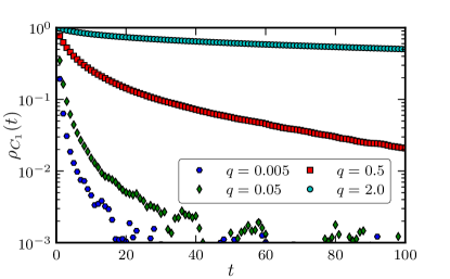
Figure 4: (Color online) Normalized critical autocorrelation function for the order parameter $C_{1}$ and several values of $q$. The linear system size is $L=64$. Time is counted in units of $L$ single bond moves here, such that $L=64$ time steps correspond to a lattice sweep.

III.3 Simulation results

In order to test the predicted asymptotic run-time behavior and determine the dynamic critical behavior of Sweeny’s algorithm, we performed a series of simulations of the RCM on the square lattice. To cover the complete range of systems with continuous phase transitions, we chose $q=0.0005$, $0.005$, $0.05$, $0.1$, $0.2$, $0.3$, $0.5$, $0.7$, $0.9$, $1$, $1.5$, $2$, $3$ and $4$. Simulations were performed for a series of $14$ system sizes ranging from $L=4$ up to $L=1024$. All simulations were done at the exact critical coupling $v_{c}=\sqrt{q}$ Wu (1982). While, typically, observable measurements in Markov chain Monte Carlo are taken after every lattice sweep of updates Binder and Landau (2009), for the case of the bond algorithm and relatively small values of $q$, it turned out that the fast decorrelation leads to autocorrelation times way below a single sweep. To resolve these effects, we hence changed the measurement interval to multiples of $L$, which turned out to be a good compromise between the visibility of correlations and the resulting lengths of time series. This setup resulted in at least $2^{20}$ and up to $2^{23}$ measurements for some system sizes. As a result, our simulations were at least $10^{3}$, and at best $10^{5}$ times the relevant time scale $\tau_{\mathrm{exp}}$. Consistent with Sweeny’s original observation, we were able to equilibrate all runs in less then $200$ sweeps.

III.3.1 Dynamical critical behavior

We first considered the behavior of the energy-like observable ${\cal N}$, determining (integrated) autocorrelation times according to Ref. Wolff (2006) with resulting cutoff parameter $\Lambda_{\cal N}$ (see the discussion in Sec. III.1 above). In order to extract the corresponding dynamical critical exponents we fitted a power-law of the form $\tau_{\mathrm{int}}\sim L^{z_{\mathrm{int}}}$ to the data, omitting some of the smallest system sizes to account for scaling corrections. The quoted errors on fit parameters correspond to an interval of one standard deviation. The resulting estimates of $z_{\mathrm{int},{\cal N}}$ are shown in Fig. 2 and the numerical values are summarized in Table 2. Note that $z_{\mathrm{int},{\cal N}}\approx 0$ for $q\leq 2$. This is in agreement with a key result due to Li and Sokal, providing a lower bound for the autocorrelation times of $\mathcal{N}$ and its corresponding dynamical exponents Li and Sokal (1989); Garoni et al. (2011)

$$\tau_{\mathrm{exp},\mathcal{N}}\gtrsim\tau_{\mathrm{int},\mathcal{N}}\geq C_{v}\;\Rightarrow\;z_{\mathrm{exp},\mathcal{N}}\geq z_{\mathrm{int},\mathcal{N}}\geq\alpha/\nu,$$ (16)

where $C_{v}$ is the specific heat and $\alpha/\nu$ the associated finite-size scaling exponent. While this result was originally derived for the Swendsen-Wang dynamics, it was also shown to hold for the Sweeny algorithm Li and Sokal (1989); Deng et al. (2007a). As $\alpha/\nu\leq 0$ for $q\leq 2$ Wu (1982), our data are consistent with this bound and indicate that it is close to being tight for the Sweeny dynamics on the square lattice for $q\geq 2$, cf. Fig. 2. The values for $q=4$ appear to violate this bound, but we attribute these deviations to the logarithmic corrections expected for this particular value of $q$, preventing us from seeing the truly asymptotic behavior in the regime of system sizes considered here.

We next turned to the magnetic observables ${\cal S}_{2}$ and $C_{1}$. Deng et al. Deng et al. (2007a) first showed that under the Sweeny dynamics the susceptibility ${\cal S}_{2}$ exhibits a surprisingly fast decorrelation on short timescales and, in particular, the corresponding integrated autocorrelation time $\tau_{\mathrm{int},\mathcal{S}_{2}}$ decreases with increasing system size, indicating a negative value of the corresponding dynamical critical exponent $z_{\mathrm{int},\mathcal{S}_{2}}$. This phenomenon of critical speeding up is also clearly seen in our data as is illustrated in the plot of the $L$ dependence of the autocorrelation times of ${\cal S}_{2}$ in Fig. 3. A rather similar behavior is found for the order parameter $C_{1}$. The initial fast decay of correlations is illustrated in Fig. 4, where it is clearly seen that $C_{1}$ is completely decorrelated in less than a single sweep for $q\lesssim 2$. Note that the measurements along the Markov chain are still correlated, but with a system size scaling weaker than $L^{2}$ such that the impression of a complete decorrelation appears on the scale of sweeps.

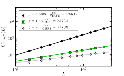
Figure 5: (Color online) Number of vertices $C_{\mathrm{min},2}$ of the smaller of two adjacent clusters as visited in a 2D simulation using IBFS following (preceding) the deletion (insertion) of an external edge. The lines show fits of the power-law form $C_{\mathrm{min},2}=AL^{y_{\textrm{IBFS}}^{(e)}}$ to the data.

The values of $z_{\mathrm{int},\mathcal{S}_{2}}$ resulting from power-law fits to the autocorrelation times are compiled in Table 2. As is clearly seen from the plot of the data in Fig. 3, we find $z_{\mathrm{int},\mathcal{S}_{2}}\leq 0$ for $q\leq 2$. Regarding the dynamical critical exponents in the magnetic sector, we find $z_{\mathrm{int},C_{1}}=z_{\mathrm{int},\mathcal{S}_{2}}$ within our error bars. The authors of Ref. Deng et al. (2007a) suggested to determine $z_{\mathrm{int},\mathcal{S}_{2}}$ from a data collapsing procedure using a two-time scaling ansatz combining the fast initial decay with a slower exponential mode for longer times. In our studies, however, we found this approach to yield rather unstable results and thus chose, instead, to perform more conventional fits to a power law.

We note that, in line with Ref. Garoni et al. (2011) we used the summation cutoff $\Lambda_{\mathcal{N}}$ of the observable $\mathcal{N}$ for all observables, because the magnetic observables ${\cal S}_{2}$ and $C_{1}$ with their fast initial decay would lead to very small, sub-asymptotic cutoffs if the rule of Ref. Wolff (2006) would be directly applied. We also checked that the estimators for $\tau_{\mathrm{int},\mathcal{S}_{2}}$ and $\tau_{\mathrm{int},C_{1}}$ were on a plateau so that a change in the summation window mainly influences the variance of the estimator, which is monotonically increasing with $\Lambda$.

Table 3: Run-time scaling exponents in two dimensions according to Eq. (17) for the SBFS, IBFS and the UF implementation. The scaling exponents $\gamma/\nu$ and $d_{F}-x_{2}$ are shown for reference and comparison. The $y$ exponents correspond to scaling $\sim L^{y}$ of the number of vertices touched in a sequential (SBFS) and interleaved (IBFS) breadth-first cluster traversal for internal (i) and external (e) edges, respectively.

$q$	$\kappa_{\mathrm{SBFS}}$	$\kappa_{\mathrm{IBFS}}$	$\kappa_{\mathrm{UF}}$	$y_{\textrm{IBFS}}^{(i)}$	$y_{\textrm{IBFS}}^{(e)}$	$y_{\textrm{SBFS}}^{(i)}$	$y_{\textrm{SBFS}}^{(e)}$	$d_{F}-x_{2}$	$\gamma/\nu$
0.0005	$1.81(1)$	$1.18(3)$	$1.54(6)$	$1.25(1)$	$1.24(1)$	$1.25(1)$	$1.99(1)$	1.23407	1.99296
0.005	$1.80(2)$	$1.14(2)$	$1.70(6)$	$1.22(1)$	$1.21(1)$	$1.22(1)$	$1.98(1)$	1.20021	1.97823
0.05	$1.74(1)$	$1.02(3)$	$1.77(4)$	$1.10(1)$	$1.11(1)$	$1.11(1)$	$1.93(1)$	1.09783	1.93580
0.1	$1.72(1)$	$0.97(2)$	$1.78(3)$	$1.05(1)$	$1.05(1)$	$1.06(1)$	$1.91(1)$	1.03881	1.91284
0.5	$1.65(2)$	$0.71(3)$	$1.77(2)$	$0.82(1)$	$0.82(1)$	$0.82(1)$	$1.83(1)$	0.80768	1.83449
0.7	$1.63(2)$	$0.69(4)$	$1.77(4)$	$0.75(2)$	$0.76(1)$	$0.76(2)$	$1.81(1)$	0.73541	1.81407
1	$0$	$0$	$1.74(2)$	$0.66(1)$	$0.67(1)$	$0.67(1)$	$1.79(1)$	0.64583	1.79167
1.5	$1.56(2)$	$0.43(2)$	$1.71(3)$	$0.55(2)$	$0.56(1)$	$0.57(2)$	$1.75(1)$	0.52298	1.76644
2	$1.57(2)$	$0.35(3)$	$1.68(3)$	$0.46(2)$	$0.47(2)$	$0.48(3)$	$1.73(1)$	0.41667	1.75000
3	$1.52(4)$	$0.19(1)$	$1.67(2)$	$0.32(3)$	$0.30(4)$	$0.35(3)$	$1.69(2)$	0.21667	1.73333
4	$1.42(4)$	$0.13(2)$	$1.64(7)$	$0.22(11)$	$0.23(1)$	$0.26(1)$	$1.68(1)$	-0.12500	1.75000

Comparing our results for the Sweeny dynamics to the Swendsen-Wang algorithm, we note that, apart from the slightly smaller dynamical critical exponent for the former, we also find somewhat smaller amplitudes in the $\tau_{\mathrm{int}}=AL^{z_{\mathrm{int}}}$ scaling for the bond algorithm. Hence for $L=256$ we find, e.g., $\tau_{\mathrm{int},{\cal S}_{2}}\approx 0.1$ ($q=1$) and $\approx 10$ ($q=3$) for the Sweeny update, while values of $\tau_{\mathrm{int},{\cal S}_{2}}\approx 0.5$ ($q=1$) and $\approx 36$ ($q=3$) are found for the Swendsen-Wang update.

III.3.2 Run-time scaling

As discussed above, the relevant time scales for a comparison of the bond algorithm against other approaches depend on both, the statistical decorrelation as well as the run-time scaling of the elementary operations. We therefore analyzed average run-times for bond updates in the Sweeny algorithm with the different implementations of connectivity updates discussed in Sec. II.2.

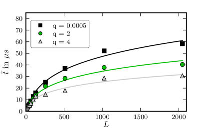
Figure 6: (Color online) Average run-time $\bar{t}$ for several values of $q$ and $L$ for the Sweeny update using a dynamic connectivity (DC) algorithm based on splay trees. The lines correspond to least-squares fits of the model (18) to the data.

For the techniques based on BFS, we studied the number of steps required to complete a connectivity check for the case of operations on internal and external edges, respectively, for the SBFS and SBFS implementations. For internal edges, this corresponds to the number of vertices touched by the BFSs until a re-connecting path is found. For external edges such a path is not found and the search hence terminates after a number of steps corresponding to the mass of either the first cluster (SBFS) or the smaller cluster (IBFS). Checking the number of steps for operations on internal and external edges for SBFS and IBFS, respectively, we used power-law fits according to $\sim L^{y}$ to extract estimates of the four exponents $y_{\textrm{SBFS}}^{(i)}$, $y_{\textrm{SBFS}}^{(e)}$, $y_{\textrm{IBFS}}^{(i)}$, and $y_{\textrm{IBFS}}^{(e)}$. The fit results are collected in Table 3. The data and corresponding fits for the case of the number of steps $C_{2,\mathrm{min}}$ relevant for the operation on an external edge with IBFS are shown in Fig. 5. The exponents $y$ follow the asymptotic values $\gamma/\nu$ and $d_{F}-x_{2}$, respectively, derived above in Sec. II.2.1 and also listed in Table 3 for comparison.

For the total average run-time per bond operation, we asymptotically expect power-law behavior as well,

$$\bar{t}\sim L^{\kappa}.$$ (17)

This assumption in general describes well our data — with only minor deviations for smaller system sizes due to caching effects. For SBFS, we expect the different asymptotic scaling behavior for operations on internal and external edges, respectively, to result in an effective run-time exponent $\kappa$ somewhere in between the exponents $d_{F}-x_{2}$ and $\gamma/\nu$ relevant to operations on internal and external edges, respectively (recall that internal and external edges occur in constant fractions). Our estimates of $\kappa_{\mathrm{SBFS}}$ listed in Table 3 are in line with these expectations. We have no doubt, however, that the asymptotically expected $\kappa_{\mathrm{SBFS}}=\gamma/\nu$ ultimately holds for sufficiently large systems. For the interleaved case, on the other hand, all four operation types exhibit $y=d_{F}-x_{2}$, and we hence find $\kappa_{\mathrm{IBFS}}$ consistent with $d_{F}-x_{2}$ already for the system sizes considered here, cf. Table 3.

The analysis of the run-time behavior for the union-and-find approach is more subtle as the insertion of edges is performed in constant time, whereas the deletion of edges incurs an effort proportional to $L^{d_{F}-x_{2}}$ and $L^{\gamma/\nu}$ for internal and external edges, respectively, cf. Table 1. As a consequence of the different scaling of individual operations, the effective run-time scaling exponent $\kappa_{\mathrm{UF}}$ according to Eq. (17) is again found to be smaller than the expected limiting value $\gamma/\nu$, see the values compiled in Table 3.

The scaling of run-times per step for our implementation of the dynamic connectivity algorithm and a representative selection of $q$-values is shown in Fig. 6. We find a sub-algebraic growth and, according to the asymptotic run-time bounds derived in Ref. Holm et al. (2001), we fitted the functional form

$$\bar{t}(L)=a\log^{2}L+b\log L+c$$ (18)

to the data. The fits resulted in $c\approx 0$ such that we fixed $c=0$ in the following. Somewhat surprisingly, our fits yield $b<0$; we interpret this as a result of the presence of correction terms and the amortized nature of the run-time bounds leading to the asymptotic scaling only being visible for very large system sizes. Similar observations have been reported for general sets of inputs in Ref. Iyer et al. (2001). Considering the ratio $a/b$, we find that its modulus increases with $q$, yielding a value of $\approx 0.3$ for $q=0.0005$ and $\approx 0.71$ for $q=2$. This corresponds to the increasing fraction of non-tree edges for increasing $q$, resulting in an increase of traversals of the edge level hierarchy with the associated ${\cal O}(\log^{2}L)$ complexity. Irrespective of that, as a consequence of the larger number of cluster-splitting operations the total run-time is found to be largest for small $q$, cf. Fig. 6.

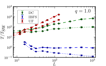
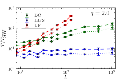
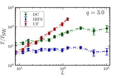
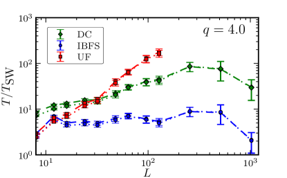
Figure 7: (Color online) Effective run-times $T$ according to Eq. (15) for the different implementations relative to the time $T_{\mathrm{SW}}$ of the Swendsen-Wang algorithm Swendsen and Wang (1987). Dashed lines correspond to the run-time to generate an independent sample of the observable $\mathcal{N}$ and dotted lines to samples of $\mathcal{S}_{2}$.

We also investigated the effect of the unconditional acceptance of proposed updates for the Metropolis rule as discussed in Sec. II.1 above. This adds another $q$ dependent, but system-size independent, element to the run-time scaling. Such unconditional moves can save significant computational effort in case no data structures have to be updated after move acceptance. This is the case for the algorithms based on BFS which are “stateless” in the sense that no explicit record of connectivity is kept. Unconditional insertion or removal of edges in this case does not entail any further computational effort. On the contrary, unconditional insertion or removal lead to data-structure updates for the union-and-find and DC implementations. As a consequence, we find a constant speed-up for the BFS based implementations proportional to $1/[1-\min(\sqrt{q},1/\sqrt{q})]$. In the singular case $q=1$, BFS performs all edge updates in constant time as all insertions and deletions can be performed unconditionally such that no cluster traversals are necessary. On the contrary, no performance improvement from unconditional moves is observed for the more elaborate UF and DC implementations.

We note that, for all implementations, the average run-time per bond operation depends quite strongly on $q$. This is, on the one hand, due to the $q$ dependence of the fraction $r_{\mathrm{ext}}$ of external edges reaching from $r_{\mathrm{ext}}=1$ for $q\to 0$ down to $r_{\mathrm{ext}}=0.33$ for $q=4$. For the case of the BFS implementations, an additional $q$ dependence is introduced through the unconditional moves as discussed above.

III.3.3 Overall efficiency

As discussed above in Sec. III.1, the relevant measure for the overall efficiency of various implementations of cluster algorithms is the total run-time for the generation of a statistically independent sample according to Eq. (15). We compared the effective run-times of all three implementations of the bond algorithm with a reference code for the Swendsen-Wang dynamics. As the dynamical critical exponents $z_{\mathrm{int}}$ for the Sweeny update are found to be smaller than those of the Swendsen-Wang-Chayes-Machta dynamics, see Refs. Deng et al. (2007a, b); Garoni et al. (2011) and Table 2, we can expect asymptotically more efficient simulations for cases where the run-time exponent $\kappa<z_{\mathrm{int},{\cal O}}^{\mathrm{SW}}-z_{\mathrm{int},{\cal O}}$. Since any poly-logarithm is dominated by $L^{\epsilon}$ with $\epsilon>0$, this is clearly the case, asymptotically, for the DC algorithm. From the data for $z_{\mathrm{int},{\cal O}}^{\mathrm{SW}}-z_{\mathrm{int},{\cal O}}$ in Table 2 and those for $\kappa$ in Table 3, it is seen that for $1<q\leq 4$, this condition is not met for the implementation based on union-and-find. For the technique based on (interleaved) breadth-first-search, on the other hand, such a case arises (for integer values $q$) only for $q=4$, where $z_{\mathrm{int},{\cal O}}^{\mathrm{SW}}-z_{\mathrm{int},{\cal O}}\approx 0.16$ and $\kappa_{\mathrm{IBFS}}=0.13(2)$. These observations are corroborated by the plots of the relative efficiencies shown in Fig. 7. For comparison, we here show the results for the two observables ${\cal N}$ and ${\cal S}_{2}$ with significantly different behavior for $q\leq 2$. From the plots for the integer values $q=2$, $3$ and $4$, it is clear that in absolute run-times IBFS is most efficient for the range of system sizes $L\leq 1024$ considered here. Hence, the asymptotic advantage of the DC algorithm only shows for system sizes beyond this range. The downturn of the ratio $T/T_{\mathrm{SW}}$ for the largest system sizes and $q=4$ observed for the BFS and DC codes might be an indication of the asymptotic run-time advantage of Sweeny’s algorithm over Swendsen-Wang with these connectivity algorithms as discussed above. The results for the percolation case $q=1$ using IBFS, on the other hand, are of exceptional nature as there the cost of bond operations is completely independent of system size due to the effect of unconditional acceptance. For the case of ${\cal S}_{2}$, one even finds a decrease of the relative cost of generating a statistically independent sample as this observable profits from the initial fast decorrelation or critical speeding up.

For the most relevant case $q\leq 1$, where Sweeny’s algorithm provides the only means of simulation, we cannot compare to another algorithm. Instead, we present in Fig. 8 a comparison of run times for the SBFS, IBFS, UF and DC implementations for $q=0.005$. As here $\kappa_{\mathrm{IBFS}}$ is relatively unfavorable, we observe a clear advantage for the DC algorithm which is significantly more efficient than the other options in the full range of studied system sizes $4\leq L\leq 1024$. UF is found to be even less efficient than SBFS here which might be considered surprising in view of the fact that all insertions are performed at constant cost and deletions have the same asymptotic run-time bounds as SBFS, see Table 1. This is easily understood, however, noting that the factor of two gained for UF from the 50% of operations performed in constant time is spent again in having to traverse both clusters fully in case of external edge deletions. Taking into account overheads for data-structure updates for UF, this explains the slight disadvantage of UF over SBFS seen in Fig. 8.

IV Conclusions

We have shown that it is possible to implement Sweeny’s algorithm efficiently and in a lattice and dimensionality independent way, using a dynamic connectivity (DC) algorithm, in the sense that the runtime dependence on the system size is poly-logarithmic and only contributes a correction to the statistical $L^{z_{\mathrm{int}}}$ contribution of the runtime to create an effectively uncorrelated sample. Compared to the Swendsen-Wang-Chayes-Machta algorithm, we also find somewhat smaller dynamical critical exponents, leading to an overall asymptotically more efficient simulation of the random-cluster or Potts model with Sweeny’s approach. In addition, the bond algorithm is the only known approach for simulations in the regime $q<1$ including, for instance, interesting $q\rightarrow 0$ limits such as the maximally connected spanning sub-graphs of Ref. Jacobsen et al. (2005).

Figure 8: (Color online) Run-time per edge operation of simulations of the $q=0.005$ square-lattice RCM and the bond algorithm employing the SBFS, IBFS, UF and DC connectivity implementations, respectively.

We analyze in detail four implementations based on (sequential and interleaved) breadth-first searches, on union-and-find data structures, and on the fully dynamic connectivity algorithm suggested in Ref. Holm et al. (2001), respectively. For each implementation, we derive average run-time bounds for insertions and deletions of internal and external edges, respectively, and deduce the overall asymptotic run-time behavior. It is found that interleaved breadth-first searches, although relatively unfavorable as compared to union-and-find and dynamic connectivities at first sight, perform rather well due to the lack of an underlying data structure encoding the connectivity of the clusters, in particular if connectivity queries are omitted whenever possible due to accepting moves for which the drawn random number indicates acceptance irrespective of the result of the connectivity query. The union-and-find based implementation, on the other hand, although superior in asymptotic run-time in three out of four cases of insertions or deletions of internal or external edges, shows ultimately inferior performance due to the run-time scaling for deletions of external edges that require full traversals of the involved clusters. The dynamic connectivity algorithm, while asymptotically most efficient with a poly-logarithmic scaling of run-times per operation, has rather large constants leading to somewhat weaker performance than breadth-first search for the considered lattice sizes $L\leq 1024$ and $q\geq 1$. For $q\ll 1$, on the other hand, where run-times are dominated by operations on external edges, it outperforms the other implementations already for small systems. We see significant room for further run-time improvements for the dynamic connectivity algorithm, however, for instance by optimizations of the underlying tree data structure or the implementation of additional heuristics as indicated in the comparative study Iyer et al. (2001). We note that due to the lack of explicit connectivity information for the breadth-first search approach it becomes more expensive than for the other techniques to perform measurements of quantities such as cluster numbers or correlation functions depending on the connectivity. As measurements are typically taken at most once per sweep, however, any cost of at most $L^{2}$ operations for measurements results in only ${\cal O}(1)$ amortized effort per bond operation.

The observed fast initial decorrelation for $q\leq 2$ and quantities such as ${\cal S}_{2}$ and $C_{1}$ depending on cluster connectivity as illustrated in Figs. 2, 3 and 4 suggests that there is an additional dynamical mechanism at play for such observables. As argued in Ref. Deng et al. (2007a), this is due to a larger number of operations on external edges for smaller values of $q$ which can lead to a large-scale change in the connectivity structure through a single bond operation. The concentration of external edges, bridges or fragmenting bonds drastically increases as $q$ is decreased from $4$ down to the tree limit $q\to 0$ Elçi and Weigel which is also clearly expressed in a corresponding increase in the fractal dimension of “red” bonds Stanley (1977). It is currently not clear, however, why this effect only leads to a change in dynamical critical behavior for $q\leq 2$.

While we have restricted our attention to simulations on the square lattice, all implementations discussed here are essentially independent of the underlying graph or lattice, requiring only minimal adaptations for different situations. This makes our approach significantly more general than the implementation originally suggested by Sweeny Sweeny (1983) which is based on tracing loops on the medial lattice in two dimensions. Additionally, the latter technique in two dimensions still suffers from polynomial scaling of the run-time per edge operation Deng et al. (2010), such that a poly-logarithmic implementation is asymptotically faster.

Until now we have only used the DC implementation for canonical simulations but as proposed in Ref. Weigel (2010) an interesting application are generalized-ensemble simulations of the random cluster model where one directly estimates the number of possible graphs $g(k,b)$ with $k$ clusters and $b$ edges which then allows for the calculation of canonical ensemble averages as continuous functions of temperature and the parameter $q$.

The source code of the implementations discussed here, in particular including the dynamic connectivity algorithm, is available on GitHub under a permissive license swe .