Supplementary Materials:
Corruption Drives the Emergence of Civil Society

1 Calculation of Stationary Distribution

Our model of cooperation follows the common formulation of evolutionary dynamics simulations [novakBook]. Specifically we consider a set of $M$ agents each subscribing to one of $d$ strategies. At each time step a random sample of $N$ agents are chosen to play a public goods game. The payoffs received by each agent are determined by the number of each type of strategy. At each time step 2 agents are randomly chosen and their payoffs are compared. The probability of one agent imitating the other is determined by a logistic function of the difference in payoffs and an imitation strength $s$. There is also a small probability $\mu$ that a randomly chosen agent will undergo a mutation to a different strategy.

In order to calculate the stationary distribution of strategies in our evolutionary dynamics we consider, in common with previous work on life-death processes [fudenberg], the rates of transitions between homogeneous states in which all agents subscribe to a single strategy. Under deterministic dynamics these homogeneous states may be absorbing i.e. Once cooperation has collapsed and defectors have taken over, the system cannot return to a homogeneous state of cooperators. However random mutation allows mixing between homogeneous states via mutation and subsequent fixation.

Consider a population of agents each subscribing to strategy $X$. The probability that the system makes the transition to the state of all agents subscribing to a different strategy $Y$ depends on the product of two quantities;

1. The probability that a random mutation introduces an agent with strategy $Y$ ($\mu_{X,Y}$)

2. The probability that this single mutant can invade the population and lead all agents to switch to strategy $Y$; this is known as the fixation probability ($\rho_{X,Y}$).

In this formulation we assume that the mutation rate is low so that each mutation event leads either to fixation of a new homogeneous state or reversion to the same homogeneous state before the next mutation event occurs. Therefore, at any given time, at most two strategies are present.

Addressing (1), mutations occur in the population at a rate $\mu$. The resultant strategy is chosen from the $d-1$ other strategies at random, giving a mutation probability

$$\mu_{X,Y}=\frac{\mu}{(d-1)}$$ (1)

Addressing (2), the fixation probability can be expressed explicitly from the product of the probability of each agent, after the first mutant agent, successively imitating the invading strategy. This requires a detailed description of the payoffs and imitation probabilities (section 1.2). Alternatively, (2) can be inferred simply in the limit of strong imitation (section 1.1).

Once we have an expression for the transition matrix between the homogeneous states, we can find the stationary distribution of the system of agents as the dominant eigenvector. This is a vector of values of size $d$ which represents the long run probabilities of finding the system in a given state. We require that the transition matrix $T$ be row normalised i.e. If the system is found in state $X$ it must either remain in state $X$ or transition to state $k\neq X$. Because the stationary distribution tells us the relative proportions of each state and the fact that the mutation probability does not depend on the source or target states, the actual numerical value of $\mu$ is not important and it is convenient to omit it from $T$.

For a simple system of $d=$ 3 states $X$,$Y$ and $Z$ representing cooperators, defectors and non-participants respectively, we can construct $T$

$$T=\begin{pmatrix}1-\frac{1}{2}\rho_{X,Y}-\frac{1}{2}\rho_{X,Z}&\frac{1}{2}\rho_{X,Y}&\frac{1}{2}\rho_{X,Z}\\ \frac{1}{2}\rho_{Y,X}&1-\frac{1}{2}\rho_{Y,X}-\frac{1}{2}\rho_{Y,Z}&\frac{1}{2}\rho_{Y,Z}\\ \frac{1}{2}\rho_{Z,X}&\frac{1}{2}\rho_{Z,Y}&1-\frac{1}{2}\rho_{Z,X}-\frac{1}{2}\rho_{Z,Y}\\ \end{pmatrix}$$ (2)

The factor of $\frac{1}{2}$ corresponds to $\frac{1}{d-1}$.

1.1 Strong Imitation Limit

The individual entries of $T$ can be populated by simple arguments under the limit $s\rightarrow\infty$ (and under suitable conditions for other parameters such as punishment strength or cost) so that a strategy with a superior payoff will always be imitated and an inferior payoff will not. There are in fact only 3 possible values for the fixation probabilities $\rho_{i,j}$

1. If $P_{j}<P_{i}$ for a single mutant with strategy $j$, then the mutation cannot invade and the fixation probability is 0.

2. If $P_{j}>P_{i}$ for a single mutant with strategy $j$, then the mutation is beneficial and induces transition to a homegenous state $j$

3. This is peculiar to a single cooperator attempting to invade non-participants. The non-participants receive a fixed payoff of $\sigma$ but a single cooperator will also receive a payoff $\sigma$ since she has no partner with which to participate in a PGG. At the next imitation event involving the mutant cooperator, the cooperator will have the opportunity to imitate a non-participant. Since the payoffs are identical, the cooperator will revert to a non-participant with probability $\frac{1}{2}$, but is equally likely to convert a non-participant to cooperation under a neutral drift. Once two or more cooperators are present, this strategy is dominant and they invade with probability 1.

Our intuitive understanding of PGGs tells us that in the absence of punishment, free-riding always pays ($\rho_{X,Y}=1$) and that unilateral cooperation in the face of defection does not ($\rho_{Y,X}=0$). When cooperation is underway, it pays to participate ($\rho_{X,Z}=0$) and due to the argument above, cooperators are slow to take over non-participants ($\rho_{Z,X}=\frac{1}{2}$). Finally, if no-one is playing the PGG then something is better than nothing ($\rho_{Y,Z}=1$ and $\rho_{Z,Y}=0$). Therefore $T$ reduces to

$${T=\begin{pmatrix}\frac{1}{2}&\frac{1}{2}&0\\ 0&\frac{1}{2}&\frac{1}{2}\\ \frac{1}{4}&0&\frac{3}{4}\\ \end{pmatrix}}$$ (3)

Leading to a stationary probability $\left[\frac{1}{4},\frac{1}{4},\frac{1}{2}\right]$; the systems spends half of its time in a state of non-participation and an equal one quarter both as all cooperators or defectors. Intuitively there is a single cycle from full cooperation, which may only be invaded by defectors (under the assumption that $\sigma<\frac{Ncr}{N-1}$). Defectors in turn may only be invaded by non-participants. Once in a state of full non-participation, the population may only slowly be invaded by cooperators due to the argument above leading to a fixation probability of $\frac{1}{2}$. Therefore non-participation predominates over long time averages as seen in simulation.

1.2 Explicit Calculation of Transition Probabilities (Intermediate Imitation Strength)

The dynamics of the evolution of cooperation amongst a finite-sized population of agents diverges from the behaviour of mean-field treatments such as replicator dynamics. Now the stochastic effects of mutation become significant [traulsen]. The fixation probability of an $l$ mutant in an otherwise homogeneous population of $k$ agents, (2), can be calculated explicitly from the theory of birth-death processes [novakBook] as

$$\rho_{k,l}=\frac{1}{1+\sum_{q=1}^{M-1}\Pi_{N_{l}=1}^{q}\frac{\tau_{l\rightarrow k(N_{l})}}{\tau_{k\rightarrow l(N_{l})}}}$$ (4)

Where $M$ is the size of the population and the number of agents with strategy $k$ or $l$ respectively is given by $N_{k}$ and $N_{l}$ with $M=N_{k}+N_{l}$. Here $\tau_{l\rightarrow k(N_{l})}$ represents the probability that one of the $N_{k}$ players will convert to strategy $l$ via imitation. This transition probability for a single agent can be written explicitly for a Moran process obeying a logistic imitation probability.

$$\tau_{l\rightarrow k}(N_{l})=\frac{N_{l}}{M}\frac{M-N_{l}}{M}\frac{1}{1+\exp{[-s(P_{k}-P_{l})]}}$$ (5)

Where $s$ is the imitation strength and $P_{k}$ and $P_{l}$ are the payoffs of strategies $k$ and $l$ which depend on the number of $k$ and $l$ players. Thankfully the fixation probability simplifies to

$$\rho_{k,l}=\frac{1}{1+\sum_{q=1}^{M-1}\exp[-s\sum_{N_{l}=1}^{q}(P_{k}-P_{l})]}$$ (6)

Although there is no analytical expression for this at intermediate values of $s$, the sums can be readily evaluated and the entries of $T$ calculated. In turn the stationary distribution can be calculated.

Henceforth, unless otherwise specified, we use the following parameter values.

PGG contribution	c	1.0
PGG multiplier	r	3.0
Population size	M	100
Sample size	N	5
Imitation strength	s	1000
Non-participation payoff	$\sigma$	0.1
Pool punishment effect	B	0.7
Pool punishment cost	G	0.7
Peer punishment effect	$\beta$	0.7
Peer punishment cost	$\gamma$	0.7
Bribe as proportion of tax	K	0.5

2 Replicating Results of Sigmund et al

Sigmund et al [sigmund] calculate the stationary distributions of their simulations in an analagous way. However the introduction of new punishing strategies introduces a fourth possible value for the fixation probability. When a peer-punishing mutant arises in a homogeneous population of cooperators, there is neutral drift since peer-punishers have no-one to punish so enjoy the same benefits as cooperators with no additional costs. This leads to a fixation probability of $\frac{1}{M}$ [novakBook]. In this scheme, the possible strategies are:

Cooperators ($X$):

Participate and contribute $c$ to the PGG

Defectors ($Y$):

Participate but do not contribute to the PGG

Loners ($Z$):

Neither participate nor contribute to PGG

Peer Punishers ($W$):

Participate and contribute to the PGG (cooperate) and pay a fixed cost per defector $\gamma$ to punish defectors if encountered (the more the defectors, the more the cost).

Pool Punishers ($V$):

Participate and contribute to the PGG (cooperate) and pay a fixed a prior cost $G$ toward a punishment pool (central authority), which will punish defectors if defectors appear.

The payoff is determined by choosing a sample population of size $N$ to play the public good game. Below is the payoff calculations for the different strategies. It is important to point out the second order punishment term $B\times V\times\frac{N-1}{M-1}$, where $B$ is a constant that determines the severity of second order punishment.

$$P_{\sigma} = \frac{\binom{Z}{N-1}}{\binom{M-1}{N-1}}$$

$$P_{second} = \frac{\binom{M-Y-2}{N-2}}{\binom{M-2}{N-2}}$$

$$Y\textrm{ payoff} = (P_{\sigma}.\sigma)+(1-P_{\sigma}).r.c.\frac{M-Z-Y-C}{M-Z}-B(N-1)\frac{V+H}{M-1}-\beta.\frac{(N-1).W+H}{M-1}$$

$$X\textrm{ payoff} = (P_{\sigma}\sigma)+(1-P_{\sigma}).c.\left(r.\frac{M-Z-Y-C}{M-Z}-1\right)-B(N-1)\frac{V+H}{M-1}$$

$$-\beta.\frac{(N-1).W}{M-1}.(1-P_{second})$$

$$Z\textrm{ payoff} = \sigma$$

$$W\textrm{ payoff} = (P_{\sigma}\sigma)+(1-P_{\sigma}).c.\left(r.\frac{M-Z-Y-C}{M-Z}-1\right)-(N-1).\frac{Y+C}{M-1}.\gamma$$

$$-\frac{(N-1)X}{M-1}.\gamma.(1-P_{second})-B(N-1)\frac{V+H}{M-1}$$

$$V\textrm{ payoff} = (P_{\sigma}\sigma)+(1-P_{\sigma}).\left(c.\left[r.\frac{M-Z-Y-C}{M-Z}-1\right]-G\right)$$

The transition matrix is given by:

$$\bordermatrix{&X&Y&Z&V&W\cr X&T_{XX}&T_{XY}&T_{XZ}&T_{XV}&T_{XW}\cr Y&T_{YX}&T_{YY}&T_{YZ}&T_{YV}&T_{YW}\cr Z&T_{ZX}&T_{ZY}&T_{ZZ}&T_{ZV}&T_{ZW}\cr V&T_{VX}&T_{VY}&T_{VZ}&T_{VV}&T_{VW}\cr W&T_{WX}&T_{WY}&T_{WZ}&T_{WV}&T_{WW}\cr}$$ (7)

Where

$$T_{ij}\begin{cases}\frac{1}{4}\mu\rho_{ij}&\text{if }i\neq j\\ 1-\frac{1}{4}\mu\sum_{k\neq i}\rho_{ik}&\text{if }i=j\end{cases}$$ (8)

This reduces to

$$\bordermatrix{&X&Y&Z&V&W\cr X&\frac{3}{4}-\frac{1}{4M}&\frac{1}{4}&0&0&\frac{1}{4M}\cr Y&0&\frac{3}{4}&\frac{1}{4}&0&0\cr Z&\frac{1}{8}&0&\frac{5}{8}&\frac{1}{8}&\frac{1}{8}\cr V&\frac{1}{4}&0&0&\frac{1}{2}&\frac{1}{4}\cr W&\frac{1}{4M}&0&0&0&1-\frac{1}{4M}\cr}$$ (9)

With the stationary distribution $\frac{1}{3M+23}\left[6,6,4,1,3M+6\right]$ i.e. Peer-punishers predominate. See Fig(1).

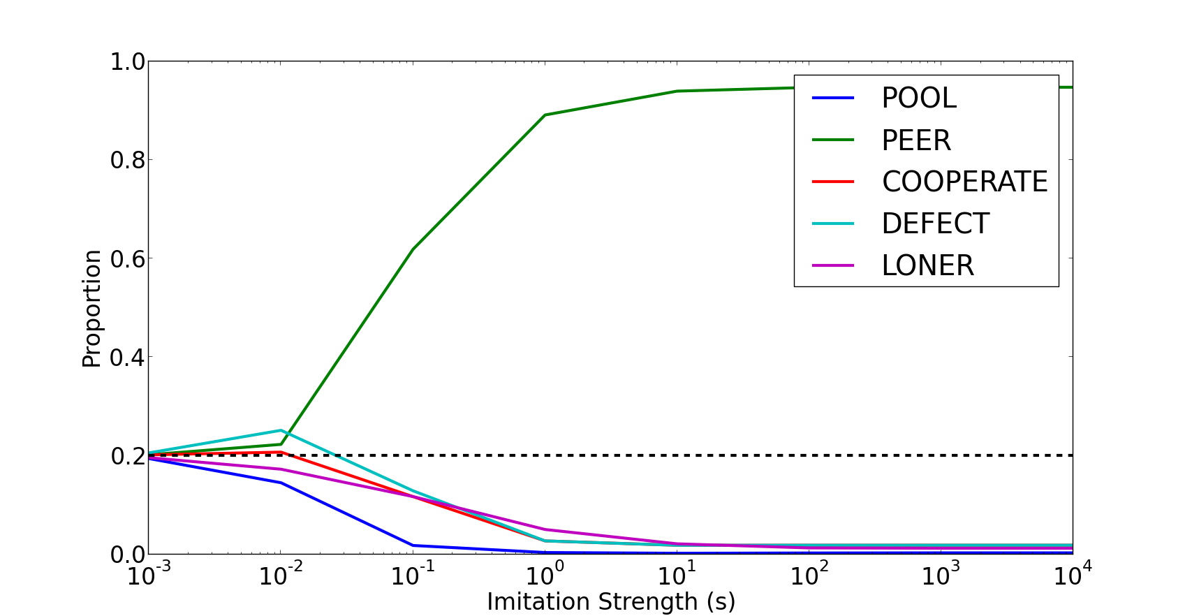
Figure 1: Stationary distributions of states as a function of imitation strength. The dashed line represents equal distribution between the $d$ states.

Including second order punishment leads to pool punishers dominating. Pool punishers now punish defectors, cooperators and peer punishers for not contributing to the pool. Peer-punishers continue to punish defectors and cooperators.

The main differences introduced is that there is no longer a neutral drift between cooperators and peer punishers ($\rho_{X,W}\rightarrow 0$), cooperators no longer invade pool-punishers ($\rho_{V,X}\rightarrow 0$) or peer-punishers ($\rho_{V,W}\rightarrow 0$).

The transition matrix becomes

$$\begin{array}{cccccc}& X& Y& Z& V& W\\ X& \frac{3}{4}& \frac{1}{4}& 0& 0& 0\\ Y& 0& \frac{3}{4}& \frac{1}{4}& 0& 0\\ Z& \frac{1}{8}& 0& \frac{5}{8}& \frac{1}{8}& \frac{1}{8}\\ V& 0& 0& 0& 1& 0\\ W& \frac{1}{4M}& 0& 0& 0& 1-\frac{1}{4M}\end{array}$$ (10)