Population splitting, trapping, and non-ergodicity in heterogeneous diffusion processes

Abstract

We consider diffusion processes with a spatially varying diffusivity giving rise to anomalous diffusion. Such heterogeneous diffusion processes are analysed for the cases of exponential, power-law, and logarithmic dependencies of the diffusion coefficient on the particle position. Combining analytical approaches with stochastic simulations, we show that the functional form of the space-dependent diffusion coefficient and the initial conditions of the diffusing particles are vital for their statistical and ergodic properties. In all three cases a weak ergodicity breaking between the time and ensemble averaged mean squared displacements is observed. We also demonstrate a population splitting of the time averaged traces into fast and slow diffusers for the case of exponential variation of the diffusivity as well as a particle trapping in the case of the logarithmic diffusivity. Our analysis is complemented by the quantitative study of the space coverage, the diffusive spreading of the probability density, as well as the survival probability.

I Introduction

Anomalous diffusion of the power-law form bouchaud ; report

$$\left<x^{2}(t)\right>\sim t^{\beta}$$ (1)

of the mean squared displacement (MSD) has been observed in a wide variety of systems. Depending on the value of the anomalous diffusion exponent $\beta$ we distinguish subdiffusion ($0<\beta<1$) and superdiffusion ($\beta>1$). The special cases are that of normal Brownian motion ($\beta=1$) and wave-like, ballistic motion ($\beta=2$).

Examples for subdiffusion include the anomalous motion of charge carriers in amorphous semiconductors scher , the motion of tracer beads in polymer melts amblard and actin networks weitz , the dynamics of sticky particles along a surface chaikin , or the spreading of tracer chemicals in subsurface hydrology harvey . Superdiffusion is observed in weakly chaotic systems swinney , in bulk-surface exchange controlled dynamics in porous glasses stapf , or for the motion of tracer beads in wormlike micellar solutions ott .

In particular, numerous cases of anomalous diffusion have been reported for the motion of endogenous and artificial submicron tracers in living biological cells, following substantial advances in single particle tracking and spectroscopic tools over the last decade or so pt ; saxton ; franosch13 ; bress13 . Thus, methods such as video tracking, tracking by optical tweezers, or fluorescence correlation spectroscopy have become routine tools to explore the motion of tracers such as larger biomolecules or microbeads in vivo. The anomalous diffusion of submicron-sized tracers is of interest for the understanding of biochemical processes in the cell, but also offers insight into the mechanical properties of the intracellular fluid and cellular mechanical structures as the passive or active tracer motion represents the basis for microrheology micro .

Examples for in vivo subdiffusion include the motion of endogenous granules (lipids or insulin) lene ; tabei ; taylor , of fluorescently labelled RNA molecules golding ; weber , of the tips (telomeres) of eukaryotic DNA and loci of bacterial DNA bronstein ; weber , microbeads guigas ; caspi , viruses seisen01 ; brauchle02 , pigment organelles bruno09 , or of small proteins fradin05 . Potassium channels resident in the plasma membranes of living cells were shown to subdiffuse weigel , as well as the motion of membrane proteins in the Golgi membrane weiss03 . In simulations, subdiffusion of lipid and protein molecules in bilayers and monolayers was observed jeon-lipids ; kneller ; akimoto . Superdiffusion in living cells is observed for motor-driven transport of viruses seisen01 , microbeads caspi , as well as magnetic endosomes robert .

These experimental observations of anomalous diffusion have been modelled theoretically in terms of different generalised stochastic processes pt ; igor ; pccp ; goychuk ; saxton ; franosch13 ; bress13 . The most popular models include obstructed (coralled) diffusion saxton that leads to a turnover between free diffusion and a thermal plateau value. Transiently, this process can be fitted with the law (1). Continuous time random walks scher ; montroll are based on random walk processes, in which the pausing time between successive jumps is power-law distributed such that no characteristic time scale exists, leading to anomalous diffusion of the form (1). In an external potential or in the presence of non-trivial boundary conditions this continuous time random walk process is conveniently described in terms of the fractional Fokker-Planck equation report ; ffpe . The resulting motion of subdiffusive continuous time random walks in intrinsically noisy environments was recently studied nctrw . Fractional Brownian motion mandelbrot and the closely related fractional Langevin equation lutz are driven by Gaussian noise, which is long-ranged correlated in time, again leading to behaviour (1). In the subdiffusive regime these two correlated Gaussian processes are intimately connected with a viscoelastic environment goychuk ; weiss . Some of their properties are shared with scaled Brownian motion fulinski . The law (1) is also effected by the geometrical constraints imposed to a particle diffusing on a support with a fractal dimension havlin ; klemm . Superdiffusion is modelled in terms of fractional Brownian motion or Lévy walks wong ; zukla ; lw1 ; aljaz , a class of continuous time random walks with spatiotemporal coupling.

Above theoretical approaches are based on the assumption that the environment is homogeneous and isotropic, or that over the relevant time and length scales of the measurement spatial variations of the environment in some sense are averaged out. Yet there are clear indications that in biological cells the environment effects strong variations of the local diffusion constant. Thus, maps of the local cytoplasmic diffusion coefficient in bacterial elfDX11 and eukaryotic langDX11 cells indeed demonstrate substantial spatial variations. Significant changes of the diffusivity along the trajectory of single tracer particles in cells may also be affected by transient binding as well as the abundance of biochemical energy supply and transcription activity in different compartments of eukaryotic nuclei platani .

Descriptions in terms of space-dependent diffusion coefficients $D(x)$ are in fact widely used in hydrological applications to mesoscopically describe diffusion in heterogenous porous media hagger95 . In particular, inhomogeneous versions of continuous time random walk models for water permeation in porous ground layers were developed recently hdp-ctrw .

Mathematically, spatially and temporally varying diffusivities give rise to anomalous sub- and superdiffusion in a range of stochastic models, compare Refs. srokowski06 ; srokowski08 ; silva11 ; fulinski ; chechkin-inhom . In particular, Richardson type diffusion in turbulent media was modelled in terms of heterogeneous diffusion processes (HDPs) maglom . Power-law forms for $D(x)$ were proposed to capture the diffusion of a particle on a fractal support fractals-proc , yet, as shown below, this approach gives rise to weakly non-ergodic motion and is inherently different from the ergodic motion on fractals igor ; yazmin . The weakly non-ergodic properties of HDPs were studied recently fulinski ; hdp13 .

Here we analyse in detail the motion of a diffusing particle subjected to a space-dependent diffusion coefficient $D(x)$, for the cases of exponential, power-law, and logarithmic $x$-dependencies. We demonstrate that these processes effect anomalous diffusion of the form (1) of both sub- and superdiffusive forms as well as an ultraslow, logarithmic time dependence. Moreover, we show that despite their description in terms of a time local diffusion equation, these processes exhibit a weak ergodicity breaking in the sense that the time and ensemble averaged MSD do not converge, even in the long time limit, see below. Our study reveals that the dynamics of the diffusing particle may crucially depend on its initial position, and that the time averaged MSD may exhibit a splitting of the entire population of diffusing particles into faster and slower fractions.

In the following Section we briefly review the properties of weak ergodicity violation of stochastic processes. Section III introduces the HDP process in detail. In Sections IV to VI we investigate the power-law, exponential, and logarithmic dependence of $D(x)$. Finally, in Section VII we draw our conclusions and present a brief outlook.

II Weak ergodicity breaking

Commonly we characterise a stochastic process in terms of the ensemble averaged MSD (1) defined through the spatial average of $x^{2}$,

$$\langle x^{2}(t)\rangle=\int x^{2}P(x,t)dx,$$ (2)

over the probability density function (PDF) $P(x,t)$ to find the particle at position $x$ at time $t$. An alternative way to calculate the MSD is via the time average

$$\overline{\delta^{2}(\Delta)}=\frac{1}{T-\Delta}\int_{0}^{T-\Delta}\Big{(}x(t+\Delta)-x(t)\Big{)}^{2}dt$$ (3)

over the time series $x(t)$, whose length is $T$. In the time averaged MSD $\overline{\delta^{2}(\Delta)}$ the differences of the particle positions as separated by the lag time $\Delta$ are evaluated along the trajectory $x(t)$. For a Brownian process, it can be shown that in the limit of long $T$ both definitions of the MSD agree, $\langle x^{2}(\Delta)\rangle=\overline{\delta^{2}(\Delta)}$ pt ; pccp , a manifestation of ergodicity in the Boltzmann sense. Even when $T$ remains finite, a similar equivalence is obtained between the ensemble averaged MSD (1) and the time averaged MSD $\overline{\delta^{2}(\Delta)}$, once we additionally average over a sufficiently large number of individual trajectories pt ; pccp ,

$$\left<\overline{\delta^{2}(\Delta)}\right>=\frac{1}{N}\sum_{i=1}^{N}\overline{\delta_{i}^{2}(\Delta)}.$$ (4)

Once the process is non-stationary, the integral kernel $[x(t+\Delta)-x(t)]^{2}$ will depend on both $\Delta$ and $t$, and the equivalence between ensemble and time averaged MSDs will break down, a phenomenon called weak ergodicity breaking web . In particular, subdiffusive continuous time random walk processes exhibit the linear lag time dependence $\langle\overline{\delta^{2}(\Delta)}\rangle\simeq\Delta$, contrasting the power-law form (1) of the corresponding ensemble average he ; pt ; pccp ; ariel . Under confinement, $\langle x^{2}(t)\rangle$ converges to a plateau, whose value is defined in terms of the second moment of the corresponding Boltzmann distribution, while the time average scales with $\Delta$ as $\overline{\delta^{2}(\Delta)}\simeq\Delta^{1-\beta}$ pt ; pccp ; pnas . Concurrently, subdiffusive continuous time random walk processes age in the sense that physical observables described by this process explicitly depend on the time separation between initial system preparation and start of the measurement johannes . The linear scaling of the time averaged MSD is also observed for correlated vincent and ageing lomholt continuous time random walks, while their respective ensemble averaged MSDs scale like Eq. (1) or logarithmically in time. Superdiffusive continuous time random walk processes of the Lévy walk type exhibit an ultraweak violation of ergodicity in the sense that time and ensemble averaged MSD only differ by a constant factor aljaz ; zukla .

Below we show a new variant of weak ergodicity breaking, namely, that under certain initial conditions the time averaged MSD may scale like the square root of the lag time, $\overline{\delta^{2}(\Delta)}\simeq\Delta^{1/2}$, while the ensemble average exhibits the ultraslow scaling $\langle x^{2}(t)\rangle\simeq\log^{2}(t)$.

Do all anomalous diffusion processes give rise to weakly ergodic behaviour? In fact, there exists ergodic subdiffusive motion. One example is the motion on a fractal support yazmin . Another example is that of unbiased fractional Brownian motion and the motion described by the fractional Langevin equation, both reaching algebraically the ergodic behaviour deng ; pccp . However, when a particle described by fractional Brownian or fractional Langevin equation motion is confined, transiently non-ergodic behaviour is observed, and the exponential relaxation to the thermal value of the ensemble averaged MSD is replaced by an algebraically slow relaxation in the time averaged MSD jae .

How can different anomalous stochastic processes be identified based on recorded single particle tracking data? During the recent years several complementary methods have been presented pt ; igor ; he ; olivier ; tejedor ; yazmin ; p-var ; kepten ; kevin ; saxton ; pccp . The use of multiple, complementary diagnosis tools simultaneously is of particular importance. For instance, when we analyse the velocity autocorrelation function, its shape appears almost identical for fractional Brownian motion and confined subdiffusive continuous time random walks pccp . Among the applied methods are the first passage behaviour olivier , the mean maximal excursion method tejedor , analysis of the fractal dimension of the trajectory tejedor ; yazmin , ratios of higher order moments tejedor , the distribution function of amplitude scatter between different trajectories he , p-variation methods p-var , and others kevin ; saxton .

III The HDP model and its analysis

We now turn to the HDP model for anomalous diffusion. We explicitly define the process and briefly introduce the quantities used to analyse the special cases for the spatial variation of the diffusion coefficient $D(x)$ investigated in the following Sections, namely, power-law, exponential, and logarithmic dependencies on $x$.

We start with the stochastic Langevin equation for the displacement $x(t)$ of a particle diffusing in the absence of an external potential in a medium with the position-dependent diffusivity $D(x)$, namely

$$\frac{dx(t)}{dt}=\sqrt{2D(x)}\leavevmode\nobreak\ \zeta(t).$$ (5)

Here, $\zeta(t)$ represents a Gaussian white ($\delta$-correlated) noise with unit norm $\langle\zeta(t)\zeta(t^{\prime})\rangle=\delta(t-t^{\prime})$ and zero mean $\langle\zeta(t)\rangle$=0. We interpret the nonlinear stochastic Eq. (5) with multiplicative noise in the Stratonovich sense risken , both in our theoretical analyses and in the simulations. After averaging over the noise $\zeta(t)$, the diffusion equation for the PDF $P(x,t)$ has the symmetric form hdp13

$$\frac{\partial P(x,t)}{\partial t}=\frac{\partial}{\partial x}\left[\sqrt{D(x)}\frac{\partial}{\partial x}\left(\sqrt{D(x)}P(x,t)\right)\right].$$ (6)

For this Markovian process with multiplicative noise, the different cases for $D(x)$ we study in the following are depicted in Fig. 1. Thus we consider the power-law shape

$$D(x)=D_{0}|x|^{\alpha},$$ (7)

where the scaling exponent $\alpha$ may assume positive and negative values, effecting sub- and superdiffusion, see below. While the form (7) turns out to be convenient for the analytical calculations, in the simulations we employ regularised forms. Thus, for positive $\alpha$, the modified form

$$D_{\text{super}}=D_{0}(1+|x|^{\alpha})$$ (8)

prevents the particle from getting stuck at the origin ($x=0$), while for negative $\alpha$ the choice

$$D_{\text{sub}}=\frac{D_{0}}{1+|x|^{\alpha}}$$ (9)

avoids the divergence of $D(x)$ at the origin. The power-law form (7) along with the regularisations for sub- and superdiffusion are shown in the top panel of Fig. 1.

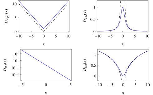
Figure 1: Functional dependencies on the position variable $x$ of the diffusion coefficients studied. The exact functional dependencies are represented by the dashed lines, while the blue curves depict the regularised forms for $D(x)$ that were used in the simulations, see text.

In addition, we analyse the behaviour of the HDP for the exponential dependence

$$D_{\mathrm{exp}}(x)=\frac{A^{2}}{2}e^{-2\alpha x},$$ (10)

such that on the left semi-axis the diffusivity increases exponentially with $|x|$, while on the positive semi-axis $D(x)$ decreases quickly. Finally, we consider the logarithmic shape

$$D_{\mathrm{log}}(x)=\frac{A^{2}}{2}\frac{1}{2}\log\left[\left(\frac{x}{\overline{x}}\right)^{2}+1\right],$$ (11)

such that a trapping region of slow diffusion is created at small $x$ where $D_{\mathrm{log}}(x)$ assumes a parabolic shape, while at $|x|\gg 1$ the diffusivity grows logarithmically like

$$D_{\mathrm{log}}(x)\sim\frac{A^{2}}{2}\log\left[\frac{|x|}{\overline{x}}\right].$$ (12)

In both cases the constants $A$ and $\alpha$ have the dimensions $\mathrm{cm}/\mathrm{sec}^{1/2}$ and $1/\mathrm{cm}$, respectively, and we set $\overline{x}=1$ below. We assume that local thermal equilibrium is established on the length-scales of spacial $D(x)$ variations. In Eq. (11) the addition of unity in the logarithm prevents the divergence to minus infinity at the origin. The exponential and logarithmic shapes for $D(x)$ are depicted in the bottom panel of Fig. 1.

Numerically, following the Stratonovich interpretation the solution of Eq. (5) requires an implicit mid-point iterative scheme for the particle displacement $x_{i}$. At the simulation step $i+1$ we thus have

$$x_{i+1}-x_{i}=\sqrt{2D([x_{i+1}+x_{i}]/2)}\leavevmode\nobreak\ (y_{i+1}-y_{i}),$$ (13)

where the increments of the Wiener process $(y_{i+1}-y_{i})$ represent a centred, $\delta$-correlated Gaussian noise with unit variance. Unit time intervals $\Delta t$ separate consecutive iteration steps in the simulations. From a set of stochastic trajectories $x(t)$ generated for an initial particle position $x(0)=x_{0}$, the ensemble and time averaged MSDs are computed. This numerical scheme has recently been implemented for HDPs with a power-law form hdp13 .

In what follows we evaluate the simulated time series $x(t)$ in terms of the ensemble averaged MSD (2), revealing different forms of sub- and superdiffusion. To analyse the ergodic properties of the HDPs, the time averaged MSD (3) is evaluated along the trajectories as function of the lag time $\Delta$. We also evaluate the additional average (4) over multiple trajectories.

For finite trajectories the time averaged MSD (3) between different trajectories will always vary. When the length $T$ of the time series reaches very large values (ideally, it is taken to infinity), the ergodicity breaking parameter he ; rytov

$$\mathrm{EB}=\lim_{T/\Delta\to\infty}\frac{\left<\left(\overline{\delta(\Delta)^{2}}\right)^{2}\right>-\left<\overline{\delta(\Delta)^{2}}\right>^{2}}{\left<\overline{\delta(\Delta)^{2}}\right>^{2}}$$ (14)

quantifies how reproducible individual realisations of the process are. At some lag time $\Delta$, a vanishing ergodicity breaking parameter is a sufficient condition for the ergodicity of a given stochastic process. A necessary condition is that the ratio of the time and ensemble averaged MSDs is unity. As such a ratio involves only the second moments, an additional ergodicity breaking parameter can be defined as

$$\mathcal{EB}=\frac{\left<\overline{\delta^{2}(\Delta,T)}\right>}{\left<x^{2}(\Delta)\right>}.$$ (15)

Although this parameter is easier to compute analytically, it may strongly depend on the initial conditions and is therefore not a universal feature of a stochastic process.

The scatter distribution for the amplitude $\overline{\delta^{2}}$ of individual trajectories around the mean $\langle\overline{\delta^{2}}\rangle$ is quantified by the distribution

$$\phi(\xi)=\phi\left(\frac{\overline{\delta^{2}}}{\langle\overline{\delta^{2}}\rangle}\right)$$ (16)

in terms of the dimensionless variable $\xi$. It characterises the randomness of individual time averaged MSDs and yields additional information in how far the diffusion process deviates from the ergodic behaviour.

For Brownian motion the finite-time scaling reads he

$$\mathrm{EB_{BM}}=\frac{4}{3}\frac{\Delta}{T}$$ (17)

for the ergodicity breaking parameter, and

$$\phi_{\text{BM}}(\xi)\to\delta(\xi-1)$$ (18)

for the amplitude scatter distribution at $T/\Delta\to\infty$. Both limiting behaviours are in excellent agreement with simulations of Brownian motion (not shown).

IV Power-law varying diffusivity

Inserting the power-law form (7) of the diffusion coefficient $D(x)$ into the diffusion equation (6), we recover the PDF hdp13

$$P(x,t)=\frac{|x|^{-\alpha/2}}{\sqrt{4\pi D_{0}t}}\exp\left(-\frac{|x|^{2-\alpha}}{(2-\alpha)^{2}D_{0}t}\right)$$ (19)

for the initial condition $P(x,0)=\delta(x)$. This equation, in turn, provides the ensemble averaged MSD

$$\langle x^{2}(t)\rangle=\Gamma\left(\frac{6-\alpha}{2(2-\alpha)}\right)\frac{\left(2-\alpha\right)^{4/(2-\alpha)}}{\pi^{1/2}}(D_{0}t)^{2/(2-\alpha)}.$$ (20)

According to Eq. (20), for $\alpha<0$ the process is subdiffusive, while superdiffusion emerges for $\alpha>0$. The limiting cases of Brownian motion with $\langle x^{2}(t)\rangle=2D_{0}t$ corresponds to $\alpha=0$, and that of ballistic motion for $\alpha=1$. The diffusion becomes increasingly fast when $\alpha$ increases towards the limiting value 2. The PDF (19) corresponds to a compressed Gaussian in the subdiffusive case ($\alpha<0$), i.e., we obtain an exponential distribution in which the exponent of $x$ is larger than 2. In the superdiffusive case ($0<\alpha<2$) the PDF (19) becomes a stretched Gaussian. Excellent agreement is observed between the theoretical PDF (19) and the numerical solution of the diffusion equation (6), as demonstrated in Fig. 2.

Further analysis of the correlation function of consecutive increments of the HDP process reveals the anti-persistent nature for the subdiffusion case, while persistent correlations accompany the superdiffusive case hdp13 . The analytical result for the velocity-velocity correlation function can be shown to resemble the correlation function of fractional Brownian motion hdp13 .

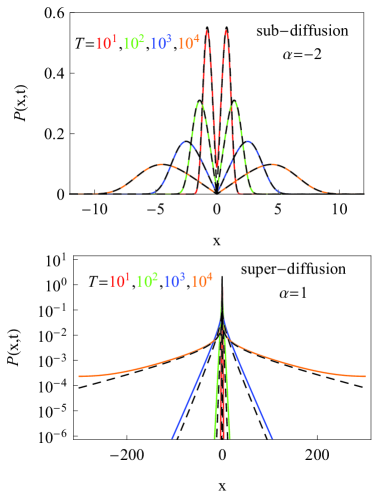
Figure 2: The PDF for sub- and superdiffusive HDPs with power-law diffusivity (7) and $D_{0}=1$. We show the analytical result (19) for different trajectory lengths $T$ (coloured lines) and the numerical solution of the dynamic equation (6), represented by the dashed lines.

The trajectory-to-trajectory averaged time averaged MSD (4) of the HDP process with power-law form (7) of the diffusion coefficient takes on a linear dependence on the lag time $\Delta$ hdp13 ,

$$\left<\overline{\delta^{2}(\Delta)}\right> = \Gamma\left(\frac{6-\alpha}{2(2-\alpha)}\right)\frac{(2-\alpha)^{4/(2-\alpha)}}{\pi^{1/2}}$$ (21)

$$\times D_{0}^{2/(2-\alpha)}\Delta T^{\alpha/(2-\alpha)}.$$

This result can be rewritten in the form

$$\left<\overline{\delta^{2}(\Delta)}\right>=\left<x^{2}(\Delta)\right>\left(\frac{\Delta}{T}\right)^{-\alpha/(2-\alpha)},$$ (22)

introducing the strong ageing dependence on the measurement time $T$: as function of the lag time the motion slows down. We can alternatively express this statement in the form $\langle\overline{\delta^{2}(\Delta)}\rangle\simeq D_{\text{ eff}}(T)\Delta$, such that this effective diffusion coefficient has the scaling

$$D_{\text{eff}}(T)\simeq T^{\frac{\alpha}{2-\alpha}}.$$ (23)

The functional relation (22) between ensemble and time averaged MSDs is identical to the one observed for subdiffusive continuous time random walk processes he as well as continuous time random walk processes with correlated waiting times vincent .

The scatter distribution $\phi\left(\overline{\delta^{2}(\Delta)}/\langle\overline{\delta^{2}(\Delta)}\rangle\right)$ in the sub- and superdiffusive cases, respectively, follows a Rayleigh-like and a generalised Gamma distribution hdp13 . Moreover for a fixed length $T$ of the underlying time series $x(t)$, the scatter distribution $\phi(\xi)$ stays nearly constant for varying lag times $\Delta$. In other words, the degree of fluctuations around the mean $\langle\overline{\delta^{2}(\Delta)}\rangle$ is approximately invariant along the HDP trajectories.

For subdiffusion with $\alpha<0$ we see from Eq. (22) that the time averaged MSD is much smaller than the ensemble averaged MSD, $\langle\overline{\delta^{2}(\Delta)}\rangle\ll\left<x^{2}(\Delta)\right>$, as long as $\Delta\ll T$. In contrast $\langle\overline{\delta^{2}(\Delta)}\rangle\gg\left<x^{2}(\Delta)\right>$ for superdiffusion with $\alpha>1$. Because of the larger amplitude spread quantified by the scatter distribution $\phi$ and its strongly asymmetric shape, the EB parameter for the case of superdiffusion is systematically larger than the one for subdiffusion: $\mathrm{EB}_{\text{super}}\approx 1.4$ compared to $\mathrm{EB}_{\text{sub}}\approx 0.4$ for $\alpha=-2$ and $\alpha=1$, respectively. This observation as well as the $\Delta$-dependence of the second EB parameter

$$\mathcal{EB}=\left(\frac{\Delta}{T}\right)^{-\alpha/(2-\alpha)}$$ (24)

are supported by computer simulations performed according to the Stratonovich scheme (not shown).

V Exponentially varying diffusivity

We now turn to the exponentially varying diffusion coefficient (10). We characterise the stochastic properties of this process with the same quantities studied above, i.e., the PDF, the time and ensemble averaged MSDs, the scatter distribution, and the ergodicity breaking parameters. In addition, we explore the initial position-induced population splitting into fast and slow walkers, the diffusion fronts, and the effective exploration of space.

Exponential distributions of the diffusion coefficient have been used to describe the motion dynamics of parasitic nematodes nematodes , or for the irradiation-enhanced diffusion of impurities where the exponential variation is effected by the decay of the radiation when it penetrates an absorbing medium irradiate . Finally, an exponential rate of morphogen degradation was applied in a reaction-subdiffusion model for cell development santos .

V.1 PDF and ensemble averaged MSD

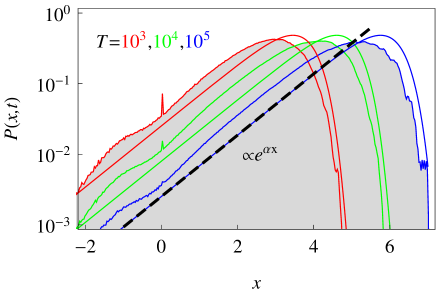
Figure 3: The universal PDF shape for HDPs with $D_{\mathrm{exp}}(x)$, obtained from simulations with initial condition $x_{0}=0$. The results are compared with the theoretical result (29). The trace lengths $T$ are indicated, and we chose $\alpha=1$ and $A=1$. The data were averaged over $N=400$ trajectories. After averaging, the PDF for short traces still contains a small spike at the initial position.

To obtain the PDF for the HDP with the exponential $x$-dependence (10), following the same steps as for the power-law form for $D(x)$ analysed in Ref. hdp13 , we employ the standard transformation of variables srokowski09

$$y(x)=\int^{x}\frac{dx^{\prime}}{\sqrt{2D_{\text{exp}}(x^{\prime})}}=\frac{\exp(\alpha x)}{\alpha A}.$$ (25)

Here $y(t)$ in the Stratonovich sense corresponds to the Wiener process, whose PDF is the standard Gaussian

$$p(y,t)=\frac{1}{\sqrt{2\pi t}}\exp\left(-\frac{y^{2}}{2t}\right),$$ (26)

Together with the normalisation condition $\int_{-\infty}^{\infty}P(x,t)dx=1$, and the probability conservation law, from Eq. (26) the normalised PDF of the HDP with exponentially varying diffusivity assumes the unimodal double-exponential form

$$P(x,t)=\frac{2}{A}\frac{\exp(\alpha x)}{\sqrt{2\pi t}}\exp\left(-\frac{1}{2t}\left[\frac{e^{\alpha x}-e^{\alpha x_{0}}}{A\alpha}\right]^{2}\right),$$ (27)

for arbitrary initial value $x_{0}$. In the limit $x\to-\infty$ the PDF of the particle after time $t$ features the exponential tail,

$$P(x,t) \sim \frac{2}{A}\frac{\exp(\alpha x)}{\sqrt{2\pi t}}\exp\left(-\frac{\exp(2\alpha x_{0})}{2tA^{2}\alpha^{2}}\right)$$ (28)

$$\sim \frac{2}{A}\frac{\exp(\alpha x)}{\sqrt{2\pi t}},$$

where in the second approximation we also took the long time limit. At large values of $x$ the PDF decays sharply in a double-exponential fashion.

For further analysis we assume that the initial condition has a sufficiently large modulus on the left semi-axis, that is, $|x_{0}|\ll(2\alpha)^{-1}$. In this case the PDF becomes

$$P(x,t)=\frac{2}{A}\frac{\exp(\alpha x)}{\sqrt{2\pi t}}\exp\left(-\frac{\exp(2\alpha x)}{2tA^{2}\alpha^{2}}\right)$$ (29)

Its maximum is located at

$$x_{\text{max}}=\frac{\log(\alpha^{2}A^{2}t)}{2\alpha},$$ (30)

where the PDF has the value

$$P(x_{\text{max}})=\sqrt{\frac{2\alpha^{2}}{\pi e}}.$$ (31)

Interestingly, the temporal shift of of the maximum position is logarithmic in time, while the value of the PDF at this maximum remains constant. We compare the functional forms (29) of the PDF with simulations results in Fig. 3, observing very favourable agreement. For the non-zero initial position $x_{0}$, the PDF is shown in Fig. 4, also exhibiting good agreement with the analytical form (27).

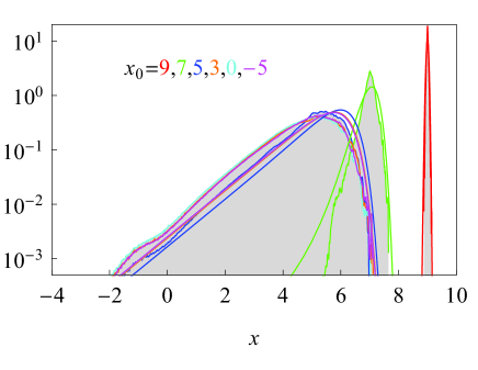
Figure 4: PDF of the HDP with $D=D_{\mathrm{exp}}(x)$ for various initial positions $x_{0}$ of the process. The smooth curves represent the theoretical result, Eq. (27). The parameters were chosen as $T=10^{5}$, $\alpha=1$, and $A=1$, and $N=400$ traces were analysed for each of the shown profiles.

The MSD may now be obtained from the PDF (29) simply by integration. The exact result reads

$$\langle x^{2}(t)\rangle=\frac{1}{4\alpha^{2}}\left(A_{1}+A_{2}\log\Big{[}\alpha^{2}A^{2}t\Big{]}+\log^{2}\Big{[}\alpha^{2}A^{2}t\Big{]}\right),$$ (32)

where $\gamma\approx 0.57721$ is the Euler-Mascheroni constant (or Euler’s constant), and we also define the two abbreviations

$$A_{1}=\pi^{2}/2+\log^{2}[2]+\gamma^{2}+2\gamma\log[2]\approx 6.55$$ (33)

and

$$A_{2}=2\gamma+2\log[2]\approx 2.54,$$ (34)

Thus, at long times $t\gg(\alpha^{2}A^{2})^{-1}$ we thus observe the logarithmic behaviour

$$\langle x^{2}(t)\rangle\sim\frac{1}{4\alpha^{2}}\log^{2}\Big{[}\alpha^{2}A^{2}t\Big{]}.$$ (35)

Formula (32) could also be obtained directly from the stochastic equation (5) in the following way. With the transformation (25) and the distribution (26) of the Wiener process, the MSD (32) results from the averaging $\int_{-\infty}^{\infty}p(y,t)x^{2}(y)dy$. We note that for general initial condition $x_{0}$ we could not find an analytical result for the MSD. Numerical analysis confirms that the MSD shows the logarithmic time dependence (32), and in the long time limit exactly converges to this form.

The logarithmic scaling of the ensemble averaged MSD (32) resembles that of other ultraslow processes. Thus, continuous time random walks with logarithmic distribution of waiting times exhibit a slow logarithmic growth of the MSD katja as well as ageing continuous time random walks lomholt . The most prominent example for logarithmic time evolution is that of Sinai diffusion, the motion of a random walker in a random force field, where the ensemble averaged MSD follows the law $\langle x^{2}_{\text{Sinai}}(t)\rangle\sim\log^{4}t$ sinaj ; doussal-sinai . Remarkably, our PDF (29) is identical to that in the Sinai model with ageing in the limit when the height of the barriers for consecutive jumps of a particle vary linearly with position. This leads to an exponential dependence of the effective diffusion coefficient and also to a $\langle x^{2}(t)\rangle\sim\log^{2}t$ scaling for the ensemble averaged MSD doussal98 .

To further quantify the dynamics of the diffusing particles, we performed stochastic simulations according to the scheme (13). From the generated trajectories $x(t)$ of the walker the PDFs were computed for different starting positions $x_{0}$ and trace lengths $T$. For negative $x_{0}$ the particles start in the domain of fast diffusion [large $D(x)$, compare Fig. 1] and rapidly escape the negative semi-axis. Typically, they become trapped on the positive semi-axis, where $D(x)$ is smaller. For large positive initial position, $x_{0}\gg 1$, the PDF is sharply peaked as the particles on average remain trapped in the region of extremely low (exponentially small) diffusivity. This peak slowly spreads for longer traces.

When $x_{0}$ becomes smaller than some ‘critical’ value, the PDF follows a universal asymmetric shape with an exponential tail at $x<0$. On the positive semi-axis, a sharp double-exponential drop-off of the PDF is observed, with a $T$-dependent location. These trends are in agreement with Eqs. (29) and (28), whose functinal form is compared with the simulations results in Fig. 4. For longer $T$, the maximum of the PDF shifts to larger $x$ values, in agreement with the theoretical prediction (30), compare Fig. 3. The ensemble averaged MSD obtained from the generated trajectories closely follows the $\sim\log^{2}[t]$ asymptote given by Eq. (32). At $x_{0}\gg 1$ the ensemble averaged MSD relaxes to this asymptote at later times because the particles are initially trapped in the exponentially slow diffusion region, resulting in a $x_{0}^{2}$-plateau at short times, see Fig. 5.

V.2 Time averaged MSD

To calculate the time averaged MSD we need to obtain the position auto-correlation function, $\langle x(t_{1})x(t_{2})\rangle$. Using the two-point probability density function for the Wiener process (without loss of generality, $t_{2}>t_{1}$),

$$\pi(y_{2},t_{2}|y_{1},t_{1})=\frac{1}{\sqrt{2\pi(t_{2}-t_{1})}}\exp\left(-\frac{(y_{2}-y_{1})^{2}}{2(t_{2}-t_{1})}\right),$$ (36)

one obtains for the positional correlation that

$$\left\langle x(t)x(t+\Delta)\right\rangle = \frac{1}{4\alpha^{2}}\int_{-\infty}^{\infty}dy_{1}\int_{-\infty}^{\infty}dy_{2}$$ (37)

$$\times\log[(\alpha Ay_{1})^{2}]\log[(\alpha Ay_{2})^{2}]$$

$$\times\pi(y_{2},t+\Delta|y_{1},t)p(y_{1},t),$$

where we again use the trick of choosing a sufficiently negative initial condition for convenience. After integration we arrive at ($\Delta<t$)

$$\left<x(t)x(t+\Delta)\right>=\frac{1}{4\alpha^{2}}\left\{A_{1}-\frac{1}{2}\arctan^{2}\left[\frac{2\sqrt{\Delta t}}{t-\Delta}\right]\right\}$$ (38)

$$-\text{4\leavevmode\nobreak\ arccot}[\sqrt{\Delta/t}]\arctan[\sqrt{\Delta/t}]$$

$$+\frac{A_{2}}{2}(\log[\alpha^{2}A^{2}t]+\log[\alpha^{2}A^{2}(t+\Delta)])$$

$$+\log[\alpha^{2}A^{2}t]\log[\alpha^{2}A^{2}(t+\Delta)].$$

For $\Delta=0$ this expression coincides with the regular ensemble averaged MSD (32), as it should. The functional dependence of the positional correlations is shown in Fig. 6. In the limit $\Delta\gg t$ the position autocorrelation function (38) approaches

$$\left<x(t)x(t+\Delta)\right>\sim\frac{\frac{1}{2}A_{2}+\log\left(\alpha^{2}A^{2}t\right)}{\left[A_{1}+A_{2}\log\left(\alpha^{2}A^{2}t\right)+\log^{2}\left(\alpha^{2}A^{2}t\right)\right]^{1/2}}.$$ (39)

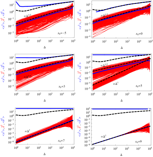
Figure 5: Ensemble averaged MSD $\langle x^{2}(t)\rangle$ (upper blue curves in each panel), time average MSD $\overline{\delta^{2}}$ of individual trajectories (red curves), and mean time averaged MSD $\langle\overline{\delta^{2}}\rangle$ (lower blue curves in each panel). The starting positions $x_{0}$ for each panel are indicated. The dashed black curves represent Eq. (32) for the ensemble averaged MSD and Eqs. (41) and (43) for the two populations, respectively. The $\overline{\delta^{2}}$ are shown with log-sampled points along the $\Delta$-axis. At $x_{0}$=5 a splitting of $\overline{\delta^{2}}$ into a slow ($\overline{\delta^{2}}\simeq\Delta^{1/2}$) and fast ($\overline{\delta^{2}}\simeq\Delta$) fraction is most pronounced. Parameters: $T=10^{5}$, $\alpha=1$, $A=1$. $N=400$ trajectories were simulated to produce the trajectory-average.

For the time averaged MSD (3) a simple scaling argument can be established in the limit of short lag times, $\Delta\ll T$. To this end, we notice that the time averaged MSD

$$\left<\overline{\delta^{2}(\Delta)}\right> = \frac{1}{T-\Delta}\int\limits_{0}^{T-\Delta}\Big{[}\left<x^{2}(t+\Delta)\right>$$ (40)

$$+\left<x^{2}(t)\right>-2\left<x(t+\Delta)x(t)\right>\Big{]}dt$$

contains three correlators in the integrand. Expanding both the MSD (32) and the two-point correlator (38) in $\Delta$, in the limit $\Delta\ll T$ we find that

$$\left<\overline{\delta^{2}(\Delta)}\right>\sim\frac{1}{T-\Delta}\int\limits_{0}^{T-\Delta}\frac{\pi}{\alpha^{2}}\sqrt{\frac{\Delta}{t}}dt\approx\frac{2\pi}{\alpha^{2}}\left({\frac{\Delta}{T}}\right)^{1/2}.$$ (41)

The square-root scaling $\langle\overline{\delta^{2}(\Delta)}\rangle\simeq\Delta^{1/2}$ is very distinct from the linear scaling observed for subdiffusive continuous time random walk processes pt ; pccp ; he as well as for time correlated continuous time random walks vincent , for ageing continuous time random walks lomholt , and for HDPs with power-law distributed diffusivities hdp13 presented in the previous Section. For initial conditions $x_{0}$ that are far away from zero on the negative semi-axis, i.e., particles starting in the high-diffusivity region, the approximate scaling (41) agrees pretty nicely with simulations results, as shown in Fig. 5.

In the opposite case of large positive $x_{0}$, the integration of Eq. (5) yields (at $\alpha x_{0}\ll 1$)

$$x(y)\approx x_{0}+e^{-\alpha x_{0}}Ay(t),$$ (42)

and after elementary averaging we find

$$\left<\overline{\delta^{2}(\Delta)}\right>\approx 2D_{\text{exp}}(x_{0})\Delta.$$ (43)

Therefore, the time averaged MSD in this limit displays the linear behaviour, that we observe for both Brownian processes as well as the above mentioned anomalous diffusion processes. The effective diffusivity naturally depends on the initial position $x_{0}$ of the particle. Eqs. (41) and (43) reveal the exponents $\frac{1}{2}$ and $1$ of the time averaged MSDs for these two extreme choices of $x_{0}$ that appear clearly distinguished in Fig. 5. We note already here that when the initial position $x_{0}$ is shifted towards more positive values, individual trajectories become more reproducible (Fig. 5), as detailed more quantitatively now.

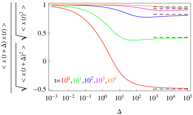
Figure 6: The normalised position correlations (37) for exponentially distributed diffusion coefficient. Parameters: $\alpha=1$ and $A=1$. The dashed lines indicates Eq. (39).

V.3 Amplitude scatter and ergodicity breaking parameter

As shown in Figs. 5 and 7, the time averaged MSD exhibits a pronounced amplitude scatter. This effect becomes increasingly stronger when the initial position is more negative, i.e., when the particle is initially placed in the high diffusivity region. For increasingly positive initial position the scatter of individual $\overline{\delta^{2}(\Delta)}$ is reduced, in the panel for $x_{0}=9$ the trajectories are almost perfectly reproducible for shorter lag times. Generally, ensemble and time averaged MSDs do not coincide (Fig. 5), a feature that clearly indicates a weak ergodicity breaking. This is further detailed in terms of the ergodicity breaking parameter in Fig. 8. The non-ergodic behaviour is due to the strong non-uniformity of the environment over typical length scales of the diffusive motion. The scaling of the time averaged MSD follows Eqs. (41) and (43) for negative and positive values of the initial positions $x_{0}$ with large modulus $|x_{0}|$, respectively (Fig. 5). For smaller modulus of the initial position $x_{0}$, the amplitude scatter of individual traces $\overline{\delta^{2}}$ becomes reduced at longer lag times $\Delta$, i.e., the width of the scatter distribution $\phi$ for the longer $\Delta$ decreases, as confirmed in Fig. 7. This phenomenon is due to the fact that when the initial condition is further left on the axis the PDFs tend to converge (Fig. 4). Thus at later stages of the trajectories the particles’ most probable location increasingly localises, thus effecting smaller scatter between individual amplitudes, i.e., smaller differences in the particle positions.

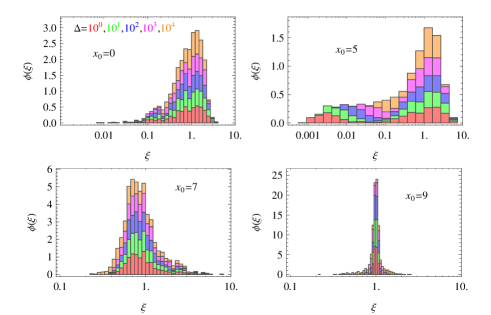
Figure 7: Amplitude scatter distribution $\phi$ of individual time averaged MSDs $\overline{\delta^{2}}$ for different initial positions $x_{0}$ for HDPs with exponentially distributed diffusion coefficient. In each panel, the colours of the stacked histograms correspond to different lag times $\Delta$ along the $\overline{\delta^{2}(\Delta)}$ traces (the bins do not overlap). In the $x_{0}=5$ panel, the $\overline{\delta^{2}}$ traces at short lag times $\Delta$ clearly split into two sub-populations (red bars), while at large $\Delta$ these two distributions merge (orange bars). The parameters are the same as in Fig. 5.

When the particle initial position is in a slow-diffusion region, $x_{0}\gg 1$, the HDP turns nearly ergodic and the amplitude scatter increases when $\Delta$ becomes comparable to the overall length $T$ of the time series. Using expression (42), one can show that the ergodicity breaking parameter (14) in the limit $\Delta\ll T$ vanishes to first order as

$$\text{EB}_{\text{exp}}\sim\frac{4}{3}\frac{\Delta}{T},$$ (44)

in agreement with computer simulations, which coincides with the result for regular Brownian motion, Eq. (17). Note, however, that despite the lack of amplitude scatter and the Brownian-style behaviour of the ergodicity breaking parameter, this process remains weakly non-ergodic due to the disparity between ensemble and time averaged MSDs. Note that for $\Delta/T\ll 1$ the HDP approaches the ergodicity differently depending on the trace length $T$. Namely, for nearly ergodic starting positions $x_{0}\gg 1$, for shorter $T$ the EB value is much closer to the Brownian asymptote, compare Fig. 8 and Fig. A1 in the Appendix.

Figure 8: Ergodicity breaking parameter as a function of the lag time for varying initial particle positions $x_{0}$ for HDPs with exponentially distributed diffusion coefficient. The parameters are the same as in Fig. 5.

V.4 Population splitting and exploration of space

Computer simulations show that at intermediate $x_{0}$ a population splitting occurs between a slow fraction following the square-root scaling of the time averaged MSD,

$$\overline{\delta^{2}(\Delta)}\simeq\Delta^{1/2}$$ (45)

and an apparently ergodic fraction with the standard linear scaling $\overline{\delta^{2}}\sim\Delta$. This is one of the the main features of the $\overline{\delta^{2}}$ traces for the case of exponential variation of the diffusion coefficient as function of the particle position $x$. Such a two-phase dynamics is observed due to the fast particles starting at $x<0$ and the nearly ergodic, slow walkers starting at $x\gg 1$. With increase of $x_{0}$ the scaling exponent $\beta$ for the initial region $\Delta\gg T$ of the trajectories,

$$\overline{\delta^{2}(\Delta\gg T)}\simeq D_{\beta}\Delta^{\beta},$$ (46)

changes from $\beta=$1/2 to $\beta$=1, as predicted by Eqs. (41) and (43) beta-note , splitting the time averaged MSD traces into two distinct populations, see Figs. 5 and 9. The diffusion coefficient $D_{\beta}$ for the initial part of the $\overline{\delta^{2}(\Delta)}$ traces is also split for intermediate $x_{0}$, see Fig. 10. Relatively large $\overline{\delta^{2}}$ amplitudes with a $\Delta^{1/2}$ scaling emerge due to fast excursions into the left semiaxis with large values of $D_{\text{exp}}(x)$. For larger $x_{0}$ the fraction of $\overline{\delta^{2}}\sim\Delta^{1}$ traces increases. Around $x_{0}$=5 the population splitting of temporal MSD is most prominent. Due to the presence of small-amplitude $\overline{\delta^{2}}$ traces linear in $\Delta$, the mean $\langle\overline{\delta^{2}}\rangle$ in the simulations is slightly lower than the theoretical $\Delta^{1/2}$-asymptote (41). Note that smaller diffusivity magnitudes $A$ have a similar effect as a larger $x_{0}$, namely, the value of the exponent $\beta$ tends to change from 1/2 to 1 as $A$ decreases (not shown).

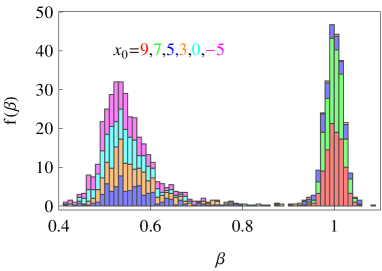
Figure 9: Evolution of the scaling exponent $\beta$ of the time averaged MSD $\overline{\delta^{2}}$ at short times for different initial positions $x_{0}$ for HDPs with exponentially varying diffusivity. A clear population splitting is observed for smaller $x_{0}=5$, with maxima centred around the predicted values $\frac{1}{2}$ and $2$ (blue bars). The parameters are the same as in Fig. 5.

This dramatic effect of the initial position $x_{0}$ affects the spreading of a packet of particles diffusing in such a medium as well as the propagation of diffusion fronts. Walkers, that are initially distributed normally according to

$$f(x)=\frac{1}{\sqrt{2\pi w^{2}}}\exp\left(-\frac{x^{2}}{2w^{2}}\right),$$ (47)

escape the region of fast diffusivity after relatively few simulations steps, due to the occurrence of relatively long jumps, that is, we observe a superdiffusive front propagation. Because of this, a peak in the normalised profiles develops at $x>0$, resembling the peak in the PDF, Fig. 11. Slow particles starting at $x_{0}\gg 1$ remain trapped in the slow-diffusion region for long times, corresponding to the nearly unaltered right wing of the distribution. Later on, the diffusion front exhibits a slow propagation reminiscent of the slow MSD scaling (32). Clearly, the traces initiated at different $x_{0}$ values will have different ergodic characteristics and the ergodic properties of the packet of diffusive particles will change upon the spatial spreading.

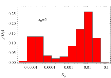
Figure 10: Population splitting of apparent diffusion coefficients for HDPs with exponentially varying diffusion coefficient, computed for the same parameters as in Fig. 5.

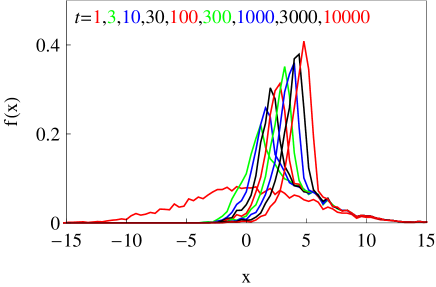
Figure 11: Focusing and propagation of a diffusing front for a packet of particles with initial normal distribution (47). We chose the parameters $w=5$ and $T=10^{4}$, and the results are averaged over $N=5000$ traces. The diffusion time $t$ is indicated in the graph.

One final dynamic characteristic of HDPs is the exploration of space. This property is relevant, for instance, for the random localisation of ‘targets’ by diffusing particles. The first-passage dynamics to such a target will be strongly affected by the target position in our strongly non-homogeneous scenario for the exponentially distributed diffusivities. The results of our simulations show that for large initial particle positions, $x_{0}\gg 1$, the space exploration is nearly symmetric and the diffusivity is small (small spread around the initial position $x_{0}$). For moderate $x_{0}>0$ excursions into the high diffusivity left semi-axis occur more frequently and earlier during the time evolution, as underlined in Fig. 12. For $x_{0}=0$ the exploration of both half-spaces is nearly equally fast. For negative $x_{0}$ with large modulus the particles quickly escape from the region of high diffusivity and the positive half-space is explored faster. The boundary of this exploration front in the positive semi-axis appears to approach a universal curve for $x_{0}\lesssim 3$.

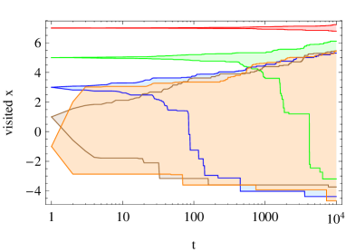
Figure 12: Space exploration by particles diffusing in a medium with exponentially distributed diffusion coefficient, shown for various initial conditions, $x_{0}=7$, 5, 3, 1, and $-1$. The trajectories are of length $T=10^{4}$.

VI Logarithmically varying diffusivity

To complete our analysis of diffusion processes with spatially varying diffusion coefficients, to contrast the previous cases of power-law and exponential variation, we now turn to the case slowly varying diffusivity. More concretely we study the HDP process with logarithmic $x$ dependence (11) of the diffusion coefficient and perform a similar analysis as pursued in the previous two Sections.

VI.1 PDF and ensemble averaged MSD

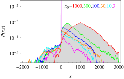
Figure 13: PDF of the HDP with logarithmically varying diffusion coefficient, computed for different initial conditions. The parameters are $T=10^{5}$, $A=1$, and $\bar{x}=1$.

Using the same change of variables for the concrete form (12) of $D(x)$ we find that ($\overline{x}=1$)

$$y(x) = \int_{x_{0}}^{x}\frac{dx^{\prime}}{\sqrt{2D_{\text{log}}(x^{\prime})}}$$ (48)

$$=\frac{2}{A}\left[x(t)F\left(\sqrt{\log x}\right)-x_{0}F\left(\sqrt{\log x_{0}}\right)\right],$$

where, we introduce Dawson’s integral

$$F(z)=e^{-z^{2}}\int_{0}^{z}e^{y^{2}}dy.$$ (49)

The PDF obtained from the PDF (26) of the Wiener process then assumes the form

$$P(x,t;x_{0}) = \frac{1}{\sqrt{2\pi tA^{2}\log x}}$$ (50)

$$\times\exp\left(-\frac{2\left[{xF\left(\sqrt{\log x}\right)-x_{0}F\left(\sqrt{\log x_{0}}\right)}\right]^{2}}{A^{2}t}\right).$$

We simulated discretised HDPs with logarithmically varying diffusion coefficient, Eq. (11). This process features a region of low diffusivity around the origin $x=0$. This region tends to trap particles diffusing in from higher diffusivity regions, and particles initially positioned close to the origin will escape this region only very slowly. The PDF thus features two maxima, as shown in Fig. 13. The first maximum is due to the initial particle position at $x=x_{0}$, while the second one at $x=0$ represents particles in the low diffusivity zone around the origin. The initial spreading can be captured by a shifted Gaussian bell curve with a renormalised diffusivity. For longer trajectories the particles accumulate progressively at $x=0$ and the PDF develops a tail at $x\gg x_{0}$, compare also Fig. 14.

These features can be quantitatively understood from the analytical shape shape (50) of the PDF. With increasing $x_{0}$, the gradient of the diffusivity $D_{\log}(x)$ on the length scale covered by the diffusing particle decreases and the HDP approaches regular Brownian motion, see also below and in Fig. 15. The trapping effect at $x=0$ becomes amplified for larger magnitudes of $A$ (not shown).

Direct numerical solution of Eq. (6) for the logarithmic form of the diffusion coefficient, Eq. (11), was obtained for moderate lengths $T$ of the time series note-num-sol . Eq. (50) describes the numerical results quite well and also agrees well with the results of our stochastic simulations, as shown in Fig. 14.

Numerical integration of the analytical expression (50) shows that the particle’s ensemble averaged MSD follows the linear Brownian time dependence, with a renormalised diffusivity and the initial value $x_{0}^{2}$,

$$\left<x^{2}(t)\right>\approx x_{0}^{2}+2D_{\text{log}}(x_{0})t.$$ (51)

This finding is is in good agreement with our stochastic simulations, see the black dashed curves in Fig. 15.

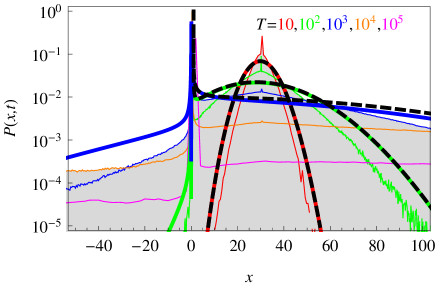
Figure 14: PDF of the HDP with logarithmic space dependence of the diffusivity, obtained from simulations with different $T$. The dashed black curves represent Eq. (50), the coloured curves correspond to numerical solution of Eq. (6). The two sets of curves agree well for short $T$. Parameters: $x_{0}=30$ and $A=1$.

VI.2 Time averaged MSD, amplitude scatter, and ergodicity breaking

The particle displacement $x(y)$ for the logarithmic dependence of the diffusion coefficient is a non-trivial function of the Wiener process $y(t)$, as demonstrated by Eq. (48), and it is hard to get a general expression for $\overline{\delta^{2}(\Delta)}$. In the short time limit $t\to 0$, however, expanding Dawson’s integral for $|x-x_{0}|\ll 1$, one finds a linear relation of $x(y)$, namely,

$$x(t)\approx x_{0}+\log^{1/2}[x_{0}]Ay(t).$$ (52)

This relation resembles Eq. (42) for the case of exponentially varying diffusivity. Then, using Eq. (37), the position correlations become

$$\left\langle x(t)x(t+\Delta)\right\rangle=\left\langle x^{2}(t)\right\rangle\approx x_{0}^{2}+\log[x_{0}]A^{2}\Delta.$$ (53)

In this limit, the time averaged MSD is a linear function of the lag time $\Delta$ with an effective diffusivity depending on the initial particle position,

$$\left<\overline{\delta^{2}(\Delta)}\right>\approx 2D_{\text{log}}(x_{0})\Delta.$$ (54)

This linear scaling is identical with the result Eq. (43) for exponentially varying diffusivity. It is also in agreement with computer simulations for $x_{0}\gg 1$, as shown in Fig. 15. In this regime, the ergodicity breaking parameter vanishes in the limit $\Delta/T\to 0$.

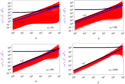
Figure 15: Ensemble and time averaged MSDs of individual trajectories for the HDP with logarithmically varying diffusion coefficient. The black dashed lines represent Eq. (51) for $\langle x^{2}\rangle$ and Eq. (54) for $\langle\overline{\delta^{2}}\rangle$. The parameters are the same as in Fig. 13.

In contrast to the initial plateau $x_{0}^{2}$ of the ensemble averaged MSD (51), the time averaged MSD $\overline{\delta^{2}}$ starts linearly in the lag time $\Delta$ and in fact stays linear for those particles, that do not become trapped. The particles that eventually do become trapped in the low-diffusivity zone give rise to a stalling of the time averaged MSD $\overline{\delta^{2}}$ so that we observe a population splitting between mobile and immobile fractions with local scaling exponents $\beta\approx 1$ and $\beta\approx 0$, respectively. Trapping is obviously strongest for small $x_{0}$, for which the spread of the temporal MSD is also the largest. Due to these immobile particles, the analytical value (54) is higher than the actual value $\langle\overline{\delta^{2}}\rangle$ from the simulations (Fig. 15). Such particle immobilisation and its effect on $\langle\overline{\delta^{2}}\rangle$ is similar to that observed for continuous time random walks with ageing johannes , see discussion in Sec. VII.

For more remote initial positions, $x_{0}\gg 1$ the ‘diffusion trap’ at $x=0$ is not strong enough, the fraction of normal traces $\overline{\delta^{2}}\sim\Delta$ grows, and $\langle\overline{\delta^{2}}\rangle$ is nicely described by Eq. (54), compare the dashed black line in Fig. 15. At smaller $A$, the trapping propensity of the trap is impeded (not shown).

The amplitude scatter distribution of individual traces $\overline{\delta^{2}}$ is broad for small values of the initial position $x_{0}$, as demonstrated in Fig. 16. The distribution in fact also exhibits a certain bi-modality due to the population splitting into mobile and immobile particles. For longer lag times $\Delta$ the fraction of trapped particles increases and the peak of the scatter distribution around $\overline{\delta^{2}(\Delta)}=0$ becomes more pronounced. The local scaling exponent $\beta$, however, is predominantly unimodal and centred around unity for larger values of $x_{0}$, compare the histograms in Fig. 17.

Figure 16: Amplitude scatter of the time averaged MSD $\overline{\delta^{2}}$ for different initial positions $x_{0}$ for the HDP with logarithmic varying diffusion coefficient. In this plot, bins of stacked histograms do not overlap. The fraction of traces with small magnitudes of $\overline{\delta^{2}}$ grows as $x_{0}$ decreases. The parameters are the same as in Fig. 13.

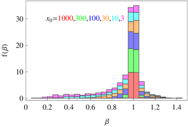
Figure 17: Apparent scaling exponent of the initial behaviour of the time averaged MSD $\overline{\delta^{2}}$ revealing a greater spread at small $x_{0}$, for which the fraction of trapped trajectories is larger. The parameters are the same as in Fig. 13.

Fig. 18 illustrates the non-ergodic nature of HDPs with logarithmic $x$-dependence of the diffusivity. We observe that for small modulus of the initial position $x_{0}$ a substantial fraction of particles is trapped at $x$=0 and the ergodicity breaking parameter (14) is relatively large, namely, $\mathrm{EB}\gg 1$ eb1-vs-eb2 . For $x_{0}\gg 1$ the HDP is nearly ergodic, recovering the self-averaging property of normal diffusion. Note that as the length $T$ of the time series grows, the HDP approaches the ergodic behaviour at considerably larger $x_{0}$ values, compare Fig. 18 as well as Fig. A2 in the Appendix.

Figure 18: Ergodicity breaking parameter EB for logarithmically varying diffusion coefficient. It approaches the Brownian behaviour (17) for large values of the initial position $x_{0}$. The parameters are the same as in Fig. 13.

We conclude this Section with the analysis of the survival probability $S(t)$, that measures the fraction of particles remaining mobile as function of the diffusion time $t$. This survival probability is thus a dynamic characteristic for the immobilisation of particles over time in the trapping potential effected by the form (11) of the diffusion coefficient. As discussed above, at small initial distances $x_{0}$ from the capturing well, the fraction of stalled walkers grows. For larger $x_{0}$, a larger fraction of particles remain mobile, corresponding to a larger value of $S(t)$ at the same time $t$. This behaviour is shown in Fig. 19. Computer simulations show that, independent of the starting position, the survival probability decreases for long times as

$$S(t)\sim\frac{1}{\sqrt{t}},$$ (55)

see the dashed line in Fig. 19 representing the inverse square root scaling. For particles starting at larger $x_{0}$ the onset of this scaling is naturally delayed to longer times $t$.

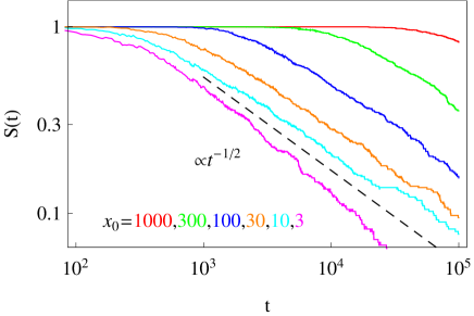
Figure 19: Survival probability of non-trapped particles for $D=D_{\text{log}}(x)$. Starting positions $x_{0}$ are indicated. The length of the trajectories is $T=10^{5}$. Walkers with an amplitude smaller than the cutoff $x_{\star}=10^{-5}$ are considered trapped.

VII Conclusions and Outlook

We analysed a model for HDPs with distance-dependent diffusivities that exhibit sub-, super-, and ultra-slow diffusion as well as weak ergodicity breaking. Power-law, exponential and logarithmic variations of the diffusion coefficient were examined. This framework can be applied to other variants of the spatial dependence $D(x)$ of the diffusion coefficient note-stretched-exp . Our results may find applications in a wide variety of spatially heterogeneous media. A particular example is the viral infection dynamics, as a mathematical rational to discriminate nearly Brownian and anomalous populations of diffusing viral particles, which was observed by single particle tracking in living bacteria seisen01 . For this purpose, an extension of the analytical and computational schemes for HDPs in higher dimensions is currently in progress inprep .

In particular, for an exponentially varying diffusivity we showed that the initial condition of the system have a vital impact on the time dependence of the process. Specifically, depending on the gradient of the particle diffusivity over the first steps of a trajectory, the scaling of the temporal MSD may become anomalous [$\overline{\delta^{2}(\Delta)}\simeq\Delta^{1/2}$] and thus lead to a population splitting compared with the traces with linear scaling [$\overline{\delta^{2}(\Delta)}\simeq\Delta$]. The time averaged traces with this anomalous scaling $\overline{\delta^{2}(\Delta)}\sim\Delta^{1/2}$ progressively drive the system toward stronger deviations from ergodicity. We also examined the asymmetry in the spatial exploration patterns, which will affect the efficiency of diffusion limited processes in such a medium.

For the case of a logarithmically varying diffusion coefficient with an associated trap of vanishing diffusivity at the origin, we also observed weakly non-ergodic behaviour with split populations with respect to the time averaged MSD $\overline{\delta^{2}}$. Here, stalled traces with $\overline{\delta^{2}(\Delta)}\sim\mathrm{const.}$ separate from mobile ones. For particles starting far from the trap at the origin, however, the ensemble and time averaged characteristics can be captured in terms of a Brownian-style motion with renormalised diffusivity $D(x_{0})$.

Let us contrast these observations with the results of the subdiffusive continuous time random walk model, compare Ref. pccp . Due to the underlying long tailed distribution of trapping times $\tau$, $\psi(\tau)\sim\tau^{-(1+\alpha)}$ with $0<\alpha<1$, the characteristic waiting time $\langle\tau\rangle$ for this system diverges. The ergodicity breaking then occurs naturally because the lack of a finite microscopic time scale $\langle\tau\rangle$ negates the existence of a long measurement time $T$ limit and thus the system remains non-stationary. For the HDPs considered here, the violation of ergodicity is solely due to the spatial variation of the diffusion process, and the anomalous diffusion is due to the multiplicative nature of the noise.

Regarding the population splitting in terms of the time averaged MSD $\overline{\delta^{2}}$, we note that a similar effect was recently analysed for continuous time random walks in the presence of strong ageing johannes . In that case the proportion of immobile versus trapped walkers was shown to grow with the age $t_{a}$ of the process. Concurrently, the ergodicity breaking parameter for such strong ageing diverges for $t_{a}\gg T$ in the form $\mathrm{EB}\sim(t_{a}/T)^{-(1+\alpha)}$, while for the population of exclusively mobile particles one finds $0<\text{EB}_{m}\leq 1$ in the same limit johannes . For HDPs with exponential variation of the diffusivity we similarly observe that the trapped particles contribute large values to the $\mathrm{EB}$ parameter, while slowly but normally diffusing particles far from the trap remain nearly ergodic.

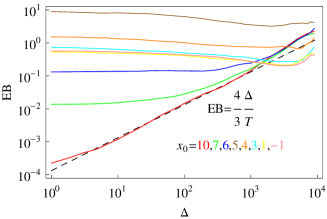
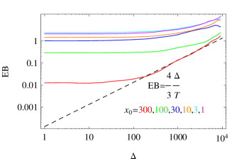
Figure 20: Left: Ergodicity breaking parameter for $D=D_{\text{exp}}(x)$ and Right: Ergodicity breaking parameter for $D=D_{\text{log}}(x)$, both for $T=10^{4}$.

Experimentally, a coexistence of ergodic and non-ergodic diffusion pathways was observed for the motion of ion channels in plasma membranes and of insulin granules in the cytosol of living cells weigel . Similarly, direct tracking of proteins and cajal bodies diffusing in the cell nucleus revealed the existence of two particle populations with distinct mobilities kubi01 ; platani . Strongly restricted diffusion in the crowded nucleus environment, with normal and anomalous components possibly occurring on different length- and time-scales, may produce such a separation effect.

Appendix A Ergodicity breaking parameter for shorter trajectories

To illustrate the approach to ergodicity, we present graphs for the ergodicity breaking parameter for trajectories, that are 10 times shorter than those used in the the majority of Figures in the main text. These Figures are referenced in the main text.

References

- (1) J.-P. Bouchaud and A. Georges, Phys. Rep. 195, 127 (1990).
- (2) R. Metzler and J. Klafter, Phys. Rep. 339, 1 (2000); J. Phys. A 37, R161 (2004).
- (3) H. Scher and E. W. Montroll, Phys. Rev. B 12, 2455 (1975).
- (4) F. Amblard, A. C. Maggs, B. Yurke, A. N. Pargellis, and S. Leibler, Phys. Rev. Lett. 77, 4470 (1996).
- (5) I. Y. Wong, M. L. Gardel, D. R. Reichman, E. R. Weeks, M. T. Valentine, A. R. Bausch, and D. A. Weitz, Phys. Rev. Lett. 92, 178101 (2004).
- (6) Q. Xu, L. Feng, R. Sha, N. C. Seeman, and P. M. Chaikin, Phys. Rev. Lett. 106, 228102 (2011).
- (7) H. Scher, G. Margolin, R. Metzler, J. Klafter, and B. Berkowitz, Geophys. Res. Lett. 29, 1061 (2002).
- (8) T. H. Solomon, E. R. Weeks, and H. L. Swinney, Phys. Rev. Lett. 71, 3975 (1993).
- (9) S. Stapf, R. Kimmich, and R.-O. Seitter, Phys. Rev. Lett. 75, 2855 (1995).
- (10) A. Ott, J.-P. Bouchaud, D. Langevin, and W. Urbakh, Phys. Rev. Lett. 65, 2201 (1990).
- (11) E. Barkai, Y. Garini, and R. Metzler, Phys. Today 65, 29 (2012).
- (12) M. J. Saxton, Biophys. J. 72, 1744 (1997); M. J. Saxton and K. Jacobson, Annu. Rev. Biophys. Biomol. Struct. 26, 373 (1997).
- (13) F. Höfling and T. Franosch, Rep. Prog. Phys. 76, 046602 (2013).
- (14) P. C. Bressloff and J. M. Newby, Rev. Mod. Phys. 85, 135 (2013).
- (15) S. Yamada, D. Wirtz, and S. C. Kuo, Biophys. J. 78, 1736 (2000).
- (16) J.-H. Jeon, V. Tejedor, S. Burov, E. Barkai, C. Selhuber-Unkel, K. Berg-Sørensen, L. Oddershede, and R. Metzler, Phys. Rev. Lett. 106, 048103 (2011).
- (17) S. M. A. Tabei, S. Burov, H. Y. Kim, A. Kuznetsov, T. Huynh, J. Jureller, L. H. Philipson, A. R. Dinner, and N. F. Scherer, Proc. Natl. Acad. Sci. USA 110, 4911 (2013).
- (18) M. A. Taylor, J. Janousek, V. Daria, J. Knittel, B. Hage, H.-A. Bachor, and W. P. Bowen, Nature Photonics 7, 229 (2013).
- (19) I. Golding and E. C. Cox, Phys. Rev. Lett. 96 098102 (2006).
- (20) S. C. Weber, A. J. Spakowitz, and J. A. Theriot, Phys. Rev. Lett. 104, 238102 (2010).
- (21) I. Bronstein, Y. Israel, E. Kepten, S. Mai, Y. Shav-Tal, E. Barkai, and Y. Garini, Phys. Rev. Lett. 103, 018102 (2009).
- (22) G. Guigas, C. Kalla, and M. Weiss, Biophys. J. 93, 316 (2007).
- (23) A. Caspi, R. Granek and M. Elbaum, Phys. Rev. Lett. 85, 5655 (2000); Phys. Rev. E 66, 011916 (2002).
- (24) G. Seisenberger, M. U. Ried, T. Endreß, H. Büning, M. Hallek, and C. Bräuchle, Science 294, 1929 (2001).
- (25) C. Brauchle, G. Seisenberger, T. Endreß, M. U. Ried, H. Büning, and M. Hallek, Chem. Phys. Chem. 3, 299 (2002).
- (26) L. Bruno, V. Levi, M. Brunstein, M. A. Desposito, Phys. Rev. E 80, 011912 (2009).
- (27) D. S. Banks and C. Fradin, Biophys. J. 89, 2960 (2005).
- (28) A. V. Weigel, B. Simon, M. M. Tamkun, and D. Krapf, Proc. Nat. Acad. Sci. USA 108, 6438 (2011).
- (29) M. Weiss, H. Hashimoto, and T. Nilsson, Biophys. J. 84, 4043 (2003).
- (30) J.-H. Jeon, H. Martinez-Seara Monne, M. Javanainen, and R. Metzler, Phys. Rev. Lett. 109, 188103 (2012); M. Javanainen, H. Hammaren, L. Monticelli, J.-H. Jeon, R. Metzler, and I. Vattulainen, Faraday Disc. 161, 397 (2013).
- (31) G. R. Kneller, K. Baczynski, and M. Pasenkiewicz-Gierula, J. Chem. Phys. 135, 141105 (2011).
- (32) T. Akimoto, E. Yamamoto, K. Yasuoka, Y. Hirano, and M. Yasui, Phys. Rev. Lett. 107, 178103 (2011).
- (33) D. Robert, T.-H. Nguyen, F. Gallet, and C. Wilhelm, PLoS ONE 4, e10046 (2010).
- (34) I. M. Sokolov, Soft Matter 8, 9043 (2012).
- (35) S. Burov, J.-H. Jeon, R. Metzler, and E. Barkai, Phys. Chem. Chem. Phys. 13, 1800 (2011).
- (36) I. Goychuk, Phys. Rev. E 80, 046125 (2009); Adv. Chem. Phys. 150, 187 (2012).
- (37) E. W. Montroll and G. H. Weiss, J. Math. Phys. 6, 167 (1965).
- (38) R. Metzler, E. Barkai, and J. Klafter, Phys. Rev. Lett. 82, 3563 (1999).
- (39) J.-H. Jeon, E. Barkai, and R. Metzler, J. Chem. Phys. (at press).
- (40) B. B. Mandelbrot and J. W. van Ness, SIAM Rev. 1, 42 (1968); A. N. Kolmogorov, Dokl. Acad. Sci. USSR 26, 115 (1940).
- (41) E. Lutz, Phys. Rev. E 64, 051106 (2001).
- (42) D. Ernst, M. Hellmann, J. Köhler, and M. Weiss, Soft Matter 8, 4886 (2012).
- (43) A. Fuliński, Phys. Rev. E 83, 061140 (2011); J. Chem. Phys. 138, 021101 (2013).
- (44) S. Havlin and D. Ben-Avraham, Adv. Phys. 36, 695 (1987).
- (45) A. Klemm, R. Metzler, and R. Kimmich, Phys. Rev. E 65, 021112 (2002).
- (46) M. F. Shlesinger, J. Klafter, and Y. M. Wong, J. Stat. Phys. 27, 499 (1982)
- (47) M. Niemann, H. Kantz, and E. Barkai, Phys. Rev. Lett. 110, 140603 (2013).
- (48) G. Zumofen and J. Klafter, Phys. Rev. E 51, 1818 (1995); ibid. 47, 851 (1993).
- (49) A. Godec and R. Metzler, Phys. Rev. Lett. 110, 020603 (2013); Phys. Rev. E 88, 012116 (2013); D. Froemberg and E. Barkai, Phys. Rev. E 87, 030104(R) (2013); E-print arXiv:1306.2036.
- (50) B. P. English, V. Hauryliuk, A. Sanamrad, S. Tankov, N. H. Dekker, and J. Elf, Proc. Natl. Acad. Sci. 108, E365 (2011).
- (51) T. Kühn, T. O. Ihalainen, J. Hyväluoma, N. Dross, S. F. Willman, J. Langowski, M. Vihinen-Ranta, and J. Timonen, PLoS One 6, e22962 (2011).
- (52) M. Platani, I. Goldberg, A. I. Lamond, and J. R. Swedlow, Nature Cell Biol. 4, 502 (2002).
- (53) R. Haggerty and S. M. Gorelick, Water Res. Res. 31, 2383 (1995).
- (54) M. Dentz, P. Gouze, A. Russian, J. Dweik, and F. Delay, Adv. Water Res. 49, 13 (2012).
- (55) T. Srokowski and A. Kaminska, Phys. Rev. E 74, 021103 (2006).
- (56) T. Srokowski, Phys. Rev. E 78, 031135 (2008).
- (57) A. T. Silva, E. K. Lenzi, L. R. Evangelista, M. K. Lenzi, H. V. Ribero, and A. A. Tateishi, J. Math. Phys., 52 083301 (2011).
- (58) A. V. Chechkin, R. Gorenflo and I. M. Sokolov, J. Phys. A: Math. Gen. 38, L679 (2005).
- (59) L. F. Richardson, Proc. Roy. Soc. London, Ser. A 110, 709 (1926); A. S. Monin and A. M. Yaglom, Statistical Fluid Mechanics (MIT Press, Cambdridge MA, 1971).
- (60) B. O’Shaughnessy and I. Procaccia, Phys. Rev. Lett. 54, 455 (1985).
- (61) Y. Meroz, I. Eliazar, and J. Klafter, J. Phys. A 42, 434012 (2009); Y. Meroz, I. M. Sokolov, and J. Klafter, Phys. Rev. Lett. 110, 090601 (2013).
- (62) A. G. Cherstvy, A. V. Chechkin, and R. Metzler, http://arxiv.org/abs/1303.5533
- (63) J.-P. Bouchaud, J. Phys. I (Paris) 2, 1705 (1992); G. Bel and E. Barkai, Phys. Rev. Lett. 94, 240602; A. Rebenshtok and E. Barkai, ibid. 99, 210601 (2007); M. A. Lomholt, I. M. Zaid, and R. Metzler, Phys. Rev. Lett. 98, 200603 (2007).
- (64) Y. He, S. Burov, R. Metzler and E. Barkai, Phys. Rev. Lett. 101, 058101 (2008).
- (65) A. Lubelski, I. M. Sokolov, and J. Klafter, Phys. Rev. Lett. 100, 250602 (2008).
- (66) S. Burov, R. Metzler, and E. Barkai, Proc. Natl. Acad. Sci. USA 107, 13228 (2010).
- (67) J. H. P. Schulz, E. Barkai, and R. Metzler, Phys. Rev. Lett. 110, 020602 (2013); E. Barkai, ibid. 90, 104101 (2003).
- (68) M. Magdziarz, R. Metzler, W. Szczotka, and P. Zebrowski, Phys. Rev. E 85, 051103 (2012); V. Tejedor and R. Metzler, J. Phys. A 43, 082002 (2010).
- (69) M. A. Lomholt, L. Lizana, R. Metzler, and T. Ambjörnsson, Phys. Rev. Lett. 110, 208301 (2013).
- (70) W. Deng and E. Barkai, Phys. Rev. E 79, 011112 (2009).
- (71) J.-H. Jeon and R. Metzler, Phys. Rev. E 85, 021147 (2012); J.-H. Jeon, N. Leijnse, L. B. Oddershede, and R. Metzler, New J. Phys. 15, 045011 (2013).
- (72) S. Condamin, V. Tejedor, R. Voituriez, O. Bénichou, and J. Klafter, Proc. Natl. Acad. Sci. USA 105, 5675 (2008).
- (73) V. Tejedor, O. Bénichou, R. Voituriez, R. Jungmann, F. Simmel, C. Selhuber-Unkel, L. Oddershede, and R. Metzler, Biophys. J. 98, 1364 (2010).
- (74) M. Magdziarz, A. Weron, K. Burnecki, and J. Klafter, Phys. Rev. Lett. 103, 180602 (2009); M. Magdziarz and J. Klafter, Phys. Rev. E 82, 011129 (2010).
- (75) K. Burnecki, E. Kepten, J. Janczura, I. Bronshtein, Y. Garini, and A. Weron, Biophys. J. 103, 1839 (2012).
- (76) A. Robson, K. Burrage, and M. C. Leake, Trans. Roy. Soc. B 368, 20120029 (2013).
- (77) H. Risken, The Fokker-Planck Equation, (Springer, Heidelberg, 1989).
- (78) S. M. Rytov, Introduction to Statistical Radio-Physics (Defense Technical Information Center, Moscow, 1968).
- (79) S. Hapca, J. W. Crawford, K. MacMillan, M. J. Wilson, and L. M. Young, J. Theoret. Biol. 248, 212 (2007); S. Hapca, J. W. Crawford, and L. M. Young, J. Roy. Soc. Interfaces 6, 111 (2009).
- (80) J. Kowall, D. Peak, and J. W. Corbett, Phys. Rev. B 13, 477 (1976); A. G. Kesarev and V. V. Kondrat’ev, Phys. Metals & Metallogr. 108, 30 (2009).
- (81) S. B. Yuste, E. Abad, and K. Lindenberg, Phys. Rev. E 82, 061123 (2010).
- (82) T. Srokowski, Phys. Rev. E 79, 040104 (2009).
- (83) S. I. Denisov, S. B. Yuste, Y. S. Bystrik, H. Kantz, and K. Lindenberg, Phys. Rev. E 84, 061143 (2011); S. I. Denisov, Yu. Bystrik, and H. Kantz, ibid. 87, 022117 (2013); J. Dräger and J. Klafter, Phys. Rev. Lett. 84, 5998 (2000).
- (84) Ya. G. Sinai, Theory Prob. Appl. 27, 256 (1982).
- (85) P. Le Doussal et al., Phys. Rev. E 59, 4795 (1999).
- (86) L. Laloux and P. Le Doussal et al., Phys. Rev. E 57, 6296 (1998).
- (87) To determine the exponent of scaling at , we first remove the last decade of temporal traces to improve the statistics. The remaining long trace is divided into two equal parts in the log-scale for . Fitting the initial part of with log-sampled points by gives the starting exponent .
- (88) The outcomes are almost insensitive to the choice of boundary conditions in the simulation box and the PDF keeps its norm, in contrast to the same computation scheme applied to the strongly asymmetric case.
- (89) Here we distinguish the two ergodicity breaking parameters, Eqs. (14) and (15). The first one is the sufficient condition of ergodicity, it involves only temporal moments and is a robust characteristics of the process. The second one operates with 2nd moments for ensemble and time averaged MSDs and therefore is a function of initial conditions. From Fig. 18 we observe e.g. that at , while the canonical parameter is far away from its ergodic value . In contrast, at large we get that because of large starting at with and small amplitude. The EB parameter follows however closely the Brownian law (17) in a large region of .
- (90) We have performed a similar type of analysis for other exponentially varying forms of the diffusion coefficient, e.g., for a stretched exponential . In the case of for instance, the PDF exhibits two symmetric peaks. The scaling of traces depends on the particle starting position . For near a peak of PDF, the particle stays effectively trapped that results in small magnitudes. For the particles jumping between the PDF peaks, the variation in position is large and so is the magnitude. The population splitting of temporal MSDs takes place due to the existence of these two diffusion pathways. Initially, we observe a linear growth , while for the later stages of the trajectory a crossover to scaling takes place.
- (91) A. G. Cherstvy, A. V. Chechkin, and R. Metzler (unpublished).
- (92) T. Kues, R. Peters, and U. Kubitscheck, Biophys. J. 80, 2954 (2001).