Spin Drag of a Fermi Gas in a Harmonic Trap

Abstract

Using a Boltzmann equation approach, we analyze how the spin drag of a trapped interacting fermionic mixture is influenced by the non-homogeneity of the system in a classical regime where the temperature is much larger than the Fermi temperature. We show that for very elongated geometries, the spin damping rate can be related to the spin conductance of an infinitely long cylinder. We characterize analytically the spin conductance both in the hydrodynamic and collisionless limits and discuss the influence of the velocity profile. Our results are in good agreement with recent experiments and provide a quantitative benchmark for further studies of spin drag in ultracold gases.

In the recent years, ultracold atoms have become a unique testing ground for quantum many-body physics. Their study has favored the emergence of novel experimental and theoretical techniques which have led to an accurate quantitative understanding of the thermodynamic properties of strongly correlated dilute gases at equilibrium Zwerger (2012). An important effort is now devoted to the exploration of the out-of-equilibrium behavior of these systems, and in particular to the determination of their transport properties. For instance, recent experiments have probed the transport of an ultracold sample through a mesoscopic channel Brantut et al. (2012), and time of flight expansions have been used to measure the gas viscosity in the strongly correlated regime Cao et al. (2011) where it is predicted to be close to the universal limit conjectured by string theory Kovtun et al. (2005).

In this Letter we focus on spin transport properties of a Fermi gas which have now received considerable attention in the cold atom community Liao et al. (2011); Bruun (2012); Enss and Haussmann (2012); Wong et al. (2012); Heiselberg (2012); Kittinaradorn et al. (2012); Kim and Huse (2012) after previously being studied in the context of liquid ³He Musaelian and Meyerovich (1992), ferromagnetic metals Mineev (2004) and spintronic materials Wolf et al. (2001). Recent measurements of the spin drag coefficient Sommer et al. (2011a, b) have shown that the most challenging aspect of these studies is how to extract the homogeneous gas properties from measurements performed in harmonic traps. The trapping potential creates a density inhomogeneity which can significantly alter the transport behaviour of the gas, because the local mean free path can vary strongly from point to point in the trap leading to a coexistence of regions, from hydrodynamic near the cloud center to collisionless at the edge Bruun and Pethick (2011). For the same reason, the velocity during the relaxation to equilibrium is not constant as a function of radius and it is essential that it be accurately known in order to find the correct values of transport coefficients. Previous theoretical attempts to cope with these problems have included making unverified assumptions about the velocity profile of the gas Vichi and Stringari (1999); Chiacchiera et al. (2010); Bruun (2011) or treating the problem in the hydrodynamic approximation with spatially varying spin diffusivity Bruun and Pethick (2011). In this last work, no quantitative conclusion could be obtained due to the importance of the collisionless regions of the cloud.

Here we present a systematic study of the spin transport in an elongated harmonic trap based on the Boltzmann equation using a combination of analytical and numerical methods in the dilute limit and for small phase-space density. In this regime we are able to analyze the behavior of the trapped gas, allowing us to deal ab initio with the spatial density changes without any uncontrolled approximations. In particular we are able to make definite predictions for the spin drag coefficient and the transverse velocity profile in both the collisionless and hydrodynamic regimes. Due to the fact that the trapping is much weaker in the axial than the radial direction, we can use the local density approximation to relate the local spin conductance in each slice perpendicular to the axis of the trap to the spin conductance in an infinite trap with the same central density.

Consider an ensemble of spin $1/2$ fermions of mass $m$ confined in a very elongated harmonic trap with axial frequency $\omega_{z}$ and transverse frequency $\omega_{x}=\omega_{y}\equiv\omega_{\perp}\gg\omega_{z}$. Each atom has $s=\pm$ spin with equal numbers of atoms in each spin state. In the initial thermal equilibrium state the two spin species are separated from each other by an average distance of $\pm z_{0}$ along the symmetry axis of the trap as in Sommer et al. (2011a). Then we let the system relax towards equilibrium and, as observed experimentally, the relaxation of the motion of the centers of mass of the two clouds occurs at a rate $\propto\omega_{z}^{2}/\gamma_{\rm coll}$, where $\gamma_{\rm coll}$ is the collision rate Sommer et al. (2011a). In the very elongated limit $\omega_{z}\ll\omega_{\perp},\gamma_{\rm coll}$ the momentum and spatial transverse degrees of freedom are therefore always thermalized and we can assume that the phase space density of the spin species $s=\pm$ is given by the ansatz

$$f_{s}(\bm{r},\bm{p},t)=f_{0}(\bm{r},\bm{p})(1+s\alpha(z,t)),$$ (1)

where $f_{0}$ is the equilibrium phase-space density. As long as interparticle correlations are weak, the single particle phase space density encapsulates all the statistical information on the system. In the rest of the Letter we will restrict ourselves to such a regime. Since the experiment Sommer et al. (2011a) was performed at unitarity, this condition is achieved when the temperature is much larger than the Fermi temperature. As a consequence, we can also neglect Pauli blocking during collisions.

Let $\bar{n}_{s}(z,t)=\int d^{2}\bm{\rho}d^{3}\bm{p}f_{s}(\bm{r},\bm{p},t)=\bar{n}_{0}(z)(1+s\alpha(z,t))$ be the 1D-density along the axis of the trap, where $\bm{\rho}=(x,y)$. Due to particle number conservation we have

$$\partial_{t}\bar{n}_{s}+\partial_{z}\Phi_{s}=0,$$ (2)

where $\Phi_{s}=\int d^{2}\bm{\rho}d^{3}\bm{p}f_{s}(\bm{r},\bm{p})v_{z}$ (with $v_{z}=p_{z}/m$, the axial velocity) is the particle flux of spin $s$ in the $z$ direction. If the trap is very elongated we can define a length scale $\ell$ much smaller than the axial size of the cloud, but much larger than its transverse radius, the interparticle distance or the collisional mean-free path so that for distances smaller than $\ell$ along the $z$ axis, the physics can be viewed as being equivalent to that of an infinitely elongated trap ($\omega_{z}=0$) with the same central density. In this setup the two spin species are pulled apart by a force $\bm{F}_{s}=-\bm{\nabla}V-(\bm{\nabla}P_{s})/n_{s}$ where $V$ is the spin independent trapping potential, $P_{s}$ is the pressure of the spin species $s$ and $n_{s}(\bm{r},t)=\int d^{3}\bm{p}f_{s}(\bm{r},\bm{p},t)$ is the associated density. We consider here a classical ideal gas, for which $P_{s}=nsk_{B}T$. Using the ansatz (1), we see that the force field is uniform and is given by $\bm{F}_{s}=-sk_{B}T\partial_{z}\alpha\bm{e}_{z}\equiv F_{s}\bm{e}_{z}$, where $\bm{e}_{z}$ is the unit vector along $z$, since $\partial_{z}\alpha$ can be considered constant to leading order on the length scale $\ell$.

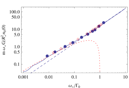
Figure 1: Color online. Spin conductance $G$ vs. $\omega_{\perp}/\Gamma_{0}$. The blue dashed line corresponds to the collisionless limit $G\simeq 15.87n_{0}/\Gamma_{0}$ for a Maxwellian gas while the red-dotted line is the hydrodynamic prediction $G\simeq(2\pi n_{0}/\Gamma_{0})\ln\Gamma_{0}$. The solid line is the semi-analytical prediction for the Maxwellian gas (see Supplemental Material). The blue dots are the results of the molecular dynamics simulation for a constant cross-section. The red open diamonds correspond to a momentum dependent cross-section with $k_{\rm th}a=2$, where $k_{\rm th}=\sqrt{mk_{B}T/\hbar^{2}}$ is the thermal wavevector.

In the regime of linear response, the particle flux is proportional to the drag force and we can write $\Phi_{s}=GF_{s}$, where $G$ is the “spin conductance” that a priori depends on the 1D-density of the cloud. Inserting this law in Eq. (2) and substituting $\alpha(z,t)=e^{-\gamma t}\alpha_{0}(z)$, which corresponds to the exponential decay of the perturbation close to equilibrium, we see that $\alpha_{0}$ is solution of

$$\gamma\bar{n}_{0}(z)\alpha_{0}(z)+k_{B}T\partial_{z}\left(G(\bar{n}_{0}(z))\partial_{z}\alpha_{0}(z)\right)=0.$$ (3)

The exponential coefficient $\gamma$ defines the decay time close to equilibrium and thus the spin drag. This equation can be derived more rigorously from a systematic expansion of Boltzmann’s equation (see Supplemental Material) and is equivalent to the Smoluchowski equation derived in Bruun and Pethick (2011) if one takes for the spin diffusion coefficient $D=k_{\rm B}TG/\bar{n}$. Eq. (17) is supplemented by the condition $\Phi_{s}(\pm\infty)=0$ imposed by particle number conservation. Since, as we will show below, the spin conductance is a (non-zero) constant in the dilute limit, this constraint yields the boundary condition $\partial_{z}\alpha_{0}=0$ at $z=\pm\infty$.

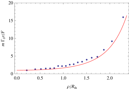
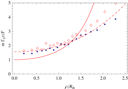
Figure 2: Color online. Transverse velocity field $v_{s}(\rho)$ in units of $m\Gamma_{0}/F$ in the infinitely elongated trap. Top: hydrodynamic regime, $\Gamma_{0}/\omega_{\perp}\simeq 100$; Bottom: collisionless regime $\Gamma_{0}/\omega_{\perp}\simeq 2$. The blue dots are simulation results for the constant scattering cross-section and the red solid line is the prediction $v_{s}(\rho)=F_{s}/m\Gamma(n_{0}(\rho))$ for the hydrodynamic regime. On the lower graph, the empty red diamonds are simulation results for the momentum dependent cross-section at $k_{\rm th}a=2$ and the red-dashed line represents the velocity field of a Maxwellian gas in the collisionless limit (see Supplemental Material).

Before solving this equation to find $\gamma$, we need to know the expression of the spin conductance $G$. We first consider the simpler case of a uniform gas of density $n_{+}=n_{-}=n_{0}=$ const. Using the method of moments Vichi and Stringari (1999), the velocity is solution of the equation $\partial_{t}v_{s}+\Gamma(n_{0})v_{s}=F_{s}/m$, where the spin damping rate $\Gamma$ is given by

$$\Gamma(n_{0})=\frac{1}{n_{0}}\int d^{3}\bm{p}f_{0}^{\rm(H)}(\bm{p})p_{z}C[p_{z}],$$ (4)

where $f_{0}^{\rm(H)}(\bm{p})=n_{0}e^{-p^{2}/2mk_{B}T}/(2\pi mk_{B}T)^{3/2}$ is the Gaussian phase-space density of a homogeneous gas and $C[\alpha]$ is the linearized collisional operator defined by

$$C[\alpha](\bm{p}_{1})=\int d^{3}\bm{p}_{2}f_{0}^{\rm(H)}(\bm{p}_{2})v_{\rm rel}\sigma(v_{\rm rel})\left(\alpha_{2}-\alpha_{1}\right),$$ (5)

where $v_{\rm rel}=|\bm{p}_{2}-\bm{p}_{1}|/m$, $\sigma$ is the s-wave scattering cross-section and $\alpha_{i}$ stands for $\alpha(\bm{p}_{i})$ . Generally speaking, $\Gamma$ is proportional to the collision rate, with a numerical prefactor depending on the actual form of the scattering cross-section. In the homogeneous case the stationary velocity is simply given by $v_{s}=F_{s}/m\Gamma(n_{0})$. In a trap, the density profile is inhomogeneous, which leads to a shear of the velocity field and a competition between viscosity and spin drag. Let $R_{\rm th}=\sqrt{k_{B}T/m\omega_{\perp}^{2}}$ be the transverse size of the cloud and $\nu$ its kinematic viscosity. Viscosity can be neglected as long as the viscous damping rate $\nu/R_{\rm th}^{2}$ is smaller than $\Gamma(n_{0})$. Since viscosity scales like $v_{\rm th}^{2}/\gamma_{\rm coll}$, with the thermal velocity $v_{\rm th}=\sqrt{k_{B}T/m}$, this condition is fulfilled as long as $\Gamma\propto\gamma_{\rm coll}\gg\omega_{\perp}$, in other words when the cloud is hydrodynamic in the transverse direction. In this regime we can therefore neglect viscous stress and the local velocity $v_{s}(\bm{\rho})=\int d^{3}\bm{p}f_{s}(\bm{\rho},\bm{p})v_{z}/n_{s}(\bm{\rho})$ is simply given by $v_{s}(\bm{\rho})=F_{s}/m\Gamma(n_{0}(\bm{\rho}))$, where $n_{0}(\rho)=n_{0}(0)\exp(-\rho^{2}/2R_{\rm th}^{2})$ is the local equilibrium density of the cloud.

This scaling for the velocity field is however too simple. Indeed, we have $\Phi_{s}=\int d^{2}\bm{\rho}n_{0}(\bm{\rho})v_{s}(\bm{\rho})\propto\int d^{2}\bm{\rho}n_{0}/\Gamma(n_{0}(\bm{\rho}))$, and since $\Gamma\propto n_{0}$, the integral is divergent. This pathology is cured by noting that the hydrodynamic assumption is not valid in the wings of the distribution where the density, and therefore the collision rate, vanish. The breakdown of the hydrodynamic approximation occurs when $\Gamma(n_{0}(\rho))\lesssim\omega_{\perp}$, i.e. when $\rho\gtrsim\rho_{\rm max}=R_{\rm th}\sqrt{2\ln(\Gamma_{0}/\omega_{\perp})}$, with $\Gamma_{0}=\Gamma(n_{0}(0))$ the local spin damping at the trap center. Considering $\rho_{\rm max}$ as a cut-off in the integral for $G$ we see that $G\simeq 2\pi\rho_{\rm max}^{2}n_{0}(0)/m\Gamma_{0}\propto\ln(\Gamma_{0})/\Gamma_{0}$.

In the opposite regime, when the gas is collisionless in the transverse direction, we expect viscous effects to flatten the velocity profile. Assuming a perfectly flat velocity field, then $v_{s}\propto F_{s}/m\Gamma_{0}$ and thus $G=\Phi_{s}/F_{s}\propto\bar{n}_{0}/m\Gamma_{0}$.

To make this scaling argument more quantitative, we calculate $G$ for different physical situations. First we calculate it numerically using the Boltzmann equation simulation described in Goulko et al. (2011, 2012). We initialise the axially homogeneous system at thermal equilibrium and then switch on the constant pulling force at $t=0$. We observe that in a few collision times, the total spin current of the cloud defined by $\Phi_{s}(t)=\langle v_{z}\rangle_{s}=\int d^{3}\bm{r}d^{3}\bm{p}f_{s}(\bm{r},\bm{p},t)v_{z}$ converges to a constant asymptotic value from which we extract the spin conductance $G(\bar{n}_{0})$. Figure 1 shows our results for the spin conductance for a constant cross section $\sigma=4\pi a^{2}$ and a momentum-dependent cross section $\sigma=4\pi a^{2}/(1+p_{\rm rel}^{2}a^{2}/4)$ near the unitary limit . When $G/n_{0}(0)$ is plotted versus $\Gamma_{0}=\Gamma(n_{0}(0))$ the data points overlap, showing that the drag coefficient depends only weakly on the actual momentum dependence of the scattering cross-section. To interpolate between the constant and the unitary cross section we also study the Maxwellian cross section $\sigma\propto 1/p$ for which we could find a semi-analytical expression of the spin conductance (see Supplemental Material).

Using these approaches, we find the following asymptotic behaviors. As expected, in the (transverse) collisionless limit $\Gamma_{0}\ll\omega_{\perp}$ the spin drag coefficient scales like $G\simeq kn_{0}(0)R_{\rm th}^{2}/m\Gamma_{0}$, where $k\simeq 16$ is a numerical coefficient, the value of which depends on the momentum dependence of the scattering cross-section (see Table 1). In the case of a Maxwellian gas, we find that $k=15.87$ (see Supplemental Material). For more general cases, a variational lower bound based on the exact Maxwellian solution yields an estimate very close to the numerical result obtained from the molecular dynamics simulation. In the opposite (hydrodynamic) limit $\Gamma_{0}\rightarrow\infty$, we recover the expected behavior $G\simeq 2\pi n_{0}(0)R_{\rm th}^{2}\ln(\Gamma_{0}/\omega_{\perp})/m\Gamma_{0}$.

$n$	$0$	$-1$	$-2$
Variational lower bound	14.5	15.87	17
Molecular dynamics	15.4	-	18.9

Table 1: Values of $k$ for a scattering cross-section $\sigma(p)\propto p^{n}$ for a constant cross-section ($n=0$), a Maxwellian gas ($n=-1$), and a unitary gas $(n=-2)$. For the Maxwellian gas, the lower bound is actually the exact result.

We also calculate the transverse velocity profile $v_{s}(\bm{\rho})$ and confirm that it obeys the expected behavior, see Fig. 2. For $\Gamma_{0}/\omega_{\perp}\gg 1$, we recover the viscousless prediction $v_{s}\propto 1/\Gamma(n_{0}(\bm{\rho}))$ while for $\Gamma_{0}\lesssim\omega_{\perp}$ we obtain a flatter velocity profile as a result of the transverse shearing. We see that in both regimes the velocity profile is not flat, and this explains the discrepancy between experiment and previous theoretical models based on uniform velocities.

Let us now return to the case of a three-dimensional trap and to the determination of the spin damping rate $\gamma$. According to Eq. (17) $\gamma$ appears as an eigenvalue of the operator $\widehat{S}=k_{B}T\bar{n}_{0}^{-1}\partial_{z}\left(G(z)\partial_{z}\cdot\right)$. This operator is hermitian on the Hilbert space of functions having a finite limit and zero derivative at $z=\pm\infty$ and since at long times the decay is dominated by the slowest mode, we focus on its smallest eigenvalue. We first consider the collisionless limit. In this regime, $G\propto n_{0}/\Gamma_{0}$ is position independent and can be considered as constant. Using the shooting method Press et al. (2007) we then obtain

$$\gamma\simeq 1.342\frac{k\omega_{z}^{2}}{2\pi\Gamma_{0}}.$$ (6)

where the value of $k$ is given in Table 1. For arbitrary values of $\Gamma_{0}/\omega_{\perp}$, we solve Eq. (17) using for $G$ a Padé interpolation of the simulation results presented in Fig. 1 (see Supplemental Material). Following Sommer et al. (2011a), we take $\Gamma_{\rm SD}=\omega_{z}^{2}/\gamma$ and in Fig. 3a we plot $\Gamma_{\rm SD}/\omega_{\perp}$ vs. $\Gamma_{0}/\omega_{\perp}$. We compare our model to the experimental results of Ref. Sommer et al. (2011a) and to a direct molecular dynamics simulation of the Boltzmann equation Goulko et al. (2011). In this simulation, the atoms are prepared in a harmonic trap of axial frequency $\omega_{\perp}=8\omega_{z}$. We displace their centers of mass by a distance $\pm z_{0}$, where $z_{0}$ is much smaller than the axial size of the cloud, and we fit the relative displacement vs time to an exponential from which we extract $\Gamma_{\rm SD}$. The results of these simulations are displayed in Fig. 3a where they are compared to the solutions of Eq. (17). We observe that the two approaches coincide both for the constant and momentum-dependent cross-sections .

As observed in Fig. 3b, theory and experiment agree remarkably as long as $T/T_{\rm F}\gtrsim 2$. Beyond that limit, we enter the quantum degenerate regime where the Boltzmann equation is no longer valid and, as expected, we observe that experiment and theory deviate from each other. In the high-temperature, collisionless limit, we find for the “unitary” value $k=18.9$, $\Gamma_{\rm SD}\simeq\Gamma_{0}/4.03$. This result differs from the high-temperature value $\Gamma_{\rm SD}\simeq\Gamma_{0}/5.7$ found in Sommer et al. (2011a). We interpret this discrepancy by noting that the theoretical asymptotic behavior Eq. (6) is valid for $\Gamma_{0}/\omega_{\perp}\lesssim 5$, while the experimental value was obtained by linear-fitting the points with $\Gamma_{0}/\omega_{\perp}\lesssim 15$, i.e. in a regime where the gas was likely less collisionless. Fitting our data on the same scale using a linear law would indeed give $\Gamma_{\rm SD}\simeq\Gamma_{0}/5.0$. We also note that our scaling $\Gamma_{\rm SD}=\omega_{\perp}f(\Gamma_{0}/\omega_{\perp})$ contradicts the scaling $\hbar\Gamma_{\rm SD}=E_{F}g(T/T_{F})$, where $E_{F}$ and $T_{F}$ are the Fermi energy and temperature, used in Ref. Sommer et al. (2011a) to analyze the experimental data. The two scalings agree only in the collisionless limit where $f$ is linear, hence outside of the region explored by experiments.

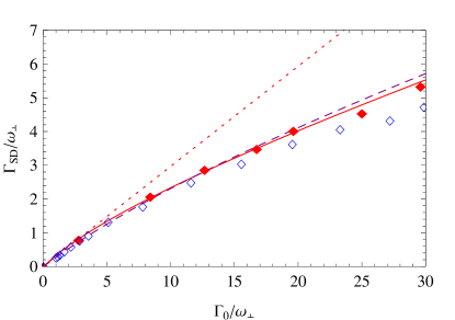
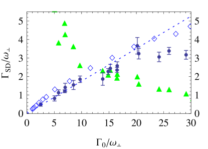
Figure 3: (Color online). Spin-drag coefficient $\Gamma_{\rm SD}$ in a harmonic trap. Top: theoretical predictions. For a constant cross-section the red solid diamonds are the results of the molecular dynamics simulation and the red solid line is the numerical resolution of the eigenequation (17). For a momentum dependent cross-section close to the unitary limit ($k_{\rm th}a=2$, with $k_{\rm th}=\sqrt{k_{B}T/\hbar^{2}}$ the thermal wave-vector), the blue open diamonds correspond to the molecular dynamics simulation while the the blue dashed line is the solution of Eq. (17). The red dotted line is the collisionless prediction $\Gamma_{\rm SD}=\Gamma_{0}/4.03$ for a unitary gas. Bottom: comparison with the experimental results of Ref. Sommer et al. (2011a) at unitarity (blue dots). The green triangles represent the associated values of $T/T_{\rm F}$. As above, the blue open diamonds correspond to the molecular dynamic simulation at $k_{\rm th}a=2$. Blue-dotted line: experimental fit $\Gamma_{\rm SD}\simeq\Gamma_{0}/5.7$. For the experimental data, $\Gamma_{0}$ is calculated using the theoretical value Eq. (4) for the unitary gas.

In summary, we have studied the classical dynamics of spin transport in a trap using the Boltzmann equation approach. By taking into account ab initio the trap inhomogeneity we are able to reproduce the experimental results without uncontrolled approximations and obtain several robust results which allow for a more rigorous extraction of transport coefficients from measurements in trapped cold gases. We highlight the competition between viscosity and spin drag in the shape of the velocity profile which is a crucial ingredient in the understanding of transport properties in a trap. We also demonstrate the breakdown of the universal scaling used to interpret the data of Ref. Sommer et al. (2011a) in the experimentally relevant range of parameters. In the future we anticipate extending this approach to lower temperatures where many-body interactions and Pauli blocking play a significant role.

We thank M. Zwierlein and A. Sommer for fruitful discussions and for providing us with the experimental data of Fig. 3. OG acknowledges support from the Excellence Cluster “Nanosystems Initiative Munich (NIM)”. FC acknowledges support from ERC (Advanced grant Ferlodim and Starting grant Thermodynamix), Région Ile de France (IFRAF) and Institut Universitaire de France. CL acknowledges support from EPSRC through grant EP/I018514.

I Supplemental Material to Spin Drag of a Fermi Gas in a Harmonic Trap

II Derivation of the transport equation from Boltzmann’s equation

We consider an ensemble of spin 1/2 fermions of mass $m$. In the dilute limit, the statistical properties of the system are fully captured by the single-particle phase-space densities $f_{s}(\bm{r},\bm{p},t)$ of the spin species $s=\pm$. In the presence of a trapping potential $V$, the evolution of $f_{s}$ is given by Boltzmann’s equation

$$\partial_{t}f_{s}+\frac{\bm{p}}{m}\cdot\partial_{\bm{r}}f_{s}+\bm{F}\cdot\partial_{\bm{p}}f_{s}=I_{\rm coll}[f_{s},f_{-s}],$$ (7)

where $\bm{F}=-\partial_{\bm{r}}V$ is the trapping force and $I_{\rm coll}$ is the collision operator. For low-temperature fermions, collisions between same-spin particles are suppressed and at low phase-space densities, the collision operator is given by

$$\begin{split}&I_{\rm coll}[f_{s},f_{-s}](\bm{r},\bm{p}_{1})=\\ &\int d^{3}\bm{p}_{2}d^{2}\bm{\Omega}^{\prime}v_{\rm rel}\frac{d\sigma}{d\Omega^{\prime}}\left(f_{s,3}f_{-s,4}-f_{s,1}f_{-s,2}\right),\end{split}$$ (8)

where $\bm{p}_{1}$ and $\bm{p}_{2}$ ($\bm{p}_{3}$ and $\bm{p}_{4}$) are ingoing (outgoing) momenta satisfying energy and momentum conservation, $v_{\rm rel}=|\bm{p}_{2}-\bm{p}_{1}|/m$ is the relative velocity, $d\sigma/d\Omega^{\prime}$ is the differential cross-section towards the solid angle $\bm{\Omega}^{\prime}$ and $f_{s,i}$ stands for $f_{s}(\bm{r},\bm{p}_{i})$.

When the populations of the two spin states are equal, the equilibrium solution of Eq. (7) is given by the Maxwell-Boltzmann distribution $f_{+}=f_{-}=f_{0}={\cal A}\exp\left[-\beta(p^{2}/2m+V)\right]$, where $\beta=1/k_{B}T$ and ${\cal A}$ is an integration constant such that $\int d^{3}\bm{r}d^{3}\bm{p}f_{0}$ is the population of one spin state. We consider a spin perturbation of the form $f_{s}(\bm{r},\bm{p},t)=f_{0}(\bm{r},\bm{p})\left(1+s\alpha(\bm{r},\bm{p},t)\right)$. Assuming the perturbation is small enough, we can expand Boltzmann’s equation in $\alpha$ and to first order we obtain

$$\partial_{t}\alpha+\frac{\bm{p}}{m}\cdot\partial_{\bm{r}}\alpha+\bm{F}\cdot\partial_{\bm{p}}\alpha=-C[\alpha],$$ (9)

where, for s-wave collisions, the linearized collisional operator $C$ is given by

$$C[\alpha](\bm{r},\bm{p}_{1})=\int d^{3}\bm{p}_{2}f_{0}(\bm{r},\bm{p}_{2})v_{\rm rel}\sigma(v_{\rm rel})\left(\alpha_{1}-\alpha_{2}\right),$$ (10)

and as above $\alpha_{i}=\alpha(\bm{r},\bm{p}_{i})$. In experiments, the trap can be described by a cylindrically-symmetric harmonic potential with frequency $\omega_{z}$ along the symmetry axis $z$ and $\omega_{\perp}$ in the transverse $(x,y)$ plane. In the rest of this Supplemental Material, we work in a unit system where $m=k_{B}T=\omega_{\perp}=1$ and we then write $V(x,y,z)=(\omega_{z}^{2}z^{2}+\rho^{2})/2$, with $\bm{\rho}=(x,y)$.

We look for exponentially decaying solutions corresponding to small deviations from equilibrium, and therefore take $\alpha(\bm{r},\bm{p},t)=e^{-\gamma t}\widetilde{\alpha}(\bm{r},\bm{p})$. Eq. (9) then becomes

$$\left[-\gamma+p_{z}\partial_{z}-\omega_{z}^{2}z\partial_{p_{z}}\right]\widetilde{\alpha}=-\left[\bm{\Pi}\cdot\partial_{\bm{\rho}}-\bm{\rho}\cdot\partial_{\bm{\Pi}}+C\right]\widetilde{\alpha},$$ (11)

where $\bm{\Pi}=(p_{x},p_{y})$ is the projection of the momentum in the $(x,y)$ plane. We note that in the rhs of Eq. (11) the only $z$-dependence is in the linearized collisional operator $C$, from $f_{0}\propto\exp(-\omega_{z}^{2}z^{2}/2)$. Let $C=\bar{n}_{0}(z)\tilde{C}$, where $\bar{n}_{0}(z)=\int d^{2}\bm{\rho}d^{3}\bm{p}f_{0}(\bm{r},\bm{p})=\bar{n}_{0}(0)e^{-\omega_{z}^{2}z^{2}/2}$ is the equilibrium 1D-density and $\tilde{C}$ no longer acts on the coordinate $z$. Taking $z^{\prime}=\omega_{z}z$, we obtain

$$\left[-\gamma+\omega_{z}(p_{z}\partial_{z^{\prime}}-z^{\prime}\partial_{p_{z}})\right]\widetilde{\alpha}=-{\cal L}_{\bar{n}_{0}(z^{\prime})}[\widetilde{\alpha}],$$ (12)

with

$${\cal L}_{\bar{n}_{0}(z^{\prime})}=\bar{n}_{0}(z^{\prime})\tilde{C}+\bm{\Pi}\cdot\partial_{\bm{\rho}}-\bm{\rho}\cdot\partial_{\bm{\Pi}}.$$ (13)

Note that ${\cal L}_{\bar{n}_{0}(z^{\prime})}$ depends on the axial coordinate $z^{\prime}$ only through the axial density. In particular, $z^{\prime}$ is only a parameter of the operator since we neither integrate nor differentiate with respect to this coordinate.

Two properties of ${\cal L}_{\bar{n}}$ will be used below: (i) its kernel is spanned by the functions of $z^{\prime}$ only and (ii) due to atom number conservation, we have for any $\widetilde{\alpha}$, $\int d^{2}\bm{\rho}d^{3}\bm{p}f_{0}{\cal L}_{\bar{n}}[\widetilde{\alpha}]=0$. We look for solutions of Eq. (12) in the limit of a very elongated trap $\omega_{z}\rightarrow 0$. If we focus on the slow axial spin dynamics of the cloud studied experimentally in Sommer et al. (2011a), we have also $\gamma\rightarrow 0$ and we can therefore expand $\gamma$ and $\widetilde{\alpha}$ as $\gamma=\sum_{n\geq 1}\gamma_{n}\omega_{z}^{n}$ and $\widetilde{\alpha}(\bm{r},\bm{p})=\sum_{n\geq 0}\omega_{z}^{n}a_{n}(\bm{r},\bm{p})$. Note that we are ultimately interested in the coefficient $\gamma_{2}$, since we take $\Gamma_{\rm SD}=\omega_{z}^{2}/\gamma$ as in Sommer et al. (2011a). Inserting these expansions in Eq. (12) we get to zero-th order ${\cal L}_{\bar{n}}[a_{0}]=0$ . According to property (i), $a_{0}$ is thus a function of $z^{\prime}$ only. It is determined explicitly by the study of the next order terms of the expansion. For $n=1$ we obtain

$$-\gamma_{1}a_{0}+p_{z}\partial_{z^{\prime}}a_{0}=-{\cal L}_{\bar{n}_{0}(z^{\prime})}[a_{1}].$$ (14)

Using property (ii), we see readily that $\gamma_{1}=0$, which then leads to the following relation:

$$p_{z}\partial_{z^{\prime}}a_{0}=-{\cal L}_{\bar{n}_{0}(z^{\prime})}[a_{1}].$$ (15)

Consider a uniform density $\bar{n}$ and assume for a moment that we know the solution $\chi_{\bar{n}}(\bm{\rho},\bm{p})$ of the integro-differential equation $p_{z}={\cal L}_{\bar{n}}[\chi_{\bar{n}}]$ (the properties of $\chi_{\bar{n}}$ will be discussed below). Since $\bar{n}_{0}(z^{\prime})$ is only a parameter, and by linearity of $\cal L$, the solution of Eq. (15) is thus $a_{1}=-\chi_{\bar{n}_{0}(z^{\prime})}\partial_{z^{\prime}}a_{0}$.

Having expressed $a_{1}$ as a function of $a_{0}$, we close the set of equations by considering the $n=2$ term of the expansion. It reads:

$$\left(-\gamma_{2}a_{0}+(p_{z}\partial_{z^{\prime}}-z^{\prime}\partial_{p_{z}})a_{1}\right)=-{\cal L}_{\bar{n}_{0}(z^{\prime})}[a_{2}].$$ (16)

Using the expression of $a_{1}$ as well as the property (ii), we obtain after integration by parts

$$\gamma_{2}\bar{n}_{0}(z^{\prime})a_{0}(z^{\prime})+\partial_{z^{\prime}}\left(G(z^{\prime})\partial_{z^{\prime}}a_{0}(z^{\prime})\right)=0,$$ (17)

where

$$G(z^{\prime})\equiv\int d^{2}\bm{\rho}d^{3}\bm{p}f_{0}p_{z}\chi_{\bar{n}_{0}(z^{\prime})}(\bm{\rho},\bm{p}).$$ (18)

We now show that $G$ defined above can be identified with the spin conductance of an ideal gas of 1D density $\bar{n}$ in a cylindrical harmonic trap. Indeed, by definition, the conductance is obtained by solving Boltzmann’s equation in a cylindrical trap in the presence of a spin pulling force $\bm{F}_{s}=sF_{0}\bm{e}_{z}$. Expanding Eq. (7) to first order in perturbation, and taking as above $f_{s}=f_{0}(1+s\alpha(\bm{\rho},\bm{p}))$, we see that $\alpha$ is solution of

$$F_{0}p_{z}={\cal L}_{\bar{n}}[\alpha].$$ (19)

We recognize here the same equation as for the definition of $\chi$ and we then have $\alpha=F_{0}\chi_{\tilde{n}}$. Since the particle flux is given by $\Phi=\int d^{3}\bm{p}d^{2}\bm{\rho}f_{0}\alpha p_{z}$, we see finally that, as claimed above, $G=\Phi/F_{0}=\int d^{2}\rho d^{3}\bm{p}f_{0}p_{z}\chi_{\tilde{n}}(\bm{\rho},\bm{p})$.

III Spin drag coefficient for the Maxwellian gas

Consider the special case of the radially trapped Maxwellian gas for which $\sigma(p)=\Lambda/p$ where $\Lambda$ is some constant. This model is useful to interpolate between the weakly interacting ($\sigma=$const.) and the strongly interacting ($\sigma\propto 1/p^{2}$) limits. Taking the ansatz $\alpha(\bm{r},\bm{p})=F_{0}p_{z}H(\bm{\rho},\bm{\Pi})/2$, Boltzmann’s equation for spin excitations turns into

$$\frac{1}{2}\left(\bm{\Pi}\cdot\partial_{\bm{\rho}}-\bm{\rho}\cdot\partial_{\bm{\Pi}}\right)H(\bm{\rho},\bm{\Pi})-1=-\frac{\Gamma_{0}}{2}e^{-\rho^{2}/2}H(\bm{\rho},\bm{\Pi}),$$ (20)

with $\Gamma_{0}=\Lambda n_{0}$ the damping rate of the spin excitations of a homogeneous gas of density $n_{0}$. Using the rotational invariance around the $z$ axis, the phase space density can be expressed using the new variables

$$h = (\Pi^{2}+\rho^{2})/2$$

$$u = (\Pi^{2}-\rho^{2})/2$$

$$v = \bm{\Pi}\cdot\bm{\rho}.$$

Let $u+iv=Re^{i\varphi}$. Eq. (20) then becomes

$$\partial_{\varphi}H(h,R,\varphi)-1=-\frac{\Gamma_{0}e^{-h/2}}{2}e^{R\cos\varphi/2}H(h,R,\varphi).$$ (21)

Moreover, in these new variables, we have

$$\int d^{2}\bm{\Pi}d^{2}\bm{\rho}\cdots=2\pi\int_{h=0}^{\infty}\int_{x=0}^{1}\int_{\varphi=0}^{2\pi}\frac{xdx\,hdh\,d\varphi}{\sqrt{1-x^{2}}}\cdots.$$ (22)

where $R=xh$ and the dots stand for any cylindrically symmetric function of $\bm{\Pi}$ and $\bm{\rho}$. In particular, the spin-conductance is given by

$$G=\frac{n_{0}}{2}\int\frac{xdx\,hdh\,d\varphi}{\sqrt{1-x^{2}}}e^{-h}H(h,R=xh,\varphi),$$ (23)

We now turn to the solution of Eq. (21) where we focus on the $\varphi$-dependence, since it is the only variable appearing in the differential operator. Eq. (21) takes the general form

$$H^{\prime}(\varphi)+\mu A(\varphi)H(\varphi)=1,$$ (24)

with $\mu=\Gamma_{0}e^{-h/2}/2$ and $A=\exp(R\cos(\varphi)/2)$ is a $2\pi$-periodic function. Take

$$K_{\mu}(\varphi)=\exp\left[-\mu\int_{0}^{\varphi}d\varphi^{\prime}A(\varphi^{\prime})\right],$$ (25)

the general solution of (24) is

$$H(\varphi)=K_{\mu}(\varphi)\int_{\varphi_{0}}^{\varphi}\frac{d\varphi^{\prime}}{K_{\mu}(\varphi^{\prime})},$$ (26)

where $\varphi_{0}$ is an integration constant that can be determined by imposing the periodicity of $H$. Taking $H(0)=H(2\pi)$, we have finally

$$H(\varphi)=K_{\mu}(\varphi)\left[\int_{0}^{\varphi}\frac{d\varphi^{\prime}}{K_{\mu}(\varphi^{\prime})}+\frac{K_{\mu}(2\pi)}{1-K_{\mu}(2\pi)}\int_{0}^{2\pi}\frac{d\varphi^{\prime}}{K_{\mu}(\varphi^{\prime})}\right].$$ (27)

Let’s now discuss the behavior of the solutions in the collisionless and hydrodynamic limits.

III.1 Collisionless limit $\mu\rightarrow 0$

In this limit, $K_{\mu}\simeq 1-\mu\int_{0}^{\varphi}A(\varphi^{\prime})d\varphi^{\prime}$. The asymptotic behavior of $H$ is then dominated by the singularity due to the denominator $1-K_{\mu}(2\pi)$ that vanishes for $\mu=0$. To leading order, we see that $H$ does not depend on $\varphi$ and is given by

$$H=\frac{1}{\mu\bar{A}},$$ (28)

where

$$\bar{A}=\frac{1}{2\pi}\int_{0}^{2\pi}A(\varphi^{\prime})d\varphi^{\prime}=I_{0}(R/2)$$ (29)

is the average value of $A$ ($I_{0}$ is the zeroth-order modified Bessel function of the first kind).

Using the actual values of $\mu$ and $A$ we have

$$G \sim \frac{n_{0}}{\Gamma_{0}}\int_{h=0}^{\infty}\int_{x=0}^{1}\frac{hdh\,xdx}{\sqrt{1-x^{2}}}\frac{2\pi e^{-h/2}}{{\rm I}_{0}(xh/2)}$$ (30)

$$\sim \frac{15.87}{\Lambda},$$ (31)

Note in particular that $G$ does not depend on the density of the cloud.

Within this limit the velocity field in the collisionless regime is given by

$$v(\rho)=\frac{F_{0}}{2\pi\Gamma_{0}}\int\frac{e^{(\rho^{2}-\Pi^{2})/4}\Pi d\Pi d\theta}{I_{0}\left(\frac{1}{2}\sqrt{\Pi^{2}\rho^{2}\cos^{2}\theta+(\Pi^{2}-\rho^{2})^{2}/4}\right)}$$ (32)

III.2 Hydrodynamic limit $\mu\rightarrow\infty$

In the limit $\Gamma_{0}\rightarrow\infty$ we may neglect the transport term $H^{\prime}$ in (24), yielding $H(\varphi)=1/\mu A(\varphi)\propto 1/\Gamma_{0}$. Taking $\Gamma(\bm{\rho})=\Gamma_{0}e^{-\rho^{2}/2}$, the local spin damping rate, we recover the expected result $v(\rho)\propto 1/\Gamma(\bm{\rho})$, that was obtained in the main text using local density arguments.

IV A variational result for the collisionless spin conductance

The spin conductance in a transverse trap is obtained by solving the linearized Boltzmann equation

$$\left(\bm{\Pi}\cdot\partial_{\bm{\rho}}-\bm{\rho}\cdot\partial_{\bm{\Pi}}\right)\alpha-Fp_{z}=-C[\alpha],$$ (33)

where $C$ is the linearized collisional operator defined by

$$C[\alpha](\bm{\rho},\bm{p}_{1})=\int d^{3}\bm{p}_{2}f_{0}(\bm{\rho},\bm{p}_{2})|\bm{p}_{2}-\bm{p}_{1}|\sigma\left[\alpha(\bm{\rho},\bm{p}_{1})-\alpha(\bm{\rho},\bm{p}_{2})\right].$$ (34)

We recall that $C$ is symmetric and positive for the scalar product

$$\langle g_{1}|g_{2}\rangle=\int d^{2}\bm{\rho}d^{3}\bm{p}g_{1}(\bm{\rho},\bm{p})g_{2}(\bm{\rho},\bm{p})f_{0}(\bm{\rho},\bm{p}),$$ (35)

where $f_{0}(\bm{\rho},\bm{p})=n_{0}e^{-(p^{2}+\rho^{2})/2}/\sqrt{2\pi}^{3}$ is the static phase-space density, and $n_{0}$ is the density at the center of the trap.

The spin current is defined by $\Phi=\int d^{3}\bm{p}d^{2}\bm{\rho}f_{0}\alpha p_{z}=\langle\alpha|p_{z}\rangle$ and the spin conductance is then $G=\Phi/F$. Letting $\alpha(\bm{\rho},\bm{p})=Fa(\bm{\rho},\bm{p})$ we have more simply $G=\langle p_{z}|a\rangle$.

We work in the collisionless limit $\sigma\rightarrow 0$ and we thus take $\sigma(p_{\rm rel})=\varepsilon\hat{\sigma}(p_{\rm rel})$ and $C=\varepsilon C_{2}$ where $\varepsilon$ is small. Following the results obtained for the Maxwellian gas, we expand $a$ as

$$a(\bm{\rho},\bm{p})=\frac{a_{0}(\bm{\rho},\bm{p})}{\varepsilon}+a_{1}(\bm{\rho},\bm{p})+\varepsilon a_{2}(\bm{\rho},\bm{p})+\ldots$$ (36)

Inserting this expansion in Boltzmann’s equation, we obtain to leading order

$$\left(\bm{\Pi}\cdot\partial_{\bm{\rho}}-\bm{\rho}\cdot\partial_{\bm{\Pi}}\right)a_{0}=0.$$ (37)

This equation is solved readily by introducing the variables $(p_{z},h,x,\varphi)$ defined in the study of the Maxwellian gas.

In these coordinates, Eq. (37) becomes simply $\partial_{\varphi}a_{0}=0$. The set ${\cal F}_{0}$ of solutions of Eq. (37) is thus composed of functions whose value does not depend on the angle $\varphi$. To get the actual expression of $a_{0}$ we need to go one step further in the expansion. At this order in $\varepsilon$, we have

$$\partial_{\varphi}a_{1}-p_{z}=-C_{2}[a_{0}].$$ (38)

To get rid of $a_{1}$, we integrate over $\varphi$ and use the fact that the $a_{n}$ are periodic functions of $\varphi$. We then obtain the equation

$$\bar{C}_{2}[a_{0}]=p_{z},$$ (39)

with $\bar{C}_{2}[a_{0}]=\int d\varphi C_{2}[a_{0}]/2\pi$ and where $a_{0}$ is now the only unknown.

We define on ${\cal F}_{0}$ the new scalar product

$$(a|b)=4\pi^{2}\int\frac{xdx\,hdh\,dp_{z}}{\sqrt{1-x^{2}}}f_{0}a(x,h,p_{z})b(x,h,p_{z}),$$ (40)

which is equivalent to the old scalar product $\langle a|b\rangle$. We then see readily that $(a|\bar{C}[b])=\langle a|C[b]\rangle$. Using the properties of $C$, we deduce that $\bar{C}_{2}$ is a symmetric, positive operator on ${\cal F}_{0}$. Eq. (39) then has the same structure as the ones used to calculate transport coefficients in homogeneous systems. We can then use the usual tricks to get a bound on the spin conductance Smith and Jensen (1989). We indeed write that for any real $\lambda$ and any function $b\in{\cal F}_{0}$, we have $(a_{0}+\lambda b|\bar{C}_{2}[a_{0}+\lambda b])\geq 0$, and using the fact that this second order polynomial in $\lambda$ is always positive, we obtain from the negativity of the discriminant that for any $b$,

$$G\geq\frac{(p_{z}|b)^{2}}{(b|\bar{C}[b])}=\frac{\langle p_{z}|b\rangle^{2}}{\langle b|C[b]\rangle},$$ (41)

the bound being reached for $b=a_{0}$. We take as a variational ansatz $b=p_{z}$, since as discussed earlier, the collisionless regime is associated with a rather flat velocity profile. We then obtain

$$G\geq\frac{\left(\int d^{2}\bm{\rho}e^{-\rho^{2}/2}\right)^{2}}{\int d^{2}\bm{\rho}e^{-\rho^{2}}}\frac{n_{0}}{\Gamma_{0}}=4\pi\frac{n_{0}}{\Gamma_{0}},$$ (42)

with $\Gamma_{0}$ the spin drag on the axis of the trap. The prefactor is $4\pi\simeq 12.56$, not far from the result 15.87 found analytically for the Maxwellian gas, and the bound is indeed satisfied.

An improved variational bound can be obtained by using the exact result Eq. (32) found for the Maxwellian gas to estimate the spin drag for constant-momentum or unitary-limited cross-sections. For the Maxwellian gas, this gives by definition the exact result, while for the constant cross-section and the unitary gases, we obtain respectively $\Gamma\geq 14.5/\Gamma_{0}$ and $\Gamma\geq 17/\Gamma_{0}$.

V Interpolation scheme for the spin conductance

We know that for a power-law cross-section , the spin conductance $G$ scales like $n_{0}(0)/\Gamma_{0}f(1/\Gamma_{0})$ where $f$ obeys the following asymptotic behaviors:

1. In the collisionless limit, $f$ converges to a constant value ($\simeq 15.87$ for the Maxwellian gas).

2. In the hydrodynamic limit, $f$ has a logarithmic singularity and scales like $2\pi\ln\Gamma_{0}$.

To interpolate between these two limits we make use of the Bessel function $K_{0}$ which vanishes at $+\infty$ and diverges as $-\ln x$ at $x=0$. We thus approximate $f$ by

$$f(x)=2\pi K_{0}(x)+15.87\frac{x+a}{x+b},$$ (43)

where $a$ and $b$ are determined by fitting the results of the molecular dynamics simulations (see Fig. 4). In the case of a constant cross-section, we obtain $a=0.11$ and $b=0.52$. We note that the largest relative error between the Padé interpolation and the result of the molecular simulation is observed for the largest values of $\Gamma_{0}$ and amounts to $\simeq 6$ % for $\Gamma_{0}\simeq 10$.

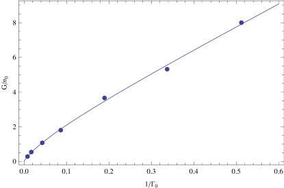
Figure 4: Spin conductance $G$ for a constant cross-section. Dots: Molecular Dynamics Simulation. Solid line: Padé’s approximation.

References

- Zwerger (2012) W. Zwerger, ed., The BCS-BEC Crossover and the Unitary Fermi Gas, vol. 836 of Lecture Notes in Physics (Springer, Berlin, 2012).
- Brantut et al. (2012) J.-P. Brantut, J. Meineke, D. Stadler, S. Krinner, and T. Esslinger, Science 337, 1069 (2012).
- Cao et al. (2011) C. Cao, E. Elliott, J. Joseph, H. Wu, J. Petricka, T. Schäfer, and J. E. Thomas, Science 331, 58 (2011), ISSN 0036-8075.
- Kovtun et al. (2005) P. Kovtun, D. T. Son, and A. Starinets, Phys. Rev. Lett. 94, 111601 (2005).
- Liao et al. (2011) Y. Liao, M. Revelle, T. Paprotta, A. Rittner, W. Li, G. Partridge, and R. Hulet, Phys. Rev. Lett. 107, 145305 (2011).
- Bruun (2012) G. Bruun, Phys. Rev. A 85, 013636 (2012).
- Enss and Haussmann (2012) T. Enss and R. Haussmann, Phys. Rev. Lett. 109, 195303 (2012).
- Wong et al. (2012) C. Wong, H. Stoof, and R. Duine, Phys. Rev. A 85, 063613 (2012).
- Heiselberg (2012) H. Heiselberg, Phys. Rev. Lett. 108, 245303 (2012).
- Kittinaradorn et al. (2012) R. Kittinaradorn, R. Duine, and H. Stoof, New Journal of Physics 14, 055007 (2012).
- Kim and Huse (2012) H. Kim and D. A. Huse, Phys. Rev. A 86, 053607 (2012).
- Musaelian and Meyerovich (1992) K. Musaelian and A. Meyerovich, Journal of Low Temperature Physics 89, 535 (1992), ISSN 0022-2291, URL http://dx.doi.org/10.1007/BF00694081.
- Mineev (2004) V. P. Mineev, Phys. Rev. B 69, 144429 (2004), URL http://link.aps.org/doi/10.1103/PhysRevB.69.144429.
- Wolf et al. (2001) S. Wolf, D. Awschalom, R. Buhrman, J. Daughton, S. Von Molnar, M. Roukes, A. Y. Chtchelkanova, and D. Treger, Science 294, 1488 (2001).
- Sommer et al. (2011a) A. Sommer, M. Ku, G. Roati, and M. W. Zwierlein, Nature 472, 201 (2011a).
- Sommer et al. (2011b) A. Sommer, M. Ku, and M. W. Zwierlein, New Journal of Physics 13, 055009 (2011b).
- Bruun and Pethick (2011) G. Bruun and C. Pethick, Phys. Rev. Lett. 107, 255302 (2011).
- Vichi and Stringari (1999) L. Vichi and S. Stringari, Phys. Rev. A 60, 4734 (1999).
- Chiacchiera et al. (2010) S. Chiacchiera, T. Macri, and A. Trombettoni, Phys. Rev. A 81, 033624 (2010).
- Bruun (2011) G. M. Bruun, New Journal of Physics 13, 035005 (2011).
- Goulko et al. (2011) O. Goulko, F. Chevy, and C. Lobo, Phys. Rev. A 84, 051605 (2011).
- Goulko et al. (2012) O. Goulko, F. Chevy, and C. Lobo, New Journal of Physics 14, 073036 (2012).
- Press et al. (2007) W. H. Press, S. A. Teukolsky, W. T. Vetterling, and B. P. Flannery, Numerical recipes 3rd edition: The art of scientific computing (Cambridge university press, 2007).
- Smith and Jensen (1989) H. Smith and H. H. Jensen, Transport phenomena (Oxford University Press, USA, 1989).

References

- Zwerger (2012) W. Zwerger, ed., The BCS-BEC Crossover and the Unitary Fermi Gas, vol. 836 of Lecture Notes in Physics (Springer, Berlin, 2012).
- Brantut et al. (2012) J.-P. Brantut, J. Meineke, D. Stadler, S. Krinner, and T. Esslinger, Science 337, 1069 (2012).
- Cao et al. (2011) C. Cao, E. Elliott, J. Joseph, H. Wu, J. Petricka, T. Schäfer, and J. E. Thomas, Science 331, 58 (2011), ISSN 0036-8075.
- Kovtun et al. (2005) P. Kovtun, D. T. Son, and A. Starinets, Phys. Rev. Lett. 94, 111601 (2005).
- Liao et al. (2011) Y. Liao, M. Revelle, T. Paprotta, A. Rittner, W. Li, G. Partridge, and R. Hulet, Phys. Rev. Lett. 107, 145305 (2011).
- Bruun (2012) G. Bruun, Phys. Rev. A 85, 013636 (2012).
- Enss and Haussmann (2012) T. Enss and R. Haussmann, Phys. Rev. Lett. 109, 195303 (2012).
- Wong et al. (2012) C. Wong, H. Stoof, and R. Duine, Phys. Rev. A 85, 063613 (2012).
- Heiselberg (2012) H. Heiselberg, Phys. Rev. Lett. 108, 245303 (2012).
- Kittinaradorn et al. (2012) R. Kittinaradorn, R. Duine, and H. Stoof, New Journal of Physics 14, 055007 (2012).
- Kim and Huse (2012) H. Kim and D. A. Huse, Phys. Rev. A 86, 053607 (2012).
- Musaelian and Meyerovich (1992) K. Musaelian and A. Meyerovich, Journal of Low Temperature Physics 89, 535 (1992), ISSN 0022-2291, URL http://dx.doi.org/10.1007/BF00694081.
- Mineev (2004) V. P. Mineev, Phys. Rev. B 69, 144429 (2004), URL http://link.aps.org/doi/10.1103/PhysRevB.69.144429.
- Wolf et al. (2001) S. Wolf, D. Awschalom, R. Buhrman, J. Daughton, S. Von Molnar, M. Roukes, A. Y. Chtchelkanova, and D. Treger, Science 294, 1488 (2001).
- Sommer et al. (2011a) A. Sommer, M. Ku, G. Roati, and M. W. Zwierlein, Nature 472, 201 (2011a).
- Sommer et al. (2011b) A. Sommer, M. Ku, and M. W. Zwierlein, New Journal of Physics 13, 055009 (2011b).
- Bruun and Pethick (2011) G. Bruun and C. Pethick, Phys. Rev. Lett. 107, 255302 (2011).
- Vichi and Stringari (1999) L. Vichi and S. Stringari, Phys. Rev. A 60, 4734 (1999).
- Chiacchiera et al. (2010) S. Chiacchiera, T. Macri, and A. Trombettoni, Phys. Rev. A 81, 033624 (2010).
- Bruun (2011) G. M. Bruun, New Journal of Physics 13, 035005 (2011).
- Goulko et al. (2011) O. Goulko, F. Chevy, and C. Lobo, Phys. Rev. A 84, 051605 (2011).
- Goulko et al. (2012) O. Goulko, F. Chevy, and C. Lobo, New Journal of Physics 14, 073036 (2012).
- Press et al. (2007) W. H. Press, S. A. Teukolsky, W. T. Vetterling, and B. P. Flannery, Numerical recipes 3rd edition: The art of scientific computing (Cambridge university press, 2007).
- Smith and Jensen (1989) H. Smith and H. H. Jensen, Transport phenomena (Oxford University Press, USA, 1989).