Faraday and Cotton-Mouton Effects of Helium at $\lambda=1064$ nm

Abstract

We present measurements of the Faraday and the Cotton-Mouton effects of helium gas at $\lambda~{}=~{}1064$ nm. Our apparatus is based on an up-to-date resonant optical cavity coupled to longitudinal and transverse magnetic fields. This cavity increases the signal to be measured by more than a factor of 270 000 compared to the one acquired after a single path of light in the magnetic field region. We have reached a precision of a few percent both for Faraday effect and Cotton-Mouton effect. Our measurements give for the first time the experimental value of the Faraday effect at $\lambda$= 1064 nm. This value is compatible with the theoretical prediction. Concerning Cotton-Mouton effect, our measurement is the second reported experimental value at this wavelength, and the first to agree at better than 1$\sigma$ with theoretical predictions.

I Introduction

In 1845 Faraday discovered that a magnetic field affects the propagation of light in a medium Faraday1846 . In particular, he observed that a magnetic field parallel to the light wave vector k induces a polarization rotation of a linearly polarized light. This effect is known nowadays as the Faraday effect. With such experiments, Faraday was looking for the proof that light and magnetic field have a common origin. These revolutionary findings have been one of the most important steps towards Maxwell’s theory of electromagnetism.

At the very beginning of the 20th century, Kerr Kerr and Majorana Majorana discovered that a linearly polarized light, propagating in a medium in the presence of a magnetic field, also acquires an ellipticity when the field is perpendicular to k. In the following years, this phenomenon has been studied in details by A. Cotton and H. Mouton CottonMouton and it is known nowadays as the Cotton-Mouton effect.

Faraday and Cotton-Mouton effects are both due to the fact that the magnetic field creates an anisotropy in the medium which then becomes birefringent. The term birefringent indicates that different states of polarization do not have the same propagation velocity. The Faraday effect corresponds to a magnetic circular birefringence, i.e. the index of refraction $n_{-}$ for left circularly polarized light is different from the index of refraction $n_{+}$ for right circularly polarized light. The difference $\Delta n_{\mathrm{F}}=n_{-}-n_{+}$ is proportional to the longitudinal magnetic field $B_{\|}$:

$$\Delta n_{\mathrm{F}}=k_{\mathrm{F}}B_{\|},$$ (1)

where $k_{\mathrm{F}}$ is the circular magnetic birefringence per Tesla. On the other hand, the Cotton-Mouton effect corresponds to a magnetic linear birefringence, $i.e.$ the index of refraction $n_{\parallel}$ for light polarized parallel to the magnetic field is different from the index of refraction $n_{\perp}$ for light polarized perpendicular to the magnetic field. The difference $\Delta n_{\mathrm{CM}}=n_{\parallel}-n_{\perp}$ is proportional to the square of the transverse magnetic field $B_{\bot}^{2}$:

$$\Delta n_{\mathrm{CM}}=k_{\mathrm{CM}}B_{\bot}^{2},$$ (2)

where $k_{\mathrm{CM}}$ is the linear magnetic birefringence per Tesla squared.

Such magnetic birefringences are usually very small ($\Delta n_{\mathrm{F}},\Delta n_{\mathrm{CM}}\ll 1$) for magnetic fields available in laboratories, especially in the case of dilute matter. Magnetic birefringence measurements are therefore an experimental challenge. The value of the birefringence depends on the microscopic matter response properties like (hyper)susceptibilities. In the case of dilute matter, these responses can be calculated ab initio using the computational methods developed in the framework of quantum chemistry Rizzo2005 . Experimental measurements are then a fundamental test of our knowledge of the interaction of electromagnetic fields and matter.

Among all known gases, helium presents the smallest Faraday and Cotton-Mouton effects. Ab initio calculations of the helium Faraday effect at $\lambda=1064$ nm, with $\lambda$ the light wavelength, have been published only recently Ekstrom2005 . From the experimental point of view, even if Faraday effect measurements in helium dates back to the 50s Ingersoll1956 , no measurement has yet been reported at $\lambda=1064$ nm. Helium Cotton-Mouton effect has been first measured at $\lambda=514.5$ nm in 1991 Cameron1991 . At the same time, the first numerical calculation at a different wavelength in the coupled Hartree-Fock approximation was published Jamieson . Actually, these two first values were not in agreement. While some other theoretical calculations exist in literature Rizzo1997 , only three more experimental values have been published since 1991 Cameron1991 ; Muroo2003 ; Bregant2009 , with only one at $\lambda=1064$ nm Bregant2009 .

Ab initio calculations of both Faraday and Cotton-Mouton effect of helium are benchmark tests for computational methods. In practice they can be considered as error free, especially when compared with the error bars associated with the experimental values. Experimental measurement precision has therefore to be as good as possible to be able to test the different computational methods.

Experimentally, one generally measures the Faraday effect by measuring the polarization rotation angle $\theta_{\mathrm{F}}$, related to the circular birefringence by the formula:

$$\theta_{\mathrm{F}}=\pi\frac{L_{B}}{\lambda}\Delta n_{\mathrm{F}},$$ (3)

where $L_{B}$ is the length of the magnetic field region. The Cotton-Mouton effect is measured through the induced ellipticity related to the linear birefringence by the formula:

$$\psi=\pi\frac{L_{B}}{\lambda}\Delta n_{\mathrm{CM}}\sin 2\theta_{\mathrm{P}},$$ (4)

where $\theta_{\mathrm{P}}$ is the angle between light polarization and the magnetic field. Experiments are difficult because one needs a high magnetic field coupled to optics designed to detect very small variations of light velocity. One also needs a $L_{B}$ as large as possible. To this end, optical cavities are used to trap light in the magnetic field region and therefore increase the ellipticity to be measured (see e.g. Ref. Cameron1991 ).

In this paper, we present measurements of the Faraday and the Cotton-Mouton effects of helium gas at $\lambda=1064$ nm. Our apparatus is based on an up-to-date resonant optical cavity coupled to longitudinal and transverse magnetic fields. This cavity increases the signal to be measured by more than a factor of 270 000 compared to the one acquired after a single path of light in the magnetic field region. This allows us to reach a measurement precision of a few percent both for Faraday effect and Cotton-Mouton effect. Our results are finally compared to the theoretical predictions and they agree to within better than 1$\sigma$.

II Experimental setup and signal analysis

II.1 Apparatus

Our apparatus is described in details in Refs. Berceau2012 ; Battesti2008 . Briefly, as shown in Fig. 1, 30 mW linearly polarized light provided by a Nd:YAG laser ($\lambda=1064$ nm) is injected into a high finesse Fabry-Pérot cavity consisting of the mirrors M₁ and M₂. The laser frequency is locked onto the cavity using the Pound-Drever-Hall method Drever1983 . To this end, the laser passes through an electro-optic modulator (EOM) creating sidebands at 10 MHz. The beam reflected by the cavity is detected by the photodiode Ph_r. This signal is used to adjust the laser frequency with a bandwidth of 80 kHz thanks to an acousto-optic modulator (AOM) and with a bandwidth of a few kHz thanks to the piezoelectric element of the laser. A slow control with a bandwidth of a few mHz is also applied thanks to the Peltier element of the laser.

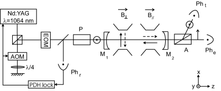
Figure 1: Experimental setup. EOM = electro-optic modulator; AOM = acousto-optic modulator; PDH = Pound-Drever-Hall; Ph = photodiode; P = polarizer; A = analyzer. See text for more details.

Before entering the optical cavity, the light is linearly polarized by the polarizer P. The light transmitted by the cavity is then analyzed with the analyzer A crossed at maximum extinction. Both polarizations are extracted: parallel and perpendicular to P. The extraordinary beam (power $I_{\mathrm{e}}$), corresponding to the light polarization perpendicular to P, is collected by the low noise photodiode Ph_e, while the ordinary beam (power $I_{\mathrm{t}}$), corresponding to the light polarization parallel to P, is detected by Ph_t. All the optical components from the polarizer P to the analyzer A are placed in a high vacuum chamber which can be filled with high purity gases. During this work, magneto-optical measurements have been done using a bottle of helium gas with a global purity higher than 99.9999 $\%$. This bottle is connected to the chamber through a leak valve allowing to inject less than $10^{-3}$ atm of gas.

Magnets providing a field perpendicular to the light wave vector k and a field parallel to k surround the vacuum pipe. The transverse magnetic field ($\textbf{B}_{\perp}\perp\textbf{k}$) used for Cotton-Mouton effect measurements is created thanks to pulsed coils described in Refs. Battesti2008 ; Batut2008 and briefly detailed in section IV.1. For the Faraday effect measurements, a modulated longitudinal magnetic field ($\textbf{B}_{\parallel}\parallel\textbf{k}$) is applied thanks to a solenoid. More details are given in section III.1.

II.2 Fabry-Pérot cavity

A key element of the experiment is the Fabry-Pérot cavity. Its aim is to accumulate the effect of the magnetic field by trapping the light between two ultra high reflectivity mirrors M₁ and M₂. The length of the cavity is $L_{\mathrm{c}}=(2.2713\pm 0.0006)$ m. This corresponds to a cavity free spectral range of $\Delta^{\mathrm{FSR}}=c/2nL_{\mathrm{c}}=(65.996\pm 0.017)$ MHz, with $c$ the speed of light in vacuum and $n$ the index of refraction of the medium in which the cavity is immersed. This index of refraction will be considered equal to one. All theses parameters and their uncertainties were measured previously. Details concerning the measurement are given in Ref. Berceau2012 . Using the Jones matrix formalism, we can calculate the total acquired ellipticity due to the Cotton-Mouton effect $\Psi(t)$. It is linked to the ellipticity without any cavity $\psi(t)$ by:

$$\Psi(t)=\frac{2F}{\pi}\psi(t),$$ (5)

Likewise, the total rotation angle $\Theta_{\mathrm{F}}(t)$ due to the Faraday effect is:

$$\Theta_{\mathrm{F}}(t)=\frac{2F}{\pi}\theta_{\mathrm{F}}(t).$$ (6)

where $F$ is the finesse of the cavity and $\theta_{\mathrm{F}}(t)$ the rotation angle without any cavity.

II.2.1 Cavity birefringence

The cavity induces a total static ellipticity $\Gamma$. This is due to the mirrors intrinsic phase retardation Bielsa2009 . Each mirror can be regarded as a wave plate and combination of both wave plates gives a single wave plate. The total phase retardation $\delta_{\mathrm{eq}}$ and the axis orientation of the wave plate equivalent to the cavity depend on the phase retardation of each mirror and on their relative orientation Brandi1997 ; Jacob1995 . Thus the value of $\Gamma$ can be adjusted by rotating the mirrors M₁ and M₂ around the $z$-axis corresponding to the axis of light propagation.

We first set $\Gamma=0$. To this end, we align the axis of the equivalent wave plate on the incident polarization. This is done by rotating the mirrors while the laser frequency is locked onto the cavity. As the polarizers are crossed at maximum extinction, we can measure the extinction ratio $\sigma^{2}$ of the polarizers by measuring the following ratio:

$$\sigma^{2}=\frac{I_{\mathrm{e}}}{I_{\mathrm{t}}}\Big{|}_{\Gamma=0}.$$ (7)

The value of $\sigma^{2}$ is regularly measured, in particular before each shot for the Cotton-Mouton effect measurements. This extinction ratio can typically vary from $4\times 10^{-7}$ to $8\times 10^{-7}$.

As shown in Ref. Battesti2008 , because of the ellipticity noise, the optical sensitivity improves when $\Gamma$ decreases. Starting from $\Gamma=0$ and rotating M₁ in the clockwise or counterclockwise direction, we choose the sign of $\Gamma$ as well as its value, with typically $\Gamma^{2}\sim\sigma^{2}$. The sign of $\Gamma$ is known by filling the vacuum chamber with nitrogen gas and by measuring its Cotton-Mouton effect, whose sign and value are perfectly known. This measurement has already been done with this experiment and results are reported in Ref. Berceau2012 . We performed several measurements with different signs and values of $\Gamma$, showing that this parameter is perfectly controlled. The value and the sign of $\Gamma$ are set before each magnetic shot.

The static birefringence of the cavity changes the incident linear polarization into an elliptical polarization of ellipticity $\Gamma$. But it also induces a rotation angle $\epsilon$ of the major axis of the ellipse compared with the P polarizer axis. The value of this angle can be calculated considering the Fabry-Pérot cavity as an equivalent wave plate of phase retardation $\delta_{\mathrm{eq}}$. The angle between the incident linear polarization and the fast axis of the equivalent wave plate corresponds to $\varphi$, as represented in Fig. 2. The ellipticity induced by the wave plate is given by:

$$\Gamma=\frac{\sin(2\varphi)\sin(\delta_{\mathrm{eq}})}{2}.$$ (8)

As we set $\Gamma\ll 1$, the fast axis is almost aligned with $P$ and thus, we have $\varphi\ll 1$. Assuming that $\delta_{\mathrm{eq}}\ll 1$, we get:

$$\varphi=\frac{\Gamma}{\delta_{\mathrm{eq}}}.$$ (9)

We also have:

$$\tan(2\theta) = \tan(2\varphi)\cos(\delta_{\mathrm{eq}}),$$ (10)

$$\theta = \varphi\Big{(}1-\frac{\delta_{\mathrm{eq}}^{2}}{2}\Big{)},$$ (11)

where $\theta$ is the angle between the major axis of the ellipse and the fast axis of the wave plate. Combining Eqs. (9) and (11), we obtain the angle $\epsilon$ between the major axis of the elliptical polarization and the incident linear polarization:

$$\epsilon=\theta-\varphi=-\frac{\Gamma\delta_{\mathrm{eq}}}{2}.$$ (12)

The value of the phase retardation of our cavity is about $|\delta_{\mathrm{eq}}|\sim 0.1$ rad. This has been inferred by measuring the value of $\Gamma$ as a function of the mirrors’ orientation, as explained in details in Ref. Bielsa2009 . With a typical value of $|\Gamma|$ varying from $8\times 10^{-4}$ to $3\times 10^{-3}$, we obtain $40~{}\mu\mathrm{rad}<|\epsilon|<150~{}\mu$rad.

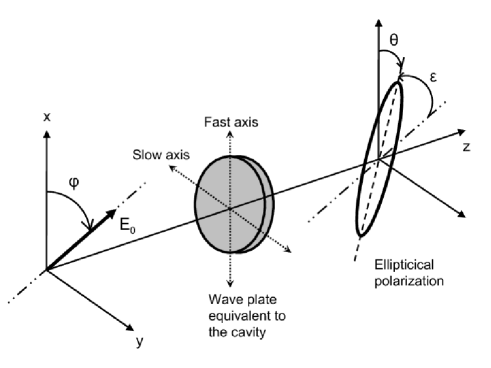
Figure 2: Rotation of the major axis of the elliptical polarization due to the static birefringence of the Fabry-Pérot cavity.

II.2.2 Cavity finesse and cavity filtering

The finesse of the cavity is inferred from the measurement of the photon lifetime $\tau$ inside the cavity. At $t=t_{0}$ the intensity of the laser, previously locked onto the cavity resonance, is switched off. The exponential decay of the intensity of the ordinary beam for $t>t_{0}$ is fitted with:

$$I_{\mathrm{t}}(t)=I_{\mathrm{t}}(t_{\mathrm{0}})e^{-(t-t_{\mathrm{0}})/\tau},$$ (13)

to obtain $\tau$. The cavity finesse is related to the photon lifetime through:

$$F=\frac{\pi c\tau}{L_{\mathrm{c}}}.$$ (14)

The value of the photon lifetime is regularly checked during data taking. In this experiment, it ranges from 1.06 ms to 1.12 ms, corresponding to a finesse of 438 000 to 465 000. During a run of data taking, the relative variation of the photon lifetime does not exceed 2$\%$ at 1$\sigma$ confidence level.

Due to the photon lifetime, the cavity acts as a first order low pass filter, as explained in details in Ref. Berceau2010 . Its complex response function $H(\nu)$ is given by:

$$H(\nu)=\frac{1}{1+i\frac{\nu}{\nu_{\mathrm{c}}}},$$ (15)

with $\nu$ the frequency and $\nu_{\mathrm{c}}=1/4\pi\tau\simeq 70$ Hz the cavity cutoff frequency. This filtering has to be taken into account in particular for the time dependent magnetic field applied inside the Fabry-Pérot cavity.

The cavity also acts as a first order low pass filter for the ordinary beam $I_{\mathrm{t}}(t)$ compared to the beam incident on the cavity. But, due to the cavity birefringence, the cavity acts as a second order low pass filter for the extraordinary beam $I_{\mathrm{e}}(t)$. This effect is explained in details in Ref. Berceau2010 . The second order low pass filter represents the combined action of two successive identical first order low pass filters. Their complex response function is given by Eq. (15). While the first one characterizes the usual cavity behavior, we can interpret the second filter in terms of pumping or filling: due to the mirror birefringence, some photons of the ordinary beam are gradually converted into the extraordinary beam at each reflection. Thus, if we want to directly compare $I_{\mathrm{t}}(t)$ and $I_{\mathrm{e}}(t)$, one has to apply the first order low pass filter to $I_{\mathrm{t}}(t)$. The filtered signal $I_{\mathrm{t,f}}(t)$ is then used for the analysis.

II.3 Signals

The ellipticity $\Psi(t)$ and the rotation of the polarization $\Theta_{\mathrm{F}}(t)$ induced by the transverse and the longitudinal magnetic fields can be related to the ratio of the extraordinary and ordinary powers as follows:

$$\frac{I_{\mathrm{e}}(t)}{I_{\mathrm{t,f}}(t)}=\sigma^{2}+[\Gamma+\Psi(t)]^{2}+[\epsilon+\Theta_{\mathrm{F}}(t)]^{2}.$$ (16)

This formula, which can be obtained using the Jones formalism, clearly shows that our experiment is sensitive to both ellipticities and rotations.

III Faraday effect of helium gas

As stated above, the Faraday effect corresponds to a magnetic circular birefringence $\Delta n_{\mathrm{F}}$ induced by a longitudinal magnetic field $B_{\|}$. Form Eqs. (1), (3) and (6), we deduce that the polarization rotation to be measured depends on $k_{\mathrm{F}}$ as follows:

$$\Theta_{\mathrm{F}}(t)=2F\frac{L_{B}}{\lambda}k_{\mathrm{F}}{B_{\|}}(t).$$ (17)

For historical reasons, Faraday effect is usually given in terms of the Verdet constant $V$ Verdet1854 , that is related to the Faraday constant as:

$$V=\frac{\pi k_{\mathrm{F}}}{\lambda}.$$ (18)

Eq. (17) becomes:

$$\Theta_{\mathrm{F}}(t)=\frac{2F}{\pi}VB_{\|}(t)L_{B}.$$ (19)

III.1 Magnetic field

To measure the Faraday effect, we need a longitudinal magnetic field. It is delivered thanks to a 300 mm long solenoid. Its diameter is 50 mm and it corresponds to 340 loops of copper wire. The magnetic field profile along the longitudinal $z$-axis has been measured with a gaussmeter. Fig. 3 shows the normalized profile. We define $B_{\|,0}$ as the maximum magnetic field, thus at the center of the coil, and $L_{B}$ as the equivalent magnetic length such that:

$$\int^{+\infty}_{-\infty}B_{\|}(z)dz\equiv B_{\|,0}L_{B}.$$ (20)

This equivalent magnetic length has been calculated by numerically integrating the measured field. Taking into account the experimental uncertainties, we obtain $L_{B}=(0.308\pm 0.006)$ m at 1$\sigma$. We can reach a maximum magnetic field of about $4.3$ mT corresponding to an injected current of 3 A.

Figure 3: Normalized profile of the longitudinal magnetic field inside the solenoid along the longitudinal $z$-axis. The crosses correspond to the measurements.

To measure the magnetic field during operation, we measure the current injected into the coil. The form factor $B_{\|}/I$ has been determined experimentally using the gaussemeter and an ammeter. This form factor remains constant for frequency modulation ranging from DC to 50 Hz. Finally we have estimated the relative uncertainty $u(B_{\|})/B_{\|}=1.4\%$ at 1$\sigma$, taking into account the uncertainties coming from the gaussmeter, the ammeter and from a possible small misalignment of the laser beam inside the solenoid.

Faraday effect measurements were performed at room temperature $T=293$ K in an air-conditioned room. When a current is injected into the solenoid, the temperature increases inside the coil. Nevertheless, for a maximum current of 3 A, the increase is lower than 2 K. This will be taken into account in the final uncertainty.

III.2 Analysis of Faraday signal

The magnetic field at the center of the coil is modulated at the frequency $\nu$: $B_{\|}=B_{\|,0}\sin(2\pi\nu t+\phi)$. The rotation of the polarization due to the Faraday effect is thus given by:

$$\Theta_{\mathrm{F}} = \Theta_{0}\sin(2\pi\nu t+\phi),$$ (21)

$$\mathrm{with}\;\Theta_{0} = \frac{2F}{\pi}VB_{\|,0}L_{B}.$$ (22)

Expanding Eq. (16), we obtain:

$$\frac{I_{\mathrm{e}}(t)}{I_{\mathrm{t,f}}(t)}=\sigma^{2}+\epsilon^{2}+2\epsilon\Theta_{\mathrm{F}}(t)+\Theta_{\mathrm{F}}^{2}(t)+\Gamma^{2}+2\Gamma\Psi(t)+\Psi^{2}(t).$$ (23)

We define the ratio between the Faraday and the Cotton-Mouton signals as:

$$R_{\mathrm{F/CM}}=\frac{2\epsilon\Theta_{\mathrm{F}}+\Theta_{\mathrm{F}}^{2}}{2\Gamma\Psi+\Psi^{2}}.$$ (24)

For the Faraday measurements, our typical static ellipticity is $\Gamma=3\times 10^{-3}$ rad, and Eq. (12) gives $|\epsilon|=150\,\mu$rad. We evaluate the value of $R_{\mathrm{F/CM}}$ using the theoretical values of the Verdet and Cotton-Mouton constants of helium which are given later in this article. For this experiment, our typical helium pressure is $30\times 10^{-3}$ atm and the cavity finesse is of the order of 465 000 corresponding to a cavity cutoff frequency of about 70 Hz. The solenoid mainly induces a longitudinal magnetic field, but, for the sake of argument, let’s perform the calculation with the same value 4.3 mT for the longitudinal and the transverse magnetic field. One gets: $R_{\mathrm{F/CM}}\sim 10^{6}$. The Cotton-Mouton effect is thus negligible. Eq. (23) thus becomes:

$$\frac{I_{\mathrm{e}}(t)}{I_{\mathrm{t,f}}(t)}=\sigma^{2}+\Gamma^{2}+[\epsilon+\Theta_{\mathrm{F}}(t)]^{2}.$$ (25)

This equation results in three main frequency components:

$$I_{\mathrm{DC}} = \sigma^{2}+\Gamma^{2}+\epsilon^{2}+\frac{\Theta_{0}^{2}}{2},$$ (26)

$$I_{\mathrm{\nu}} = \frac{2\epsilon\Theta_{0}}{\sqrt{1+\big{(}\frac{\nu}{\nu_{\mathrm{c}}}\big{)}^{2}}}\sin\Big{[}2\pi\nu t+\phi-\arctan\Big{(}\frac{\nu}{\nu_{\mathrm{c}}}\Big{)}\Big{]},$$ (27)

$$I_{\mathrm{2\nu}} = -\frac{\Theta_{0}^{2}}{2\sqrt{1+\big{(}\frac{2\nu}{\nu_{\mathrm{c}}}\big{)}^{2}}}\cos\Big{[}4\pi\nu t+2\phi-\arctan\Big{(}\frac{2\nu}{\nu_{\mathrm{c}}}\Big{)}\Big{]}.$$

As mentionned before, the cavity acts as a first-order low-pass filter, with a cavity cutoff frequency $\nu_{\mathrm{c}}$. This filtering has been taken into account in Eqs. (27) and (LABEL:Eq:Faraday_2f).

The amplitude of the $\nu$-component, $I_{\nu}$ depends on $\Theta_{0}$ but also on $\epsilon$ whose value is not precisely known. On the other hand, $I_{\mathrm{2\nu}}$ only depends on $\Theta_{0}$. Consequently it is the only component used to measure the Verdet constant. The amplitude of the $2\nu$ frequency component, proportional to $(B_{\|,0}L_{B})^{2}$, is measured as a function of the magnetic field amplitude. We fit our data by $K_{V}B_{\|,0}^{2}$. The Verdet constant $V$ finally depends on the measured experimental parameters as follows, using Eq. (22) and the amplitude of the $2\nu$-component given in Eq.(LABEL:Eq:Faraday_2f):

$$V(T,P)=\sqrt{\frac{K_{V}}{2}}\frac{\Big{[}1+{(8\pi\tau\nu)}^{2}\Big{]}^{1/4}}{2\tau\Delta^{\mathrm{FSR}}L_{B}}.$$ (29)

III.3 Results

III.3.1 Our result

We report in Fig. 4 the Fourier transform of $I_{\mathrm{e}}/I_{\mathrm{t,f}}-DC$-signal with about $60\times 10^{-3}$  atm of helium and with $B_{\|,0}L_{B}=1.3\times 10^{-3}$ Tm. The magnetic frequency modulation is fixed to $\nu=18$ Hz in order to have the $2\nu$ frequency lower than the cavity cutoff frequency. We can observe both components at frequencies $\nu$ and $2\nu$. During the Faraday data taking, the photon lifetime was $\tau=(1.12\pm 0.02)$ ms corresponding to a cavity finesse of ($465\,000\pm 8\,000)$.

Figure 4: Fourier transform of $I_{\mathrm{e}}/I_{\mathrm{t}}-DC$ with about $60\times 10^{-3}$ atm of helium and with $B_{\|,0}L_{B}=1.3\times 10^{-3}$ T.m. The magnetic frequency modulation is $\nu=18$ Hz.

We plot in Fig. 5 the amplitude of the $2\nu$ component as a function of $B_{\|,0}$. We fit our data by a quadratic law $K_{V}B_{\|,0}^{2}$. We also study the $\nu$ frequency component as a function of the magnetic field amplitude. According to the relation (27), we obtain a linear dependance. By fitting these data by a linear equation and using the value of the Verdet constant measured with the $2\nu$ frequency component, we infer the value of the $\epsilon$ parameter. We obtain $\epsilon\simeq 10^{-4}$ rad, in agreement with the value calculated with Eq. (12).

Figure 5: Amplitude of the $2\nu$ frequency component as a fonction of $B_{\|,0}$ with about $60\times 10^{-3}$  atm of helium. The solid line corresponds to the quadratic fit of the experimental data.

We performed Faraday constant measurements at different pressures from $10^{-2}$ to $6\times 10^{-2}$ atm. They are summarized in Fig. 6. We measure the gas pressure in the chamber with pressure gauges which have a relative uncertainty given by the manufacturer of 0.2$\%$. In this range of pressure, helium can be considered as an ideal gas and the pressure dependence of the Verdet constant is thus linear. As shown in Fig. 6, our data are correctly fitted by a linear equation. Its $V$-axis intercept is consistent with zero within the uncertainties. Its slope gives the normalized Verdet constant at $\lambda=1064$ nm and at $T=(294\pm 1)$ K:

$$V=(3.87\pm 0.12)\times 10^{-5}\;\mathrm{atm}^{-1}\mathrm{rad.T}^{-1}\mathrm{m}^{-1}.$$ (30)

With a scale law on the gas density and considering an ideal gas, this corresponds to a normalized Verdet constant at $T=273.15$ K of:

$$V=(4.17\pm 0.13)\times 10^{-5}\;\mathrm{atm}^{-1}\mathrm{rad.T}^{-1}\mathrm{m}^{-1}.$$ (31)

The uncertainty is given at 1$\sigma$. It is calculated from the relative A and B-type uncertainties summarized in Table 1 and detailed in Ref. Berceau2012 . Using Eq. (18), we can also give the normalized Faraday constant. At $T=273.15$ K, one gets:

$$k_{\mathrm{F}}=(1.41\pm 0.04)\times 10^{-11}\;\mathrm{atm}^{-1}\mathrm{T}^{-1}.$$ (32)

Parameter	Relative A-type	Relative B-type
	uncertainty	uncertainty
$\tau$	$2\times 10^{-2}$
$K_{V}$	$8\times 10^{-3}$
$B_{\|,0}$		$1.4\times 10^{-2}$
$L_{B}$		$2.0\times 10^{-2}$
$\Delta^{\mathrm{FSR}}$		$3\times 10^{-4}$
$P$		$2\times 10^{-3}$

Table 1: Parameters and their respective relative A and B-type uncertainties at 1$\sigma$ that have to be measured to infer the value of the normalized Verdet constant $V$.

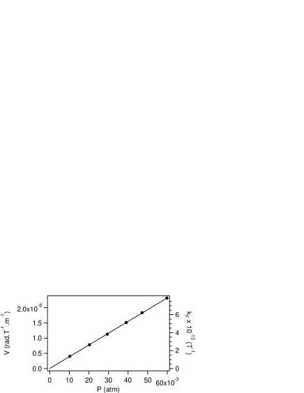
Figure 6: Verdet constant of helium as a function of pressure. The solid line corresponds to the linear fit of the experimental data.

III.3.2 Comparison

Our value of the normalized Verdet constant can be compared to other published values. Ref. Ingersoll1956 presents the most extensive experimental values in helium. They have been measured at different wavelengths, from 363 nm to 900 nm, and they correspond to the open triangles in Fig. 7 at $T=273.15$ K. As stated by the authors in Refs. Ingersoll1956 ; Ingersoll1954 , “the average absolute probable error is considered to be about 1$\%$”, but “the scale of measurement was determined by a comparison of these results with accepted values for water”. This is an important difference from our experiment since we do not need to calibrate our setup with another gas. All parameters from which the measured Verdet constant depends are accurately monitored, yielding therefore a Verdet constant of high precision and accuracy.

As far as we know, no value has been reported at 1064 nm, our working wavelength. Nevertheless, it can be quadratically interpolated from the data of Ref. Ingersoll1956 with a fit $A/\lambda^{2}$ (solid line in Fig. 7). This gives a normalized Verdet constant at $\lambda=1064$ nm and $T=273.15$ K of $V=(4.15\pm 0.05)\times 10^{-5}\,\mathrm{atm}^{-1}\mathrm{rad.T}^{-1}\mathrm{m}^{-1}$. The uncertainty is the one given by the fit. This value is compatible with ours, which is represented as the open circle in the inset of Fig. 7.

Figure 7: $\vartriangle$: Experimental values of helium normalized Verdet constant at $T=273.15$ K reported in Ref. Ingersoll1956 for wavelength from 363 nm to 900 nm. These values are fitted by the law $A/\lambda^{2}$ (solid line). $\circ$: Our experimental value at $T=273.15$ K. $\bullet$: Theoretical predictions at $T=273.15$ K reported in Ref. Ekstrom2005 . Inset : Zoom around $\lambda=1064$ nm. The error bar corresponds to the 1$\sigma$ uncertainty of our measurement.

We finally compared our value with the theoretical predictions at $T=273.15$ K. The most recent ones were published in 2005 Ekstrom2005 exploiting a four-component Hartree-Fock calculations and in 2012 Savukov2012 using a relativistic particle hole configuration interaction method. Ref. Ekstrom2005 gives values at different wavelengths that are plotted in Fig. 7 with the filled points. The value at $\lambda=1064$ nm is $V=4.06\times 10^{-5}\,\mathrm{atm}^{-1}\mathrm{rad.T}^{-1}\mathrm{m}^{-1}$ and it is plotted in Fig. 7 with the filled point. Ref. Savukov2012 does not give a value at 1064 nm, but it can be obtained by a quadratic interpolation the data provided by the authors. One obtains $V=(4.09\pm 0.02)\times 10^{-5}\,\mathrm{atm}^{-1}\mathrm{rad.T}^{-1}\mathrm{m}^{-1}$, with an uncertainty given by the fit. Both theoretical values are compatible with our experimental Verdet constant. All these theoretical and experimental values are summarized in Table 2.

Ref.	$V\times 10^{5}$	Remarks
	[$\mathrm{atm}^{-1}\mathrm{rad.T}^{-1}\mathrm{m}^{-1}$]
	Theoretical values
Ekstrom2005	4.06
Savukov2012	$4.09\pm 0.02$	quadratically interpolated
	Experimental values
Ingersoll1956	$4.15\pm 0.05$	quadratically interpolated
		not absolute: scaled to
		water
This work	$4.17\pm 0.13$

Table 2: Experimental and theoretical values of the normalized Verdet constant at $T=273.15$ K, $\lambda=1064$ nm and with uncertainties at 1$\sigma$.

IV Cotton-Mouton effect of helium gas

The Cotton-Mouton effect consists in a linear birefringence $\Delta n_{\mathrm{CM}}$ induced by a transverse magnetic field $B_{\perp}$. From Eqs. (4) and (5) we deduce that the ellipticity $\Psi(t)$ to be measured is linked to $k_{\mathrm{CM}}$ by:

$$\Psi(t) = 2F\frac{L_{B}}{\lambda}k_{\mathrm{CM}}B_{\perp}^{2}(t)\sin 2\theta_{\mathrm{P}}.$$ (33)

The angle $\theta_{\mathrm{P}}$ is adjusted to 45 degrees with the experimental procedure explained in Ref. Berceau2012 .

IV.1 Magnetic field

One can see that $\Psi$ is proportional to $B_{\perp}^{2}L_{B}$. In order to have $\Psi$ as high as possible, we have to maximize this parameter. This is fulfilled using pulsed fields delivered by one magnet, named X-coil, especially designed by the LNCMI. The principle of this magnet and its properties are described in details in Refs. Battesti2008 ; Batut2008 . It can provide a maximum field of more than 14T over an equivalent length $L_{B}$ of 0.137 m Berceau2012 . The high voltage connections can be remotely switched to reverse the direction of the field. Thus we can set B parallel or anti-parallel to the $x$-direction, as shown in Fig. 1.

The pulsed coil is immersed in a liquid nitrogen cryostat to limit its heating. A pause between two pulses is necessary to let the magnet cool down to the equilibrium temperature. We do not need to use the coil at its maximum field since the sensitivity of our experiment is largely sufficient. We have chosen to apply a maximum field of 3 T in order to limit the ageing of the magnet. From one shot to another, a relative variation of the maximum of the field lower than 1.5 $\%$ was observed due to a variation of the power supply voltage.

The pulse duration is less than 10 ms, with the maximum of the field reached within 2 ms. Since the pulse duration is of the same order of magnitude as the photon lifetime inside the cavity, the filtering of the Fabry-Pérot cavity has to be taken into account for the magnetic field, as said in section II.2.2. We calculate the filtered field $B^{2}_{\perp,\mathrm{f}}$ from $B_{\perp}^{2}$ by using the first-order low pass filter corresponding to the cavity. The time profiles of $B_{\perp}^{2}$ and $B^{2}_{\perp,\mathrm{f}}$ are shown in Fig. 8, for a maximum field of 3 T.

Figure 8: Square of the magnetic field amplitude as a function of time for a maximum field of 3 T. Solid black curve: $B_{\perp}^{2}$, dashed curve: $B^{2}_{\perp,\mathrm{f}}$.

IV.2 Analysis of Cotton-Mouton signal

As mentioned in section II.3, the ratio of power $I_{\mathrm{e}}$ and $I_{\mathrm{t,f}}$ is linked to the birefringence $\Psi(t)$ to be measured as follows:

$$\frac{I_{\mathrm{e}}(t)}{I_{\mathrm{t,f}}(t)}=\sigma^{2}+[\Gamma+\Psi(t)]^{2}+[\epsilon+\Theta_{\mathrm{F}}(t)]^{2},$$ (34)

where $\Theta_{\mathrm{F}}(t)$ is the rotation angle due to a longitudinal component of the pulsed magnetic field inducing a Faraday effect in helium. This component $B_{\parallel}(t)$ is firstly due to the X-structure of the coil. It is around 230 times smaller than the transverse field, $i.e.$ around 10 mT for a pulse of 3 T. Moreover a contribution to $B_{\parallel}$ appears if the cryostat is not perfectly aligned with the optical axis. The diameter of the cryostat is 60 cm. A typical misalignment of 2 mm over this length, i.e. around 3 mrad, leads to a longitudinal component of 10 mT. Finally the estimated longitudinal magnetic field is about 20 mT. It can be present during a shot over an equivalent length $L_{B}=0.137$ m.

Using Eq. (19) and the value of the Verdet constant given in Eq. (30), we can calculate the rotation of the polarization $\Theta_{\mathrm{F}}$ due to $B_{\parallel}$. It is about 30 mrad per atmosphere of helium gas. We then calculate the ratio of the Faraday effect over the Cotton-Mouton effect $R_{\mathrm{F/CM}}$, given by Eq. (24). Since the static ellipticity is typically $|\Gamma|\simeq 8\times 10^{-4}$ rad corresponding to $\epsilon\simeq 40\,\mu$rad as stated in section II.2.1, this ratio goes from 200 at $40\times 10^{-3}$ atm to 2600 at $550\times 10^{-3}$ atm. This shows that the Faraday effect component is not negligible and thus need to be taken into account.

From Eq. (34), we obtain:

$$\frac{I_{\mathrm{e}}(t)}{I_{\mathrm{t,f}}(t)}=\sigma^{2}+\Gamma^{2}+\epsilon^{2}+2\Gamma\Psi(t)+\Psi^{2}(t)+2\epsilon\Theta_{\mathrm{F}}(t)+\Theta_{\mathrm{F}}^{2}(t).$$ (35)

This formula shows that the angle $\epsilon$ carries the Faraday effect of the gas. During a Cotton-Mouton effect measurement we want to have the Faraday effect as small as possible. We therefore minimize $\epsilon$ before the shot, once the value of $\Gamma$ is set, by turning the analyzer A. As we can see in Fig. 2, it consists in aligning A, which has been initially adjusted at 90 degrees compared to the incident polarization, on the minor axis of the elliptical polarization. Nevertheless, in order to take into account the imperfections of this experimental adjustment, we still keep $\epsilon$ in the formula, assuming that $\epsilon^{2}\ll\Gamma^{2}$.

To extract the ellipticity $\Psi(t)$, we calculate the following $Y(t)$ function:

$$Y(t) = \frac{\frac{I_{\mathrm{e}}(t)}{I_{\mathrm{t,f}}(t)}-DC}{2|\Gamma|}$$

$$= \gamma\Psi(t)+\frac{\Psi^{2}(t)}{2|\Gamma|}+\gamma\frac{|\epsilon|\Theta_{\mathrm{F}}(t)}{2|\Gamma|}+\frac{\Theta_{\mathrm{F}}^{2}(t)}{2|\Gamma|},$$

where $\gamma$ corresponds to the sign of $\Gamma$. $DC$ is the static signal:

$$DC=\sigma^{2}+\Gamma^{2}+\epsilon^{2}=\Big{<}\frac{I_{\mathrm{e}}(t)}{I_{\mathrm{t,f}}(t)}\Big{>}_{t<0},$$ (37)

and it is measured just before each shot, the magnetic field being applied at $t=0$. We also measure the extinction ratio $\sigma^{2}$ before each shot using the experimental procedure described in section II.2.1. The absolute value of the static ellipticity is then calculated as follows:

$$|\Gamma|=\sqrt{\Big{<}\frac{I_{\mathrm{e}}(t)}{I_{\mathrm{t,f}}(t)}\Big{>}_{t<0}-\sigma^{2}}.$$ (38)

Two parameters are adjustable in the experiment: the sign $\gamma$ of the static ellipticity $\Gamma$ and the direction of the transverse magnetic field. We acquire signals for both signs of $\Gamma$ and both directions of B: parallel to $x$ is denoted as $>0$ and antiparallel is denoted as $<0$. This gives four data series: ($\Gamma>0$, $B_{\perp}>0$), ($\Gamma>0$, $B_{\perp}<0$), ($\Gamma<0$, $B_{\perp}<0$) and ($\Gamma<0$, $B_{\perp}>0$). For each series, signals calculated with Eq. (IV.2) are averaged and denoted as $Y_{>>}$, $Y_{><}$, $Y_{<<}$ and $Y_{<>}$. The first subscript corresponds to $\Gamma>0$ or $<0$ while the second one corresponds to B parallel or antiparallel to $x$.

The $Y$ signals are the sum of different effects with different symmetries, denoted as $S$:

$$Y_{>>} = a_{>>}S_{++}+b_{>>}S_{+-}+c_{>>}S_{--}+d_{>>}S_{-+},$$

$$Y_{><} = a_{><}S_{++}-b_{><}S_{+-}-c_{><}S_{--}+d_{><}S_{-+},$$

$$Y_{<<} = a_{<<}S_{++}-b_{<<}S_{+-}+c_{<<}S_{--}-d_{<<}S_{-+},$$

$$Y_{<>} = a_{<>}S_{++}+b_{<>}S_{+-}-c_{<>}S_{--}-d_{<>}S_{-+}.$$

The first subscript in $S$ corresponds to the symmetry towards the sign of $\Gamma$ and the second one towards the direction of B. The subscript $+$ indicates an even parity while the subscript $-$ indicates an odd parity. In practice $w_{>>}\simeq w_{><}\simeq w_{<<}\simeq w_{<>}$ (with $w=a,~{}b,~{}c$ or $d$) depend on the experimental parameters. These values are not perfectly equal because the experimental parameters slightly vary from one shot to another, in particular the value of $|\Gamma|$.

Possible physical effects contributing to the different $S$ signals are summarized in Tab. 3. The $S_{+-}$ signal does not appear in Eq. (IV.2) but it has to be taken into account. It corresponds to a signal with an odd parity towards the direction of B and an even parity towards the sign of $\Gamma$ that could be, for example, a spurious effect on the photodiodes Ph_t and Ph_e induced by the magnetic field.

Linear combinations of the $Y$ signals allow to highlight the effect corresponding to the different symmetries:

$$J_{1} = \frac{Y_{>>}+Y_{><}+Y_{<<}+Y_{<>}}{4},$$

$$= \overline{a}~{}S_{++}+\Delta b_{1}~{}S_{+-}+\Delta c_{1}~{}S_{--}+\Delta d_{1}~{}S_{-+},$$

$$J_{2} = \frac{Y_{>>}-Y_{><}-Y_{<<}+Y_{<>}}{4},$$

$$= \overline{b}~{}S_{+-}+\Delta a_{2}~{}S_{++}+\Delta c_{2}~{}S_{--}+\Delta d_{2}~{}S_{-+},$$

$$J_{3} = \frac{Y_{>>}-Y_{><}+Y_{<<}-Y_{<>}}{4},$$

$$= \overline{c}~{}S_{--}+\Delta a_{3}~{}S_{++}+\Delta b_{3}~{}S_{+-}+\Delta d_{3}~{}S_{-+},$$

$$J_{4} = \frac{Y_{>>}+Y_{><}-Y_{<<}-Y_{<>}}{4},$$

$$= \overline{d}~{}S_{-+}+\Delta a_{4}~{}S_{++}+\Delta b_{4}~{}S_{+-}+\Delta c_{4}~{}S_{--}.$$

with $\Delta w_{i}\simeq 0$ ($w=a,~{}b,~{}c$ or $d$ and $i=1,~{}2,~{}3$ or $4$). The signal we want to measure is $\Psi(t)$ which corresponds to the main part of $S_{-+}(t)$, thus proportional to $B^{2}_{\perp,\mathrm{f}}$. We can write:

$$J_{4} = \alpha B^{2}_{\perp,\mathrm{f}}+\Delta a_{4}~{}S_{++}+\Delta b_{4}~{}S_{+-}+\Delta c_{4}~{}S_{--},$$ (41)

$$\simeq \alpha B^{2}_{\perp,\mathrm{f}}.$$

We fit the function $J_{4}$ by $\alpha B^{2}_{\perp,\mathrm{f}}$ to obtain $\alpha$. The Cotton-Mouton constant $k_{\mathrm{CM}}$ finally depends on the measured experimental parameters as follows:

$$k_{\mathrm{CM}}(T,P)=\frac{\alpha}{4\pi\tau\Delta^{\mathrm{FSR}}}\frac{\lambda}{L_{B}}\frac{1}{\sin 2\theta_{\mathrm{P}}}.$$ (42)

The terms $T$ and $P$ correspond to the gas temperature and pressure.

$S$ signal	Physical effect
$S_{++}(t)$	$\Theta_{\mathrm{F}}^{2}(t)$, $\Psi^{2}(t)$
$S_{+-}(t)$	B effects on photodiodes…
$S_{--}(t)$	$\gamma\Theta_{\mathrm{F}}(t)$
$S_{-+}(t)$	$\gamma\Psi(t)$

Table 3: Possible physical effects contributing to the $S$ signals.

IV.3 Results

IV.3.1 Our result

We have taken data for helium pressures ranging from $40\times 10^{-3}$ atm to $550\times 10^{-3}$ atm. Before injecting the gas, we pumped the vacuum chamber and the initial pressure was about $10^{-10}$ atm. Several series of four shots ($\Gamma>0$, $B_{\perp}>0$; $\Gamma>0$, $B_{\perp}<0$; $\Gamma<0$, $B_{\perp}<0$ and $\Gamma<0$, $B_{\perp}>0$) have been acquired for each pressure. The vacuum chamber was pumped between two measurements at different pressures, which made them totally independent. The temperature of the gas during the magnetic pulse was measured previously Berceau2012 and was $T=(293\pm 1)$ K. For this set of measurement the mean photon lifetime inside the cavity is $\tau=(1.06\pm 0.02)$ ms, corresponding to a finesse of $438\,000\pm 8\,000$.

The signals $Y_{>>}$, $Y_{><}$, $Y_{<<}$ and $Y_{<>}$ obtained for a pressure of $550\times 10^{-3}$ atm are plotted in Fig. 9. We calculate the signals expected from the theoretical prediction considering only the Cotton-Mouton effect Rizzo2005 . The theoretical signals (dashed line) are superimposed to the experimental data (solid line). One can see that the $Y$ signals do not match at all with the expected signals. A more refined study is thus needed to extract the Cotton-Mouton effect. The $Y$ signals are in fact linear combinations of different effects with different symmetries towards the sign of $\Gamma$ and the direction of B, as predicted in Eqs. (LABEL:Eq:Y).

(a) $Y_{>>}$

(b) $Y_{><}$

(c) $Y_{<<}$

(d) $Y_{<>}$

Figure 9: Time evolution of the $Y(t)$ signals at a pressure of $550\times 10^{-3}$ atm. Solid black curve: experimental data, dashed curve: expected signal from the theoretical prediction considering only the Cotton-Mouton effect.

We then calculate the corresponding $J$ signals, plotted in Fig. 10. In order to validate the physical origin of $J_{1}$, $J_{2}$, $J_{3}$ and $J_{4}$, we have studied the evolution of the value of their maximum as a function of pressure. They are shown in Fig. 11. In this range of pressure, helium can be considered as an ideal gas and the pressure dependence of the Faraday and Cotton-Mouton effects is thus linear. We see that the maxima of $J_{3}$ and $J_{4}$ are proportional to the pressure, which is consistent with the Faraday effect due to the residual longitudinal magnetic field $B_{\parallel}$ and the Cotton-Mouton effect due to the transverse magnetic field $B_{\perp}$. The maximum of $J_{1}$ increases with the square of the pressure. It confirms that this signal contains the terms $\Theta_{\mathrm{F}}^{2}$ and $\Psi^{2}$. The value of the $J_{2}$ maximum does not have a clear dependence with the pressure. Moreover the shape of $J_{2}(t)$ is not the same from a pressure to another. Finally, the $J_{2}$ signals can be fitted by a linear combination of $J_{1}$, $J_{3}$ and $J_{4}$. Thus, we deduce that $J_{2}$ is essentially a linear combination of the other signals, and that the signal $\overline{b}S_{+-}$ is almost zero.

(a) $J_{1}$

(b) $J_{2}$

(c) $J_{3}$

(d) $J_{4}$

Figure 10: Time evolution of the $J(t)$ signals at a pressure of $550\times 10^{-3}$ atm.

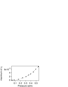
(a) Maximum of $J_{1}$. Dashed curve: quadratic fit

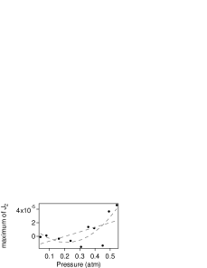
(b) Maximum of $J_{2}$. Dashed curves: linear and quadratic fits

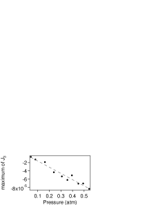
(c) Maximum of $J_{3}$. Dashed curve: linear fit

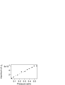
(d) Maximum of $J_{4}$. Dashed curve: linear fit

Figure 11: Evolution of the maximum of the $J(t)$ signals as a function of pressure.

Thus we can write:

$$J_{1} \simeq \overline{a}~{}S_{++},$$

$$J_{2} \simeq \Delta a_{2}~{}S_{++}+\Delta c_{2}~{}S_{--}+\Delta d_{2}~{}S_{-+},$$

$$J_{3} \simeq \overline{c}~{}S_{--},$$

$$J_{4} \simeq \overline{d}~{}S_{-+}.$$ (43)

The main contribution to $J_{4}$ comes from the Cotton-Mouton effect. We thus fit $J_{4}(t)$ with $\alpha B^{2}_{{}_{\perp},\mathrm{f}}(t)$. The value of $k_{\mathrm{CM}}$ is then calculated thanks to Eq. (42).

For the lowest pressures, the Cotton-Mouton signal, proportional to $\alpha B^{2}_{\perp,\mathrm{f}}$, also decreases. In this case, $\Delta a_{4}\,S_{++}$ and $\Delta c_{4}\,S_{--}$ are not completely negligible compared to $\alpha B^{2}_{\perp,\mathrm{f}}$. This is shown in Fig. 12 where a typical signal obtained for a helium pressure of $162\times 10^{-3}$ atm is plotted. We see that the fit of $J_{4}$ with $\alpha B^{2}_{\perp,\mathrm{f}}$ does not perfectly match the experimental data. To obtain a better fit, we have to add parameters. To this end, we first fix the value of $\alpha$ at the value obtained with the first fit $\alpha B^{2}_{\perp,\mathrm{f}}$. Then we fit $J_{4}$ with $\alpha B^{2}_{\perp,\mathrm{f}}+\alpha_{1}J_{1}+\alpha_{3}J_{3}$. $J_{2}$ is not used in this fit because, as said before, it is mainly a linear combination of the other signals. One can see in Fig. 12 that this fit now matches much better the data. We can conclude that, in this case, we have:

$$J_{4} = \alpha B^{2}_{\perp,\mathrm{f}}+\Delta a_{4}~{}S_{++}+\Delta c_{4}~{}S_{--},$$ (44)

$$= \alpha B^{2}_{\perp,\mathrm{f}}+\frac{\Delta a_{4}}{\overline{a}}~{}J_{1}+\frac{\Delta c_{4}}{\overline{c}}~{}J_{3},$$ (45)

with $\alpha_{2}=\Delta a_{4}/\overline{a}$ and $\alpha_{3}=\Delta c_{4}/\overline{c}$. This fit procedure repeated for each pressure shows that we always have $\alpha_{2}$ and $\alpha_{3}$ lower than 0.1.

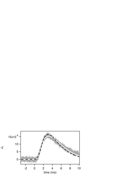
Figure 12: Gray: Time evolution of $J_{4}$ for a pressure of $162\times 10^{-3}$ atm. Black dashed curve: fit with $\alpha B^{2}_{\perp,\mathrm{f}}$. White solid curve: fit with $\alpha B^{2}_{\perp,\mathrm{f}}+\alpha_{1}J_{1}+\alpha_{3}J_{3}$, the value of $\alpha$ being fixed at the value obtained with the previous fit $\alpha B^{2}_{\perp,\mathrm{f}}$.

The value of $k_{\mathrm{CM}}$ as a function of the pressure is shown in Fig. 13. A linear fit of this data gives $k_{\mathrm{CM}}=(2.19\pm 0.09)\times 10^{-16}$ T^-2atm^-1 at $T=(293\pm 1)$K. Its $k_{\mathrm{CM}}$-axis intercept is consistent with zero within the uncertainties.

Figure 13: Linear magnetic birefringence of helium gas as a function of pressure. The solid line corresponds to the linear fit of the experimental data.

The A-type uncertainties come from the fit and from the photon lifetime with a relative variation lower than 2$\%$. The B-type uncertainties have been evaluated previously and detailed in Ref. Berceau2012 . They essentially come from the length of the magnetic field $L_{B}$. They are summarized in Table 4. We obtain for the value of the Cotton-Mouton constant at $T=(293\pm 1)$ K:

$$k_{\mathrm{CM}}=(2.19\pm 0.12)\times 10^{-16}\,\mathrm{T^{-2}atm^{-1}}.$$ (46)

The value of $k_{\mathrm{CM}}$ normalized at 273.15 K is calculated with a scale law on the gas density:

$$k_{\mathrm{CM}}=(2.35\pm 0.13)\times 10^{-16}\,\mathrm{T^{-2}atm^{-1}},$$ (47)

at $\lambda=1064$ nm, taking into account the uncertainty on the temperature.

Parameter	Typical value	Relative B-type
		uncertainty
$\alpha$	$10^{-5}$ rad T-2	$2.2\times 10^{-2}$
$\Delta^{\mathrm{FSR}}$	65.996 MHz	$3\times 10^{-4}$
$L_{B}$	0.137 m	$2.2\times 10^{-2}$
$\lambda$	1064.0 nm	$<5\times 10^{-4}$
$\sin 2\theta_{\mathrm{P}}$	1.0000	$9\times 10^{-4}$
Total		$3.1\times 10^{-2}$

Table 4: Parameters that have to be measured to infer the value of the Cotton-Mouton constant $k_{\mathrm{CM}}$ and their respective relative B-type uncertainty at 1$\sigma$.

IV.3.2 Comparison

The value of the Cotton-Mouton effect in helium is calculated very precisely thanks to ab initio quantum chemistry computational methods Rizzo2005 . Theoreticians concentrate on the calculation of the hypermagnetizability anisotropy $\Delta\eta$ while experimentalists measure the birefringence $\Delta n_{\mathrm{CM}}=k_{\mathrm{CM}}B^{2}$. The Cotton-Mouton constant $k_{\mathrm{CM}}$ is linked to $\Delta\eta$ by Rizzo1997 :

$$k_{\mathrm{CM}}\ [\mathrm{atm^{-1}T^{-2}}]=\frac{6.18381\times 10^{-14}}{T}\Delta\eta\ [\mathrm{a.u.}]$$ (48)

Few experiments were realized to measure the Cotton-Mouton effect of helium. The results are summarized in Table 5. The theoretical values correspond to the ones of Ref. Coriani1999 . The latter have been obtained using the Full Configuration Interaction (FCI) method and the most extended wave functions basis. They are expected therefore to be very accurate.

Experimental results			Theoretical prediction Coriani1999
Ref.	$\lambda$ [nm]	$10^{16}\times k_{\mathrm{CM}}~{}[T^{-2}]$	$10^{16}\times k_{\mathrm{CM}}~{}[T^{-2}]$
Cameron1991	$514.5$	$1.80\pm 0.36$	2.3959
Bregant2009	$532$	$2.08\pm 0.16$	2.3966
Muroo2003	$790$	$3.95\pm 1.40$	2.4018
Bregant2009	$1064$	$2.22\pm 0.16$	2.4036
This work	$1064$	$2.35\pm 0.13$	2.4036

Table 5: Experimental and theoretical values of Cotton-Mouton constant for helium gas. Values are normalized for a temperature of 273.15 K and a pressure of 1 atm. Uncertainties are given at 1$\sigma$.

Our result is compatible at better than 1$\sigma$ with the theoretical prediction and is the most precise value of $k_{\mathrm{CM}}$ ever measured, as we can see in Fig. 14 that summarizes the results for the Cotton-Mouton measurements at 273.15 K.

(a) Reported values for $\lambda$ ranging from 514.5 nm to 1064 nm

(b) Summary of the two values at $\lambda=1064$ nm

Figure 14: Comparison of reported values of Cotton-Mouton effect of helium gas. $\vartriangle$: experimental values of helium Cotton-Mouton constant reported in Refs. Cameron1991 ; Muroo2003 ; Bregant2009 . $\circ$: our experimental value. $\bullet$ and dashed line: theoretical predictions reported in Ref. Coriani1999 .

V Discussions and conclusion

In this paper we report a new measurement of Faraday and Cotton-Mouton effects at $\lambda=1064$ nm. Both measurements have precisions that are of the order of a few percent, corresponding to one of the most precise birefringence measurements. Our measurements are also accurate and they are in agreement with theory at better than 1$\sigma$.

As far as Faraday effect is concerned, our measurement is the first at $\lambda=1064$ nm. It is worthwhile to stress that our measurement is also absolute, while previous results Ingersoll1954 ; Ingersoll1956 were given with respect to the Faraday effect of water.

Our Cotton-Mouton measurement is the second experimental value at $\lambda=1064$ nm but it is the first to agree so well with the theoretical prediction. This definitely solves the problem of the discrepancy between experiment and theory originated from the first 1991 measurements and calculation Rizzo1997 and that still persisted (see Table 5).

The measurement of such small Cotton-Mouton effects, as the helium one, is not only important to test the quantum chemistry predictions. It is also a crucial test for the apparata devoted to the search of vacuum magnetic birefringence. Quantum electrodynamics predicts that a vacuum, as any other centro symmetric medium, should exhibit a Cotton-Mouton effect Battesti2013 . This fundamental prediction has not yet been experimentally proven. Several attempts have been made and a few are still under way Battesti2013 . Vacuum Cotton-Mouton effect should be about eight orders of magnitude smaller than the one of helium at 1 atm. Measurement of the Cotton-Mouton effect of helium is therefore compulsory in the search for improving the sensitivity of such apparata.

Our experimental method based on pulsed fields coupled to a Fabry-Pérot cavity seems very appropriate to reach the sensitivity needed for vacuum measurement. The measurements reported here validate the whole procedure of data taking and signal analysis that allow to isolate the main effect from the spurious ones thanks to signal symmetries. They are therefore a milestone in the road towards vacuum linear magnetic birefringence.