Eviction of a 125 GeV “heavy”-Higgs from the MSSM

Abstract

We prove that the present experimental constraints are already enough to rule out the possibility of the $\sim 125$ GeV Higgs found at LHC being the second lightest Higgs in a general MSSM context, even with explicit CP violation in the Higgs potential. Contrary to previous studies, we are able to eliminate this possibility analytically, using simple expressions for a relatively small number of observables. We show that the present LHC constraints on the diphoton signal strength, $\tau\tau$ production through Higgs and BR($B\to X_{s}\gamma$) are enough to preclude the possibility of $H_{2}$ being the observed Higgs with $m_{H}\simeq 125$ GeV within an MSSM context, without leaving room for finely tuned cancellations. As a by-product, we also comment on the difficulties of an MSSM interpretation of the excess in the $\gamma\gamma$ production cross section recently found at CMS that could correspond to a second Higgs resonance at $m_{H}\simeq 136$ GeV.

1 Introduction

In July 2012, both ATLAS and CMS, the two LHC general purpose experiments, announced the discovery of a bosonic resonance with a mass $\sim 125$ GeV that could be interpreted as the expected Higgs boson in the Standard Model (SM) Aad:2012tfa ; Chatrchyan:2012ufa . The observed production cross section and decay channels seem to be consistent, within errors, with a Higgs boson in the SM framework. However, at present, although CMS results are just below SM expectations, ATLAS shows a slight excess in the most sensitive channels that, if confirmed with more precise measurements, could be a sign of new physics beyond the single SM Higgs.

Besides, despite the extraordinary success of the SM in explaining all the experimental results obtained so far, both in the high energy as well as in the low energy region, there is a general belief that the SM is not the ultimate theory, but only a low energy limit of a more fundamental one. This underling, more fundamental theory is expected to contain new particles and interactions opening new processes not possible in the SM but, above all, it is envisaged to go one step further in the long way to reach a theory which incorporates gravity to our quantum field description of Nature. In such an endeavor, symmetries, who have historically played an important role in our understanding of the laws of Nature, are expected to be a major player. This is one of the reasons why Supersymmetry (SUSY), the only possible extension of symmetry beyond internal Lie symmetries and the Poincare group Coleman:1967ad ; Haag:1974qh , is arguably the most popular extension of the SM. SUSY is a symmetry between fermions and bosons, and, in its minimal version, the Minimal Supersymmetric Standard Model (MSSM), assigns a supersymmetric partner to each SM particle Fayet:1974pd ; Fayet:1977yc ; Farrar:1978xj ; Witten:1981nf ; Dimopoulos:1981zb ; Sakai:1981gr ; Ibanez:1981yh ; Kaul:1981wp ; Nilles:1983ge ; Haber:1984rc . These particles must have a mass close to the electroweak scale, if SUSY is to solve the hierarchy problem of the SM. Moreover, the MSSM requires a second Higgs doublet in addition to the single doublet present in the SM and, therefore, Higgs phenomenology in the MSSM is much richer than the SM, with three neutral-Higgs states and a charged Higgs in the spectrum Djouadi:2005gj .

At tree level, the scalar potential of the MSSM is CP-conserving, and therefore mass eigenstates are also CP eigenstates. We have two neutral scalar bosons, $h$ and $H$, and a neutral pseudoscalar, $A$. However, the MSSM contains several CP violating phases beyond the single SM phase in the CKM matrix, e.g. $M_{i},i=1,2,3$, $A_{t}$, $\mu$ are complex parameters, and then CP violation necessarily leaks into the Higgs sector at one-loop level Pilaftsis:1998dd ; Pilaftsis:1998pe ; Pilaftsis:1999qt ; Demir:1999hj . As a result, loop effects involving the complex parameters in the Lagrangian violate the tree-level CP-invariance of the MSSM Higgs potential modifying the tree-level masses, couplings, production rates and decay widths of Higgs bosons Pilaftsis:1999qt ; Carena:2000yi ; Choi:2000wz ; Carena:2001fw ; Choi:2001pg ; Choi:2002zp . In particular, the clear distinction between the two CP-even and the one CP-odd neutral boson is lost and the physical Higgs eigenstates become admixtures of CP-even and odd states. Therefore, significant deviations from the naive CP conserving scenario can be obtained in the regime where $M_{H^{\pm}}$ is low and Im $(\mu A_{t})$ is significant. Yet, the size of SUSY phases is strongly constrained by searches of electric dipole moments (EDM) of the electron and neutron. The phase of $\mu$ is bounded to be miserably small, $\lesssim 10^{-2}$, by the upper limits on EDMs if sfermion masses are below several TeV. Bounds on the phases of $A_{e,d,u}$, although somewhat weaker, are also strong, $\lesssim 10^{-1}$, under the same conditions. However, the phases of third generation trilinear couplings $A_{t,b,\tau}$ can still be sizeable for soft masses $O(1~{}\mbox{TeV})$ and, due to the large Yukawa couplings, these are precisely the couplings that influence the scalar potential more strongly Pilaftsis:1999td . In this work, we will take only third-generation trilinear couplings $A_{t,b,\tau}$ as complex to generate the scalar-pseudoscalar mixing in the Higgs potential.

Among all the possibilities opened up by this scenario, one particularly interesting is the case where the scalar observed at LHC is not the lightest but the second lightest one, having the lightest escaped detection at LEP/Tevatron/LHC due to its pseudoscalar or down-type content. As a result of the mixing, the couplings $H_{1}-WW$, $H_{1}-ZZ$ and $H_{1}-t\bar{t}$ all get reduced simultaneously evading the current bounds. This idea of course is not new. Many studies have been carried out within this model Heinemeyer:2011aa ; Hagiwara:2012mga ; Arbey:2012dq ; Bechtle:2012jw ; Ke:2012zq ; Ke:2012yc ; Moretti:2013lya ; Scopel:2013bba . There are two public codes, CPsuperH Lee:2003nta ; Lee:2012wa , specifically developed to analyze the Higgs phenomenology in the MSSM with explicit CP violation, and FeynHiggs Heinemeyer:1998yj ; Hahn:2005cu , that also calculates the spectrum and decay widths of the Higgses in the Complex MSSM. By using them, different regions of the parameters space have been explored through giant scans following the results of the colliders.

In this work, we will explore a different path. We will study this scenario, not by scanning its parameters space but rather by choosing a pair of key experimental signatures from both, high and low energy experiments, and analyzing (analytically or semi-analytically) whether their results can be simultaneously satisfied. This way we gain understanding on the physics of the model we are discussing and at the same time avoid the possibility of missing a fine-tuned region in the parameter space (even tiny to the point of being microscopic) where an unexpected cancellation or a lucky combination might occur. After all, whatever physics hides so effectively behind the SM will turn out to be just one point in our studies of the parameter space. In this sense it is clear that every region, independently of its size, has the same probability of being the right one and should be given enough attention.

Moreover, our analysis is performed in terms of the SUSY parameters at the electroweak scale, such that it encloses all possible MSSM setups (including explicit CP violation), as the CMSSM, NUHM, pMSSM or even a completely generic MSSMEllis:2002wv ; Ellis:2002iu ; Ellis:2008eu ; Berger:2008cq ; AbdusSalam:2009qd ; Arbey:2012dq ; Arbey:2012bp . In fact, only a handful of MSSM parameters affect the Higgs sector and low-energy experiments that we study. As we will see, in the Higgs sector, we fix $m_{H_{1}}\leq m_{H_{2}}\simeq 125~{}\mbox{GeV}\leq m_{H_{3}}\simeq m_{H^{\pm}}\lesssim 200$–220 GeV and use the experimental results to look for acceptable, $3\times 3$, Higgs mixing matrices as a function of $\tan\beta$. Supersymmetric parameters affecting the Higgs sector, and also the indirect processes $B\to X_{s}\gamma$ and $B_{s}\to\mu^{+}\mu^{-}$, are basically third generation masses and couplings, and gaugino masses. In our analysis, these parameters take general values consistent with the experimental constraints on direct and indirect searches.

This paper is organized as follows. We begin by summarizing the experimental situation in Section 2. In Section 3 we describe the basic ingredients of the model and analyze the direct and indirect signatures we will choose for our study. The parameter space is surveyed in Section 4 and results and conclusions are contained in Section 5.

2 Current experimental status.

2.1 Higgs signal at the LHC.

Both ATLAS and CMS experiments have recently updated the analysis of the Higgs-like signal using the full $pp$ collision data sample. The ATLAS analysis ATLAS-CONF-2013-034 uses integrated luminosities of 4.8 fb^-1 at $\sqrt{s}=$7 TeV plus 20.7 fb^-1 at $\sqrt{s}=$8 TeV, for the most sensitive channels, $H\rightarrow\gamma\gamma$, $H\rightarrow ZZ^{*}\rightarrow 4l$ and $H\rightarrow WW^{*}\rightarrow l\nu l\nu$, plus 4.7 fb^-1 at $\sqrt{s}=$7 TeV and 13 fb^-1 at $\sqrt{s}=$8 TeV for the $H\rightarrow\tau\tau$ and $H\rightarrow b\bar{b}$. Similarly CMS study CMS-PAS-HIG-13-005 uses 5.1 fb^-1 at $\sqrt{s}=$7 TeV and 19.8 fb^-1 at $\sqrt{s}=$8 TeV in all these channels.

The main channels contributing to the observed signal are the decays into photons and two Z-bosons. On the other hand, the most relevant channel constraining the presence of additional Higgs-bosons is the decay into two $\tau$ leptons. ATLAS and CMS agree on the mass of the observed state which is $m_{h}=124.3\pm 0.6(\mbox{stat)$\pm$0.4(\mbox{sist)}}$ GeV for ATLAS and $m_{h}=125.7\pm 0.3(\mbox{stat})\pm 0.3(\mbox{sist})$ GeV for CMS.

However, there are some differences on the signal strength in the different channels as measured by the two experiments. The signal strength $\mu_{X}$, for a Higgs decaying to $X$ is defined as,

$$\mu_{X}=\frac{\sigma(pp\to H)\times\mbox{BR}(H\to X)}{\sigma(pp\to H)_{\rm{SM}}\times\mbox{BR}(H\to X)_{\rm{SM}}},$$ (1)

such that $\mu=0$ corresponds to the background-only hypothesis and $\mu=1$ corresponds to a SM Higgs signal. The combined signal strength in the last results presented by ATLAS is $\mu^{\rm{ATLAS}}=1.3\pm 0.2$ Aad:2013wqa , while the signal strength measured by CMS is slightly below the SM expectations $\mu^{\rm{CMS}}=0.80\pm 0.14$ CMS-PAS-HIG-13-005 .

For the diphoton channel, the measured signal strength in both experiments are $\mu_{\gamma\gamma}^{\rm{ATLAS}}=1.6\pm 0.3$ and $\mu_{\gamma\gamma}^{\rm{CMS}}=0.78_{-0.26}^{+0.28}$. This signal is consistent with the SM, although ATLAS points to a slight excess over the SM expectations. In any case, both results agree on the fact that the diphoton signal must be of the order of the SM prediction. This fact is very important in the context of multi-Higgs models, as the MSSM, where the Higgs couplings to down quark and charged leptons are enhanced by additional $\tan\beta$ factors, which tend to decrease the $H\to\gamma\gamma$ branching ratio and therefore the signal strength. In this regard, here we will adopt a conservative approach and impose the weighted average of ATLAS and CMS results at 2$\sigma$,

$$0.75\leq\mu_{\gamma\gamma}^{\rm{LHC}}\leq 1.55\,.$$ (2)

Similarly, the signal strength in the $H\to ZZ^{*}$ channel are, $\mu_{ZZ^{*}}^{\rm{ATLAS}}=1.5\pm 0.4$ and $\mu_{ZZ^{*}}^{\rm{CMS}}=0.92\pm 0.28$ and we will also use as a constraint,

$$0.78\leq\mu_{ZZ^{*}}^{\rm{LHC}}\leq 1.58\,.$$ (3)

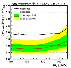
(a)

(b)

Figure 1: Higgs searches in the $H\rightarrow\tau\tau$ channel for $100~{}\mbox{GeV}\leq m_{H}\leq 150~{}\mbox{GeV}$ at CMS (a) and ATLAS (b).

The main constraint on the presence of additional heavy Higgs states comes from the $H/A\rightarrow\tau\tau$ searches at ATLAS and CMS experiments. In this case, both experiments have searched for the SM Higgs boson decaying into a pair of $\tau$-leptons and this provides a limit on $\sigma(pp\to H)\times\mbox{BR}(H\to\tau\tau)$ that can be applied to the extra Higgs states. ATLAS has analyzed the collected data samples of $4.6\,\mbox{fb}^{-1}$at $\sqrt{s}=$7 TeV and $13.0\,\mbox{fb}^{-1}$at $\sqrt{s}=$8 TeV Aad:2012mea while CMS used $4.9\,\mbox{fb}^{-1}$at $\sqrt{s}=$7 TeV and $19.4\,\mbox{fb}^{-1}$at $\sqrt{s}=$8 TeV for Higgs masses up to 150 GeV CMS-PAS-HIG-13-004 . These constraints on the $\tau\tau$-cross section normalized to the SM cross section as a function of the Higgs mass are shown in Figure 1. In this case, CMS sets the strongest bound for $m_{H}$ below 150 GeV. For $m_{H}=110$ GeV we obtain a bound at 95% CL of $\mu_{\tau\tau}=\sigma\left(H\rightarrow\tau\tau\right)/\sigma_{SM}\leq 1.8$, and this limit remains nearly constant, $\mu_{\tau\tau}\leq 2.0$, up to $m_{H}=140$ GeV. For a neutral Higgs of mass $m_{H}=150$ GeV we would have a bound of $\mu_{\tau\tau}\leq 2.3$. In our scenario, this limit would apply to $H_{1}$ with a mass below 125 GeV and to $H_{2}$ with $m_{H_{2}}\simeq 125$ GeV. In the case of $H_{3}$, this bound applies for masses below 150 GeV.

For heavier $H_{3}$ masses, there exist a previous analysis at LHC searching MSSM Higgs bosons with masses up to 500 GeV. In Figure 2, we present the analysis made in ATLAS with $4.9\,\mbox{fb}^{-1}$ at $\sqrt{s}=$7 TeV Aad:2012yfa . In this case, the bound is presented as an upper limit on the $\tau\tau$, or $\mu\mu$ production cross section. As a reference, the SM cross section for a Higgs mass of 150 GeV is $\sigma(pp\to H)_{\rm{SM}}\times\mbox{BR}(H\to X)_{\rm{SM}}\simeq 0.25$ pb and therefore, comparing with Figure 1, we can expect this bound to improve nearly an order of magnitude in an updated analysis with the new data privateFiorini . Nevertheless, the production cross-section of $\tau$-pairs through a heavy Higgs is enhanced by powers of $\tan\beta$ and therefore the present limits on $\sigma_{\phi}\times\mbox{BR}(\phi\to\tau\tau)$ are already very important in the medium–large $\tan\beta$ region.

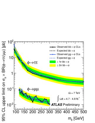
Figure 2: Upper limit on the $\tau\tau$ production cross section through heavy Higgs states from ATLAS with $4.8~{}\mbox{fb}^{-1}$ at $\sqrt{s}=7$ TeV .

Finally, we include the bounds on charged Higgs produced in $t\to H^{+}b$ with subsequent decay $H^{+}\to\tau\nu$ Aad:2012tj ; CMS-PAS-HIG-12-052 . These analysis set upper bounds on $B(t\to H^{+}b)$ in the range 2–3 % for charged Higgs bosons with masses between 80 and 160 GeV, under the assumption that $B(H^{+}\to\tau^{+}\nu_{\tau})=1$, which is a very good assumption unless decay channels to the lighter Higgses and W-bosons are kinematically opened.

2.2 MSSM searches at LHC.

Simultaneously to the Higgs searches described above, LHC has been looking for signatures on new physics beyond the SM. A large effort has been devoted to search for Supersymmetric extensions of the SM. These studies, focused in searches of jets or leptons plus missing energy (possible evidence of the LSP), agree, so far, with the Standard Model expectations in all the explored region, and are used to set bounds on the mass of the supersymmetric particles.

The most stringent constraints from LHC experiments are set on gluinos and first generation squarks produced through strong interactions in $pp$ collisions. Searches of gluinos at CMSChatrchyan:2012paa ; Chatrchyan:2013wxa ; PAS-SUS-13-007 ; PAS-SUS-13-008 and ATLAS ATLAS-CONF-2012-145 ; ATLAS-CONF-2013-007 with $\sim 20$ fb^-1 at 8 TeV have driven, roughly, to the exclusion of gluino masses up to 1.3 TeV for (neutralino) LSP masses below 500 GeV. The limits on first generation squarks directly produced are $m_{\tilde{q}}\gtrsim 740$ GeV for squarks decaying $\tilde{q}\to q\chi_{1}^{0}$ with $m_{\chi_{1}^{0}}=0$ GeVChatrchyan:2013lya .

The most important players in Higgs physics, because of their large Yukawa couplings, are third generation squarks. In this case mass bounds, from direct stop production, are somewhat weaker but still stop masses are required to be above $\sim 650$ GeV for $m_{\chi^{0}}\lesssim 200$ GeV ATLAS-CONF-2013-024 ; ATLAS-CONF-2013-037 ; ATLAS-CONF-2013-053 ; PAS-SUS-13-011 with the exception of small regions of nearly degenerate stop-neutralino. Limits on sbottom mass from direct production are also similar and sbottom masses up to 620 GeV are excluded at 95% C.L. for $m_{\chi^{0}}<150$ GeV, with the exception of $m_{{\tilde{b}}_{1}}-m_{\chi^{0}}<70$ GeV ATLAS-CONF-2013-053 ; Chatrchyan:2013lya ; PAS-SUS-13-008 .

Finally, ATLAS and CMS have presented the limits on chargino masses from direct EW production ATLAS-CONF-2013-035 ; PAS-SUS-12-022 . In both analysis, these limits depend strongly on the slepton masses and the branching ratios of chargino and second neutralino that are supposed to be degenerate. When the decays to charged sleptons are dominant, chargino masses are excluded up to $\sim 600$ GeV for large mass differences with $\chi^{0}$. Even in the case when the slepton channels are closed, decays to weak bosons plus lightest neutralino can exclude chargino masses up to $\sim 350$ GeV for $m_{\chi_{1}^{0}}\lesssim 120$ GeV.

Therefore, as we have seen, limits on SUSY particles from LHC experiments are already very strong with the exceptions of sparticle masses rather degenerate with the lightest supersymmetric particle.

2.3 Indirect bounds

Indirect probes of new physics in low energy experiments still play a very relevant role in the search for extensions of the SM Masiero:2001ep ; Raidal:2008jk ; Calibbi:2011dn . Even in the absence of new flavour structures beyond the SM Yukawa couplings, in a Minimal Flavour Violation scheme, decays like $B_{s}^{0}\rightarrow\mu^{+}\mu^{-}$ and, specially, $B\rightarrow X_{s}\gamma$ play a very important role, as we will see below, and put significant constraints for the whole $\tan\beta$ range.

The present experimental bounds on the decay $B_{s}^{0}\rightarrow\mu^{+}\mu^{-}$ are obtained from LHCb measurements with 1.1 fb^-1 of proton-proton collisions at $\sqrt{s}=8$ TeV and 1.0 fb^-1 at $\sqrt{s}=7$ TeV. The observed value for the branching ratio at LHCb Aaij:2012nna ; Aaij:2013aka is,

$$\mbox{BR}\left(B_{s}^{0}\rightarrow\mu^{+}\mu^{-}\right)=\left(2.9^{+1.1}_{-1.0}\right)\times 10^{-9}\,,$$ (4)

and at CMS Chatrchyan:2013bka ,

$$\mbox{BR}\left(B_{s}^{0}\rightarrow\mu^{+}\mu^{-}\right)=\left(3.0^{+1.0}_{-0.9}\right)\times 10^{-9}\,,$$ (5)

The limits on the decay $B\rightarrow X_{s}\gamma$ come from the BaBar and Belle B-factories and CLEO Chen:2001fja ; Abe:2001hk ; Limosani:2009qg ; Lees:2012wg ; Lees:2012ufa ; Aubert:2007my . The current world average for $E_{\gamma}>1.6$ GeV given by HFAG Amhis:2012bh ; hfag is,

$$\mbox{BR}\left(B\rightarrow X_{s}\gamma\right)=\left(3.43\pm 0.21\pm 0.07\right)\times 10^{-4}\,.$$ (6)

We will see that this result provides a very important constraint on the charged Higgs mass in the low $\tan\beta$ region where other supersymmetric contributions are small.

3 Theoretical model

As explained in the introduction, we intend to investigate whether the observed Higgs particle of $m_{H}\simeq 125$ GeV could correspond to the second Higgs in a general MSSM scenario, while the lightest Higgs managed to evade the LEP searches Heinemeyer:2011aa ; Hagiwara:2012mga ; Arbey:2012dq ; Bechtle:2012jw ; Ke:2012zq ; Ke:2012yc ; Moretti:2013lya ; Scopel:2013bba . The scenario we consider here is a generic MSSM defined at the electroweak scale. This means we do not impose the usual mass relations obtained through RGE from a high scale, that we obtain, for instance in the Constrained MSSM (CMSSM), but keep all MSSM parameters as free and independent at $M_{W}$. Furthermore, we are mainly interested in the Higgs sector of the model, which we analyze assuming generic Higgs masses and mixings in the presence of CP violation in the squark sector.

3.1 CP-violating MSSM Higgs sector

As it is well-known, the Higgs sector of the MSSM consists of a type II two-Higgs doublet model. In the MSSM, the scalar potential conserves CP at tree-level Djouadi:2005gj . Nevertheless, in the presence of complex phases in the Lagrangian, CP violation enters the Higgs potential at the one-loop level, resulting in the mixing between the CP-even and CP-odd Higgses. Then, after electroweak symmetry breaking, we have three physical neutral scalar bosons, admixtures of the scalar and pseudoscalar Higgs bosons, plus a charged Higgs boson Pilaftsis:1998dd ; Pilaftsis:1998pe ; Pilaftsis:1999qt ; Demir:1999hj .

The Higgs fields in the electroweak vacuum, with vevs $\upsilon_{1}$and $\upsilon_{2}$ and $\tan\beta=\upsilon_{2}/\upsilon_{1}$, are

$$\Phi_{1}=\left(\begin{array}[]{c}\frac{1}{\sqrt{2}}\left(\upsilon_{1}+\phi_{1}+ia_{1}\right)\\ \phi_{1}^{-}\end{array}\right);\;\;\Phi_{2}=e^{i\xi}\left(\begin{array}[]{c}\phi_{2}^{+}\\ \frac{1}{\sqrt{2}}\left(\upsilon_{2}+\phi_{2}+ia_{2}\right)\end{array}\right)\,,$$ (7)

and, as mentioned above, the presence of CP-violating phases in the Lagrangian introduces off-diagonal mixing terms in the neutral Higgs mass matrix. In the weak basis, $\left(\phi_{1},\phi_{2},a\right)$, with $\phi_{1,2}$ CP-even, scalar, and $a=a_{1}\sin\beta+a_{2}\cos\beta$ the CP-odd, pseudoscalar state, we write the neutral Higgs mass matrix as Pilaftsis:1999qt ; Carena:2000yi ; Carena:2001fw ; Funakubo:2002yb ,

$$M_{H}^{2}=\left(\begin{array}[]{cc}M_{S}^{2}&M_{SP}^{2}\\ M_{PS}^{2}&M_{P}^{2}\end{array}\right)\,,$$ (8)

where the scalar-pseudoscalar mixings are non-vanishing in the presence of phases, $M_{SP}^{2},M_{PS}^{2}\propto\mbox{Im}\left[\mu A_{t,b}e^{i\xi}\right]$. Then, this $3\times 3$ neutral Higgs mass matrix is diagonalized by

$${\cal U}\cdot M_{H}^{2}\cdot{\cal U}^{T}=\mbox{Diag}\left(m_{H_{1}}^{2},m_{H_{2}}^{2},m_{H_{3}}^{2}\right)\,.$$ (9)

The Higgs sector of the MSSM is defined at the electroweak scale at tree-level by only two parameters that, in the limit of CP-conservation, are taken as $\left(m_{A}^{2},\tan\beta\right)$. In the complex MSSM, the pseudoscalar Higgs is not a mass eigenstate and its role as a parameter defining the Higgs sector is played by the charged Higgs mass $m_{H^{\pm}}^{2}$. At higher orders, the different MSSM particles enter in the Higgs masses and mixings, although the main contributions are due to the top-stop and bottom–sbottom sectors. It is well-known that the one-loop corrections to $M_{S}^{2}$ can increase the lightest Higgs mass from $\lesssim M_{Z}$ to $\sim 130$ GeV Okada:1990vk ; Ellis:1990nz ; Haber:1990aw , hence being $\lesssim M_{Z}$, with the leading part of order Haber:1996fp ; Djouadi:2013vqa ,

$$\delta M_{S}^{2}\simeq\frac{3m_{t}^{4}}{2\pi^{2}\upsilon^{2}\sin^{2}\beta}\left[\log\frac{M_{SUSY}^{2}}{m_{t}^{2}}+\frac{X_{t}^{2}}{M_{SUSY}^{2}}\left(1-\frac{X_{t}^{2}}{12M_{SUSY}^{2}}\right)\right]\,,$$ (10)

with $M_{SUSY}$ the geometric mean of the two stop masses and $X_{t}=A_{t}-\mu\cot\beta$.

Regarding the charged Higgs mass, we can relate it to the pseudoscalar mass $M_{P}^{2}$ in the neutral Higgs mass matrix Pilaftsis:1999qt ,

$$M_{H^{\pm}}^{2}=M_{P}^{2}+\frac{1}{2}\lambda_{4}\upsilon^{2}-\mbox{Re}\left(\lambda_{5}e^{2i\xi}\right)\upsilon^{2}\,,$$ (11)

with $\lambda_{4,5}$ the two-loop corrected parameters of the Higgs potential Carena:1995bx ; Pilaftsis:1999qt . At tree level $\lambda_{4}=g_{w}^{2}/2$, such that $\lambda_{4}\upsilon^{2}/2=M_{W}^{2}$, and $\lambda_{5}=$0. In any case, it looks reasonable to expected $\lambda_{i}\lesssim 1$. This implies that the squared charged Higgs mass can never be heavier that the largest neutral Higgs eigenvalue by a difference much larger than $M_{Z}^{2}$, which is equivalent to say that loop corrections are of the same order as $\sim\delta M_{S}^{2}$.

Similarly, we can expect the mass of the second neutral Higgs, which in our scenario is $m_{H_{2}}\simeq 125$ GeV, only to differ from the heavier eigenvalue by terms of order $\upsilon^{2}$. This can be seen from the trace of the neutral Higgs masses in the basis of CP eigenstates, where we would have, without loop corrections, $\mbox{Tr}\left(M_{H}^{2}\right)=2M_{P}^{2}+M_{Z}^{2}$. As we have seen, loop corrections to the diagonal elements can be expected to be of the order of the corrections to the lightest Higgs mass which are also $O(M_{Z}^{2})$. To obtain a light second Higgs we need, either low $M_{P}$ or a large scalar-pseudoscalar mixing. The different contributions to scalar-pseudoscalar mixing, $M_{SP}^{2}$, are of order Pilaftsis:1999qt ,

$$M_{SP}^{2}=O\left(\frac{m_{t}^{4}|\mu||A_{t}|}{32\pi^{2}~{}\upsilon^{2}M_{SUSY}^{2}}\right)\sin\phi_{CP}\times\left[6,\frac{|A_{t}|^{2}}{M_{SUSY}^{2}},\frac{|\mu|^{2}}{\tan\beta M_{SUSY}^{2}}\right]\,,$$ (12)

which again are of the same order as $\delta M_{S}^{2}\simeq O(M_{Z}^{2})$ for $\sin\phi_{CP}\sim O(1)$. Therefore, taking also into account that in the decoupling limit, and in the absence of scalar-pseudoscalar mixing, $M_{H}\simeq M_{P}$, we must require $M_{P}^{2}$ not to be much larger than $M_{Z}^{2}$. Taking $M_{P}^{2}\lesssim 3M_{Z}^{2}$, the invariance of the trace tells us that $m_{H_{1}}^{2}+m_{H_{2}}^{2}+m_{H_{3}}^{2}=2M_{P}^{2}+M_{Z}^{2}+O(M_{Z}^{2})$ in such a way that with $90~{}\mbox{GeV}\lesssim m_{H_{1}}\lesssim m_{H_{2}}\simeq 125$ GeV, we get an upper limit for $m_{H_{3}}^{3}\lesssim 2M_{P}^{2}+2M_{Z}^{2}-\left(m_{H_{2}}^{2}+m_{H_{1}}^{2}\right)\lesssim(200~{}\mbox{GeV})^{2}$. We must emphasize that in this work we do not consider the possibility of $m_{H_{1}}\lesssim 90~{}\mbox{GeV}$ which would be possible in the presence of large CP-violating phases that could reduce the mass of the lightest Higgs through rather precise cancellations Carena:2000ks ; Carena:2002bb . Although this scenario could survive LEP limits around an “open hole” with $m_{H_{1}}\approx 45~{}\mbox{GeV}$ and $\tan\beta\approx 8$ Williams:2007dc , it would never be able to reproduce the observed signal in $H_{2}\to\gamma\gamma$, as the opening of the decay channel $H_{2}\to H_{1}H_{1}$ would render $B(H_{2}\to\gamma\gamma)$ much smaller than the SM one (see the discussion related to the $H_{2}\to b\bar{b}$ channel below).

In the following analysis of the direct and indirect constraints on the Higgs sector, we try to be completely general in the framework of a Complex MSSM defined at the electroweak scale. To attain this objective, and taking into account that the presence of CP violation and large radiative corrections strongly modifies the neutral Higgs mass matrix if we are outside the decoupling regime, we consider general neutral Higgs mixings and masses. In fact, in this work, we analyze the situation in which the second lightest neutral boson corresponds to the scalar resonance measured at LHC with a mass of 125 GeV. As we have seen, to achieve this, we need a relatively light charged Higgs (with approximately $M_{H^{+}}\lesssim 220\,$ GeV), and a similar mass for the heaviest neutral Higgs. The lightest neutral Higgs boson will have a mass varying in the range of 90 and 125 GeV. After fixing the Higgs masses in these ranges, we will consider generic mixing matrices ${\cal U}$ and look for mixings consistent with the present experimental results.

This analysis deals with the decays of the neutral Higgs bosons. Thus we need the Higgs couplings to the SM vector boson, fermions, scalars and gauginos. The conventions used in the following are described in Appendix A. The couplings to the vector bosons are Lee:2003nta ,

$${\cal L}_{H_{a}V}=g\,M_{W}\left(W_{\mu}^{+}W^{-\,\mu}+\frac{1}{2\cos^{2}\theta_{W}}Z_{\mu}Z^{\mu}\right)\sum_{a}g_{H_{a}VV}\,H_{a}\,.$$ (13)

with $g_{H_{a}VV}=\cos\beta\,\mathcal{U}_{a1}+\sin\beta\,\mathcal{U}_{a2}$.

The Lagrangian showing the fermion–Higgs couplings is

$${\cal L}_{H_{a}f}=-\sum_{f}\frac{g\,m_{f}}{2M_{W}}\sum_{a}H_{a}\bar{f}\left(g_{S,a}^{f}+ig_{P,a}^{f}\gamma_{5}\right)f\,,$$ (14)

$\mathbf{H_{a}\rightarrow f\bar{f}}$	$\mathbf{g_{f}}$	$\mathbf{g_{S,a}^{(0)}}$	$\mathbf{g_{P,a}^{(0)}}$
$H_{a}\rightarrow l\bar{l}$	$\frac{gm_{l}}{2M_{W}}$	$\frac{U_{a1}}{\cos(\beta)}$	$-\left(\frac{\sin(\beta)}{\cos(\beta)}\right)U_{a3}$
$H_{a}\rightarrow d\bar{d}$	$\frac{gm_{d}}{2M_{W}}$	$\frac{U_{a1}}{\cos(\beta)}$	$-\left(\frac{\sin(\beta)}{\cos(\beta)}\right)U_{a3}$
$H_{a}\rightarrow u\bar{u}$	$\frac{gm_{u}}{2M_{W}}$	$\frac{U_{a2}}{\sin(\beta)}$	$-\left(\frac{\cos(\beta)}{\sin(\beta)}\right)U_{a3}$
$H_{a}\rightarrow\tilde{\chi}_{i}^{+}\tilde{\chi}_{j}^{-}$	$\frac{g}{\sqrt{2}}$	$g_{s}^{\tilde{\chi}^{+}}$	$g_{p}^{\tilde{\chi}^{+}}$

Table 1: Tree level Higgs–fermion couplings.

where the tree-level values of $(g_{S}^{(0)},g_{P}^{(0)})$ are given in Table 1. Still, in the case of third generation fermions, these couplings receive very important threshold corrections due to gluino and chargino loops enhanced by $\tan\beta$ factors in the case of the down-type fermions Hall:1993gn ; Carena:1994bv ; Blazek:1995nv ; Carena:1999py ; Hamzaoui:1998nu ; Babu:1999hn ; Isidori:2001fv ; Dedes:2002er ; Buras:2002vd . The complete corrected couplings for third generation fermions, $(g_{S}^{f},g_{P}^{f})$, can be found in Ref. Lee:2003nta ; Carena:2002bb . In our analysis, it is sufficient to consider the correction to the bottom couplings,

$$g_{S,a}^{d}=\mbox{Re}\left(\frac{1}{1+\kappa_{d}\tan\beta}\right)\frac{{\cal U}_{a1}}{\cos\beta}+\mbox{Re}\left(\frac{\kappa_{d}}{1+\kappa_{d}\tan\beta}\right)\frac{{\cal U}_{a2}}{\cos\beta}+\mbox{Im}\left(\frac{\kappa_{d}\left(\tan^{2}\beta+1\right)}{1+\kappa_{d}\tan\beta}\right){\cal U}_{a3}$$ (15)

$$g_{P,a}^{d}=-\mbox{Re}\left(\frac{\tan\beta-\kappa_{d}}{1+\kappa_{d}\tan\beta}\right){\cal U}_{a3}+\mbox{Im}\left(\frac{\kappa_{d}\tan\beta}{1+\kappa_{d}\tan\beta}\right)\frac{{\cal U}_{a1}}{\cos\beta}-\mbox{Im}\left(\frac{\kappa_{d}}{1+\kappa_{d}\tan\beta}\right)\frac{{\cal U}_{a2}}{\cos\beta}$$ (16)

where $\kappa_{d}=(\Delta h_{d}/h_{d})/(1+\delta h_{d}/h_{d})$ and the corrected Yukawa couplings are,

$$h_{d}=\frac{\sqrt{2}m_{d}}{\upsilon\cos\beta}\>\frac{1}{1+\delta h_{d}/h_{d}+\Delta h_{d}/h_{d}\tan\beta}\,,$$ (17)

$$\delta h_{d}/h_{d} = -\frac{2\alpha_{s}}{3\pi}m_{\tilde{g}}^{*}A_{d}\,I(m_{\tilde{d}_{1}}^{2},m_{\tilde{d}_{2}}^{2},|m_{\tilde{g}}|^{2})-\frac{|h_{u}|^{2}}{16\pi^{2}}|\mu|^{2}\,I(m_{\tilde{u}_{1}}^{2},m_{\tilde{u}_{2}}^{2},|\mu|^{2})$$

$$\Delta h_{d}/h_{d} = \frac{2\alpha_{s}}{3\pi}m_{\tilde{g}}^{*}\mu^{*}\,I(m_{\tilde{d}_{1}}^{2},m_{\tilde{d}_{2}}^{2},|m_{\tilde{g}}|^{2})+\frac{|h_{u}|^{2}}{16\pi^{2}}A_{u}^{*}\mu^{*}\,I(m_{\tilde{u}_{1}}^{2},m_{\tilde{u}_{2}}^{2},|\mu|^{2})\>,$$ (18)

and the loop function $I(a,b,c)$ is given by,

$$I(a,b,c)=\frac{a\,b\log(a/b)+b\,c\log(b/c)+a\,c\log(c/a)}{(a-b)(b-c)(a-c)}\,.$$ (19)

The Higgs-sfermion couplings are,

$${\cal L}_{H_{a}\tilde{f}\tilde{f}}=\upsilon\sum_{\tilde{f}}g_{\tilde{f}\tilde{f}}^{a}\left(H_{a}\tilde{f}^{*}\tilde{f}\right)\,,$$ (20)

$$\upsilon~{}g_{\tilde{f}_{i}\tilde{f}_{j}}^{a}=\left(\tilde{\Gamma}^{\alpha ff}\right)_{\beta\gamma}{\cal U}_{a\alpha}~{}{\cal R}^{f}_{\beta i}{\cal R}^{f}_{\gamma j}\,,$$ (21)

with $\beta,\gamma=L,R$, ${\cal R}^{f}$, the sfermion mixing matrices and the couplings $\tilde{\Gamma}^{\alpha ff}$ given Ref. Lee:2003nta . Other Higgs couplings that are needed to analyze the neutral Higgs decays are the couplings to charginos and charged Higgs, complete expressions can be found in Ref. Lee:2003nta (taking into account their different convention on the Higgs mixing matrix, ${\cal U}={\cal O}^{T}$).

After defining all these couplings, we show in the following the expressions for $H\to\gamma\gamma$ and $H\to gg$, that together with $H\rightarrow\bar{b}b,\tau\tau$ and $H\to WW^{*},ZZ^{*}$ are the main Higgs decay channels for $m_{H}=125$ GeV, and the Higgs production mechanisms at LHC.

3.2 Higgs decays.

3.2.1 Higgs decay into two photons.

The decay $H_{a}\to\gamma\gamma$ occurs only at the one-loop level and therefore we must include every contribution generated by sparticles in addition to the SM ones in our calculation. Taking into account the presence of CP violation, the Higgs decay has contributions of both the scalar and pseudoscalar components. Then its width becomes,

$$\Gamma\left(H_{a}\rightarrow\gamma\gamma\right)=\frac{M_{H_{a}}^{3}\alpha^{2}}{256\pi^{3}\upsilon^{2}}\left[\left|S_{a}^{\gamma}\left(M_{H_{a}}\right)\right|^{2}+\left|P_{a}^{\gamma}\left(M_{H_{a}}\right)\right|^{2}\right]\,,$$ (22)

where the scalar part is $S_{a}^{\gamma}\left(M_{H_{a}}\right)$ and the pseudoscalar $P_{a}^{\gamma}\left(M_{H_{a}}\right)$ and they are Lee:2003nta ,

$$S_{a}^{\gamma}\left(M_{H_{a}}\right) = 2\underset{f=b,t,\tilde{\chi}_{1}^{\pm},\tilde{\chi}_{2}^{\pm}}{\sum}N_{C}\,J_{f}^{\gamma}\,Q_{f}^{2}g_{f}\,g_{H_{a}\bar{f}f}^{S}\frac{\upsilon}{m_{f}}F_{f}^{S}\left(\tau_{af}\right)-\sum_{\tilde{f}}N_{C}\,J_{\tilde{f}}^{\gamma}\,Q_{f}^{2}\,g_{H_{a}\tilde{f}_{j}\tilde{f_{j}^{*}}}^{S}\frac{\upsilon^{2}}{2m_{\tilde{f}_{j}}^{2}}F_{0}\left(\tau_{a\tilde{f}_{j}}\right)$$ (23)

$$-g_{H_{a}VV}F_{1}\left(\tau_{aW}\right)~{}-~{}g_{H_{a}H^{-}H^{+}}\frac{\upsilon^{2}}{2M_{H_{a}}^{2}}F_{0}\left(\tau_{aH}\right)$$

$$P_{a}^{\gamma}\left(M_{H_{a}}\right) = 2\underset{f=b,t,\tilde{\chi}_{1}^{\pm},\tilde{\chi}_{2}^{\pm}}{\sum}N_{C}\,J_{f}^{\gamma}\,Q_{f}^{2}g_{f}\,g_{H_{a}\bar{f}f}^{P}\frac{\upsilon}{m_{f}}F_{f}^{P}\left(\tau_{af}\right)$$ (24)

With $\tau_{aj}=M_{H_{a}}^{2}/(4m_{i}^{2})$ and the loop functions being:

$$\begin{array}[]{ll}F_{f}^{S}\left(\tau\right)=\tau^{-1}\left[1+\left(1-\tau^{-1}\right)f\left(\tau\right)\right];&F_{f}^{P}\left(\tau\right)=\tau^{-1}f\left(\tau\right);\\ F_{0}\left(\tau\right)=\tau^{-1}\left[-1+\tau^{-1}f\left(\tau\right)\right];&F_{1}\left(\tau\right)=2+3\tau^{-1}+3\tau^{-1}\left(2-\tau^{-1}\right)f\left(\tau\right);\end{array}$$ (25)

$$f\left(\tau\right)=-\frac{1}{2}\intop\nolimits_{0}^{1}\frac{\mathrm{d}x}{x}\ln\left[1-4\tau x\left(1-x\right)\right]=\begin{cases}\arcsin^{2}\left(\sqrt{\tau}\right)\quad:&\tau\leq 1\\ \\ -\frac{1}{4}\left[\ln\left(\frac{\sqrt{\tau}+\sqrt{\tau-1}}{\sqrt{\tau}-\sqrt{\tau-1}}\right)-i\pi\right]^{2}\quad:&\tau\geq 1\end{cases}$$ (26)

And we included the QCD corrections Spira:1995rr ; Spira:1997dg ,

$$J_{\chi}^{\gamma}=1;\;J_{q}^{\gamma}=1-\frac{\alpha_{s}\left(M_{H_{a}}^{2}\right)}{\pi};\qquad J_{\tilde{q}}^{\gamma}=1+\frac{\alpha_{s}\left(M_{H_{a}}^{2}\right)}{\pi}$$ (27)

3.2.2 Higgs decay into two gluons.

Similarly, the decay width for $H_{a}\rightarrow gg$ is given by:

$$\Gamma_{H_{a}\rightarrow gg}=\frac{M_{H_{a}}^{2}\alpha_{s}^{2}}{32\pi^{3}v^{2}}\left[K_{H}^{g}|S_{a}^{g}|^{2}+K_{A}^{g}|P_{a}^{g}|^{2}\right]$$ (28)

where $K_{H,A}^{g}$ is again the QCD correction enhancement factor while $S_{a}^{g}$ and $P_{a}^{g}$ are the scalar and pseudoscalar form factors, respectively. $K_{H,A}^{g}$ is Spira:1995rr ; Spira:1997dg ,

$$K_{H}^{g}=1+\frac{\alpha_{s}(M_{H_{a}}^{2})}{\pi}\left(\frac{95}{4}-\frac{7}{6}N^{F}\right)\,,\qquad K_{A}^{g}=1+\frac{\alpha_{s}(M_{H_{a}}^{2})}{\pi}\left(\frac{97}{4}-\frac{7}{6}N^{F}\right)\,,$$ (29)

being $N^{F}$ the number of quark flavours that remains lighter than the Higgs boson in consideration. On the other hand, the expressions that define $S_{a}^{g}$ and $P_{a}^{g}$ are:

$$S_{a}^{g}=\sum_{f=b,t}g_{f}\,g_{sff}^{a}\frac{v}{m_{f}}F_{f}^{S}(\tau_{af})~{}-\sum_{\bar{f}_{i}=\tilde{b}_{1},\tilde{b}_{2},\tilde{t}_{1},\tilde{t}_{2}}g_{\tilde{f}\tilde{f}}^{a}\frac{v^{2}}{4m_{\bar{f}_{i}}^{2}}F_{0}(\tau_{a\tilde{f}_{i}})$$ (30)

$$P_{a}^{g}=\sum_{f=b,t}g_{f}\,g_{pff}^{a}\frac{v}{m_{f}}F_{f}^{P}(\tau_{af})$$ (31)

3.3 Higgs production.

The Higgs production processes are basically the same as in the SM Djouadi:2005gi ; Djouadi:2005gj , although the couplings in these processes change to the MSSM couplings. The two main production processes are gluon fusion and, specially for large $\tan\beta$, the $b\bar{b}$ fusion. Other production mechanisms, like vector boson fusion will always be sub-dominant and we do not consider them here.

At parton level, the leading order cross section for the production of Higgs particles through the gluon fusion process is given by Dedes:1999sj ; Dedes:1999zh ; Choi:1999aj ; Djouadi:2005gj :

$$\sigma_{gg\rightarrow H_{a}}^{LO} = \hat{\sigma}_{gg\rightarrow H_{a}}^{LO}\>\delta\left(1-\frac{M_{H_{a}}^{2}}{\hat{s}}\right)=\frac{\pi^{2}}{8M_{H_{a}}}\Gamma_{H_{a}\to gg}^{LO}\>\delta\left(1-\frac{M_{H_{a}}^{2}}{\hat{s}}\right)$$ (32)

$$\hat{\sigma}_{gg\rightarrow H_{a}}^{LO} = \frac{\alpha_{s}^{2}\left(Q\right)}{256\pi}\frac{M_{H_{a}}^{2}}{\upsilon^{2}}\left[\left|\sum_{f=t,b}\frac{g_{f}g_{S,a}^{f}\upsilon}{m_{f}}F_{f}^{S}\left(\tau_{af}\right)+\frac{1}{4}\sum_{\tilde{f}_{i}=\tilde{b}_{1},\tilde{b}_{2},\tilde{t}_{1},\tilde{t}_{2}}\frac{g_{\tilde{f}\tilde{f}}^{a}\upsilon^{2}}{m_{\tilde{f}}^{2}}F_{0}\left(\tau_{a\tilde{f}}\right)\right|^{2}\right.$$

$$+ \left.\left|\sum_{f=t,b}\frac{g_{f}g_{P,a}^{f}\upsilon}{m_{f}}F_{f}^{P}\left(\tau_{af}\right)\right|^{2}\right]~{}~{}=~{}\frac{\alpha_{s}^{2}\left(Q\right)}{256\pi}\frac{M_{H_{a}}^{2}}{\upsilon^{2}}\Bigg{[}\left|S^{g}_{a}\right|^{2}+\left|P^{g}_{a}\right|^{2}\Bigg{]}\,,$$

with $\hat{s}$ the partonic center of mass energy squared. The hadronic cross section from gluon fusion processes can be obtained in the narrow-width approximation as,

$$\sigma(pp\to H_{a})^{LO}=\hat{\sigma}_{gg\rightarrow H_{a}}^{LO}\tau_{H_{a}}\frac{d{\cal L}_{LO}^{gg}}{d\tau_{H_{a}}}\>.$$ (33)

The gluon luminosity $d{\cal L}_{LO}^{gg}/d\tau$ at the factorization scale $M$, with $\tau_{H_{a}}=M_{H_{a}}^{2}/s$, is given by,

$$\frac{d{\cal L}_{LO}^{gg}}{d\tau}=\int_{\tau}^{1}\frac{dx}{x}\,g(x,M^{2})\,g(\tau/x,M^{2})\,.$$ (34)

In the numerical analysis below, we use the MSTW2008 Martin:2009iq parton distribution functions.

The $bb\rightarrow H_{a}$ production process can also play an important role for the high and intermediate $\tan\beta$ region, roughly for $\tan\beta\geq 7$ Dicus:1988cx ; Campbell:2002zm ; Maltoni:2003pn ; Harlander:2003ai ; Dittmaier:2003ej ; Dawson:2003kb ; Baglio:2010ae . The leading order partonic cross section is directly related to the fermionic decay width,

$$\hat{\sigma}_{bb\rightarrow H_{a}} = \frac{4\pi^{2}}{9M_{H_{a}}}\Gamma_{H_{a}\rightarrow b\bar{b}}=\frac{\pi}{6}\frac{g^{2}m_{b}^{2}}{4M_{W}^{2}}\beta_{b}\left(\beta_{b}^{2}\left|g_{s}^{b}\right|^{2}+\left|g_{p}^{b}\right|^{2}\right)$$ (35)

Again the proton-proton cross section is obtained in the narrow-width approximation in terms of the $b\bar{b}$ luminosity. Notice that associated Higgs production with heavy quarks $gg/q\bar{q}\to b\bar{b}+H_{a}$ is equivalent to the $b\bar{b}\to H_{a}$ inclusive process if we do not require to observe the final state $b$-jets and one considers the $b$-quark as a massless parton in a five active flavour scheme Dicus:1988cx ; Djouadi:2005gj ; Djouadi:2013vqa . In this way, large logarithms $\log(s/m_{b}^{2})$ are resummed to all orders. As before, we are using the MSTW2008 five flavour parton distribution functions. Regarding the QCD corrections to this process, for our purposes it is enough to take into account the QCD enhancing factor $K^{f}_{a}$ used in the decay $H_{a}\to b\bar{b}$, with the bottom mass evaluated at $m_{H_{a}}$, and to use the threshold-corrected bottom couplings in Eqs. (15,16).

$$\hat{\sigma}_{bb\rightarrow H_{a}}^{QCD} = \frac{4\pi^{2}}{9M_{H_{a}}}\Gamma_{H_{a}\rightarrow b\bar{b}}=\frac{\pi}{6}\frac{g^{2}m_{b}^{2}}{4M_{W}^{2}}K_{a}^{b}\left(\frac{m_{b}(m_{H_{a}})}{m_{b}(m_{t})}\right)^{2}\beta_{b}\left(\beta_{b}^{2}\left|g_{s}^{b}\right|^{2}+\left|g_{p}^{b}\right|^{2}\right)$$ (36)

The total hadronic cross section can be obtained at NLO using the so-called $K$-factors Spira:1997dg ; Graudenz:1992pv ; Dawson:1996xz ; Choi:1999aj to correct the LO gluon fusion, and it is given by,

$$\sigma(pp\to H_{a})=K~{}\hat{\sigma}_{gg\rightarrow H_{a}}^{LO}\tau_{H_{a}}\frac{d{\cal L}_{LO}^{gg}}{d\tau_{H_{a}}}\>+\>\hat{\sigma}_{bb\rightarrow H_{a}}^{QCD}\tau_{H_{a}}\frac{d{\cal L}_{LO}^{bb}}{d\tau_{H_{a}}}$$ (37)

where the $K$-factor parametrizes the ratio of the higher order cross section to the leading order one. It is important to include this term as it is known that the next to leading order QCD effects, which affect both quark and squark contributions similarly Dawson:1996xz ; Djouadi:1999ht , are very large and cannot be neglected. Such effects are essentially independent of the Higgs mass but exhibit a $\tan\beta$ dependence. In the low $\tan\beta$ region, $K$ can be approximated by 2 while for large $\tan\beta$ its value gets closer to unity Baglio:2010ae . In our study we have taken $K$ to be constant for fixed $\tan\beta$ in the considered range of Higgs masses.

3.4 Indirect constraints

As explained in the introduction, indirect searches of new physics in low-energy precision experiments play a very important role in Higgs boson searches. The main players in this game are $b\to s\gamma$ and $B_{s}\to\mu^{+}\mu^{-}$.

3.4.1 $b\rightarrow s\gamma$ decay.

Following references Degrassi:2000qf ; Misiak:2006zs ; Lunghi:2006hc ; Gomez:2006uv , the branching ratio of the decay given in terms of the Wilson coefficients can be written as:

$$\mbox{BR}(B\rightarrow X_{s}\gamma)\simeq\left[a~{}+a_{77}~{}\delta\mathcal{C}_{7}^{2}+a_{88}~{}\delta\mathcal{C}_{8}^{2}+\mbox{Re}\left[a_{7}~{}\delta\mathcal{C}_{7}\right]+\mbox{Re}\left[a_{8}~{}\delta\mathcal{C}_{8}\right]+\mbox{Re}\left[a_{78}~{}\delta\mathcal{C}_{7}\delta\mathcal{C}{}_{8}^{*}\right]\right]$$ (38)

where $a\sim 3.0\times 10^{-4}$, $a_{77}\sim 4.7\times 10^{-4}$, $a_{88}\sim 0.8\times 10^{-4}$, $a_{7}\sim\left(-7.2+0.6\,i\right)\times 10^{-4}$, $a_{8}\sim\left(-2.2-0.6\,i\right)\times 10^{-4}$ and $a_{78}\sim\left(2.5-0.9\,i\right)\times 10^{-4}$ and the main contributions to the Wilson coefficients, beyond the $W$–boson contribution, are chargino and charged-Higgs contributions, $\delta\mathcal{C}_{7,8}=\mathcal{C}_{7,8}^{H^{\pm}}+\mathcal{C}_{7,8}^{\chi^{\pm}}$.

Chargino contributions are given by,

$$\mathcal{C}_{7,8}^{\chi^{\pm}}=\frac{1}{\cos\beta}\sum_{{\scriptstyle a=1,2}}\left\{\frac{U_{a2}V_{a1}M_{W}}{\sqrt{2}m_{\tilde{\chi}_{a}^{\pm}}}\mathcal{F}_{7,8}\left(x_{\tilde{q}\tilde{\chi}_{a}^{\pm}},x_{\tilde{t}_{1}\tilde{\chi}_{a}^{\pm}},x_{\tilde{t}_{2}\tilde{\chi}_{a}^{\pm}}\right)+\frac{U_{a2}V_{a2}\overline{m}_{t}}{2m_{\tilde{\chi}_{a}^{\pm}}\sin\beta}\mathcal{G}_{7,8}\left(x_{\tilde{t}_{1}\tilde{\chi}_{a}^{\pm}},x_{\tilde{t}_{2}\tilde{\chi}_{a}^{\pm}}\right)\right\}$$ (39)

where $x_{\alpha\beta}=m_{\alpha}^{2}/m_{\beta}^{2}$ and the functions $\mathcal{F}_{7,8}(x,y,z)=f_{7,8}^{(3)}\left(x\right)-\left|\mathcal{R}_{11}^{\tilde{t}}\right|^{2}f_{7,8}^{(3)}\left(y\right)-\left|\mathcal{R}_{21}^{\tilde{t}}\right|^{2}f_{7,8}^{(3)}\left(z\right)$ and $\mathcal{G}_{7,8}(x,y)=\mathcal{R}_{11}^{\tilde{t}}\mathcal{R}_{12}^{*\tilde{t}}f_{7,8}^{(3)}\left(x\right)-\mathcal{R}_{21}^{\tilde{t}}\mathcal{R}_{22}^{*\tilde{t}}f_{7,8}^{(3)}\left(y\right)$ with $f_{7,8}^{\left(3\right)}(x)$,

$$f_{7}^{(3)}\left(x\right)=\frac{5-7x}{6\left(x-1\right)^{2}}+\frac{x\left(3x-2\right)}{3\left(x-1\right)^{2}}\ln x;\quad f_{8}^{(3)}\left(x\right)=\frac{1+x}{2\left(x-1\right)^{2}}-\frac{x}{\left(x-1\right)^{3}}\ln x;$$ (40)

Now, using the expansion in Appendix B, we can see that the dominants terms in $\tan\beta$ are:

$$\mathcal{C}_{7,8}^{\chi^{\pm}} \simeq M_{W}^{2}\frac{\mu M_{2}\tan\beta}{m_{\tilde{\chi}_{1}^{\pm}}^{2}-m_{\tilde{\chi}_{2}^{\pm}}^{2}}\left(\frac{f_{7,8}^{(3)}\left(x_{\tilde{q}\tilde{\chi}_{1}^{\pm}}\right)-f_{7,8}^{(3)}\left(x_{\tilde{t}_{1}\tilde{\chi}_{1}^{\pm}}\right)}{m_{\tilde{\chi}_{1}^{\pm}}^{2}}-\frac{f_{7,8}^{(3)}\left(x_{\tilde{q}\tilde{\chi}_{2}^{\pm}}\right)-f_{7,8}^{(3)}\left(x_{\tilde{t}_{1}\tilde{\chi}_{2}^{\pm}}\right)}{m_{\tilde{\chi}_{2}^{\pm}}^{2}}\right)\qquad\qquad$$

$$+~{}~{}M_{W}^{2}\frac{m_{t}^{2}}{m_{\tilde{t}_{1}}^{2}-m_{\tilde{t}_{2}}^{2}}\>\frac{\mu A_{t}\tan\beta}{m_{\tilde{\chi}_{1}^{\pm}}^{2}-m_{\tilde{\chi}_{2}^{\pm}}^{2}}\left(\frac{f_{7,8}^{(3)}\left(x_{\tilde{t}_{1}\tilde{\chi}_{1}^{\pm}}\right)-f_{7,8}^{(3)}\left(x_{\tilde{t}_{2}\tilde{\chi}_{1}^{\pm}}\right)}{m_{\tilde{\chi}_{1}^{\pm}}^{2}}-\frac{f_{7,8}^{(3)}\left(x_{\tilde{t}_{1}\tilde{\chi}_{2}^{\pm}}\right)-f_{7,8}^{(3)}\left(x_{\tilde{t}_{2}\tilde{\chi}_{2}^{\pm}}\right)}{m_{\tilde{\chi}_{2}^{\pm}}^{2}}\right)$$

and in the limit $m_{\tilde{\chi}_{1}}\simeq M_{2}\ll m_{\tilde{\chi}_{2}}\simeq\mu$, we have,

$$\mathcal{C}_{7,8}^{\chi^{\pm}}\simeq - \frac{M_{2}}{\mu}\tan\beta\frac{M_{W}^{2}}{M_{2}^{2}}\left(f_{7}^{(3)}\left(x_{\tilde{q}\tilde{\chi}_{1}^{\pm}}\right)-f_{7}^{(3)}\left(x_{\tilde{t}_{1}\tilde{\chi}_{1}^{\pm}}\right)\right)$$

$$- \frac{A_{t}}{\mu}\tan\beta\,\frac{M_{W}^{2}}{M_{2}^{2}}\frac{m_{t}^{2}}{m_{\tilde{t}_{1}}^{2}-m_{\tilde{t}_{2}}^{2}}\>\left(f_{8}^{(3)}\left(x_{\tilde{t}_{1}\tilde{\chi}_{1}^{\pm}}\right)-f_{8}^{(3)}\left(x_{\tilde{t}_{2}\tilde{\chi}_{1}^{\pm}}\right)\right)$$

Then, the charged-Higgs contribution, including the would-be Goldstone-boson corrections to the W-boson contribution Gomez:2006uv , is given by,

$${\cal C}_{7,8}^{H^{\pm}}=\frac{1}{3\tan^{2}\beta}f_{7,8}^{(1)}(y_{t})+\frac{f_{7,8}^{(2)}(y_{t})\,+\,\left(\Delta h_{d}/h_{d}\left(1+\tan\beta\right)-\delta h_{d}/h_{d}\left(1-\cot\beta\right)\right)\,f_{7,8}^{(2)}(x_{t})}{1+\delta h_{d}/h_{d}+\Delta h_{d}/h_{d}\tan\beta}$$ (43)

with $y_{t}=m_{t}^{2}/M_{H^{\pm}}^{2}$, $x_{t}=m_{t}^{2}/M_{W}^{2}$ and

$$f_{7}^{(1)}\left(x\right) =\frac{x\left(7-5x-8x^{2}\right)}{24\left(x-1\right)^{3}}+\frac{x^{2}\left(3x-2\right)}{4\left(x-1\right)^{4}}\ln x;\quad f_{8}^{(1)}\left(x\right) =\frac{x\left(2+5x-x^{2}\right)}{8\left(x-1\right)^{3}}-\frac{3x^{2}}{4\left(x-1\right)^{4}}\ln x;$$

$$f_{7}^{(2)}\left(x\right) =\frac{x\left(3-5x\right)}{12\left(x-1\right)^{2}}+\frac{x\left(3x-2\right)}{6\left(x-1\right)^{3}}\ln x;\qquad\quad f_{8}^{(2)}\left(x\right) =\frac{x\left(3-x\right)}{4\left(x-1\right)^{2}}-\frac{x}{2\left(x-1\right)^{3}}\ln x;$$ (44)

3.4.2 $B_{s}\rightarrow\mu^{-}\mu^{+}$ decay.

The branching ratio associated to this decay can be adequately approximated by the following expression Buras:2002vd :

$$\mbox{BR}(B_{s}\rightarrow\mu^{-}\mu^{+})=2.32\cdot 10^{-6}\;\frac{\tau_{B_{s}}}{1.5ps}\left(\frac{F_{B_{s}}}{230MeV}\right)^{2}\left(\frac{\left|V_{ts}\right|}{0.04}\right)^{2}\left[\left|\tilde{c}_{S}\right|^{2}+\left|\tilde{c}_{P}+0.04(c_{A}-c^{\prime}_{A})\right|^{2}\right]$$ (45)

where the dimensionless Wilson coefficients are given by $\tilde{c}_{S}=m_{B_{s}}c_{S}$, $\tilde{c}_{P}=m_{B_{s}}c_{P}$ and the coefficients $c_{A}$ and $c^{\prime}_{A}$ can be neglected in comparison with $c_{S}$ and $c_{P}$ since they are related with contributions from box diagrams and $Z^{0}$-penguin diagrams. In our analysis, we use the approximate expressions for $c_{S}$ and $c_{P}$ in Ref. Buras:2002vd :

$$c_{P}\simeq\frac{m_{\mu}\overline{m}_{t}^{2}}{4M_{W}}\,\frac{16\pi^{2}\tan^{3}\beta~{}\epsilon_{Y}}{\left(1+\delta h_{d}/h_{d}+\Delta h_{d}/h_{d}\tan\beta\right)\left(1+\epsilon_{0}\tan\beta\right)}\left[\frac{\left|U_{11}\right|^{2}}{m_{H_{1}}^{2}}+\frac{\left|U_{21}\right|^{2}}{m_{H_{2}}^{2}}+\frac{\left|U_{31}\right|^{2}}{m_{H_{3}}^{2}}\right]$$ (46)

$$c_{P}\simeq\frac{m_{\mu}\overline{m}_{t}^{2}}{4M_{W}}\,\frac{16\pi^{2}\tan^{3}\beta~{}\epsilon_{Y}}{\left(1+\delta h_{d}/h_{d}+\Delta h_{d}/h_{d}\tan\beta\right)\left(1+\epsilon_{0}\tan\beta\right)}\left[\frac{\left|U_{13}\right|^{2}}{m_{H_{1}}^{2}}+\frac{\left|U_{23}\right|^{2}}{m_{H_{2}}^{2}}+\frac{\left|U_{33}\right|^{2}}{m_{H_{3}}^{2}}\right]$$ (47)

with

$$\epsilon_{0}=\frac{2\alpha_{s}}{3\pi}~{}\mu^{*}m_{\tilde{g}}^{*}~{}I\left(m_{\tilde{d}_{1}}^{2},m_{\tilde{d}_{2}}^{2},m_{\tilde{g}}^{2}\right)\qquad \qquad\epsilon_{Y}=-\frac{1}{16\pi^{2}}~{}A_{t}^{*}\mu^{*}~{}I\left(m_{\tilde{t}_{1}}^{2},m_{\tilde{t}_{2}}^{2},|\mu|^{2}\right).$$ (48)

And, given that in Eq. (45) we are including only the $\tan\beta$-enhanced Higgs contributions, in the following, we use the experimental result as a 3$\sigma$ upper limit on this contribution.

4 Model analysis.

In the previous section we have defined the MSSM model we are going to analyze and presented the different production mechanisms and the main decay channels for neutral Higgses at LHC. In this section we study, in this general MSSM scenario with the possible presence of CP violating phases, whether it is still possible to interpret the Higgs resonance observed at LHC with a mass of $\sim 125$ GeV as the second Higgs having a lighter Higgs below this mass and a third neutral Higgs with a mass $m_{H_{3}}\leq 200$ GeV. As we will see in the following, the present experimental results that we use to this end are the measurement of $pp\to H_{2}\to\gamma\gamma$, $pp\to H_{a}\to\tau\tau$ at LHC and the indirect constraints on charged Higgs from BR($b\to s\gamma$). We divide our analysis in two $\tan\beta$ regions: low $\tan\beta$ defined as $\tan\beta\lesssim 8$ and medium-large $\tan\beta$, for $\tan\beta\gtrsim 8$.

4.1 Medium–large $\tan\beta$ regimen.

Now, we take $\tan\beta\gtrsim 8$, which implies that $\sin\beta\simeq 1$ and $\cos\beta\simeq(1/\tan\beta)\ll 1$. We analyze the different processes in this regime of medium–large $\tan\beta.$ First, we analyze the model predictions for the process $pp\to H_{2}\to\gamma\gamma$ that is requested to satisfy the new experimental constraints with a signal strength $0.75\leq\mu_{\gamma\gamma}^{\rm{LHC}}\leq 1.55\,.$ Then, we analyze the constraints from $pp\to H_{a}\to\tau\tau$ and see whether the two results can be compatible in the regime of medium–large $\tan\beta$ for $m_{H_{2}}=125$ GeV.

4.1.1 Two photon cross section.

The two photon cross section through a Higgs boson can be divided, in the narrow-width approximation, in two parts: Higgs production cross section and Higgs decay to the two photon final state, $\sigma_{\gamma\gamma}=\sigma(pp\to H_{2})\times\mbox{BR}(H_{2}\to\gamma\gamma)=\sigma(pp\to H_{2})\times\Gamma(H_{2}\to\gamma\gamma)/\Gamma_{H_{2}}$. Thus we have to analyze these three elements, i.e. $\sigma(pp\to H_{2})$, $\Gamma(H_{2}\to\gamma\gamma)$ and $\Gamma_{H_{2}}$.

In first place, we are going to analyze the decay width of the Higgs boson into two photons in our MSSM model. As a reference value, we can compare our prediction with the Standard Model value,

$$S_{H}^{\gamma}=\frac{2}{3}F_{b}^{S}\left(\tau_{Hb}\right)+\frac{8}{3}F_{t}^{S}\left(\tau_{Ht}\right)-F_{1}\left(\tau_{HW}\right)\simeq\left(-0.025+i\,0.034\right)+1.8-8.3\simeq-6.54;$$ (49)

In the MSSM, this decay width is given by the Eq. (22) and it has both a scalar and a pseudoscalar part, receiving each one contributions from different virtual particles:

$$S_{H_{2}^{0}}^{\gamma} = S_{H_{2}^{0},b}^{\gamma}+S_{H_{2}^{0},t}^{\gamma}+S_{H_{2}^{0},W}^{\gamma}+S_{H_{2}^{0},\tilde{b}}^{\gamma}+S_{H_{2}^{0},\tilde{t}}^{\gamma}+S_{H_{2}^{0},\tilde{\tau}}^{\gamma}+S_{H_{2}^{0},\tilde{\chi}}^{\gamma}+S_{H_{2}^{0},H^{\pm}}^{\gamma};$$ (50)

$$P_{H_{2}^{0}}^{\gamma} = P_{H_{2}^{0},b}^{\gamma}+P_{H_{2}^{0},t}^{\gamma}+P_{H_{2}^{0},\tilde{\chi}}^{\gamma};$$ (51)

Once we fix the mass of the Higgs particle, $M_{H_{2}}\simeq 125$ GeV, the contributions from $W$-bosons and SM fermions are completely fixed, at least at tree level, with the only exception of the Higgs mixings, that we take as free, and $\tan\beta$. In the case of third generation fermions, as we have already seen, it is very important to take into account the non-holomorphic threshold corrections from gluino and chargino loops to the Higgs–fermionic couplings, $(g_{f}^{S},g_{f}^{P})$ and therefore we introduce an additional dependence on sfermion masses. Nevertheless these contributions remain very simple,

$$S_{H_{2}^{0},W}^{\gamma}=-g_{H_{2}WW}\>F_{1}\left(\tau_{2W}\right)=-\left(\mathcal{U}_{21}\cos\beta+\mathcal{U}_{22}\sin\beta\right)\>F_{1}\left(\tau_{2W}\right)\simeq-8.3\,\left(\mathcal{U}_{22}+\frac{\mathcal{U}_{21}}{\tan\beta}\right)\,,$$ (52)

where we have used that $F_{1}\left(\tau_{2W}\right)=F_{1}\left(0.61\right)\simeq 8$.

The top and bottom quark contributions enter both in the scalar and pseudoscalar pieces, which are both similar. The scalar contribution, from Eq. (24) and taking into account again the $\tan\beta$ regime in consideration, is given by the following approximate expression:

$$S_{H_{2}^{0},b+t}^{\gamma} \simeq \frac{1}{3}\,\left[2\,\left(\mbox{Re}\left\{\frac{\mathcal{U}_{21}+\mathcal{U}_{22}\kappa_{d}}{1+\kappa_{d}\tan\beta}\right\}\tan\beta+\mbox{Im}\left\{\frac{\kappa_{d}\left(\tan^{2}\beta+1\right)}{1+\kappa_{d}\tan\beta}\right\}{\cal U}_{23}\right)\,F_{b}^{S}\left(\tau_{2b}\right)\right.$$ (53)

$$\left.~{}+~{}8\,\mathcal{U}_{22}\,F_{t}^{S}\left(\tau_{2t}\right)\right];$$

where $\kappa_{b}$ is a parameter associated to the finite loop-induced threshold corrections that modify the couplings of the neutral Higgses to the scalar and pseudoscalar fermion bilinears, as defined in Eqs. (15,16). These parameters are always much lower than $1$, whereas for $m_{t}=173,1$ GeV (pole mass) and $m_{b}=4.33$ GeV (mass at $m_{t}$ scale) the loop functions are just about $F_{b}^{S}\simeq-0.04+i\,0.05$ and $F_{t}^{S}\simeq 0.7$. In this way, Eq. (53) can be finally approximated by:

$$S_{H_{2}^{0},b+t}^{\gamma}\simeq 1.8~{}\mathcal{U}_{22}+\left(-0.025+i\,0.034\right)\left[\mbox{Re}\left\{\frac{\tan\beta}{1+\kappa_{d}\tan\beta}\right\}\,\mathcal{U}_{21}+\,\mbox{Im}\left\{\frac{\kappa_{d}\tan^{2}\beta}{1+\kappa_{d}\tan\beta}\right\}{\cal U}_{23}\right]\,.$$ (54)

The first contribution beyond the Standard Model that we are going to consider is the charged Higgs boson. As we can see from Eq. (24), it only takes part in the scalar part of the decay width. Its contribution is given by:

$$S_{H_{2}^{0},H^{\pm}}^{\gamma} = -g_{H_{2}^{0}H^{\pm}}\frac{\upsilon^{2}}{2m_{H^{\pm}}^{2}}F_{0}\left(\tau_{2H^{\pm}}\right),$$ (55)

where the self-coupling to the second neutral Higgs can be approximated as follows for medium-large $\tan\beta$, keeping only the leading terms in $\cos\beta$:

$$g_{H_{2}^{0}H^{\pm}} \simeq \left(2\lambda_{1}\cos\beta-\lambda_{4}\cos\beta-2\cos\beta\,\mbox{Re}\left\{\lambda_{5}\right\}+\mbox{Re}\left\{\lambda_{6}\right\}\right)\mathcal{U}_{21}$$

$$+ \left(\lambda_{3}+\cos\beta\,\mbox{Re}\left\{\lambda_{6}\right\}-2\cos\beta\,\mbox{Re}\left\{\lambda_{7}\right\}\right)\mathcal{U}_{22}+\left(2\cos\beta\,\mbox{Im}\left\{\lambda_{5}\right\}-\mbox{Im}\left\{\lambda_{6}\right\}\right)\mathcal{U}_{23};$$

The loop function, $F_{0}\left(\tau\right)$ is quite stable for small $\tau$, for $150\mbox{ GeV}\leq m_{H^{\pm}}\leq 200\mbox{ GeV}$, $0.17\simeq(125/300)^{2}\leq\tau_{2H^{\pm}}\leq 0.097\simeq(125/400)^{2}$, we have $F_{0}\left(\tau_{2H^{\pm}}\right)\simeq 0.34$ and then, taking,

$$S_{H_{2}^{0},H^{\pm}}^{\gamma} \lesssim -0.45\left[\left(\frac{2\lambda_{1}-\lambda_{4}-2\,\mbox{Re}\left\{\lambda_{5}\right\}}{\tan\beta}+\mbox{Re}\left\{\lambda_{6}\right\}\right)\mathcal{U}_{21}\right.$$ (57)

$$+ \left.\left(\lambda_{3}+\frac{\mbox{Re}\left\{\lambda_{6}\right\}-2\,\mbox{Re}\left\{\lambda_{7}\right\}}{\tan\beta}\right)\mathcal{U}_{22}+\left(\frac{2\,\mbox{Im}\left\{\lambda_{5}\right\}}{\tan\beta}-\mbox{Im}\left\{\lambda_{6}\right\}\right)\mathcal{U}_{23}\right]$$

Now, we take into account that the Higgs potential couplings $\lambda_{i}=\lambda_{i}\left(g_{,}\beta,\,M_{susy},\,A_{t},\mu\right)$, can be safely considered $\lambda_{i}\lesssim 1$. Numerically, we find a maximum $\lambda_{i}^{max}\sim 0.25$ for some of them and taking only the couplings not suppressed by $\tan\beta$ factors, we have $\lambda_{3}\simeq-0.074$ at tree-level with the value at one-loop typically smaller due to the opposite sign of the fermionic corrections and $\lambda_{6}\simeq-0.14\,e^{i\alpha}$. Thus, we can expect the charged Higgs contribution to be always negligible when compared to the above SM contributions, even for $m_{H^{\pm}}\simeq 150$ GeV, and can not modify substantially the diphoton amplitude.

The squarks involved in the two photon decay width are the ones with large Yukawa couplings, that is, the sbottom and the stop. The scalar contribution of these squarks is given in Eq. (24) and writing explicitly their couplings to the Higgs, it can be expressed as follows:

$$S_{H_{2}^{0},\tilde{b}}^{\gamma}=-\sum_{i=1,2}\frac{1}{3}g_{H_{2}\tilde{b}_{i}^{*}\tilde{b}_{i}}\frac{v^{2}}{2m_{\tilde{b}_{i}}^{2}}F_{0}\left(\tau_{2\tilde{b}_{i}}\right)=-\sum_{i=1,2}\frac{v^{2}}{6m_{\tilde{b}_{i}}^{2}}\,\left(\tilde{\Gamma}^{\alpha bb}\right)_{\beta\gamma}\mathcal{U}_{2\alpha}\mathcal{R}_{\beta i}^{\tilde{b}*}\mathcal{R}_{\gamma i}^{\tilde{b}}\,F_{0}\left(\tau_{2\tilde{b}_{i}}\right)\qquad$$ (58)

$$S_{H_{2}^{0},\tilde{t}}^{\gamma}=-\sum_{i=1,2}\frac{4}{3}g_{H_{2}\tilde{t}_{i}^{*}\tilde{t}_{i}}\frac{v^{2}}{2m_{\tilde{t}_{i}}^{2}}F_{0}\left(\tau_{2\tilde{t}_{i}}\right)=-\sum_{i=1,2}\frac{2v^{2}}{3m_{\tilde{t}_{i}}^{2}}\,\left(\tilde{\Gamma}^{\alpha tt}\right)_{\beta\gamma}\mathcal{U}_{2\alpha}\mathcal{R}_{\beta i}^{\tilde{t}*}\mathcal{R}_{\gamma i}^{\tilde{t}}\,F_{0}\left(\tau_{2\tilde{t}_{i}}\right)~{}\qquad$$ (59)

In the sbottom contribution, we make the expansion described in Appendix B, taking into account that the off-diagonal terms in its mass matrix are much smaller than the diagonal ones. This approximation leads us to the expression:

$$S_{H_{2}^{0},\tilde{b}}^{\gamma} \simeq 0.12\tan^{2}\beta\,\frac{m_{b}^{2}}{m_{\tilde{b}_{1}}^{2}}\left[\frac{\mbox{Re}\left\{A_{b}^{*}\mu\right\}}{m_{\tilde{b}_{2}}^{2}}\mathcal{U}_{21}-\frac{\mu^{2}}{m_{\tilde{b}_{2}}^{2}}\mathcal{U}_{22}+\frac{\mbox{Im}\left\{A_{b}^{*}\mu\right\}}{m_{\tilde{b}_{2}}^{2}\tan\beta}\mathcal{U}_{23}\right]$$

$$\simeq 1.2\times 10^{-5}\tan^{2}\beta\left(\frac{300\mbox{ GeV}}{m_{\tilde{b}_{1}}}\right)^{2}\left[\frac{\mbox{Re}\left\{A_{b}^{*}\mu\right\}}{m_{\tilde{b}_{2}}^{2}}\mathcal{U}_{21}-\frac{\mu^{2}}{m_{\tilde{b}_{2}}^{2}}\mathcal{U}_{22}+\frac{\mbox{Im}\left\{A_{b}^{*}\mu\right\}}{m_{\tilde{b}_{2}}^{2}\tan\beta}\mathcal{U}_{23}\right]$$

where we have used that $F_{0}\left(\tau_{2\tilde{b}_{i}}\right)\simeq 0.34$ for both right and left-handed sbottoms. Assuming that $A_{b}/m_{\tilde{b}_{2}},\mu/m_{\tilde{b}_{2}}\simeq O(1)$, it is clear that the sbottom contribution can be safely neglected, as even for $\tan\beta\sim 50$ would be two orders of magnitude below the top-quark contribution. Incidentally, the stau contribution can be obtained with the replacement $b\leftrightarrow\tau$, and we can also expect it to be negligible for stau masses above 100 GeV, except for the very large $\tan\beta$ region.

On the other hand, we have the top squark case where there are large off-diagonal terms in the mass matrix which can not be neglected in comparison with the diagonal ones, specially if we intend to analyze small stop masses. This does not allow us to use the Appendix B approximation in such a straightforward way. Nevertheless, we can still expand the chargino mass-matrix, keeping the stop mixing matrices, $\cal{R}$, and we can write Eq. (59) as,

$$S_{H_{2}^{0},\tilde{t}}^{\gamma} \simeq 0.45\,\left[\frac{m_{t}^{2}}{m_{\tilde{t}_{1}}^{2}}\left(\left|\mathcal{R}_{11}\right|^{2}+\left|\mathcal{R}_{12}\right|^{2}\right)+\frac{m_{t}^{2}}{m_{\tilde{t}_{2}}^{2}}\left(\left|\mathcal{R}_{22}\right|^{2}+\left|\mathcal{R}_{21}\right|^{2}\right)\right]\mathcal{U}_{22}~{}+~{}0.45~{}\left(1-\frac{m_{\tilde{t}_{1}}^{2}}{m_{\tilde{t}_{2}}^{2}}\right)$$

$$\,\left[-\mbox{Re}\left\{\frac{\mu m_{t}}{m_{\tilde{t}_{1}}^{2}}\mathcal{R}_{11}^{*}\mathcal{R}_{21}\right\}\mathcal{U}_{21}+\mbox{Im}\left\{\frac{\mu m_{t}}{m_{\tilde{t}_{1}}^{2}}\mathcal{R}_{11}^{*}\mathcal{R}_{21}\right\}\mathcal{U}_{23}+\mbox{Re}\left\{\frac{A_{t}^{*}m_{t}}{m_{\tilde{t}_{1}}^{2}}\mathcal{R}_{11}^{*}\mathcal{R}_{21}\right\}\mathcal{U}_{22}\right]$$

where we take that $F_{0}\left(\tau_{2\tilde{t}_{1}}\right)\simeq F_{0}\left(\tau_{2\tilde{t}_{2}}\right)\simeq 0.34$. Regarding the stop mass, the limit provided by ATLAS and CMS sets $m_{\tilde{t}}\geq 650$ GeV for the general case where the lightest neutralino mass is $m_{\tilde{\chi}_{1}^{0}}\lesssim 250$ GeV ATLAS-CONF-2013-024 ; ATLAS-CONF-2013-037 ; ATLAS-CONF-2013-053 ; PAS-SUS-13-011 . Therefore if we typically consider upper values for $A_{t},\mu\lesssim 3m_{\widetilde{Q}_{3}}\sim 3000$ GeV for $m_{\widetilde{Q}_{3}}\lesssim 1000$ GeV (higher values may have naturalness and charge and color breaking problems) the size of the coefficients associated to the equation above will be $m_{t}^{2}/m_{\tilde{t}_{2}}^{2},~{}m_{t}^{2}/m_{\tilde{t}_{1}}^{2}<0.1$, $A_{t}m_{t}/m_{\tilde{t}_{1}}^{2},~{}\mu m_{t}/m_{\tilde{t}_{1}}^{2}\lesssim 1.2$ and taking into account that $\mathcal{R}_{11}^{*}\mathcal{R}_{21}\leq\frac{1}{2}$, $\left|\mathcal{R}_{ij}\right|^{2}\leq 1$ and $(1-m_{\tilde{t}_{1}}^{2}/m_{\tilde{t}_{2}}^{2})<1$ we obtain

$$S_{H_{2}^{0},\tilde{t}}^{\gamma}\lesssim 0.26\left[-\mathcal{U}_{21}+1.7\,\mathcal{U}_{22}+\mathcal{U}_{23}\right]\,,$$ (62)

and therefore typically an order of magnitude smaller than the top quark and the W-boson contribution and without $\tan\beta$ enhancement. Nevertheless, we keep this stop contribution to take into account the possibility of a light stop, $m_{\tilde{t}_{1}}\leq 650$ GeV with a small mass difference to the LSP.

Finally, the chargino contribution is given by:

$$S_{H_{2}^{0},\tilde{\chi}^{\pm}}^{\gamma}=\sqrt{2}g\underset{{\scriptstyle i=1,2}}{\sum}\mbox{Re}\left\{V_{i1}^{*}U_{i2}^{*}G_{2}^{\phi_{1}}+V_{i2}^{*}U_{i1}^{*}G_{2}^{\phi_{2}}\right\}\frac{v}{m_{\chi_{i}^{\pm}}}F_{f}^{S}\left(\tau_{2\tilde{\chi}_{i}}\right)\,,$$ (63)

$$\mbox{with~{}}\quad G_{2}^{\phi_{1}}=\left(\mathcal{U}_{21}-i\sin\beta~{}\mathcal{U}_{23}\right)\,,\qquad G_{2}^{\phi_{2}}=\left(\mathcal{U}_{22}-i\cos\beta~{}\mathcal{U}_{23}\right)\,.$$

Using again the expansion of chargino mass matrices, Appendix B, we have the expression:

$$S_{H_{2}^{0},\tilde{\chi}^{\pm}}^{\gamma}\simeq 2.8\left[\cos\beta\frac{M_{W}^{2}}{\mu^{2}}\mathcal{U}_{21}+\frac{M_{W}^{2}}{M_{2}^{2}}\mathcal{U}_{22}\right]$$ (64)

where we have supposed that $m_{\chi_{1}^{\pm}}\simeq M_{2}\ll m_{\chi_{2}^{\pm}}\simeq\mu$, $\sin\beta\simeq 1$, $F_{f}^{S}\left(\tau_{H_{2}\chi_{2}^{\pm}}\right)\simeq F_{f}^{S}\left(\tau_{H_{2}\chi_{1}^{\pm}}\right)\simeq 0.7$, and neglected $(F_{f}^{S}\left(\tau_{H_{2}\chi_{1}^{\pm}}\right)-F_{f}^{S}\left(\tau_{H_{2}\chi_{2}^{\pm}}\right))/(m_{\chi_{1}^{\pm}}^{2}-m_{\chi_{2}^{\pm}}^{2})$. If we take $M_{W}^{2}/M_{2}^{2}\lesssim 0.05$ for $m_{\chi^{\pm}_{1}}<350$ GeV from LHC limits ATLAS-CONF-2013-035 ; PAS-SUS-12-022 , we have,

$$S_{H_{2}^{0},\tilde{\chi}^{\pm}}^{\gamma}\lesssim 0.15\left[~{}\mathcal{U}_{22}+\frac{M_{2}^{2}}{\mu^{2}}~{}\mathcal{U}_{21}\right]$$ (65)

and again we see we can safely neglect the chargino contribution compared to the $W$-boson, top and bottom contributions.

Therefore, in summary, we can safely neglect the charged Higgs, chargino and sbottom contributions to the 2-photon decay width and we can approximate the scalar amplitude by,

$$S_{H_{2}^{0}}^{\gamma} \simeq \mathcal{U}_{21}\,\left(-\frac{8.3}{\tan\beta}\left(-0.025+i\,0.034\right)\,\mbox{Re}\left\{\frac{\tan\beta}{1+\kappa_{d}\tan\beta}\right\}\right.$$ (66)

$$\left.\quad\qquad-0.45\,\left(\frac{m_{\tilde{t}_{2}}^{2}}{m_{\tilde{t}_{1}}^{2}}-1\right)\mbox{Re}\left\{\frac{\mu m_{t}\mathcal{R}_{11}^{*}\mathcal{R}_{21}}{m_{\tilde{t}_{2}}^{2}}\right\}\right)\,+$$

$$\mathcal{U}_{22}\,\left(-6.5+0.45\,\left(\frac{m_{\tilde{t}_{2}}^{2}}{m_{\tilde{t}_{1}}^{2}}-1\right)\mbox{Re}\left\{\frac{A_{t}^{*}m_{t}\mathcal{R}_{11}^{*}\mathcal{R}_{21}}{m_{\tilde{t}_{2}}^{2}}\right\}+0.45\,\left(\frac{m_{t}^{2}\left|\mathcal{R}_{11}\right|^{2}}{m_{\tilde{t}_{1}}^{2}}+\frac{m_{t}^{2}\left|\mathcal{R}_{22}\right|^{2}}{m_{\tilde{t}_{2}}^{2}}\right)\right)+$$

$${\cal U}_{23}\,\left(\left(-0.025+i\,0.034\right)\,\mbox{Im}\left\{\frac{\kappa_{d}\tan^{2}\beta}{1+\kappa_{d}\tan\beta}\right\}+0.45\,\mbox{Im}\left\{\frac{\mu m_{t}\mathcal{R}_{11}^{*}\mathcal{R}_{21}}{m_{\tilde{t}_{2}}^{2}}\right\}\right)\,.$$

Thus, it looks very difficult to obtain a scalar amplitude to two photons significantly larger than the SM value taking into account that the stop contribution can be, at most, order one. The same discussion applies to the pseudoscalar amplitude that receives only fermionic contributions, only top and bottom are relevant and thus is much smaller than the scalar contribution above. The possibility of large SUSY contributions, as advocated in Refs. Carena:2011aa ; Carena:2012gp ; Carena:2013iba seems closed, at least in the MSSM with $m_{H_{2}}\simeq 125$ GeV. In particular, large stau contributions would require $\tan\beta\geq 50$ that we show below to be incompatible with the bounds from $H_{1},H_{3}\to\tau\tau$.

Next, we analyze the Higgs production cross section, presented at section 3.3. At the partonic level, this cross section receives contributions from gluon fusion and $b\bar{b}$-fusion.

The $b\bar{b}$–fusion is tree-level at the partonic level and proportional to the bottom Yukawa coupling. Considering only the main threshold corrections to the bottom couplings, we have,

$$\hat{\sigma}_{b\bar{b}\to H_{2}} \simeq \frac{\pi}{6}~{}\frac{g^{2}m_{b}^{2}}{4M_{W}^{2}}\left(\frac{\tan^{2}\beta}{\left(1+\kappa_{d}\tan\beta\right)^{2}}\,\left(|{\cal U}_{21}|^{2}+|{\cal U}_{23}|^{2}\right)\right)$$ (67)

$$\simeq 6.8\times 10^{-5}\,\frac{\tan^{2}\beta}{\left(1+\kappa_{d}\tan\beta\right)^{2}}\,\left(|{\cal U}_{21}|^{2}+|{\cal U}_{23}|^{2}\right)\,.$$

This dimensionless partonic cross section must be multiplied by the $b\bar{b}$ luminosity in the proton, $\tau\>d{\cal L}^{b\bar{b}}/d\tau$, for $\tau=m_{H_{2}}^{2}/s$. Taking $m_{H_{2}}=125$ GeV and for $\sqrt{s}=8$ TeV, we have $\tau\>d{\cal L}^{b\bar{b}}/d\tau\simeq 2300$ pb from the MSTW2008 parton distributions at LO. Thus, the $b\bar{b}$ contribution to the $pp$ cross section:

$$\sigma(pp\to H_{2})_{bb}\simeq 0.16\,\frac{\tan^{2}\beta}{(1+\kappa_{d}\tan\beta)^{2}}\,\left(|{\cal U}_{21}|^{2}+|{\cal U}_{23}|^{2}\right)\mbox{pb}\,.$$ (68)

On the other hand, gluon fusion cross section is a loop process,

$$\hat{\sigma}_{gg\rightarrow H_{2}}^{LO}=\frac{\alpha_{s}^{2}\left(M_{H_{2}}\right)}{256\pi}~{}\frac{m_{H_{2}}^{2}}{\upsilon^{2}}\left[\left|S^{g}_{2}\right|^{2}+[\left|P^{g}_{2}\right|^{2}\right]\simeq 4\times 10^{-6}\left[\left|S^{g}_{2}\right|^{2}+[\left|P^{g}_{2}\right|^{2}\right]$$ (69)

where the scalar coupling, $S^{g}_{2}$, gets contributions from both quarks and squarks, while the pseudoscalar one, $P^{g}_{2}$, receives contributions only from quarks. With regard to the squark contributions, they can be easily obtained from Eqs. (4.1.1,LABEL:eq:stopgl), taking into account that, for $J^{\gamma}_{\tilde{f}}=1$, $S_{2,\tilde{b}}^{g}=3/2~{}S_{2,\tilde{b}}^{\gamma}$ and $S_{2,\tilde{t}}^{g}=3/8~{}S_{2,\tilde{t}}^{\gamma}$. Therefore, it is easy to see that analogously to the photonic amplitudes, we can safely neglect the sbottom and stop contributions to gluon fusion production. Thus, the scalar and pseudoscalar contributions to gluon fusion production can be approximated by,

$$S_{2,b+t}^{g} \simeq 0.7\,\mathcal{U}_{22}+\left(-0.04+i\,0.05\right)\,\left[\mbox{Re}\left\{\frac{\tan\beta}{1+\kappa_{d}\tan\beta}\right\}\,\mathcal{U}_{21}+\,\mbox{Im}\left\{\frac{\kappa_{d}\tan^{2}\beta}{1+\kappa_{d}\tan\beta}\right\}{\cal U}_{23}\right];$$

$$P_{2,b+t}^{g} \simeq \left(-0.04+i\,0.05\right)\,\left[\mbox{Im}\left\{\frac{\kappa_{d}\tan\beta}{1+\kappa_{d}\tan\beta}\right\}\,\mathcal{U}_{22}+\,\mbox{Im}\left\{\frac{\kappa_{d}\tan^{2}\beta}{1+\kappa_{d}\tan\beta}\right\}{\cal U}_{21}\right]$$ (71)

$$+ \left[\left(-0.04+i\,0.05\right)\mbox{Re}\left\{\frac{\tan\beta}{1+\kappa_{d}\tan\beta}\right\}-\frac{1}{\tan\beta}\right]\,\mathcal{U}_{23};$$

The gluon fusion contribution to the $pp$ cross section is obtained by multiplying the gluon luminosity, $\tau_{H_{2}}~{}d{\cal L}_{LO}^{gg}/d\tau_{H_{2}}\simeq 3\times 10^{6}$ pb and the K-factor, which we take $K\simeq 2.2$, corresponding to low $\tan\beta$. Then, with $\kappa_{d}$ real for simplicity, the gluon fusion contribution to $pp$ cross section would be,

$$\sigma(pp\to H_{2})_{gg} \simeq 27.5\,\left[\left|S^{g}_{2}\right|^{2}+[\left|P^{g}_{2}\right|^{2}\right]~{}\mbox{pb}\simeq\left[13\,{\cal U}_{22}^{2}-\frac{1.5\tan\beta}{1+\kappa_{d}\tan\beta}\,{\cal U}_{21}{\cal U}_{22}\right.$$

$$+ \left.\frac{0.1\tan^{2}\beta}{\left(1+\kappa_{d}\tan\beta\right)^{2}}\,{\cal U}_{21}^{2}+\left(\frac{2}{\left(1+\kappa_{d}\tan\beta\right)}+\frac{0.1\tan^{2}\beta}{\left(1+\kappa_{d}\tan\beta\right)^{2}}+\frac{27}{\tan^{2}\beta}\right)\,{\cal U}_{23}^{2}\right]~{}\mbox{pb}\,.$$

This equation with the approximate values of $S^{g}_{2},P^{g}_{2}$ is compared with the full result in Figure 3. We can see that this approximate expression reproduces satisfactorily the gluon fusion contribution to $H_{2}$ production in the whole explored region.

Figure 3: Comparison of the the approximation to $\sigma(pp\to H_{2})_{gg}$ in Eq. (4.1.1) with the full result as a function of $\tan\beta$ .

From this equation, we see that the gluon fusion production is dominated by the top quark contribution if ${\cal U}_{21},{\cal U}_{22}=O(1)$ up to $\tan\beta\gtrsim 10$. Moreover, the SM contribution corresponds simply to take $\kappa=0$, $\tan\beta=1$, ${\cal U}_{21}={\cal U}_{22}=1$ and ${\cal U}_{23}=0$ and therefore, we see the gluon fusion cross section will be typically smaller than the SM cross section for medium-low $\tan\beta$. Also, comparing Eqs. (68) and (4.1.1), we see that gluon fusion still dominates over $b\bar{b}$–fusion except for large $\tan\beta$ or small ${\cal U}_{22}$.

Finally, we have to check the total width, $\Gamma_{H_{2}}$. The main decay channels for $m_{H_{2}}\simeq 125$ GeV, are $H_{2}\to b\bar{b}$, $H_{2}\to WW^{*}$ and $H_{2}\to\tau\tau$ ($H_{2}\to gg$ can of the same order as $H_{2}\to\tau\tau$ in some cases, but, being comparatively small with respect to $b\bar{b}$ and $WW$, it is not necessary to consider it in the following discussion). The decay width is usually dominated by the $b\bar{b}$-channel which can be enhanced by $\tan\beta$ factors with respect to the SM width (as the $\tau\tau$ channel). The main contribution to the decay width to $b\bar{b}$ is captured by the tree-level Higgs-bottom couplings, in the limit $\kappa_{d}\to 0$ (although threshold corrections are important and always taken into account in our numerical analysis),

$$\Gamma_{H_{2}}\simeq\frac{g^{2}m_{H_{2}}}{32\pi M_{W}^{2}}\,\left[\tan^{2}\beta\,\left(|{\cal U}_{21}|^{2}+|{\cal U}_{23}|^{2}\right)\left(3m_{b}^{2}+m_{\tau}^{2}\right)+\left(\mathcal{U}_{22}+\frac{\mathcal{U}_{21}}{\tan\beta}\right)^{2}m_{H_{2}}^{2}I_{PS}\right]\,,$$ (73)

where $I_{PS}\simeq 6.7\times 10^{-4}$ represents the phase space integral in the $H_{2}\to WW^{*}$ decay width as can be found in Ref. Lee:2003nta for $m_{H}\simeq 125$ GeV. This must be compared with the SM decay width, which would correspond to the usual MSSM decoupling limit if we replace $H_{1}\leftrightarrow H_{2}$ : $\tan\beta\to 1$, ${\cal U}_{21},{\cal U}_{22}\to 1$ and ${\cal U}_{23}=0$. This implies that for sizable ${\cal U}_{21},{\cal U}_{23}>\tan^{-1}\beta$, the total width will be much larger than the SM width. Then, taking into account that we have shown that $\Gamma_{H_{2}\to\gamma\gamma}\simeq\Gamma_{h\to\gamma\gamma}^{SM}$ we have that, for ${\cal U}_{22}\leq 1$, the diphoton branching ratio will be smaller than the SM one. The only way to keep a large branching ratio is to take ${\cal U}_{21},{\cal U}_{23}\lesssim\tan^{-1}\beta$, when the total width is reduced keeping $\Gamma_{H_{2}\to\gamma\gamma}$ similar to the SM. On the other hand, we have seen that the $H_{2}$ production cross section is typically smaller than the SM unless we have ${\cal U}_{22}\simeq 1$ and $H_{2}$ is produced through the gluon-fusion process, or $\tan\beta\gtrsim 20$ with sizeable ${\cal U}_{21},{\cal U}_{23}$ and the production is dominated by $b\bar{b}$ fusion. Even for this last case, $b\bar{b}$ fusion, the $\tan\beta$ enhancement of the production cross section is exactly compensated by the suppression on the $H_{2}\to\gamma\gamma$ branching ratio. For gluon fusion, there is no $\tan\beta$ enhancement and thus in both cases the $\gamma\gamma$-production cross section is smaller than the SM one. Therefore, we arrive to the conclusion that the only way to increase the $\gamma\gamma$-production cross section to reproduce the LHC results in our scenario is to decrease the total width by suppressing the $b$-quark and the $\tau$-lepton decay widths. This implies having a second Higgs, $H_{2}$, predominantly $H_{u}^{0}$, so that we decrease the couplings associated to these fermions and consequently increase the two photons branching ratio. This condition means, in terms of the mixing matrix elements:

$$\mathcal{U}_{22}\sim 1, \mathcal{U}_{21}\simeq\mathcal{U}_{23}\leq\frac{1}{\tan\beta}\ll\mathcal{U}_{22}$$ (74)

4.1.2 Tau-tau cross section.

The above analysis has led us to the conclusion that, to reproduce the $\gamma\gamma$-production cross section, we need the second lightest Higgs to be almost purely up type. As a consequence, $H_{2}$ nearly decouples from tau fermions and then it is unavoidable that the other neutral Higgses inherit large down-type components, increasing thus their decays into two $\tau$-fermions. Once more, to compute the $\tau\tau$-production cross section through a Higgs, we must compute $\sigma(pp\to H_{i})$, $\Gamma(H_{i}\to\gamma\gamma)$ and $\Gamma_{H_{i}}$.

The decay width $H_{i}\to\tau\tau$ is given by the following equation:

$$\Gamma_{H_{a}\rightarrow\tau\tau}=\frac{g_{\tau\tau}^{2}m_{H_{a}}\beta_{\tau}}{8\pi}\left(\beta_{\tau}^{2}|g_{\tau,a}^{S}|^{2}+|g_{\tau,a}^{P}|^{2}\right)\,,$$ (75)

where $\tau_{i}=m_{\tau}^{2}/m_{H_{i}}^{2}$ and $\beta_{\tau}=\sqrt{1-4\tau_{i}}$. The values of the $\tau$ scalar and pseudoscalar couplings are given by:

$$g_{\tau i}^{S}\simeq\frac{\tan\beta}{1+\epsilon_{\tau}\tan\beta}~{}\mathcal{U}_{i1}+\frac{\epsilon_{\tau}\tan\beta}{1+\epsilon_{\tau}\tan\beta}~{}\mathcal{U}_{i2};\qquad g_{\tau i}^{P}\simeq-\frac{\tan\beta-\epsilon_{\tau}}{1+\epsilon_{\tau}\tan\beta}~{}\mathcal{U}_{i3}$$ (76)

In this case $\epsilon_{\tau}\simeq g^{2}/16\pi^{2}~{}(\mu M_{1}/m_{\tilde{\tau}_{2}}^{2})\simeq 2\times 10^{-3}$, and we are taking it real. Then, we have $\epsilon_{\tau}\simeq\epsilon_{b}/20$ being only a sub-leading correction in this case which can be safely neglected. Therefore we get, for $i=1,3$,

$$\Gamma_{i,\tau\tau}\simeq\frac{m_{H_{i}}}{8\pi}\left(\frac{gm_{\tau}}{2M_{W}}\right)^{2}\left[\tan^{2}\beta\left(\left|\mathcal{U}_{i1}\right|^{2}+\left|\mathcal{U}_{i3}\right|^{2}\right)\right]\simeq\frac{g^{2}m_{H_{i}}m_{\tau}^{2}}{32\pi M_{W}^{2}}\tan^{2}\beta\,,$$ (77)

where we used that ${\cal U}_{22}\simeq 1$ and ${\cal U}_{12},{\cal U}_{32}\ll 1$.

Now we need the production cross section for $H_{1}$ and $H_{3}$. We can use Eqs. (68) and (4.1.1) with the replacement $\mathcal{U}_{2j}\to\mathcal{U}_{ij}$. Then, using $\left|\mathcal{U}_{i1}\right|^{2}+\left|\mathcal{U}_{i3}\right|^{2}\simeq 1$ and $\mathcal{U}_{i2}\simeq 1/\tan\beta$, we have,

$$\sigma(pp\to H_{i})_{gg} \simeq 27.5\,\left[\left|S^{g}_{2}\right|^{2}+[\left|P^{g}_{2}\right|^{2}\right]~{}\mbox{pb}\simeq\left[13\,{\cal U}_{i2}^{2}-\frac{1.5\tan\beta}{1+\kappa_{d}\tan\beta}\,{\cal U}_{i1}{\cal U}_{i2}\right.$$

$$+ \left.\frac{0.1\tan^{2}\beta}{\left(1+\kappa_{d}\tan\beta\right)^{2}}\,{\cal U}_{i1}^{2}+\left(\frac{2}{\left(1+\kappa_{d}\tan\beta\right)}+\frac{0.1\tan^{2}\beta}{\left(1+\kappa_{d}\tan\beta\right)^{2}}+\frac{27.5}{\tan^{2}\beta}\right)\,{\cal U}_{i3}^{2}\right]~{}\mbox{pb}\$$

$$\simeq \left[\frac{0.1\tan^{2}\beta}{\left(1+\kappa_{d}\tan\beta\right)^{2}}+\frac{13+27.5\,{\cal U}_{i3}^{2}}{\tan^{2}\beta}+\frac{2\,{\cal U}_{i3}^{2}-1.5\,{\cal U}_{i1}}{1+\kappa_{d}\tan\beta}\right]~{}\mbox{pb}\,,$$

$$\sigma(pp\to H_{i})_{bb} \simeq 0.16\,\frac{\tan^{2}\beta}{(1+\kappa_{d}\tan\beta)^{2}}\,\left(|{\cal U}_{i1}|^{2}+|{\cal U}_{i3}|^{2}\right)\mbox{pb}~{}\simeq~{}0.16\,\frac{\tan^{2}\beta}{(1+\kappa_{d}\tan\beta)^{2}}~{}\mbox{pb}\,.$$ (79)

Therefore, we see that for $\tan\beta\gtrsim 5$ in our scenario, always with ${\cal U}_{i2}\lesssim 1/\tan\beta$, the bottom contribution to gluon fusion is larger than the top contribution and only slightly smaller than the $b\bar{b}$–fusion. Then we approximate the total production cross section for $H_{1,3}$,

$$\sigma(pp\to H_{i}) \simeq \left[0.16~{}\left(\frac{\tau_{H_{i}}~{}d{\cal L}^{bb}/d\tau_{H_{i}}}{2300~{}\mbox{pb}}\right)+0.11~{}\left(\frac{\tau_{H_{i}}~{}d{\cal L}^{gg}_{LO}/d\tau_{H_{i}}}{3\times 10^{6}~{}\mbox{pb}}\right)\right]\,\frac{\tan^{2}\beta}{(1+\kappa_{d}\tan\beta)^{2}}~{}\mbox{pb}\,.$$

The last ingredient we need is the total width of the $H_{i}$, we can still consider that the dominant contributions will come from $b\bar{b}$, $\tau\tau$ and $WW^{*}$ for Higgs masses below 160 GeV. For masses above 160 GeV, the width is usually dominated by real $W$-production and $ZZ$ or $ZZ^{*}$. Therefore, below 160 GeV, the total width can be directly read from Eq. (73) replacing $H_{2}\to H_{i}$ and the mixing ${\cal U}_{2a}\to{\cal U}_{ia}$. For Higgs masses above 160 GeV, always below 200 GeV in our scenario, the total width will be larger than Eq. (73) and thus taking only $b\bar{b}$, $\tau\tau$ and $WW^{*}$ we obtain a lower limit to $\Gamma_{i}$. In the case of $H_{1}$ and $H_{3}$, we have ${\cal U}_{i2}\ll 1$ and $\left|\mathcal{U}_{i1}\right|^{2}+\left|\mathcal{U}_{i3}\right|^{2}\simeq 1$.

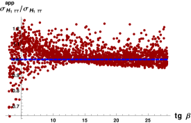
(a)

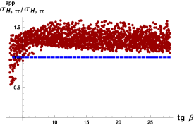
(b)

Figure 4: Comparison of the the approximation to $\sigma(pp\to H_{i}\to\tau\tau)$ in Eq. (4.1.2) with the full result as a function of $\tan\beta$ .

Then the total width is,

$$\Gamma_{i}\gtrsim\frac{g^{2}m_{H_{i}}}{32\pi M_{W}^{2}}\left(\frac{3m_{b}^{2}}{1+\kappa_{d}\tan\beta}+m_{\tau}^{2}\right)\tan^{2}\beta\,,$$ (81)

And thus, the branching ratio is,

$$\mbox{BR}\left(H_{i}\to\tau\tau\right)\lesssim\frac{m_{\tau}^{2}\left(1+\kappa_{d}\tan\beta\right)^{2}}{3m_{b}^{2}+m_{\tau}^{2}\left(1+\kappa_{d}\tan\beta\right)^{2}}$$ (82)

So, for the $\tau\tau$-production cross section of $H_{1}$ and $H_{3}$ we have,

$$\sigma(pp \overset{H_{i}}{\longrightarrow}\tau\tau)\lesssim\frac{\tan^{2}\beta}{\left(1+\kappa_{d}\tan\beta\right)^{2}}\,\frac{m_{\tau}^{2}\left(1+\kappa_{d}\tan\beta\right)^{2}}{3m_{b}^{2}+m_{\tau}^{2}\left(1+\kappa_{d}\tan\beta\right)^{2}}$$

$$\qquad\qquad~{}\left[0.16\left(\frac{\tau_{H_{i}}~{}d{\cal L}^{bb}/d\tau_{H_{i}}}{2300~{}\mbox{pb}}\right)+0.11\left(\frac{\tau_{H_{i}}~{}d{\cal L}^{gg}_{LO}/d\tau_{H_{i}}}{3\times 10^{6}~{}\mbox{pb}}\right)\right]~{}\mbox{pb}$$

$$\simeq \frac{\tan^{2}\beta}{8.4+2\kappa_{d}\tan\beta+\kappa_{d}^{2}\tan^{2}\beta}~{}\left[0.16\left(\frac{\tau_{H_{i}}~{}d{\cal L}^{bb}/d\tau_{H_{i}}}{2300~{}\mbox{pb}}\right)+0.11\left(\frac{\tau_{H_{i}}~{}d{\cal L}^{gg}_{LO}/d\tau_{H_{i}}}{3\times 10^{6}~{}\mbox{pb}}\right)\right]~{}\mbox{pb}$$

which should be compared with the SM cross section $\sigma(pp\to H\to\tau\tau)\simeq 1.4~{}\mbox{pb}$ for $m_{H}\simeq 110$ GeV. The comparison of this approximate expression with the full result is shown in Figure 4. In fact, this approximate expression works very well for $m_{H_{1}}=110$ GeV and is slightly larger than the exact result for $m_{H_{3}}=155$ GeV. This is due to the fact that we did not include the $H_{i}\to WW^{*}$ channel in Eq. (4.1.2) and this channel is important for $H_{3}$, which means that the approximate branching ratio is larger than one in the full expression. Nevertheless, we can safely use this expression to understand the qualitative behaviour in this process.

Next, we combine the bounds on the two photon production cross section and the $\tau\tau$ production cross section in our model with medium-large $\tan\beta$. In Figure 5 we present the $\tau\tau$ production cross sections at LHC for $m_{H_{1}}\simeq 110$ GeV and $m_{H_{3}}\simeq 160$ GeV with (squares in blue) or without (circles in red) fulfilling the requirement $0.75\leq\mu_{\gamma\gamma}^{\rm{LHC}}\leq 1.55$. The green line is the CMS limit on the $\tau\tau$ production cross section for Higgs masses below 150 GeV and the green points are the points where, in addition, the $\tau\tau$ cross-section limit on the observed Higgs, $H_{2}$ in our scenario, at a mass $m_{H_{2}}\simeq 125$ GeV is also fulfilled. Even though we fixed $m_{H_{1}}=110$ GeV in this plot, we have checked that the situation does not change at all for $m_{H_{1}}=100$ GeV or $m_{H_{1}}=120$ GeV.

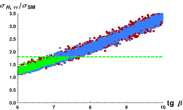
Figure 5: $\tau\tau$ production cross-section at $m_{H_{1}}=110$ GeV as a function of $\tan\beta$, with the CMS limit on $\tau\tau$ production in green.

Notice that, the present constraints on heavy Higgses for $\sigma(pp\to H_{3}\to\tau\tau)$ for masses $150~{}{\rm GeV}\leq m_{H_{3}}\lesssim 200~{}{\rm GeV}$ can only eliminate the region of $\tan\beta\gtrsim 25$, but we expect the future analysis of the stored data to reduce this parameter space significantly privateFiorini .

Hence, we see that there are no points consistent with the LHC constraints on $\sigma(pp\to H_{1}\to\tau\tau)$ for $\tan\beta\geq 7.8$ and $100~{}\mbox{GeV}<m_{H_{1}}<125$ GeV and, as we will see in the next section, all the surviving points are inconsistent with BR($B\to X_{s}\gamma$).

4.2 Low $\tan\beta$ regime.

As we have just seen, LHC constraints on $\sigma(pp\to H_{1}\to\tau\tau)$ rule out the possibility of $m_{H_{2}}\simeq 125$ GeV for $\tan\beta\geq 7.8$, still, the situation for $\tan\beta\lesssim 8$ is very different. For low $\tan\beta$, it is much easier to satisfy the constraint from the $\gamma\gamma$-signal strength at LHC, $\mu_{\gamma\gamma}\gtrsim 0.5$.

Analogously to the discussion in the case of medium-large $\tan\beta$, we can see that the $\gamma\gamma$-decay width for low $\tan\beta$ remains of the same order as the SM one, $\Gamma_{H_{2}\to\gamma\gamma}\simeq\Gamma_{h\to\gamma\gamma}^{SM}$. The production cross section is typically of the order of the SM one, as the $b\bar{b}$-fusion process and the $b$-quark contribution to gluon fusion, being proportional to $\tan\beta$, are now smaller and the top contribution is very close to the SM for ${\cal U}_{22}\simeq O(1)$. In fact, the total decay width is still larger than the SM value if ${\cal U}_{21,21}$ are sizeable, as the $b\bar{b}$ and $\tau\tau$ widths are enhanced by $\tan^{2}\beta$. So, the same requirements on Higgs mixings, Eq. (74), hold true now, although are less suppressed correspondingly to the smaller $\tan\beta$ values. On the other hand, the $\tau\tau$ production cross section through the three neutral Higgses remains an important constraint, but it is much easier to satisfy for low $\tan\beta$ values, as we can see in Fig. 5.

However, in our scenario, we have a rather light charged Higgs, $m_{H^{\pm}}\lesssim 220$ GeV, and the main constraint for $\tan\beta\lesssim 8$ now comes from the $\mbox{BR}(B\rightarrow X_{s}\gamma)$.

4.2.1 Constraints from BR($B\to X_{s}\gamma$)

The decay $B\to X_{s}\gamma$ is an important constraint on the presence of light charged Higgs particles as we have in our scenario. However, although the charged Higgs interferes always constructively with the SM $W$-boson contribution to the Wilson coefficients, in the MSSM this contribution can be compensated by an opposite sign contribution from the stop-chargino loop if $\mbox{Re}\left(\mu A_{t}\right)$ is negative. The charged Higgs contribution is given by Eq. (43). The size of ${\cal C}_{7}^{H^{\pm}}$ can be approximated by the dominant contribution, given by $f_{7}^{(2)}(m^{2}_{t}/m_{H^{\pm}}^{2})$,

$${\cal C}_{7}^{H^{\pm}}\simeq\frac{f_{7}^{(2)}(y_{t})}{1+\delta h_{d}/h_{d}+\Delta h_{d}/h_{d}\tan\beta}\,,$$ (84)

and for $m_{H^{\pm}}\in[150,200]$ GeV we get $f_{7}^{(2)}(y_{t})\in[-0.22,-0.18]$. Incidentally, we see that this charged Higgs contribution decreases with $\tan\beta$, and thus it is more difficult to satisfy the constraints at low $\tan\beta$ unless this contribution is compensated by a different sign contribution. Then for the stop-chargino contribution, using Eq. (3.4.1),

$$\mathcal{C}_{7,8}^{\chi^{\pm}} \simeq -\frac{M_{W}^{2}}{M_{2}^{2}}~{}\frac{M_{2}}{\mu}~{}\tan\beta\left(f_{7,8}^{(3)}\left(x_{\tilde{q}\tilde{\chi}_{1}^{\pm}}\right)-f_{7,8}^{(3)}\left(x_{\tilde{t}_{1}\tilde{\chi}_{1}^{\pm}}\right)\right)$$ (85)

$$- \frac{A_{t}}{\mu}\tan\beta\,\frac{M_{W}^{2}}{M_{2}^{2}}\frac{m_{t}^{2}}{m_{\tilde{t}_{1}}^{2}-m_{\tilde{t}_{2}}^{2}}\>\left(f_{7,8}^{(3)}\left(x_{\tilde{t}_{1}\tilde{\chi}_{1}^{\pm}}\right)-f_{7,8}^{(3)}\left(x_{\tilde{t}_{2}\tilde{\chi}_{1}^{\pm}}\right)\right)$$

Taking now $f_{7}^{(3)}\left(x\simeq 1\right)\simeq 0.44$, and therefore, with the limits on stop and chargino masses, $m_{\tilde{t}_{1}}\geq 650$ GeV and $m_{\chi^{\pm}}\geq 350$ GeV, we estimate $\mathcal{C}_{7}^{\chi^{\pm}}\simeq 0.02~{}M_{2}/\mu~{}\tan\beta\ll{\cal C}_{7,8}^{H^{\pm}}$. Thus it looks very difficult to compensate the charged Higgs contribution for low $\tan\beta$ and this is confirmed in the numerical analysis.

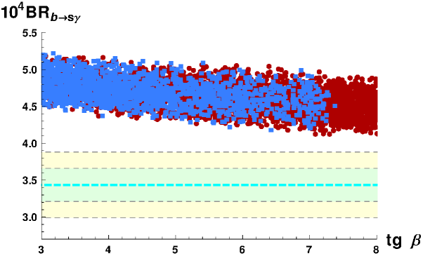
Figure 6: Branching ratio of the $B\to X_{s}\gamma$ decay as a function of $\tan\beta$. Blue squares fulfil the $\mu^{\rm LHC}_{\gamma\gamma}$ and $\sigma_{H_{i}\tau\tau}/\sigma_{\rm SM}$ constraints, as explained in the text. Green and yellow regions are the one and two-$\sigma$ experimentally allowed regions.

In Figure 6, we present the obtained BR($B\to X_{s}\gamma$), the blue squares fulfil the requirements of, $0.75\leq\mu^{\rm LHC}_{\gamma\gamma}\leq 1.55$, $\sigma_{H_{1}\tau\tau}/\sigma_{\rm SM}\leq 1.8$ and $\sigma_{H_{2}\tau\tau}/\sigma_{\rm SM}\leq 1.8$ while the red dots violate some of these requirements. The experimentally allowed region at the one-$\sigma$ and two-$\sigma$ level is shown in green and yellow respectively . In passing, please note that the reduction of the BR with $\tan\beta$ is mainly due to the reduction of the charged Higgs contribution, as shown in Eq. (84), and not to the negative interference with the chargino diagram.

Therefore, the only remaining option is to have a light stop with a small mass difference with respect to the lightest neutralino that has escaped detection so far at LHC. To explore numerically this possibility, we select the lightest stop mass to be $m_{\chi^{0}_{1}}\leq m_{\tilde{t}_{1}}\leq m_{t}+m_{\chi^{0}_{1}}$. The result is shown in Fig. 7, where we plot again BR($B\to X_{s}\gamma$) as a function of $\tan\beta$.

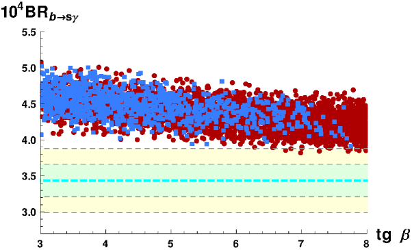
Figure 7: Branching ratio of the $B\to X_{s}\gamma$ decay as a function of $\tan\beta$, for $m_{\tilde{t}_{1}}\leq 650$ and $m_{\chi^{0}_{1}}\leq m_{\tilde{t}_{1}}\leq m_{t}+m_{\chi^{0}_{1}}$. The color coding is the same as in Fig. 6

Now, we can see that the range of BR($B\to X_{s}\gamma$) for a given $\tan\beta$ has decreased, as expected, due to a possible destructive interference of the stop-chargino diagram. Nevertheless, we can see that there are no points allowed by collider constraints that reach the two-$\sigma$ allowed region.

As a by-product, we can already see from here that it will be very difficult, if not completely impossible, to accommodate two sizeable Higgs-like peaks in the $\gamma\gamma$ production cross section, as recently announced by the CMS collaboration CMS-PAS-HIG-13-016 , within an MSSM context. The CMS analysis of an integrated luminosity of 5.1 (19.6) fb^-1 at a center of mass energy of 7 (8) TeV reveals a clear excess near $m_{H}=136.5$ GeV, aside from the 125–126 GeV Higgs boson that has already been discovered, with a local significance for this extra peak of 2.73 $\sigma$ combining the data from Higgs coming from vector-boson fusion and vector-boson associated production (each of which shows the excess individually).

As we have shown in this work, the  125 GeV Higgs found at the LHC ought to be the lightest, therefore this new resonance, despite its light mass, is bounded to be the second lightest Higgs, meaning that the third neutral Higgs (and its charged sibling) are to be found nearby. This can be easily seen following our line of reasoning in section 3, where we obtain $m_{H_{3}}<180$ GeV and $m_{H^{+}}<200$ GeV. However, to reproduce the observed signal strength in $H_{1}\longrightarrow\gamma\gamma$ of the $\sim 126$ GeV peak for medium–large $\tan\beta$, we must force all the pseudoscalar and down-type content out of the lightest state. In this case, we have ${\cal U}_{12}\approx 1$ and ${\cal U}_{11},{\cal U}_{13}\ll 1$, so that the the two heavier Higgses will necessarily couple, with $\tan\beta$-enhancement, to down-type fermions and the branching ratio of these Higgses to $\gamma\gamma$ will be brutally inhibited. At the same time, the $H_{i}\longrightarrow\tau\tau$ channel, for $i=2,3$ is $\propto(U_{i1}^{2}+U_{i3}^{2})\approx(1-U_{i2}^{2})\approx U_{12}^{2}\simeq 1$. Meaning that any MSSM setting would predict a $H_{i}\longrightarrow\tau\tau$ at a level that is already excluded Aad:2012mea ; CMS-PAS-HIG-13-004 ; Aad:2012yfa .

The only possible escape to this situation would be to stay in the (very) low $\tan\beta$ region, but then, given the low mass of the charged Higgs, the constraints from BR($B\to X_{s}\gamma$) eliminate completely this possibility. Therefore, we can not see any way to accommodate two Higgs peaks in the $\gamma\gamma$ spectrum with a signal strength of the order of the SM model one. Nevertheless this possibility will be fully explored in a subsequent paper WIP .

5 Conclusions.

In this work we have investigated the possibility of the Higgs found at LHC with a mass $m_{H}\sim 125$ GeV not being the lightest but the second lightest Higgs in an MSSM context, having the actual lightest Higgs escaped detection due to its pseudoscalar and/or down-type content. In this scheme, such a content suppresses simultaneously its couplings to gauge bosons and up-type quarks and paves the way to evade LEP constraints.

Although similar studies, with previous LHC constraints, are already present in the literature, most of these studies proceed through giant scans of the model’s parameter space and the later analysis of the scanning results. Our approach in this work has been different, and we have chosen to study analytically, with simple expressions under reasonable approximations, three or four key phenomenological signatures, including the two photon signal strength and the $\tau\tau$ production cross sections at LHC and the indirect constraints on BR$(B\to X_{s}\gamma)$. To the best of our knowledge, this is the first study carried out in this way in an MSSM context using the LHC data. Our approach has the advantage that can rule out the model altogether without risking having missed a region where unexpected cancellations or combinations can take place.

This analysis is accomplished in a completely generic MSSM, in terms of SUSY parameters at the electroweak scale, such that it encloses all possible MSSM setups. To be as general as possible, we have allowed for the presence of CP violating phases in the Higgs potential such that the three neutral-Higgs eigenstates become admixtures with no definite CP–parity. Our study starts with the $\gamma\gamma$ signal observed at LHC at $m_{H}\simeq 125$ GeV. The experimental results show a signal slightly larger or of the order of the SM expectations, and this is a strong constraint on models with extended Higgs sectors. We have shown than in the MSSM with $m_{H_{2}}\simeq 125$ GeV the width $\Gamma(H_{2}\to\gamma\gamma)$ cannot be substantially modified from its SM value. On the other hand, the total width of $H_{2}$ tends to be significantly larger if the down-type or pseudoscalar components of $H_{2}$ are sizeable. Simply requiring that BR$(H_{2}\to\gamma\gamma)$ or, more exactly, $\sigma(pp\to H_{2})\times\mbox{BR}(H_{2}\to\gamma\gamma)$ is not much smaller than the SM severely restricts the possible mixings in the Higgs sector and determines the bottom and $\tau$ decay rates of the three Higgses.

Next, we have analyzed the $\tau\tau$ production cross sections for the three Higgs eigenstates, splitting the parameter space in two regions of large and small $\tan\beta$, being the dividing line $\tan\beta\simeq 8$. We have shown that, for large $\tan\beta$, present constraints on $\sigma(pp\to H_{1}\to\tau\tau)$ forbid all points in the model parameter space irrespective of the supersymmetric mass spectrum.

On the other hand, in the low $\tan\beta$ region, the presence of a relatively light charged Higgs, $m_{H^{\pm}}\lesssim 220$ GeV, provides a large charged-Higgs contribution to $\mbox{BR}(B\to X_{s}\gamma)$ which can not be compensated by an opposite sign chargino contribution, precisely due to the smallness of $\tan\beta$ and this eliminates completely the possibility of the observed Higgs at $M_{H}\simeq 125$ GeV, being the next-to-lightest Higgs in an MSSM context.

In summary, we have shown that a carefully chosen combination of three or four experimental signatures can be enough to entirely rule out a model without resorting to gigantic scans while simultaneously provides a much better understanding on the physics of the model studied. The power of this technique should not be underestimated specially when studying models with large parameter spaces where monster scans can be quite time consuming and not precisely enlightening. Special interest raises the case in which the Higgs found at the LHC is the lightest where this type of combined analysis can close significant regions of the parameters space WIP .

In this respect, the straightforward application of this kind of study to the recently published CMS data with a second Higgs-like resonance at $\sim 136$ GeV, aside from the 125–126 GeV Higgs, shows it is not possible to accommodate both resonances in the $\gamma\gamma$ spectrum with a signal strength of the order of the SM model one.

Appendix A MSSM Conventions

We follow the MSSM conventions in the classical review of Haber and Kane Haber:1984rc , see also Chung:2003fi . In this section we review the mass matrices entering in our analysis,

Charginos:

In our convention the chargino mass matrix is,

$$\mathcal{M}_{C}=\left(\begin{array}[]{cc}M_{2}&\sqrt{2}M_{W}\sin\beta\\ \sqrt{2}M_{W}\cos\beta&\mu\end{array}\right)$$ (86)

and can be diagonalized by two unitary matrices so that $U^{*}\mathcal{M}_{C}V^{\dagger}=\mbox{Diag.}\left\{m_{\chi_{1}^{\pm}},\>m_{\chi_{2}^{\pm}}\right\}$ with $m_{\chi_{1}^{\pm}}\leq m_{\chi_{2}^{\pm}}$. The mass eigenstates, $\chi_{i}^{\pm}$, are related to the electroweak eigenstates, $\hat{\chi}_{i}^{\pm}$, by

$$\chi_{i}^{+}=V_{ij}\hat{\chi}_{j}^{+}\,,\qquad\chi_{i}^{-}=U_{ij}\hat{\chi}_{j}^{-}\,.$$ (87)

Sfermions:

The squark mass matrix is given by,

$$\mathcal{M}_{q}^{2}=\left(\begin{array}[]{cc}M_{\tilde{Q}_{3}}^{2}+m_{q}^{2}+\cos\left(2\beta\right)M_{Z}^{2}\left(R_{z}^{q}-Q_{q}\sin^{2}\theta_{W}\right)&h_{q}^{*}\upsilon_{q}\left(A_{q}^{*}-\mu T_{q}\right)/\sqrt{2}\\ \\ h_{q}\upsilon_{q}\left(A_{q}-\mu^{*}T_{q}\right)/\sqrt{2}&M_{\tilde{R}_{3}}^{2}+m_{q}^{2}+\cos\left(2\beta\right)M_{Z}^{2}Q_{q}\sin^{2}\theta_{W}\end{array}\right)$$ (88)

With $R_{z}^{t}=-R_{z}^{b}=\frac{1}{2}$, $Q_{q}$ the quark charge, $T_{b}=\tan\beta=\frac{\upsilon_{u}}{\upsilon_{d}}=T_{t}^{-1}$ and $h_{q}$ the Yukawa coupling corresponding to the quark. This matrix is diagonalized ${\cal R}_{q}\mathcal{M}_{\tilde{q}}^{2}{\cal R}_{q}^{\dagger}=\mbox{Diag.}\left\{m_{\tilde{q}_{1}}^{2},\>m_{\tilde{q}_{2}}^{2}\right\}$

Similarly, the stau mass matrix,

$$\mathcal{M}_{\tau}^{2}=\left(\begin{array}[]{cc}M_{\tilde{L}_{3}}^{2}+m_{\tau}^{2}+\cos\left(2\beta\right)M_{Z}^{2}\left(\sin^{2}\theta_{W}-\frac{1}{2}\right)&h_{\tau}^{*}\upsilon_{1}\left(A_{\tau}^{*}-\mu\tan\beta\right)/\sqrt{2}\\ \\ h_{\tau}\upsilon_{1}\left(A_{\tau}-\mu^{*}\tan\beta\right)/\sqrt{2}&M_{\tilde{E}_{3}}^{2}+m_{\tau}^{2}+\cos\left(2\beta\right)M_{Z}^{2}\sin^{2}\theta_{W}\end{array}\right)$$ (89)

Appendix B Expansion of Hermitian matrices

Following Refs. Buras:1997ij ; Masiero:2005ua , we have that given a $n\times n$ hermitian matrix $A=A^{0}+A^{1}$ with $A^{0}=Diag(a_{1}^{0},...,a_{n}^{0})$ and $A^{1}$completely off diagonal that is diagonalized by $\mathcal{U}\cdot A\cdot\mathcal{U}^{\dagger}=Diag(a_{1},...,a_{n})$, we have a first order in $A^{1}$:

$$\mathcal{U}_{ki}^{*}f\left(a_{k}\right)\mathcal{U}_{kj}\simeq\delta_{ij}f(a_{i}^{0})+A_{ij}^{1}\frac{f(a_{i}^{0})-f(a_{j}^{0})}{a_{i}^{0}-a_{j}^{0}}$$ (90)

We use this formula to expand the chargino Wilson coefficients, ${\cal C}_{7,8}$, with respect to the chargino mass matrix elements. In this case we have to be careful because the chargino mass matrix is not hermitian. However due to the necessary chirality flip in the chargino line ${\cal C}_{7,8}$ is a function of odd powers of $M_{\chi^{+}}$ Clavelli:2000ua , and then

$$\sum_{j=1}^{2}U_{j2}V_{j1}m_{\chi_{j}^{+}}A(m_{\chi_{j}^{+}}^{2})=\sum_{j,k,l=1}^{2}U_{jk}m_{\chi_{j}^{+}}V_{j1}U_{l2}A(m_{\chi_{l}^{+}}^{2})U_{lk}^{*}$$ (91)

where we introduced $\sum_{k}U_{jk}U_{lk}^{*}=\delta_{jl}$. Then, we obtain,

$$\mathcal{C}_{7,8}^{\chi^{\pm}(a)} = \frac{1}{\cos\beta}\sum_{{\scriptstyle a=1,2}}\frac{U_{a2}V_{a1}M_{W}}{\sqrt{2}m_{\tilde{\chi}_{a}^{\pm}}}\mathcal{F}_{7,8}\left(x_{\tilde{q}\tilde{\chi}_{a}^{\pm}},x_{\tilde{t}_{1}\tilde{\chi}_{a}^{\pm}},x_{\tilde{t}_{2}\tilde{\chi}_{a}^{\pm}}\right)$$

$$\sim \frac{M_{W}}{\sqrt{2}\cos\beta}\left[~{}\left(\mathcal{M}_{\chi}\right)_{21}\frac{\mathcal{F}_{7,8}\left(x_{\tilde{q}\tilde{\chi}_{2}^{\pm}},x_{\tilde{t}_{1}\tilde{\chi}_{2}^{\pm}},x_{\tilde{t}_{2}\tilde{\chi}_{2}^{\pm}}\right)}{m_{\tilde{\chi}_{2}^{\pm}}^{2}}\right.$$

$$+ \left.\left(\mathcal{M}_{\chi}\right)_{11}\left(\mathcal{M}_{\chi}\mathcal{M}_{\chi}^{\dagger}\right)_{21}\frac{m_{\tilde{\chi}_{1}^{\pm}}^{2}\mathcal{F}_{7,8}\left(x_{\tilde{q}\tilde{\chi}_{2}^{\pm}},x_{\tilde{t}_{1}\tilde{\chi}_{2}^{\pm}},x_{\tilde{t}_{2}\tilde{\chi}_{2}^{\pm}}\right)-m_{\tilde{\chi}_{2}^{\pm}}^{2}\mathcal{F}_{7,8}\left(x_{\tilde{q}\tilde{\chi}_{1}^{\pm}},x_{\tilde{t}_{1}\tilde{\chi}_{1}^{\pm}},x_{\tilde{t}_{2}\tilde{\chi}_{1}^{\pm}}\right)}{m_{\tilde{\chi}_{1}^{\pm}}^{2}m_{\tilde{\chi}_{2}^{\pm}}^{2}\left(m_{\tilde{\chi}_{2}^{\pm}}^{2}-m_{\tilde{\chi}_{1}^{\pm}}^{2}\right)}\right];$$

$$\mathcal{C}_{7,8}^{\chi^{\pm}(b)} = \frac{1}{\cos\beta}\sum_{{\scriptstyle a=1,2}}\frac{U_{a2}V_{a2}\overline{m}_{t}}{2m_{\tilde{\chi}_{a}^{\pm}}\sin\beta}\mathcal{G}_{7,8}\left(x_{\tilde{t}_{1}\tilde{\chi}_{a}^{\pm}},x_{\tilde{t}_{2}\tilde{\chi}_{a}^{\pm}}\right)$$

$$\sim \frac{\overline{m}_{t}}{2\cos\beta\sin\beta}\left[~{}\left(\mathcal{M}_{\chi}\right)_{22}\frac{\mathcal{G}_{7,8}\left(x_{\tilde{q}\tilde{\chi}_{2}^{\pm}},x_{\tilde{t}_{1}\tilde{\chi}_{2}^{\pm}},x_{\tilde{t}_{2}\tilde{\chi}_{2}^{\pm}}\right)}{m_{\tilde{\chi}_{2}^{\pm}}^{2}}\right.$$

$$+ \left.\left(\mathcal{M}_{\chi}\right)_{12}\left(\mathcal{M}_{\chi}\mathcal{M}_{\chi}^{\dagger}\right)_{21}\frac{m_{\tilde{\chi}_{1}^{\pm}}^{2}\mathcal{G}_{7,8}\left(x_{\tilde{q}\tilde{\chi}_{2}^{\pm}},x_{\tilde{t}_{1}\tilde{\chi}_{2}^{\pm}},x_{\tilde{t}_{2}\tilde{\chi}_{2}^{\pm}}\right)-m_{\tilde{\chi}_{2}^{\pm}}^{2}\mathcal{G}_{7,8}\left(x_{\tilde{q}\tilde{\chi}_{1}^{\pm}},x_{\tilde{t}_{1}\tilde{\chi}_{1}^{\pm}},x_{\tilde{t}_{2}\tilde{\chi}_{1}^{\pm}}\right)}{m_{\tilde{\chi}_{1}^{\pm}}^{2}m_{\tilde{\chi}_{2}^{\pm}}^{2}\left(m_{\tilde{\chi}_{2}^{\pm}}^{2}-m_{\tilde{\chi}_{1}^{\pm}}^{2}\right)}\right];$$

and using again the same approximation we can expand the stop mixings in the ${\cal F}_{7,8}$ and ${\cal G}_{7,8}$, we obtain:

$$\mathcal{F}_{7,8}\left(x_{\tilde{q}\tilde{\chi}_{a}^{\pm}},x_{\tilde{t}_{1}\tilde{\chi}_{a}^{\pm}},x_{\tilde{t}_{2}\tilde{\chi}_{a}^{\pm}}\right) \simeq f_{7,8}^{(3)}\left(x_{\tilde{q}\tilde{\chi}_{a}^{\pm}}\right)-f_{7,8}^{(3)}\left(x_{\tilde{t}_{1}\tilde{\chi}_{a}^{\pm}}\right);$$ (94)

$$\mathcal{G}_{7,8}\left(x_{\tilde{t}_{1}\tilde{\chi}_{a}^{\pm}},x_{\tilde{t}_{2}\tilde{\chi}_{a}^{\pm}}\right) \simeq \left(\mathcal{M}_{\tilde{t}}\right)_{21}\frac{f_{7,8}^{(3)}\left(x_{\tilde{t}_{1}\tilde{\chi}_{a}^{\pm}}\right)-f_{7,8}^{(3)}\left(x_{\tilde{t}_{2}\tilde{\chi}_{a}^{\pm}}\right)}{m_{\tilde{t}_{1}}^{2}-m_{\tilde{t}_{2}}^{2}};$$ (95)

So, putting all together, we have:

$$\mathcal{C}_{7,8}^{\chi^{\pm}(a)} \sim \frac{M_{W}}{\sqrt{2}\cos\beta}\left[~{}\left(\mathcal{M}_{\chi}\right)_{21}\frac{f_{7,8}^{(3)}\left(x_{\tilde{q}\tilde{\chi}_{2}^{\pm}}\right)-f_{7,8}^{(3)}\left(x_{\tilde{t}_{1}\tilde{\chi}_{2}^{\pm}}\right)}{m_{\tilde{\chi}_{2}^{\pm}}^{2}}\right.$$

$$+ \left.\frac{\left(\mathcal{M}_{\chi}\right)_{11}\left(\mathcal{M}_{\chi}\mathcal{M}_{\chi}^{\dagger}\right)_{21}}{m_{\tilde{\chi}_{1}^{\pm}}^{2}-m_{\tilde{\chi}_{2}^{\pm}}^{2}}\left(\frac{f_{7,8}^{(3)}\left(x_{\tilde{q}\tilde{\chi}_{1}^{\pm}}\right)-f_{7,8}^{(3)}\left(x_{\tilde{t}_{1}\tilde{\chi}_{1}^{\pm}}\right)}{m_{\tilde{\chi}_{1}^{\pm}}^{2}}-\frac{f_{7,8}^{(3)}\left(x_{\tilde{q}\tilde{\chi}_{2}^{\pm}}\right)-f_{7,8}^{(3)}\left(x_{\tilde{t}_{1}\tilde{\chi}_{2}^{\pm}}\right)}{m_{\tilde{\chi}_{2}^{\pm}}^{2}}\right)\right];$$

$$\mathcal{C}_{7,8}^{\chi^{\pm}(b)} \sim \frac{\overline{m}_{t}}{2\cos\beta\sin\beta}\left[~{}\left(\mathcal{M}_{\chi}\right)_{22}\frac{\left(\mathcal{M}_{\tilde{t}}\right)_{21}}{m_{\tilde{t}_{1}}^{2}-m_{\tilde{t}_{2}}^{2}}\left(\frac{f_{7,8}^{(3)}\left(x_{\tilde{t}_{1}\tilde{\chi}_{2}^{\pm}}\right)-f_{7,8}^{(3)}\left(x_{\tilde{t}_{2}\tilde{\chi}_{2}^{\pm}}\right)}{m_{\tilde{\chi}_{2}^{\pm}}^{2}}\right)\right.$$

$$+ \left.\frac{\left(\mathcal{M}_{\chi}\right)_{12}\left(\mathcal{M}_{\chi}\mathcal{M}_{\chi}^{\dagger}\right)_{21}}{m_{\tilde{\chi}_{1}^{\pm}}^{2}-m_{\tilde{\chi}_{2}^{\pm}}^{2}}\left(\frac{f_{7,8}^{(3)}\left(x_{\tilde{t}_{1}\tilde{\chi}_{1}^{\pm}}\right)-f_{7,8}^{(3)}\left(x_{\tilde{t}_{2}\tilde{\chi}_{1}^{\pm}}\right)}{m_{\tilde{\chi}_{1}^{\pm}}^{2}}-\frac{f_{7,8}^{(3)}\left(x_{\tilde{t}_{1}\tilde{\chi}_{2}^{\pm}}\right)-f_{7,8}^{(3)}\left(x_{\tilde{t}_{2}\tilde{\chi}_{2}^{\pm}}\right)}{m_{\tilde{\chi}_{2}^{\pm}}^{2}}\right)\right.$$

$$\left.\frac{\left(\mathcal{M}_{\tilde{t}}\right)_{21}}{m_{\tilde{t}_{1}}^{2}-m_{\tilde{t}_{2}}^{2}}\right];$$

References

- (1) G. Aad et al. [ATLAS Collaboration], Phys. Lett. B 716, 1 (2012) [arXiv:1207.7214 [hep-ex]].
- (2) S. Chatrchyan et al. [CMS Collaboration], Phys. Lett. B 716, 30 (2012) [arXiv:1207.7235 [hep-ex]].
- (3) S. R. Coleman and J. Mandula, Phys. Rev. 159, 1251 (1967).
- (4) R. Haag, J. T. Lopuszanski and M. Sohnius, Nucl. Phys. B 88, 257 (1975).
- (5) P. Fayet, Nucl. Phys. B 90, 104 (1975).
- (6) P. Fayet, Phys. Lett. B 69, 489 (1977).
- (7) G. R. Farrar and P. Fayet, Phys. Lett. B 76, 575 (1978).
- (8) E. Witten, Nucl. Phys. B 188, 513 (1981).
- (9) S. Dimopoulos and H. Georgi, Nucl. Phys. B 193, 150 (1981).
- (10) N. Sakai, Z. Phys. C 11, 153 (1981).
- (11) L. E. Ibanez and G. G. Ross, Phys. Lett. B 105, 439 (1981).
- (12) R. K. Kaul, Phys. Lett. B 109, 19 (1982).
- (13) H. P. Nilles, Phys. Rept. 110, 1 (1984).
- (14) H. E. Haber and G. L. Kane, Phys. Rept. 117, 75 (1985).
- (15) A. Djouadi, Phys. Rept. 459, 1 (2008) [hep-ph/0503173].
- (16) A. Pilaftsis, Phys. Lett. B 435, 88 (1998) [hep-ph/9805373].
- (17) A. Pilaftsis, Phys. Rev. D 58, 096010 (1998) [hep-ph/9803297].
- (18) A. Pilaftsis and C. E. M. Wagner, Nucl. Phys. B 553, 3 (1999) [hep-ph/9902371].
- (19) D. A. Demir, Phys. Rev. D 60, 055006 (1999) [hep-ph/9901389].
- (20) M. S. Carena, J. R. Ellis, A. Pilaftsis and C. E. M. Wagner, Nucl. Phys. B 586, 92 (2000) [hep-ph/0003180].
- (21) S. Y. Choi, M. Drees and J. S. Lee, Phys. Lett. B 481, 57 (2000) [hep-ph/0002287].
- (22) M. S. Carena, J. R. Ellis, A. Pilaftsis and C. E. M. Wagner, Nucl. Phys. B 625, 345 (2002) [hep-ph/0111245].
- (23) S. Y. Choi, K. Hagiwara and J. S. Lee, Phys. Rev. D 64, 032004 (2001) [hep-ph/0103294].
- (24) S. Y. Choi, M. Drees, J. S. Lee and J. Song, Eur. Phys. J. C 25, 307 (2002) [hep-ph/0204200].
- (25) S. M. Barr and A. Zee, Phys. Rev. Lett. 65, 21 (1990) [Erratum-ibid. 65, 2920 (1990)].
- (26) D. Chang, W. -F. Chang and W. -Y. Keung, Phys. Lett. B 478, 239 (2000) [hep-ph/9910465].
- (27) J. R. Ellis, J. S. Lee and A. Pilaftsis, JHEP 0810, 049 (2008) [arXiv:0808.1819 [hep-ph]].
- (28) A. Pilaftsis, Phys. Lett. B 471, 174 (1999) [hep-ph/9909485].
- (29) S. Heinemeyer, O. Stal and G. Weiglein, Phys. Lett. B 710, 201 (2012) [arXiv:1112.3026 [hep-ph]].
- (30) K. Hagiwara, J. S. Lee and J. Nakamura, JHEP 1210, 002 (2012) [arXiv:1207.0802 [hep-ph]].
- (31) A. Arbey, M. Battaglia, A. Djouadi and F. Mahmoudi, JHEP 1209, 107 (2012) [arXiv:1207.1348 [hep-ph]].
- (32) P. Bechtle, S. Heinemeyer, O. Stal, T. Stefaniak, G. Weiglein and L. Zeune, Eur. Phys. J. C 73, 2354 (2013) [arXiv:1211.1955 [hep-ph]].
- (33) J. Ke, H. Luo, M. -x. Luo, K. Wang, L. Wang and G. Zhu, Phys. Lett. B 723, 113 (2013) [arXiv:1211.2427 [hep-ph]].
- (34) J. Ke, H. Luo, M. -x. Luo, T. -y. Shen, K. Wang, L. Wang and G. Zhu, arXiv:1212.6311 [hep-ph].
- (35) S. Moretti, S. Munir and P. Poulose, arXiv:1305.0166 [hep-ph].
- (36) S. Scopel, N. Fornengo and A. Bottino, arXiv:1304.5353 [hep-ph].
- (37) J. S. Lee, A. Pilaftsis, M. S. Carena, S. Y. Choi, M. Drees, J. R. Ellis and C. E. M. Wagner, Comput. Phys. Commun. 156, 283 (2004) [hep-ph/0307377].
- (38) J. S. Lee, M. Carena, J. Ellis, A. Pilaftsis and C. E. M. Wagner, Comput. Phys. Commun. 184, 1220 (2013) [arXiv:1208.2212 [hep-ph]].
- (39) S. Heinemeyer, W. Hollik and G. Weiglein, Comput. Phys. Commun. 124, 76 (2000) [hep-ph/9812320].
- (40) T. Hahn, W. Hollik, S. Heinemeyer and G. Weiglein, eConf C 050318, 0106 (2005) [hep-ph/0507009].
- (41) J. R. Ellis, K. A. Olive and Y. Santoso, Phys. Lett. B 539, 107 (2002) [hep-ph/0204192].
- (42) J. R. Ellis, T. Falk, K. A. Olive and Y. Santoso, Nucl. Phys. B 652, 259 (2003) [hep-ph/0210205].
- (43) J. R. Ellis, K. A. Olive and P. Sandick, Phys. Rev. D 78, 075012 (2008) [arXiv:0805.2343 [hep-ph]].
- (44) C. F. Berger, J. S. Gainer, J. L. Hewett and T. G. Rizzo, JHEP 0902, 023 (2009) [arXiv:0812.0980 [hep-ph]].
- (45) S. S. AbdusSalam, B. C. Allanach, F. Quevedo, F. Feroz and M. Hobson, Phys. Rev. D 81, 095012 (2010) [arXiv:0904.2548 [hep-ph]].
- (46) A. Arbey, M. Battaglia, A. Djouadi and F. Mahmoudi, Phys. Lett. B 720, 153 (2013) [arXiv:1211.4004 [hep-ph]].
- (47) [ATLAS Collaboration], ATLAS-CONF-2013-034.
- (48) [CMS Collaboration], CMS-PAS-HIG-13-005.
- (49) G. Aad et al. [ATLAS Collaboration], arXiv:1307.1427 [hep-ex].
- (50) G. Aad et al. [ATLAS Collaboration], JHEP 1209, 070 (2012) [arXiv:1206.5971 [hep-ex]].
- (51) [CMS Collaboration], CMS-PAS-HIG-13-004.
- (52) G. Aad et al. [ATLAS Collaboration], JHEP 1302, 095 (2013) [arXiv:1211.6956 [hep-ex]].
- (53) L. Fiorini, private communication.
- (54) G. Aad et al. [ATLAS Collaboration], JHEP 1206, 039 (2012) [arXiv:1204.2760 [hep-ex]].
- (55) [CMS Collaboration], CMS-PAS-HIG-12-052
- (56) S. Chatrchyan et al. [CMS Collaboration], JHEP 1303, 037 (2013) [arXiv:1212.6194 [hep-ex]].
- (57) S. Chatrchyan et al. [CMS Collaboration], arXiv:1305.2390 [hep-ex].
- (58) [CMS Collaboration], PAS-SUS-13-007
- (59) [CMS Collaboration], PAS-SUS-13-008
- (60) [ATLAS Collaboration], ATLAS-CONF-2012-145.
- (61) [ATLAS Collaboration], ATLAS-CONF-2013-007.
- (62) S. Chatrchyan et al. [CMS Collaboration], arXiv:1303.2985 [hep-ex].
- (63) [ATLAS Collaboration], ATLAS-CONF-2013-024.
- (64) [ATLAS Collaboration], ATLAS-CONF-2013-037.
- (65) [ATLAS Collaboration], ATLAS-CONF-2013-053
- (66) [CMS Collaboration], PAS-SUS-13-011
- (67) [ATLAS Collaboration], ATLAS-CONF-2013-035.
- (68) [CMS Collaboration], PAS-SUS-12-022
- (69) A. Bharucha, S. Heinemeyer and F. von der Pahlen, arXiv:1307.4237 [hep-ph].
- (70) A. Masiero and O. Vives, Ann. Rev. Nucl. Part. Sci. 51, 161 (2001) [hep-ph/0104027].
- (71) M. Raidal, A. van der Schaaf, I. Bigi, M. L. Mangano, Y. K. Semertzidis, S. Abel, S. Albino and S. Antusch et al., Eur. Phys. J. C 57, 13 (2008) [arXiv:0801.1826 [hep-ph]].
- (72) L. Calibbi, R. N. Hodgkinson, J. Jones Perez, A. Masiero and O. Vives, Eur. Phys. J. C 72, 1863 (2012) [arXiv:1111.0176 [hep-ph]].
- (73) RAaij et al. [LHCb Collaboration], Phys. Rev. Lett. 110, 021801 (2013) [arXiv:1211.2674 [hep-ex]].
- (74) RAaij et al. [LHCb Collaboration], Phys. Rev. Lett. 111, 101805 (2013) [arXiv:1307.5024 [hep-ex]].
- (75) S. Chatrchyan et al. [CMS Collaboration], arXiv:1307.5025 [hep-ex].
- (76) S. Chen et al. [CLEO Collaboration], Phys. Rev. Lett. 87, 251807 (2001) [hep-ex/0108032].
- (77) K. Abe et al. [Belle Collaboration], Phys. Lett. B 511, 151 (2001) [hep-ex/0103042].
- (78) A. Limosani et al. [Belle Collaboration], Phys. Rev. Lett. 103, 241801 (2009) [arXiv:0907.1384 [hep-ex]].
- (79) J. P. Lees et al. [BaBar Collaboration], Phys. Rev. D 86, 052012 (2012) [arXiv:1207.2520 [hep-ex]].
- (80) J. P. Lees et al. [BaBar Collaboration], Phys. Rev. D 86, 112008 (2012) [arXiv:1207.5772 [hep-ex]].
- (81) B. Aubert et al. [BaBar Collaboration], Phys. Rev. D 77, 051103 (2008) [arXiv:0711.4889 [hep-ex]].
- (82) Y. Amhis et al. [Heavy Flavor Averaging Group Collaboration], arXiv:1207.1158 [hep-ex].
- (83) HFAG: Rare B decay parameterss, http://www.slac.stanford.edu/xorg/hfag/rare/
- (84) K. Funakubo, S. Tao and F. Toyoda, Prog. Theor. Phys. 109, 415 (2003) [hep-ph/0211238].
- (85) Y. Okada, M. Yamaguchi and T. Yanagida, Prog. Theor. Phys. 85, 1 (1991).
- (86) J. R. Ellis, G. Ridolfi and F. Zwirner, Phys. Lett. B 257, 83 (1991).
- (87) H. E. Haber and R. Hempfling, Phys. Rev. Lett. 66, 1815 (1991).
- (88) H. E. Haber, R. Hempfling and A. H. Hoang, Z. Phys. C 75 (1997) 539 [hep-ph/9609331].
- (89) A. Djouadi and J. Quevillon, arXiv:1304.1787 [hep-ph].
- (90) M. S. Carena, J. R. Espinosa, M. Quiros and C. E. M. Wagner, Phys. Lett. B 355, 209 (1995) [hep-ph/9504316].
- (91) M. S. Carena, J. R. Ellis, A. Pilaftsis and C. E. M. Wagner, Phys. Lett. B 495 (2000) 155 [hep-ph/0009212].
- (92) M. S. Carena, J. R. Ellis, S. Mrenna, A. Pilaftsis and C. E. M. Wagner, Nucl. Phys. B 659, 145 (2003) [hep-ph/0211467].
- (93) K. E. Williams and G. Weiglein, Phys. Lett. B 660, 217 (2008) [arXiv:0710.5320 [hep-ph]].
- (94) L. J. Hall, R. Rattazzi and U. Sarid, Phys. Rev. D 50, 7048 (1994) [hep-ph/9306309].
- (95) M. S. Carena, M. Olechowski, S. Pokorski and C. E. M. Wagner, Nucl. Phys. B 426, 269 (1994) [hep-ph/9402253].
- (96) T. Blazek, S. Raby and S. Pokorski, Phys. Rev. D 52, 4151 (1995) [hep-ph/9504364].
- (97) M. S. Carena, D. Garcia, U. Nierste and C. E. M. Wagner, Nucl. Phys. B 577, 88 (2000) [hep-ph/9912516].
- (98) C. Hamzaoui, M. Pospelov and M. Toharia, Phys. Rev. D 59, 095005 (1999) [hep-ph/9807350].
- (99) K. S. Babu and C. F. Kolda, Phys. Rev. Lett. 84, 228 (2000) [hep-ph/9909476].
- (100) G. Isidori and A. Retico, JHEP 0111, 001 (2001) [hep-ph/0110121].
- (101) A. Dedes and A. Pilaftsis, Phys. Rev. D 67, 015012 (2003) [hep-ph/0209306].
- (102) A. J. Buras, P. H. Chankowski, J. Rosiek and L. Slawianowska, Nucl. Phys. B 659, 3 (2003) [hep-ph/0210145].
- (103) M. Spira, A. Djouadi, D. Graudenz and P. M. Zerwas, Nucl. Phys. B 453, 17 (1995) [hep-ph/9504378].
- (104) M. Spira, Fortsch. Phys. 46, 203 (1998) [hep-ph/9705337].
- (105) A. Djouadi, Phys. Rept. 457, 1 (2008) [hep-ph/0503172].
- (106) A. Dedes and S. Moretti, Phys. Rev. Lett. 84, 22 (2000) [hep-ph/9908516].
- (107) A. Dedes and S. Moretti, Nucl. Phys. B 576, 29 (2000) [hep-ph/9909418].
- (108) S. Y. Choi and J. S. Lee, Phys. Rev. D 61, 115002 (2000) [hep-ph/9910557].
- (109) A. D. Martin, W. J. Stirling, R. S. Thorne and G. Watt, Eur. Phys. J. C 63, 189 (2009) [arXiv:0901.0002 [hep-ph]].
- (110) D. A. Dicus and S. Willenbrock, Phys. Rev. D 39, 751 (1989).
- (111) J. M. Campbell, R. K. Ellis, F. Maltoni and S. Willenbrock, Phys. Rev. D 67, 095002 (2003) [hep-ph/0204093].
- (112) F. Maltoni, Z. Sullivan and S. Willenbrock, Phys. Rev. D 67, 093005 (2003) [hep-ph/0301033].
- (113) R. V. Harlander and W. B. Kilgore, Phys. Rev. D 68, 013001 (2003) [hep-ph/0304035].
- (114) S. Dittmaier, M. Kramer, 1 and M. Spira, Phys. Rev. D 70, 074010 (2004) [hep-ph/0309204].
- (115) S. Dawson, C. B. Jackson, L. Reina and D. Wackeroth, Phys. Rev. D 69, 074027 (2004) [hep-ph/0311067].
- (116) J. Baglio and A. Djouadi, JHEP 1103, 055 (2011) [arXiv:1012.0530 [hep-ph]].
- (117) D. Graudenz, M. Spira and P. M. Zerwas, Phys. Rev. Lett. 70, 1372 (1993).
- (118) S. Dawson, A. Djouadi and M. Spira, Phys. Rev. Lett. 77, 16 (1996) [hep-ph/9603423].
- (119) A. Djouadi and M. Spira, Phys. Rev. D 62, 014004 (2000) [hep-ph/9912476].
- (120) G. Degrassi, P. Gambino and G. F. Giudice, JHEP 0012, 009 (2000) [hep-ph/0009337].
- (121) M. Misiak, H. M. Asatrian, K. Bieri, M. Czakon, A. Czarnecki, T. Ewerth, A. Ferroglia and P. Gambino et al., Phys. Rev. Lett. 98, 022002 (2007) [hep-ph/0609232].
- (122) E. Lunghi and J. Matias, JHEP 0704, 058 (2007) [hep-ph/0612166].
- (123) M. E. Gomez, T. Ibrahim, P. Nath and S. Skadhauge, Phys. Rev. D 74, 015015 (2006) [hep-ph/0601163].
- (124) M. Carena, S. Gori, N. R. Shah, C. E. M. Wagner and L. -T. Wang, JHEP 1308 (2013) 087 [arXiv:1303.4414 [hep-ph]].
- (125) M. Carena, S. Gori, N. R. Shah and C. E. M. Wagner, JHEP 1203, 014 (2012) [arXiv:1112.3336 [hep-ph]].
- (126) M. Carena, S. Gori, N. R. Shah, C. E. M. Wagner and L. -T. Wang, JHEP 1207, 175 (2012) [arXiv:1205.5842 [hep-ph]].
- (127) [CMS Collaboration], CMS PAS HIG-13-016.
- (128) G. Barenboim, C. Bosch, M.L. López-Ibáñez and O. Vives, work in progress.
- (129) D. J. H. Chung, L. L. Everett, G. L. Kane, S. F. King, J. D. Lykken and L. -T. Wang, Phys. Rept. 407, 1 (2005) [hep-ph/0312378].
- (130) A. J. Buras, A. Romanino and L. Silvestrini, Nucl. Phys. B 520, 3 (1998) [hep-ph/9712398].
- (131) A. Masiero, S. K. Vempati and O. Vives, arXiv:0711.2903 [hep-ph].
- (132) L. Clavelli, T. Gajdosik and W. Majerotto, Phys. Lett. B 494, 287 (2000) [hep-ph/0007342].