Motor function in interpolar microtubules during metaphase

Abstract

We analyze experimental observations of microtubules undergoing small fluctuations about a “balance point” when mixed in solution of two different kinesin motor proteins, KLP61F and Ncd. It has been proposed that the microtubule movement is due to stochastic variations in the densities of the two species of motor proteins. We test this hypothesis here by showing how it maps onto a one-dimensional random walk in a random environment. Our estimate of the amplitude of the fluctuations agrees with experimental observations. We point out that there is an initial transient in the position of the microtubule where it will typically move of order its own length. We compare the physics of this gliding assay to a recent theory of the role of antagonistic motors on restricting interpolar microtubule sliding of a cell’s mitotic spindle during prometaphase. It is concluded that randomly positioned antagonistic motors can restrict relative movement of microtubules, however they do so imperfectly. A variation in motor concentrations is also analyzed and shown to lead to greater control of spindle length.

I Introduction

During mitosis, pole spacing is regulated by a system of interpolar microtubules. It has been proposed that the interpolar microtubules can be moved in two directions by opposing motors, but the details of such a proposed system are not yet well known. The interpolar microtubules are likely bundled and moved by two families of kinesin motor proteins; kinesin-5 and kinesin-14. Experiments with Drosophila melanogaster suggest that a kinesin-5 motor protein, KLP61F, plays a large role in creating the spindle during prometaphase heck . It has also been shown that kinesin-5 forms cross-bridges between interpolar microtubules in the centralspindlin sharp . Further experiments suggest the same motor drives the separation of the poles during metaphase and anaphase brust ; li . In vitro experiments show that KLP61F slides antiparallel microtubules apart on motility assays, where motor proteins are bound to glass slides and move microtubules that are added to the solution li .

All of the above results show that kinesin-5 plays an important role in controlling the spindle spacing. Being a tetramer with both dimers at the N-terminus, the motor can walk toward the plus ends of two antiparallel microtubules, thus forcing the poles apart.

The kinesin-5 are antagonized by the kinesin-14, which walk toward the minus end of the microtubules. In vitro experiments show a kinesin-14, Ncd, is capable of bundling microtubules and driving an inward sliding of the interpolar microtubules sharp . With one motor able to separate the poles, and one able to bring them closer, it seems possible that the two motors are responsible for maintaining spindle spacing and moving the poles apart. The net force exerted by the two motor species could govern the direction and rate of pole movement.

Recently, work has been done in trying to understand how outward microtubule sliding generated by the kinesin-5 and inward sliding generated by the kinesin-14 could result in the stable, steady-state spindle spacing during prometaphase. A balance of forces could result in a stationary spindle, but it is unclear how the “collective antagonism” could occur li . In the following section, we will discuss one group’s proposed solution to the problem.

I.1 Experimental Work

Experiments with in vitro motility assays were performed to see if KLP61F and Ncd could interact to control the speed and polarity of microtubules motility and whether the antagonism between the motors could stall microtubule sliding enough to produce the stable steady-state spindle spacing observed during prometaphase li . Before combining both motors in an assay, each motor was observed moving microtubules in motility assays as expected. KLP61F moved microtubules at $0.04\mu m/s$ with the minus ends leading and Ncd moved microtubules at $0.1\mu m/s$ with the plus ends leading li . Further experiments also showed that KLP61F alone, Ncd alone, and mixtures of the two motors bundled microtubules under conditions with physiological ATP concentrations li .

So see how the two species of motors would interact, different molar ratios of KLP61F and Ncd were mixed and microtubule motility was measured. A balance point at a mole fraction of 0.7 Ncd was found where microtubules displayed a mean velocity of approximately zero li . For greater mole fractions of Ncd, the mean velocity was plus end directed. Conversely, for smaller mole fractions of Ncd, the mean velocity was minus end directed, as shown in Fig. 5(a) of Ref. li . The slope of the lines fit to the two sides of the balance point in this figure suggests that KLP61F is a strong, slow motor that is not slowed down easily by the weak, fast Ncd motor, which in turn is slowed down easily by KLP61F li . At the balance point, the microtubules where observed to display oscillatory motion between KLP61F and Ncd directed movement with intermediate rates of roughly 0.02 $\mu$m/s, as shown in Fig. 5(b) of Ref. li .

The authors in Ref. li suggest that KLP61F and Ncd motors could act synchronously to antagonize one another. However, being an inherently stochastic process, it is hard to see how motor power stroking could become synchronized. In later work civelekoglu a fully stochastic model with many parameters was devised and tested numerically. Ref. li had suggested that the microtubules could be gliding on a spatially varying landscape, with varying densities of KLP61F and Ncd motors li . Periods of directional movement would be due to the patches in the environment where one motor is dominant. It is possible the microtubule finds a “valley” in the landscape where it oscillates between patches of motors that move it back towards the balance point. It is this theory that we will attempt to model in the following section.

We show that the phenomenon is quite general and independent of the details in the parameters. If the system is rescaled to be dimensionless in length and time, we find that the behavior is only controlled by one parameter; the effective “temperature” of the system. A detailed understanding of the motors will only change this effective temperature and nothing else, since scaling laws for spatio-temporal fluctuations are universal. A study from this perspective also elucidates other aspects of this system, such as the nature of initial transients in motion of the microtubules in these assays before they reach a quasi-steady state. These transients have interesting implications, as we show that they also should occur for interpolar microtubules during metaphase.

II Physical analysis of antagonistic motor assay

II.1 Average force-velocity dependence of antagonistic motors

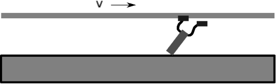
Figure 1: A single motor with the lower end anchored against a glass plate, with its heads binding and unbinding with a microtubule that is being moved at a constant velocity $v$ relative to the plate.

We first consider the problem of a single molecular motor, such as kinesin, with the tail tethered to a substrate such as a glass plate while the heads can freely interact with a long microtubule, as shown in Fig. 1. The microtubule is being moved along a single dimension at uniform velocity $v$ that is parallel to the glass. The heads bind and unbind with the microtubule, applying an average net force $f$, that will depend on $v$. The averaging is being done over time, and we considering the limit where the time interval goes to infinity.

Now consider a collection of $N$ identical motors that all interact with the same microtubule but are sufficiently distant from each other that they can be considered independent. Then the average force acting on the microtubule due to these motors is $Nf$.

The above analysis is easily extended to the case of two separate species of antagonistic motors, labeled $1$ and $2$, with average force versus velocity curves $f_{1}(v)$ and $f_{2}(v)$ respectively, as shown in Fig. 2. If the number of motors of each kind is $N_{1}$ and $N_{2}$, then the time averaged force is $N_{1}f_{1}-N_{2}f_{2}$, where we have adopted a sign convention so that the net force is a difference, rather than a sum. If we choose the ratio $N_{1}/N_{2}=f_{2}(0)/f_{1}(0)$, then this net average force vanishes at $v=0$. This is the “balance point” where there is no net average force acting on the microtubule. The difference between $f_{1}$ and $f_{2}$, $\Delta f(v)$, weighted in this way is shown in Fig. 2.

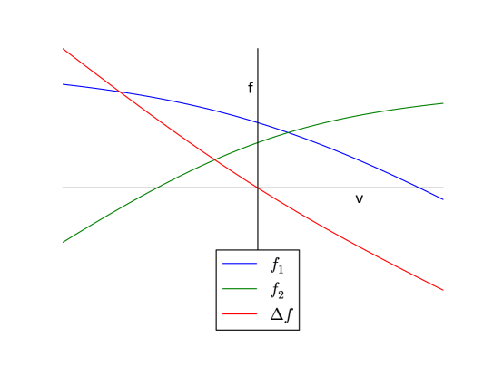
Figure 2: The average force versus velocity curves, $f_{1}$ and $f_{2}$,for two species of motors, $1$ and $2$, that act to antagonize each other. The weighted difference between these two curves, is $\Delta f$, with relative concentrations chosen so that they are at the balance point, so that $\Delta f=0$ for $v=0$.

Note that at small velocities at the balance point, Fig. 2, the net effect of these motors, due to the linear relationship between force and velocity in this regime, is, on average, to give linear drag. This linearity breaks down at high velocities, but, as we will see below, we are interested in the low velocity regime. In this case the net force $f_{n}$ is proportional to $\Delta f$ so that

$$f_{n}=-\gamma v,$$ (1)

where $\gamma$ is the drag coefficient.

Note that if we are not interested in small velocities, there are other phenomena that can take place that can potentially invalidate this analysis. For large enough velocities, the assumption of a fixed force versus velocity curve can sometimes fail ProstJulicherPRL ; GeurinProstMartinJoanny . Some molecular motors at an individual level, are capable of being in two internal states which can be metastable. These two states have different characteristics, and on average, apply their net force in opposite directions. The relative prevalence of the two states depend on the microtubule velocity. If many such motors are simultaneously attached to a microtubule, and allowed to pull it freely, this can lead to the microtubule moving in one direction for a long time and then occassionally, due to the collective fluctuation of all the motors, reversing its direction of motion.

For the problem under discussion here, the two motors are known to be antagonistic and are assumed to be near the balance point, so that the average velocity is very small, and we are therefore justified in taking a time average over very long times, which will then give rise to a single $f$ versus $v$ curve. Therefore we believe that the above behavior is not relevant to our particular case, although it is possible that it could become so, for mixtures of other kinds of motors, and therefore deserves further study.

The above analysis is important for two reasons. First, it relates precisely the force versus velocity curve for assays containing a motor mixture at arbitrary concentration to the behavior of single motor assays. Empirical data on single motor assays can be obtained and then used to understand average properties of these mixed systems. Second, it shows that at the balance point there is only one parameter that need be characterized in order to understand observations; the drag coefficient $\gamma$.

Now that we have understood the behavior of the average force, we shall turn our attention to the effects of spatio-temporal fluctuations on the motion of microtubules. As we shall see, these fluctuations are crucial to understanding the system’s behavior.

II.2 The effect of spatiotemporal fluctuations

We will consider a system at the balance point, where the concentration of the two antagonistic motors has been adjusted as mentioned above, so that the average force on a microtubule is zero. However even at this point, the time averaged force acting on a mictrotubule will depend on its location. This is because the motors are positioned randomly, so that there are fluctuations in the net force. If on average, the number of motors acting on a microtubule is $N$, then we expect this fluctuating time averaged force to have an amplitude that varies proportional to $\sqrt{N}$. This time averaged force will vary slowly as a function of position. If the microtubule is moved only slightly, most of the same motors will still act upon it, meaning that the force will be highly correlated with its original value. The microtubule has to move its entire length before this time averaged force becomes completely independent of its initial value.

Aside from this time averaged force that is position dependent, we can consider a fixed position and ask how the force varies with time. There will be a substantial variation in the force as a function of time due to the random binding and unbinding of motor ends to the microtubule. Because these events are uncorrelated between motors, the amplitude of these fluctuation will also vary proportional to $\sqrt{N}$.

The above considerations imply that there are two parts to the force exerted on the microtubule, a spatially varying component $F(x)$, and a temporal component $n(t)$. For a fixed microtubule, the total force is the sum of these two terms. The statistical properties of $n$ and $F$ are independent of each other because, for a long microtubule, $n$ is the sum of many independent components and therefore its amplitude is independent of position

If we now consider a microtubule that is no longer fixed in position, there is a further force due to the drag, as discussed above.

With these three physical effects included, we are now in a position to model this problem more precisely by characterizing the statistical properties of $n(t)$ and $F(x)$, as we now discuss.

II.3 Model as a Random Walk in Random Environment

Both in a cell and in the experiments, the two motor proteins and microtubules are mixed together in a solution. To model this simply and in one dimension, we imagine a railroad track with motor proteins randomly placed at every tie. This creates a random environment. A rigid microtubule of length $L$, is placed on the tracks, and the motors that lie underneath randomly exert a force on the microtubule. With both species of motors randomly exerting forces on the microtubule in opposing directions, the microtubule undergoes random movement on the track given by

$$\gamma{\dot{x}}=F(x)+n(t),$$ (2)

where $F(x)$ is the random static force, $n(t)$ is the time fluctuating force, and $\gamma$ is the drag coefficient, as discussed above. The left hand side contains $v=\dot{x}$, which is the velocity of the center of mass of the microtubule. Eq. 2 is generally known as a Random Walk in a Random Environment rwre . The difference between this and previous work lies in the correlations in $F(x)$, which as noted above, is correlated over the length of a microtubule.

Below, we will analyze this equation as follows: The random force $n(t)$ gives an effective temperature for this system. By calculating the statistics of the force the motors exert on the microtubule, this temperature can be determined. By calculating the statistics of $F(x)$, we will know how potential correlations behave for length scales much less than $L$. We can thereby estimate how far a microtubule will move, on average, before being stopped by a potential barrier. Using this, we can make estimates about the oscillatory behavior seen in antagonistic gliding assays.

II.4 Determining Forces Exerted on the Microtubule

One railroad tie will by occupied by either a KLP61F or Ncd motor. If we measure the force the motor exerts over a time much longer than that motor’s cycle, we will see an average force

$${\langle}f{\rangle}_{t}=f_{KLP},$$ (3)

for one KLP61F motor, or

$${\langle}f{\rangle}_{t}=f_{NCD},$$ (4)

for one Ncd motor, where $f_{NCD}<0$. Because the motor exerts a peak force for some time and then exerts no force, the average force is given by

$$f_{KLP}=f_{k}p_{k}$$ (5)

for KLP61F, and

$$f_{NCD}=f_{n}p_{n},$$ (6)

for Ncd, where $f_{k}$ and $f_{n}$ are the peak forces exerted by the motors, and $f_{n}<0$. $p_{k}$ and $p_{n}$ are the probabilities of the motors exerting a force on the microtubule. For simplicity, we will set $p_{k}=p_{n}=p$.

The average force exerted by a single motor along the track is determined by the concentrations of the motor species. For a concentration $k$ of KLP61F, the force from one motor site averaged over time and space is given by

$${\langle}{\langle}f{\rangle}_{t}{\rangle}_{x}=kf_{k}p+(1-k)f_{n}p.$$ (7)

For an average net force ${\langle}F{\rangle}=0$, as seen experimentally, the variance of the static force is given by

$${\langle}{\langle}f{\rangle}^{2}_{t}{\rangle}_{x}=k(f_{k}p)^{2}+(1-k)(f_{n}p)^{2}=p^{2}[kf_{k}^{2}+(1-k)f_{n}^{2}].$$ (8)

.

At each motor site, however, the average force is non-zero. Therefore the variance of the time fluctuating force, $n(t)$, is given by

$${\langle}f^{2}{\rangle}-{\langle}f{\rangle}^{2}=kf^{2}_{k}p(1-p)+(1-k)f^{2}_{n}p(1-p)=p(1-p)[kf_{k}^{2}+(1-k)f_{n}^{2}].$$ (9)

II.5 Behavior of the Potential for Distances $\ll L$

Over distances greater than the length of the microtubule, $L$, the potential will look like a random walk, but to determine if the microtubule will fluctuate about a mean position, as seen experimentally, we must look at the potential at scales $\ll L$.

Because ${\langle}F(x){\rangle}=0$, we expect there to be many zeros for $F$ and the dynamics with $n(t)=0$ are such that the microtubule will move downhill in potential to arrive at such points. For finite $n(t)$, the microtubule will still on average move towards lower points in potential, but will fluctuate around local potential minima. Therefore we will look at the fluctuations of a microtubule after it has moved into a position, $x^{*}$, where the $F(x^{*})=0$. This would represent a local minimum of the potential. The question we are addressing here is: are the fluctuations due to $n(t)$ small enough to confine the microtubule to a certain region? In this section, for simplicity we chose our coordinate system so that $x^{*}=0$. Because the force, and therefore the potential, is finite everywhere, and the statistics of the force are translationally invariant, the microtubule cannot be localized to any one region and is expected to eventually move arbitrarily far from an initial point. However we will see that while this is true, the time scale for this happening becomes extremely large, so in practice an experiment will observe confinement of the microtubule to particular region. We will estimate the size of the region that would be explored under normal experimental conditions.

If we move the microtubule a distance, $m$, we will see a difference in the net force exerted on the microtubule. While most of the microtubule is still being moved by the same motors, a length $m$ of it will be moved by new motors. Therefore, the potential will be changed by some amount proportional to a factor of $m$.

The net force exerted along the length of the microtubule is given by

$$F(m)=\sum_{i=\frac{-L}{2}+m}^{\frac{L}{2}+m}\eta_{i},$$ (10)

where $\eta_{i}$ is the force exerted at motor site $i$. Therefore the difference in the net force is

$$F(m)-F(0)=\sum_{i=\frac{-L}{2}+m}^{\frac{L}{2}+m}\eta_{i}-\sum_{i=\frac{-L}{2}}^{\frac{L}{2}}\eta_{i}.$$ (11)

Eq. 11 simplifies because of cancellations on the right hand side, giving

$$F(m)-F(0)=\sum_{j=0}^{m}\phi_{j},$$ (12)

where $\phi$ has been introduced to simplify the right hand side of Eq. 11. Note that all $\phi$’s used below are independent and that ${\langle}\phi^{2}{\rangle}=2{\langle}\eta_{i}^{2}{\rangle}$. As discussed above, we are interested in fluctuations about a potential minimum so that $F(0)=0$.

The potential difference is given by

$$V(x)=-\int^{x}_{0}F(x^{\prime})dx^{\prime}.$$ (13)

Turning Eq. 13 into a Riemann Sum, with segments $\Delta$ equal to the spacing between motors, gives

$$V(m)=-\Delta\sum_{i=0}^{m}f(x_{i})=\Delta\sum_{i=0}^{m}\sum_{j=0}^{j}\phi_{j}=\Delta\sum_{j=0}^{m}j\phi^{\prime}_{j}.$$ (14)

To see how the potential scales with $m$, we look at the average potential difference squared, ${\langle}(V(m)-V(0))^{2}{\rangle}$. To simplify, we will calculate the fluctuations about the minimum, so that $V(0)=0$. Therefore,

$${\langle}(V(m)-V(0))^{2}{\rangle}={\langle}V(m)^{2}{\rangle}=\Delta^{2}\sum_{j=0}^{m}\sum_{i=0}^{m}ij{\langle}\phi^{\prime}_{i}\phi^{\prime}_{j}{\rangle}.$$ (15)

The correlation function ${\langle}\phi^{\prime}_{i}\phi^{\prime}_{j}{\rangle}$ can be determined from the correlation function for individual motors, ${\langle}\eta_{i}\eta_{j}{\rangle}$. Since the motors are regularly spaced, the correlation function is given by,

$${\langle}\eta_{i}\eta_{j}{\rangle}=c\delta_{ij},$$ (16)

because the motors are correlated at distances equal to the motor spacing, and uncorrelated otherwise. The constant c is equal to the variance of the static force, given by Eq. 8. Eq. 16 becomes

$${\langle}\eta_{i}\eta_{j}{\rangle}=p^{2}[kf_{k}^{2}+(1-k)f_{n}^{2}]\delta_{ij}.$$ (17)

Since ${\langle}\phi^{2}{\rangle}={\langle}(\eta_{1}+\eta_{2})^{2}{\rangle}={\langle}\eta^{2}_{1}{\rangle}+{\langle}\eta^{2}_{2}{\rangle}$, the variance of $\phi$ is twice the variance of $\eta$, so that,

$${\langle}\phi_{i}\phi_{j}{\rangle}=2c\delta_{ij}.$$ (18)

Inserting Eq. 18 into Eq. 15 and considering large $m$ yields

$${\langle}V(m)^{2}{\rangle}=2c\Delta^{2}\sum_{i=0}^{m}i^{2}=2c\Delta^{2}\int_{o}^{m}x^{2}dx=\frac{2}{3}c\Delta^{2}m^{3}.$$ (19)

Therefore, the potential fluctuations for distances $m\ll L$ are proportional to $m^{3}$. To calculate how far on average a microtubule will move from a minimum potential, the effective temperature must be determined.

II.6 Determining the Effective Temperature

Determining the effective temperature of the system will tell us the energy of the system and determine how high the potential barriers must be to keep the microtubule trapped in a potential well. We can do this following the standard argument used to show the Fluctuation Dissipation theorem SethnaBookFluctDiss . Determining the diffusion coefficient, $D$, will allow us to make use of the Einstein Relation,

$$D=\frac{k_{B}T}{\gamma}.$$ (20)

The force on the microtubule is given by $f(x,t)=\gamma v$, therefore,

$$\int_{0}^{t}f(t)dt=\gamma(x(t)-x(0)).$$ (21)

Therefore,

$${\langle}\gamma^{2}(x(t)-x(0))^{2}{\rangle}={\langle}(\int_{0}^{t}f(t^{\prime})dt^{\prime})^{2}{\rangle}=\int_{0}^{t}\int_{0}^{t}{\langle}f(t^{\prime})f(t"){\rangle}dtdt^{\prime}.$$ (22)

The correlation function, ${\langle}f(t)f(t^{\prime}){\rangle}$, can be approximated as a delta function, such that

$${\langle}f(t)f(t^{\prime}){\rangle}=2c_{0}\tau_{d}\delta(t-t^{\prime}),$$ (23)

where $c_{0}=p(1-p)[kf_{k}^{2}+(1-k)f_{n}^{2}]$, the variance of the time fluctuating force given by Eq. 9 and $\tau_{d}$ is the decay time of a motor. Substituting Eq. 23 into Eq. 22 gives

$$\int_{0}^{t}\int_{0}^{t}{\langle}f(t^{\prime})f(t"){\rangle}dt^{\prime}dt"=2c_{0}\tau_{d}t.$$ (24)

Setting this equal to the left-hand side of Eq. 22 yields

$$\gamma^{2}{\langle}(\Delta x)^{2}{\rangle}=2c_{0}\tau_{d}t,$$ (25)

with the diffusion coefficient defined as $\frac{1}{2}{\langle}(\Delta x)^{2}{\rangle}$, so that

$$D=\frac{c_{0}\tau_{d}}{\gamma^{2}}.$$ (26)

Using Eq. 26 and the Einstein Relation, Eq. 20 yields an effective temperature

$$k_{B}T=\frac{c_{0}\tau_{d}}{\gamma}.$$ (27)

II.7 Estimating microtubule fluctuation amplitude

To estimate the distance a microtubule moves before encountering a potential barrier of order $k_{B}T$, we set Eq. 19 equal to $(Ak_{B}T)^{2}$, where $A$ is a multiplicative factor, giving

$${\langle}V^{2}{\rangle}=(Ak_{B}T)^{2}=\frac{2}{3}c\Delta^{2}m^{3}.$$ (28)

Solving for $m$ yields,

$$m=[\frac{3(Ak_{B}T)^{2}}{2c\Delta^{2}}]^{\frac{1}{3}}.$$ (29)

Plugging in Eq. 27 yields,

$$m=[\frac{3(A\frac{c_{0}\tau_{d}}{\gamma})^{2}}{2c\Delta^{2}}]^{\frac{1}{3}}=[\frac{3(\frac{A}{\gamma}p(1-p)[kf_{k}^{2}+(1-k)f_{n}^{2}]\tau_{d})^{2}}{2p^{2}[kf_{k}^{2}+(1-k)f_{n}^{2}]\Delta^{2}}]^{\frac{1}{3}}.$$ (30)

If we make the further simplifications that the two motor species exert the same peak force $f_{e}$, the concentrations of the species are equal, and the probability of a motor exerting a force is $\frac{1}{2}$, then Eq. 30 becomes

$$m=[\frac{3(A\frac{f_{e}^{2}\tau_{d}}{4\gamma})^{2}}{\frac{1}{2}f_{e}^{2}\Delta^{2}}]^{\frac{1}{3}}\approx[\frac{(A^{2}f_{e}^{2}\tau_{d}^{2}}{2\gamma^{2}\Delta^{2}}]^{\frac{1}{3}}$$ (31)

According to Ref. Tawada , $\gamma$ can be approximated as $kt$, where $k$ is the effective spring constant of the motor, and t is the characteristic time for the motor to be associated with the microtubule per cycle lisup . Since we approximated $\tau_{d}\approx t$, Eq. 31 becomes

$$m\approx[\frac{Af_{e}}{\sqrt{2}k\Delta}]^{\frac{2}{3}}.$$ (32)

Using $k\approx 1$ pN/nm lisup , $\Delta\approx 50$ nm li , and $f_{e}\approx 10$ pN,

$$m\approx(\frac{A}{2})^{\frac{2}{3}}.$$ (33)

Therefore, to reach a potential barrier of order $10k_{B}T$, the microtubule would have to move $\approx 3$ motor sites, or $0.15$ $\mu$m.

This is in agreement with the fluctuation size of $\approx 0.2\mu m$ measured in motility assays, as in Fig. 5 from Ref. li . Also, it is likely that the potential barrier must be greater than $10k_{B}T$ to contain the microtubule, thereby giving an estimate closer to the experimental result.

In addition, we can determine how the distance the microtubule moves scales with time. According to Kramer’s theory of thermal activation, the time scale $t$ for escaping a potential is proportional to $\exp{t\Delta V/T}$ kramer . Since $\Delta V\sim x^{3/2}$, therefore $x\sim\ln{t^{2/3}}$. Thus, the microtubule can cover a large distance very quickly, but then is trapped in a potential well and restricted to oscillatory motion.

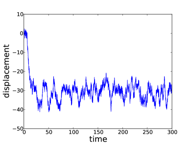
(a) (b)

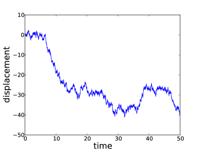
Figure 3: (a) Displacement versus time for a particular realization of random forces. (b) Same plot but expanded for short times. Note that initially it moves until it reaches a position which is more favorable “energetically”.

III Simulations

The analytical work of the last section can be taken further by a numerical implementation of the model described by Eq. 2. We use units of length so that the distance between adjacent motors is unity.

We consider a force produced by a motor at the $ith$ site, $f_{i}$, drawn from a standard normal distribution. The net force acting on a microtubule, $F(j)$, is the sum over $L$ adjacent sites of these random forces, as in Eq. 10. We then linearly interpolate for non-integral values of $x$ to obtain the force at an arbitrary position which gives us the complete force for any value of $x$. We choose $n(t)$ from a Gaussian distribution with standard deviation $C$, to describe the system at a temperature $T$. We solve Eq. 2 by a simple Euler discretization with a time step $dt=0.01$. The noise amplitude is related to the temperature by $C=\sqrt{2T/dt}$.

Fig. 3 shows a single run for one a random realization of random forces. The displacement starting from $x=0$ is shown as a function of time in (a). Fig. 3(b) shows the same data rescaled to reveal the behavior of the initial transient. Note that the microtubule moves approximately 35 units before finding a deep potential minimum. Figure 4 displays the corresponding histogram of microtubule position. The initial transient behavior was not included. The non-Gaussian shape is due to the underlying roughness of the force $F(x)$ and its corresponding potential. For extremely long times, this histogram will change because the microtubule will eventually be able to overcome enormous energy barriers. However the corresponding times for these are exponentially large as discussed in the previous section. Under experimentally reasonable time scales, we expect this kind of histogram to be obtained.

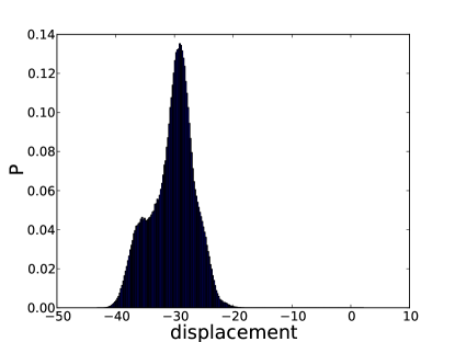
Figure 4: Histogram of positions. The initial transient was not included.

We now probe the behavior of the initial transients, noted above. We ran this simulation $300$ times each with randomly generated forces. Then we computed the initial displacement for each realization by taking the difference between the steady state average position and the initial position. A histogram of these differences is shown in Fig. 5. As is apparent, the displacement in a transient is typically about $100$, or the length of the microtubule.

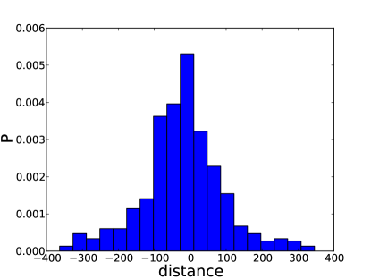
Figure 5: A histogram of the displacement due to the initial transients. The simulation was run $300$ times and the initial displacements were all computed. The initial displacement was obtained by taking the difference between the steady state average position and the initial position of the microtubule.

IV Model application to interpolar microtubules during metaphase

We have seen that the effect of antagonistic motors is indeed to lead to a quasi-steady state behavior for gliding assays where microtubules fluctuate in a localized region. However there is a sizeable initial transient displacement that appears to be of order the length of the microtubule before it becomes localized.

The reason for this relatively large initial transient can be understood from the statistics of random walks. The time averaged net force $F$, is the sum of the forces of the individual motors, Eq. 10, and the displacement from that point will follow random walk statistics for lengths smaller than the length of the microtubule $L$ as seen from Eq. 11. Typically $F$ will have a magnitude that scales as $\sqrt{L}$. If we are interested in how far a microtubule must travel before $F=0$, then this must be a distance that is proportional to $L$, because this will typically give rise to a change in force that is also proportional to $\sqrt{L}$.

Figure 6: Two anti-parallel microtubules interacting via two types of antagonistic motors. The motors interact in the region of overlap.

Now consider the slightly different situation of competitive motors interacting on antiparallel microtubules, interacting with each other as shown in Fig. 6. The motors will only operate in the region where the microtubules overlap, which in the figure is over a distance of length $x$, corresponding to $n=x/\Delta$ motors. Eqn. 10 is modified to be

$$F(m)=\sum_{i=0}^{m}\eta_{i},$$ (34)

where $\eta_{i}=f_{1,i}+f_{2,i}$ is the sum of the effects motors walking on both microtubules. This form is different from the gliding assay case, because now the number of motors included in the sum depends on the overlap distance $x$. However $F(m)$ is still of the form of a random walk. Therefore the total force is not expected to vanish except possibly at a finite number of random values of $x$. The microtubules are therefore expected to have transients that are also large, but different than the case of the gliding assays.

Because the force has the form of a random walk, and we are interested in where it passes through zero, this problem is equivalent to the first passage time problem of a random walk where here the position of the random walk is in force space and time for the random walks becomes the distance of overlap $x$. In the case where the microtubule move to increasing $x$, this would be equivalent to a random walk that starts off some distance from zero and asking how long it will take to cross zero. In this case, if the distance of overlap starts out as $x_{0}$, it will experience a random force $F_{0}$, which is the sum of separate motor forces, see 34. In the absence of external forces, the microtubules will slide until they reach an overlap $x^{*}$ such that $F(x^{*})=0$. As in the gliding assay case, this will be a distance of order $x_{0}$.

On the other hand, if the microtubule moves in a direction of decreasing $x$, then the statistics of $F(m)$ will be that of a random walk that starts out with $F(0)=0$. The probability of a random walk of length $m$ starting at the origin but never passing through zero can be obtained  chandrasekhar . For example, if the motor spacing $\Delta=50nm$ and the overlap $x=1\mu m$, then we are asking for the probability that a random walk of length $20$ never passes through its starting position. In that case that probability is about $0.18$. This means that many overlapping microtubules will be pushed away from each other so that they no longer overlap. Many others will increase from an overlap of $1\mu m$ to greater than $2\mu m$.

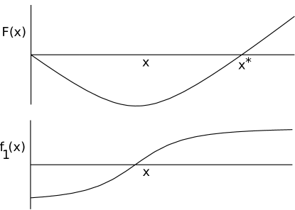
Figure 7:

Therefore this model of motor association during prometaphase, does a somewhat imperfect job of maintaining spindle length. One simple way to improve its efficacy is to have a gradient in motor concentrations. In this case in Eq. 34, instead of the forces $f_{1}$ and $f_{2}$ being random variables with a mean zero, we say that the local motor concentrations are not at the balance point so that there is a net time averaged force that varies deterministically with position. Let us further assume that the concentration profile is the same for both microtubules. Then the corresponding force densities $f_{1}(x)$ and $f_{2}(x)$, will give equal contributions to the net force that the microtubules exert on each other.

$$F(x)=2\int_{0}^{x}f_{1}(x^{\prime})dx^{\prime}.$$ (35)

Fig. 7 displays a force density profile that has the right properties. $f_{1}(x)$ starts of negative, close to $x=0$, meaning that near the tip of the microtubules, the motors have the net effect of pulling each other closer together. At some point the sign of $f_{1}(x)$ changes and motors in that region predominantly pull the microtubules apart. The net force due to all the motors as a function of overlap, $F(x)$ is obtained by integrating $f_{1}(x)$. The equilibrium overlap $x^{*}$ is when $F(x^{*})=0$. By adjusting the profile of motor concentrations, $x^{*}$ can be shifted.

IV.1 Strength of concentration imbalance

One caveat that should be mentioned is that if the motor concentration gradients are too weak, then the microtubules will become stuck due to the randomly fluctuating force. Without a strong enough bias due to motor concentration variation, the extremely jagged random environment will prevent microtubules from sliding to the equilibrium point $x^{*}$. We now consider the minimum size of this concentration variation necessary to overcome the random static forces.

The force in Fig. 7 is linear around the equilibrium point $x^{*}$, and is of the form of Hooke’s law: $F=-\kappa x$, where $x$ is measured relative to $x^{*}$. The maximum value that $\kappa$ can take can be determined by the extreme case where the force on the microtubule changes from $0$ to $f_{e}$ within one motor spacing $\Delta$. If this change occurs over a width of $n$ motors instead, we can write $\kappa=f_{e}/(n\Delta)$. We wish to determine the maximum value of $n$ that is consistent with the microtubules being able to slide relative to each other. The potential corresponding to Hooke’s law is $U=\kappa x^{2}/2$. Compared with the statistics of the random potential, Eq. 28, where $V\propto x^{3/2}$, we see that for small enough $x$, the random force dominates, but when $x$ becomes sufficiently large, Hooke’s law prevails. If the crossover occurs at too large a value of $x$, then the system will become trapped in some local random minimum and not be able to move closer to $x^{*}$. To determine this crossover, we equate the standard deviation of the fluctuation in the random potential, given by Eq. 28, with the Hookean potential. In terms of $m=x/\Delta$, we obtain

$$n^{2}=\frac{3}{8}\frac{f_{e}^{2}m}{c},$$ (36)

where the force variance $c$ is given in Eq. 17. To estimate the value of $n$, we take $p=1/2$, and $f_{k}=f_{n}=f_{e}$. This gives $n^{2}=(3/2)m$. Experimentally in a gliding assay, it was found that the fluctuations in $m$ where approximately 4. This means that we expect that $n$ should be in the range 2 to 3, in order for the microtubules to slide within the experimental time scale.

This small value of $n$ is consistent with the fact that at the balance point, the fluctuations in position of a microtubule in a gliding assay are small. The spacing between motors, in these assays, is presumably not identical to interpolar microtubules in the spindle but they are believed to be plausibly similar li ; BrustMascher .

V Conclusion

By means of a fairly general analysis, making few assumptions, we have seen that the motion of microtubules in an antagonistic motility assay near the balance point, is well described by a random walk in a random environment,rwre but with large correlations in the static random force. The connection does not depend on a detailed model of the motors. The force velocity curves of the motors near the stall point, $v=0$, only come into play to give a drag coefficient for the microtubule. The results found are in reasonable agreement with the fluctuations observed in microtubule positions seen in experiments li . However the model also predicts that the microtubule will slide of order their own distance before getting badly trapped.

There is substantial similarity between these gliding assay experiments and models for what occurs in vivo during prometaphase, with KLP61F and Ncd motors antagonizing each other in mitotic spindles li ; civelekoglu . However we point out that although their model correcly predicts that these motors will act to inhibit variations in spindle length, they also do so imperfectly. Antiparallel interpolar microtubules will have initial transients where they slide of order their own length, or sometimes completely disassociate. It appears that such variations are within the error bars of experimental observation however. But, to circumvent these fluctuations, it is possible that the cell sets up a gradient of motors during prometaphase, thereby restricting the mitotic spindle to oscillatory movements in a potential well. Further observations of the densities of motors in vivo could lend a great deal to further understanding of this situation.

VI Acknowledgments

This material is based upon work supported by the National Science Foundation under Grant CCLI DUE-0942207.

References

- (1) Heck, M.M., Pereira, A., Pesavento, P., Yannoni, Y., Spradling, A.C., and Goldstein, L.S. (1993). The kinesin-like protein KLP61F is essential for mitosis in Drosophila. J. Cell Biol. 123, 665-679.
- (2) Sharp, D.J., Yu, K.R., Sisson, J.C., Sullivan, W., and Scholey, J.M. (1999). Antagonistic microtubule-sliding motors position mitotic centrosomes in Drosophila early embryos. Nat. Cell Biol. , 51Ð54.
- (3) Brust-Mascher, I., and Scholey, J.M. (2002). Microtubule flux and sliding in mitotic spindles of Drosophila embryos. Mol. Biol. Cell 13, 3967Ð3975.
- (4) Tao, Li, Jonathan M. Scholey, et al. “A Homotetrameric Kinesin-5, KLP61F, Bundles Microtubules and Antagonizes Ncd in Motility Assays.” Current Biology. 16 (2006): 2293-2302.
- (5) Gul Civelekoglu-Scholey, Li Tao, Ingrid Brust-Mascher, Roy Wollman, and Jonathan M. Scholey, Prometaphase spindle maintenance by an antagonistic motor-dependent force balance made robust by a disassembling lamin-B envelope, J. Cell Biol. 188 49–68 (2010).
- (6) F. Jülicher, J. Prost, “Spontaneous oscillations of collective molecular motors” Phys Rev Lett, 78 4510–4513 (1997).
- (7) T. Guérin, J. Prost, P. Martin, J F Joanny, “Coordination and collective properties of molecular motors: theory” Curr. Opinion Cell Bio. 22, 14–20 (2010).
- (8) Marinari, E, G Parisi, D Ruelle, and P Windey. “Random Walk in a Random Environment and 1/f Noise.” Physical Review. 50.17 (1983).
- (9) J.P. Sethna “Statistical Mechanics Entropy, Order Parameters and Complexity” Page 227. Oxford University Press (2006).
- (10) Tawada, K., and Sekimoto, K. (1991). Protein friction exerted by motor enzymes through a weak-binding interaction. J. Theor. Biol. 150, 193Ð200.
- (11) Tao, Li, Jonathan M. Scholey, et al. “Supplemental Data to A Homotetrameric Kinesin-5, KLP61F, Bundles Microtubules and Antagonizes Ncd in Motility Assays.” Current Biology. 16 (2006): 2293-2302.
- (12) Kramer, H.A. (1940). Brownian motion in a field of force and the diffusion model of chemical reaction. Physica. 7.4, 284-304.
- (13) (1948) Stochastics Problems in Physics and Astronomy Rev. Mod. Phys. 15 1-85
- (14) Brust-Mascher, I., Civelekoglu-Scholey, G., Kwon, M., Mogilner, A., and Scholey, J.M. (2004). Model for anaphase B: Role of three mitotic motors in a switch from poleward flux to spindle elongation. Proc. Natl. Acad. Sci. USA 101, 15938–15943.