Quantum Gibbs distribution from dynamical thermalization in classical nonlinear lattices

Abstract

We study numerically time evolution in classical lattices with weak or moderate nonlinearity which leads to interactions between linear modes. Our results show that in a certain strength range a moderate nonlinearity generates a dynamical thermalization process which drives the system to the quantum Gibbs distribution of probabilities, or average oscillation amplitudes. The effective dynamical temperature of the lattice varies from large positive to large negative values depending on energy of initially excited modes. This quantum Gibbs distribution is drastically different from usually expected energy equipartition over linear modes corresponding to a regime of classical thermalization. Possible experimental observations of this dynamical thermalization are discussed for cold atoms in optical lattices, nonlinear photonic lattices and optical fiber arrays.

Dated: July 22, 2013

1 Introduction

The problem of thermal distribution for photons led to the invention of the Planck constant and Planck law [1]. Further development of quantum mechanics generalized the Gibbs thermal distribution [2] to the quantum case leading to the quantum Gibbs distribution in a quantum system with discrete energy levels (see e.g. [3, 4]). Thus the problem of thermalization was always fascinating the scientists starting from the famous dispute between Boltzmann and Loschmidt on time reversibility and statistical description (see e.g. [4]).

The thermalization in a given system is based on the ergodicity of motion which can be produced by noise from a heat bath or by internal dynamical chaos. The mathematical and physical foundations of dynamical chaos are now well established and are described in [5, 6, 7, 8]. The first numerical investigations of onset of ergodicity and dynamical thermalization in a nonlinear lattice of coupled oscillators had been performed for the Fermi-Pasta-Ulam problem [9, 10, 11, 12] with an expectation to find energy equipartition over linear oscillator modes. Surprisingly, for a typical set of parameters the equipartition was absent, even if in certain cases signs of non-periodic behaviour were visible. The absence of ergodicity stimulated a great interest to the Fermi-Pasta-Ulam problem even if later it became clear that this model is rather close to the integrable Toda lattice and, hence, it does not belong to a class of generic models (see discussions in [8, 11, 12]).

Another approach to investigation of onset of ergodicity over linear oscillator modes in nonlinear lattices had been proposed in [13] by analyzing the effects of nonlinearity on the Anderson localization [14] in systems with disorder or systems of quantum chaos. It was found that below a certain critical nonlinearity a spreading over modes is suppressed or is exponentially slow while at moderate nonlinearity a sub-diffusive spreading continues up to times being by millions time larger than a typical time scale of oscillations. This result has been confirmed and significantly extended by further investigations [15, 16, 17, 18, 19, 20, 21, 22, 23, 24, 25, 26], however the full understanding of the problem is still lacking. Thus the results [24] indicate that at large times the spearing continues along certain chaotic but non-ergodic layers. The mathematical studies [27, 28, 29] demonstrate all the complexity of this problem where pure-point spectrum of linear system generates intricate resonances induced by nonlinearity. The interest to the problem is also supported by experiments with disordered nonlinear photonic lattices [30, 31] and Bose-Einstein condensates of cold atoms placed in a disordered optical lattice [32].

Recently it was argued that in the discrete Anderson nonlinear Schödinger equation (DANSE) a process of dynamical thermalization takes place leading to a statistical equilibrium in a finite disordered lattice at a moderate nonlinearity [33]. It was shown numerically that the Gibbs energy distribution takes place over linear eigenmodes. This work generated a certain interest to the process of dynamical thermalization in weakly nonlinear lattices [34]. It was also pointed out that such a thermalization is necessary for emergence of Kolmogorov turbulence in finite size systems [35].

Here we extend the studies of dynamical thermalization in disordered lattices with weak or moderate nonlinearity. We especially stress the situation when the energies of linear modes grow linearly with index of linear modes corresponding to a static Stark field or finite density of levels in a unit energy (frequency) interval. Such a case is typical for the Kolmogorov (or weak wave) turbulence in finite systems [36, 37]. As an example of such a system we can name the nonlinear Schrödinger equation in the Sinai billiard (or any other chaotic billiard) as discussed in [35]. It is also important to note that the DANSE with a static field is also characterized by a subdiffusive spreading [38].

In this work we extend the research line of dynamical thermalization in nonlinear disordered lattices investigating a large number of models. Surprisingly, our results show that in lattices with weak or moderate nonlinearity there is emergence of a quantum Gibbs distribution over energies of linear eigenmodes. In some sense the weak nonlinearity acts as a dynamical thermostat creating a quantum Gibbs distribution. We discuss the conditions under which such a quantum Gibbs replaces a usually expected energy equipartition over linear modes predicted by the classical thermalization theory [3, 4, 5, 6, 7, 8].

The paper is constructed as follows: in Section 2 we describe all nonlinear lattice models investigated in this work, in Section 3 we introduce the quantum Gibbs anzats, results for 1d models $M1,M2$ and 2d models $M3,M4$ are presented in Sections 4 and 5, the results for the Klein-Gordon lattice are given in Section 6, the discussion of the results is presented in Section 7.

2 Description of nonlinear lattice models

To investigate the phenomenon of emergence of a quantum Gibbs distribution we study several models of linear lattices with disorder and additional weak or moderate nonlinear terms. These models represent one-dimensional (1d) and two-dimensional lattices (2d) which in absence of nonlinearity can be reduced to the Anderson model of non-interacting electrons (see e.g. [39]) on a disordered lattice in 1d and 2d respectively.

The main DANSE model [16] is described by the equation:

$$i\hbar{{\partial{\psi}_{n}}\over{\partial{t}}}=E_{n}{\psi}_{n}+{\beta}{\mid{\psi_{n}}\mid}^{2}\psi_{n}+V({\psi_{n+1}}+{\psi_{n-1})}\;.$$ (1)

In the following we use dimensionless units with $\hbar=V=1$, the Boltzmann constant is taken to be unity so that we have all dimensionless variables. In total we consider the lattice with $N$ sites and periodic boundary conditions. For $E_{n}=0$ and long wave limit the system is reduced to the nonlinear Schrödinger equation which is also known in the field of cold atoms as the Gross-Pitaevskii equation [40]. At $\beta=0$ and random values of $E_{n}$ distributed in the interval $-W/2\leq E_{n}\leq W/2$ the system (1) represents the 1d Anderson model with the localization length $\ell\approx 96/W^{2}$ [39]. For this distribution of $E_{n}$ and nonzero $\beta$ the equation (1), named as the DANSE model, was discussed and investigated in [13, 15, 16, 17, 18] and other papers.

The Hamiltonian of DANSE has the form

$$H=\sum_{n}E_{n}|\psi_{n}|^{2}+\psi_{n-1}\psi_{n}^{*}+\psi_{n-1}^{*}\psi_{n}+\frac{\beta}{2}|\psi_{n}|^{4}\;,$$ (2)

with $\psi_{n}$ and $\psi_{n}^{*}$ being the conjugated variables. The energy and the probability norm $\sum_{n}|\psi_{n}|^{2}=1$ are exact integrals of motion. The Hamiltonian (2) can be rewritten in the basis of linear eigenmodes $\varphi_{nm}$ related to $\psi_{n}=\sum C_{m}\varphi_{nm}$. In the eigenmode representation the Hamiltonian is

$$H=\sum_{m=1}^{N}\epsilon_{m}|C_{m}|^{2}+\beta\sum_{m_{1}m_{2}m_{3}m}V_{m_{1}m_{2}m_{3}m}C_{m_{1}}C_{m_{2}}C^{*}_{m_{3}}C^{*}_{m},$$ (3)

with $\sum_{m}|C_{m}|^{2}=1$, and $V_{{m}{m^{\prime}}{m_{1}}{m_{1}^{\prime}}}\sim\ell^{-3/2}$ being the transition matrix elements [13] (the dependence on $\ell$ is given assuming random matrix estimate for eigenstates overlap). From this representation it is especially clear that the spreading takes place only due to the nonlinear $\beta$ coupling.

In 1d we consider the extensions of the DANSE model given by the following replacements in Eq. (1):

$$E_{n}\rightarrow E_{n}+f|n-n_{0}|\;,\;(M1)\;.$$ (4)

Here $E_{n}$ have the same random distribution as in DANSE, $n_{0}=(N+1)/2$ marks the center of the lattice and the periodic conditions link sites $N$ and $1$. This is the model $M1$ with the static Stark field $f$ which models the constant density of states in energy as it is the case in the quantum Sinai billiard [35].

We also study the model $M2$ which is obtained from $M1$ by the following replacement of the nonlinear term:

$$\beta\rightarrow\beta|n-n_{0}|\;,\;(M2)\;.$$ (5)

In this model $M2$ the nonlinear term grows with the level number that often happens for nonlinear wave interactions in wave turbulence (see e.g. [36, 37, 41]).

We also analyze the 2d DANSE lattice studied in [19]:

$$i{{\partial{\psi}_{n_{x}n_{y}}}\over{\partial{t}}}=E_{n_{x}n_{y}}{\psi}_{n_{x}n_{y}}+{\beta}{\mid{\psi_{n_{x}n_{y}}}\mid}^{2}\psi_{n_{x}n_{y}}$$

$$+({\psi_{n_{x}+1n_{y}}}+{\psi_{n_{x}-1n_{y}}}+{\psi_{n_{x}n_{y}+1}}+{\psi_{n_{x}n_{y}-1}})\;.$$ (6)

Periodic boundary conditions are used for $N\times N$ square lattice with $-N/2\leq n_{x},n_{y}\leq N/2$. However, here we use the extended version of this model assuming that

$$E_{n_{x}n_{y}}=\delta E_{n_{x}n_{y}}+f(n_{x}^{2}+n_{y}^{2})\;,\;-W/2\leq\delta E_{n_{x}n_{y}}\leq W/2\;,\;(M3)\;.$$ (7)

This is the model M3 with random values of energies $\delta E_{n_{x}n_{y}}$ in a given interval.

In addition we study the model $M4$ obtained from the model $M3$ by the replacement

$$\beta\rightarrow\beta(n_{x}^{2}+n_{y}^{2})\;,\;(M4)\;.$$ (8)

This is the 2d analog of model $M2$.

Since the term $(n_{x}^{2}+n_{y}^{2})$ grows linearly with index $k=|n_{x}|+|n_{y}|$ we can consider the model $M3$ as the model for the nonlinear Schrödinger equation in the Sinai billiard (see Eq.(6) at $F=0$ in [35]). Indeed, in a Sinai billiard the energy levels are randomly and homogeneously distributed over the energy axis, as it is the case in model $M3$ at $f>0$, and also the nonlinear term has a similar form coupling the linear modes. The advantage of $M3$ model is that it is significantly easier for numerical simulations compared to the case of Sinai billiard. The model $M4$ has a stronger nonlinear interactions at high wave vectors that is typical for the weak wave turbulence [36, 37].

We note that 2d models $M3$, $M4$ also can be written in the form (3) with more complex matrix elements induced by the nonlinear coupling on 2d lattice.

The above models $M1,M2,M3,M4$ have two integrals of motion being energy and the wavefunction norm. The latter is generally absent in nonlinear lattices. For this reason we consider the Klein-Gordon lattice (KG model) described by the Hamiltonian:

$$H=\sum_{l}[(p^{2}_{l}+{\tilde{\epsilon}_{l}}u_{l}^{2})/2+\beta u_{l}^{2}/4+(u_{l+1}-u_{l})^{2}/(2W)],$$ (9)

where $\tilde{\epsilon}_{l}$ are taken as random in the interval $[1/2,3/2]$ (see e.g. [18]). This KG model was studied in [18] and it was shown that it has the same type of subdiffusive spreading as DANSE. We keep the same notations as in [18] (see Eq.(6) there) but we introduce the nonlinear coefficient $\beta$ (it is taken at $\beta=1$ in [18]) and we add a static field $f$ replacing $\tilde{\epsilon}_{l}\rightarrow\tilde{\epsilon}_{l}+f|l-l_{0}|$ keeping the random distribution in the same interval (in [18] $f=0$). We use $l_{0}=(N+1)/2$ and periodic conditions linking sites $l=1$ and $N$. As shown in [18], the linear part of the Hamiltonian at $f=0,\beta=1$ can be reduced to the 1d Anderson model.

The time evolution of models $M1,M2,M3,M4$ was integrated numerically using the symplectic integration scheme as described in [19]; the KG model was integrated by $SABA_{2}C$ method described in [18]. The time average is done over the time interval $\delta t$ in a vicinity of time $t$. The integration time step was fixed at $\delta t=0.05$ for all models but we checked that its decrease by a factor $10$ did not affect the results of numerical simulations.

3 Quantum Gibbs anzats

For the DANSE and $M1,M2,M3,M4$ models we make a quantum Gibbs conjecture that the nonlinear terms act like some kind of dynamical thermostat which creates the quantum Gibbs distribution over quantum states with linear mode eigenenergies $\epsilon_{m}$. Then according to the standard relations of statistical mechanics [3, 4] we find the probabilities $\rho_{m}=|C_{m}|^{2}$ and the statistical sum $Z$ of the system:

$$\rho_{m}=Z^{-1}\exp(-\epsilon_{m}/T)\;,\;Z=\sum_{m}\exp(-\epsilon_{m}/T)\;.$$ (10)

Here, $T$ is a certain temperature of our isolated system which depends on the initial energy given to the system. As usually for any quantum system with energy levels $\epsilon_{m}$ we have the total probability $\sum_{m}\rho_{m}=1$ and total energy $E=\sum\rho_{m}\epsilon_{m}$ (here we neglect a small nonlinear term correction to energy). The norm conservation can also taken into account using the standard approach of statistical mechanics with the chemical potential and conservation of number of particles (or norm) [3, 4] that is equivalent to the normalization used in (10). We note that possibilities of thermalization has been discussed in nonlinear chains starting from the FPU problem [9, 10, 11, 12] and continuing even for nonlinear breathers [42, 43, 44]. However, here we consider the case of weak or moderate nonlinearity when the nonlinear terms are relatively small comparing to linear quadratic terms. In this case the classical system is expected to reach energy equipartition over linear modes [3, 4, 45, 46].

The entropy of the system can be expressed via the average probability $\rho_{m}$ on level $m$ via the usual formula:

$$S=-\sum_{m}\rho_{m}\ln\rho_{m}\;,\qquad\rho_{m}=\overline{|C_{m}|^{2}}\;,$$ (11)

where overline means time averaging.

• 

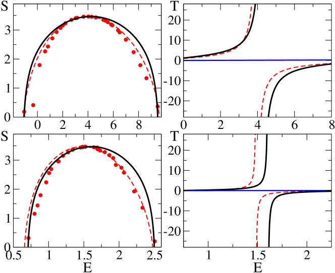
Figure 1: Top panels: (left) the dependence of entropy $S$ on energy $E$ from the quantum Gibbs anzats (10) with $\epsilon_{m}$ taken from a given disorder realisation in $M1$ (red dashed curve), the numerical data from time evolution of $M1$ are shown by red points at $t=10^{7}$ with $\delta t=10^{6}$; the full black curve shows the dependence from the Gibbs anzats (10) for equidistant levels $\epsilon_{m}={\tilde{f}}m/2$ with ${\tilde{f}}=2(\epsilon_{max}-\epsilon_{min})/N\approx 1.32f$ (where $\epsilon_{max}=9.51$ and $\epsilon_{min}=-1.05$) for a given disorder realization (see text); here $f=0.5$, $\beta=2$, $W=2$, $N=32$; (right) temperature dependence $T(E)$ from the quantum Gibbs anzats (10) with the same cases as in left panel, blue curve shows the classical equipartition dependence $T=E/N$, numerical data are not shown here. Bottom panels: same as in the top panels but for the $KG$ model at $f=0.125$, $\beta=1$, $W=2$, $N=32$, $\epsilon_{max}=2.51$ and $\epsilon_{min}=0.71$, numerical evolution is followed up to $t=10^{8}$ with $\delta t=10^{6}$.

The entropy $S$, energy $E$ and temperature $T$ are related to each other via the standard thermodynamics expressions [3]:

$$E=T^{2}\partial\ln Z/\partial T\;,\;\;S=E/T+\ln Z\;,\;\;\partial S/\partial E=1/T\;.$$ (12)

This value of entropy yields the maximal possible equipartition for a given initial energy. In an implicit way, a value of energy $E$ determines the temperature $T$ of the system and its entropy, or by varying temperature $T$ in the range $(-\infty,+\infty)$ we obtain the variation $E(T)$, $S(T)$ and implicitly the curve $S(E)$. The advantage of variables $E,S$ is based on the fact that they both are extensive variables [3, 4] and thus they are self averaging and hence in numerical simulations they have significantly smaller fluctuations comparing e.g. to temperature $T$. It is important to note that the above quantum Gibbs relations can be also obtained from the condition that the entropy $S$ takes the maximal value at variation of probabilities $\rho_{m}$.

In fact the quantum Gibbs anzats was introduced in [33] for the DANSE and it was shown that it works at moderate nonlinearity $\beta$ and not very strong disorder $W$ (see also discussions in [44]). However, in [33] the striking paradox of quantum Gibbs anzats was not pointed out directly. Indeed, the nonlinear classical lattice is expected to have energy equipartition over linear modes that is in a drastic contrast with the quantum Gibbs distribution described above.

The examples of dependence $S(E)$ and $T(E)$ produced by the quantum Gibbs anzats for the models $M1$ and $KG$ are shown in Fig. 1. We use one disorder realisation with eigenvalues $\epsilon_{m}$ for $M1$ and $\epsilon_{m}=\omega_{m}^{2}/2$ for $KG$ (more details on KG model are given in Section 6). To compare the numerical data obtained from time evolution with the Gibbs anzats we use the exact eigenenergies $\epsilon_{m}$ obtained from exact matrix diagonalization of the linear problem at a given disorder realisation. Examples of dependence of $\epsilon_{m}$ on index $m$ are shown in Fig. 2 for the model $M1$. We also can use the average dependence $\epsilon_{m}\approx{\tilde{f}}m/2$ ($1\leq m\leq N$) with ${\tilde{f}}=2(\epsilon_{max}-\epsilon_{min})/N$ which in an approximate manner takes into account the disorder fluctuations with the maximal $\epsilon_{max}$ and minimal values of $\epsilon_{min}$ linear eigenenergies. This approach of an effective average density ${\tilde{f}}$ gives a good description of numerical data (see Fig. 1). It gives a slight shift of the maximum of $S(E)$ curve which is more sensitive to a disorder and is not of principal importance. We return to the discussion of $KG$ model in Section 6.

• 

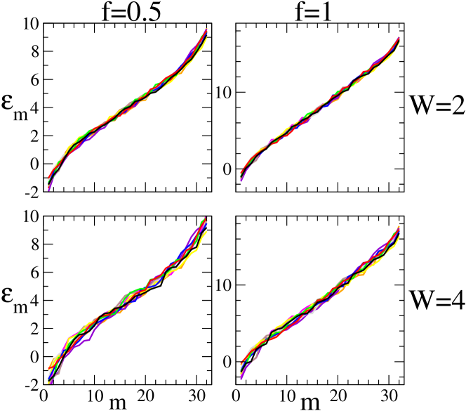
Figure 2: Dependence of eigenenenergies $\epsilon_{m}$ of linear eigenmodes on mode index $m$ in $M1$ for parameters of Fig. 1 at $f=0.5;1$ (ten disorder realisations are shown by different color curves).

In contrast to the quantum Gibbs distribution the classical thermodynamics implies the energy equipartition over all modes [3, 4] that gives:

$$T=(E-E_{min})/N\;,\;\;S=N\ln(E-E_{min})+C_{0}\;,$$ (13)

where $E_{min}$ is a certain minimal energy of the system and $C_{0}$ is a numerical constant. The results of Fig. 1 show the drastic difference between the predictions of quantum and classical thermodynamics.

The dependence $S(E)$ has one maximum and according to the standard thermodynamics relations (12) the system has a negative temperature $T<0$ at the right branch of $S(E)$ curve. It is known that such situations can appear in quantum systems with energies located in a finite band width [3, 4]. We note that recent experiments with cold atoms in optical lattices [47] allowed to realise finite quantum systems at negative temperatures.

We should stress that the quantum Gibbs distribution we find has close similarities with the thermal quantum distribution in real quantum systems however it appears as a result of dynamical thermalization in weakly nonlinear classical coupled oscillators without any second quantization. This Gibbs distribution results from dynamical thermalization and entropy maximization over linear modes without real quantum Plank constant entering in the game. In this respect our physical interpretation is very different from the one developed in [48] where the authors discussed appearance of the real quantum Planck constant in the thermal equilibrium of classical nonlinear lattices. In our consideration we have an effective Planck constant which may be effectively introduced in a system of weakly coupled nonlinear oscillators (e.g. as a typical frequency difference between frequencies for DANSE or KG models).

Below we present the numerical results on the detailed verification of the quantum Gibbs anzats for various lattice models.

4 Results for 1d lattice models

The dependencies $S(E)$ for 1d lattice models $M1,M2$ are shown in Figs. 3,4.

For $M1$ we see that at $\beta=2$ the quantum Gibbs works well at $f=0.5$ and $W=2$. At fixed $W$ an increase of $f$ leads to appearance of a significant number of non-thermalized modes at $f=2$. Indeed, at large $f$ the average distance between linear modes is growing $\Delta\omega\approx f$ and a nonlinear frequency broadening $\delta\omega$ becomes to be too small so that the nonlinear coupling between linear modes starts to be perturbative and the integrability sets in for larger and larger number of initially excited modes. A similar situation for $3$ oscillators with a nonlinear coupling had been discussed in [49]. An increase of disorder from $W=2$ up to $W=4$ reduce the localization length $\ell$ and the number of coupling terms between linear modes drops. This leads to a larger number of non-thermalized modes.

• 

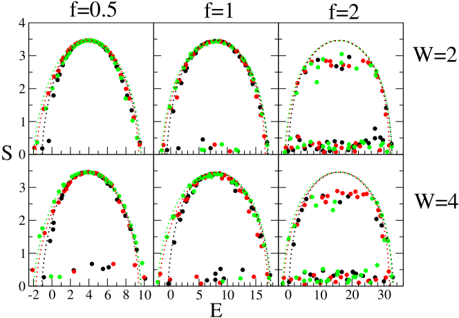
Figure 3: Dependence of entropy $S$ on energy $E$ for initial excited eigenmodes of the linear problem in 1d model $M1$. The value of entropy $S$ is obtained by time averaging over a time interval $\delta t=10^{6}$, at time $t=10^{7}$, the energy $E$ is taken as the total energy of the lattice when the linear eigenmode $m$ is excited at time $t=0$ ($1\leq m\leq N$). The numerical data are shown by points for 3 disorder realisations (black, green, red), the corresponding theoretical quantum Gibbs distributions, with the exact linear eigeneinergies $\epsilon_{m}$ for a give disorder realisation, are shown by dotted curves of the same color. The values of disorder strength $W$ and Stark field $f$ are given in the figure; here $\beta=2$, $N=32$.

For the model $M2$ in Fig. 4 we take a relatively small value of nonlinearity $\beta=0.2$. Thus at $m<m_{c}\approx N/3$ we have a local effective $\beta_{eff}\approx\beta|m-n_{0}|<1$, thus the dynamics remains mainly integrable and the dynamical thermalization is absent for low energy modes. However, at $m>m_{c}\approx N/3$ we have the onset of dynamical thermalization and the Gibbs law works for high energy modes. With the increase of time we see the increase of number of thermalized modes at $m>m_{c}$.

• 

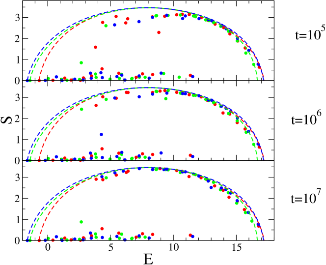
Figure 4: Dependence of entropy $S$ on energy $E$ at three moments of time $t$ for three disorder realisations in 1d model $M2$ at $f=1$, $W=2$, $\beta=0.2$, $N=32$; the averaging is done in the time interval $\delta t=t/10$. Points show the numerical data for three disorder realisations (three colors), dotted curves show the corresponding theoretical Gibbs distributions.

5 Results for 2d lattice models

The results for 2d lattice models $M3,M4$ are presented in Figs. 5, 6. We note that the model $M3$ can be also viewed as a model for a nonlinear interaction of laser modes in optical fibers which $z$-propagation along the fiber is analogous to the time evolution in our model. At present the nonlinear dynamics of modes in laser fiber arrays attracts a significant interest of optics community (see e.g. [50, 51, 52]).

• 

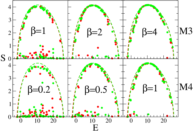
Figure 5: Dependence of entropy $S$ on energy $E$ at time $t=10^{6}$ for two disorder realisations in 2d models $M3$ (top row) and $M4$ (bottom row). Here $f=1$, $W=2$, the lattice has $8\times 8$ sites, the averaging is done in a time interval $\delta t=t/10$. Points show the numerical data, dashed curves show the corresponding theoretical Gibbs distributions, the values of $\beta$ are directly given on the panels.

We take here a relative large value of a static field $f=1$ having in mind to model the evolution of the nonlinear Schödinger equation in a Sinai billiard. Of course, the model $M3$ is only an approximation of this physical system. The obtained results resemble those found for 1d models. At weak nonlinearity we have a a large fraction of non-thermalized modes while for $\beta\geq 2$ (in $M3$) and $\beta\geq 1$ (in $M4$) we find that practically all initial conditions with linear eigenmodes follow the $S(E)$ curve given by the quantum Gibbs anzats.

• 

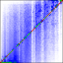
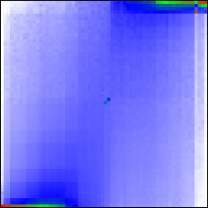
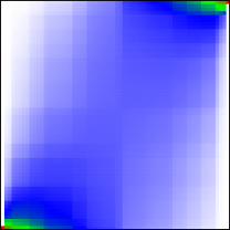
Figure 6: Time and disorder averaged probabilities $\rho_{m}(m^{\prime})$ in mode $m$ for initial state in mode $m^{\prime}$ for 2d model $M3$ with $f=1$, $W=2$, the lattice has $8\times 8$ sites; the probability is proportional to color changing from maximum (red) to minimum (white). Panels show the indexes $1\leq m^{\prime}\leq N$ in $x$-axis and $1\leq m\leq N$ in $y$-axis. The average is done over $N_{d}=10$ disorder realisations using the time interval $\delta t=10^{6}$ starting from time $t=10^{6}$. Left and center panels show the cases with $\beta=1$ and $\beta=4$ respectively while right panel illustrates theoretical values obtained from the quantum Gibbs distribution (10).

A more detailed comparison between the numerically obtained probabilities $\rho_{m}$ and the probabilities given by the Gibbs anzats is shown in Fig. 6. For a given disorder realisation we start from linear eigenmode $m^{\prime}$ and numerically determine the time averaged probability $\rho_{m}$ in each of $N$ linear modes. In addition $\rho_{m}$ are averaged over 10 disorder realisations. The numerical results at $\beta=1,4$, $W=2$, $N=32$ are compares with the theoretical probabilities of Gibbs anzats obtained for the same disorder realisations (Fig. 6). We see that for $\beta=1$ (left panel) there is a significant probability to find non-thermalized modes well visible as a high density near the diagonal. However, for $\beta=4$ we have a good agreement with the probability distribution of Gibbs anzats.

6 Results for 1d Klein-Gordon lattice model

The above lattice models have two exact integrals of motion being the energy of the system and the total probability. These models are obtained from a nonlinear Schödinger equation and hence the appearance of the quantum Gibbs distribution can be viewed as somewhat natural result with the dynamical thermalization over quantum linear modes produced by a moderate nonlinearity. Due to that it is interesting to study the case of KG model which have only one energy integral.

• 

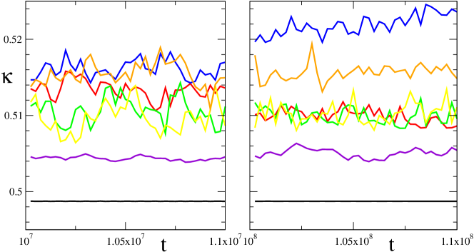
Figure 7: Time evolution of the norm of $\rho$ averaged in time, given by $\kappa=\sum_{m}\overline{|C_{m}|^{2}}$. The averaged time $\delta t$ and starting time $t$ are $\delta t=2.5\times 10^{5}$ and $t\sim 10^{7}$ for left panel and $\delta t=2.5\times 10^{6}$ and $t\sim 10^{8}$ for right panel. The initial states are taken as normalized eigenstates of the linear system with $m=1,6,11,16,21,26,31$ (with corresponding colors: black, red, blue, green, yellow, orange, violet) for KG model at $N=32$, $W=2$, $f=1/8$ and $\beta=1$.

To understand the properties of KG model we note that the eigenmodes of its linear part are described by the same linear equations as 1d Anderson model (see the correspondence description in [18]). To explore this correspondence in a deeper way we determine the eigenmodes of displacements $u_{lm}$ with eigenfrequencies $\omega_{m}^{2}$. The time evolution of the nonlinear KG equation (9) is solved numerically up to times $t=10^{8}$ for different disorder realizations. At the initial time $t=0$ we start with $u_{l}(t=0)=u_{lm}$ and $p_{l}(t=0)=0$ ($\sum_{l}u_{lm}^{2}=1$). During the time evolution we compute the expansion coefficients $C_{m}(t)=\sum_{l}u_{l}(t)u_{lm}$. From them we determine the time averaged norm $\kappa=\sum_{m^{\prime}}\overline{|C_{m^{\prime}}|^{2}}$ where the averaging is done over a time interval $\delta t$ around time $t$. The dependence of $\kappa$ on time for various initial eigenmodes $m$ is shown in Fig. 7. We see that even at very large times $\kappa$ remains approximately constant with variations remaining on a level of $1-2$ percents. On average we have $\kappa\approx 1/2$ since a half of energy is concentrated in the kinetic part which is taken at zero at $t=0$. Since $\kappa$ remains an approximate integral of motion we define the probabilities $\rho_{m}=|C_{m}|^{2}/\kappa$ so that their sum is normalized to unity at a given moment of time $\sum_{m}\rho_{m}=1$. With such a definition of $\rho_{m}$ we compute the entropy $S$ of the KG model via the usual relation (11). Of course, this normalization does not affect the actual values of $u_{l}(t)$ computed during the time evolution. The energy $E$ is the total energy of (9) with the initial state being the linear eigenmode $u_{lm}$ and $p_{l}=0$. The energies of linear modes are $\epsilon_{m}=\omega_{m}^{2}/2$. With these conditions we can test the validity of the Gibbs anzats for the KG model.

• 

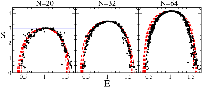
Figure 8: Dependence of entropy $S$ on energy $E$ at time $t=10^{8}$ for $7$ disorder realisations in the KG model at $W=2,\beta=1,f=0$. The averaging is done in the time interval $\delta t=10^{6}$. The lattice size is $N=20,32,64$ (from left to right respectively). Points show the numerical data, dashed curves show the quantum Gibbs distributions for each disorder realization. Solid blue line represents maximum entropy state given by a uniform distribution.

The results for the standard parameters of the KG model at $\beta=1$, $f=0$, used in [18], are shown in Fig. 8. At small lattice size $N=20$ the fluctuations are present in $S(E)$ dependence but at larger sizes $N=32,64$ we find a good agreement of numerical data with the quantum Gibbs anzats.

• 

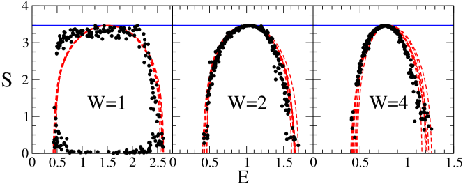
Figure 9: Same as in Fig. 8 for $W=1,2,4$ at $\beta=1$, $f=0$, $N=32$; other parameters are as in Fig. 8.

The dependence on effective disorder strength $W$ is shown in Fig. 9 for the standard parameters of KG model $\beta=1,f=0$. We see that at disorder $W=1$ there is a significant fraction on non-thermalized states. We attribute this to the fact that, in 1d Anderson model at such $W$, the localization length $\ell\approx 96$ becomes much larger than the system size and the linear modes cross the system practically in a ballistic way leading to a different onset of chaos. For $W=2,4$ we find a good agreement with the Gibbs anzats.

• 

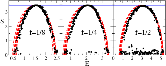
Figure 10: Same dependence $S(E)$ as in Fig. 9 for $W=2,\beta=1,N=32$ in KG model and different $f$ shown directly in panels; here $t=10^{8}$, $\delta t=10^{6}$, data are shown for $8$ disorder realisations.

The dependence of $S(E)$ on $f$ for a fixed $\beta=1$, $W=2$ is shown in Fig. 10. As for the DANSE type models discussed above we find that at large $f$ the fraction of non-thermalized modes becomes significant. The physical reasons are the same: the average spacing between linear modes becomes larger than the nonlinear coupling and the system starts to approach an integrable regime.

• 

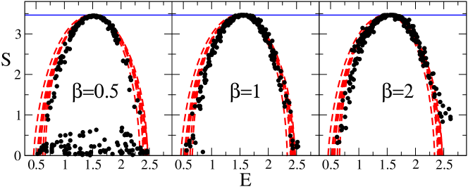
Figure 11: Same as in Fig. 10 for $f=0.125,W=2,N=32$ and $\beta$ shown directly in the panels; same $8$ disorder realisations.

The dependence of $S(E)$ on nonlinear parameter $\beta$ at fixed $f=0.125,W=2$ is shown in Fig. 11. At $\beta=0.5$ we still have non-thermalized modes in the Kolmogorov-Arnold-Moser intergability regime. The numerical data are in a good agreement with the Gibbs anzats at $\beta=1$ while at $\beta=2$ the deviations become slightly visible. The deviations become larger for $\beta=4$ (data not shown). This happens since at large $\beta$ the nonlinear part of Hamiltonian is not weak or moderate and, hence, it leads to appearance of significantly nonlinear effects including breathers and other phenomena. It is possible that the classical energy equipartition over linear modes will appear at such larger nonlinearities. Thus we find that the quantum Gibbs anzats is valid inside a certain finite range of nonlinearity $\beta_{min}<\beta<\beta_{max}$.

• 

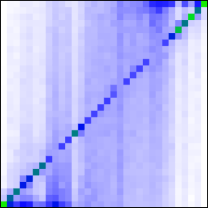
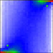
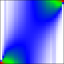
Figure 12: Same probability distribution $\rho_{m}(m^{\prime})$ as in Fig. 6 shown for the KG model with parameters $f=0.125,W=2,N=32$ at $t=10^{8}$, $\delta t=10^{6}$, and $5$ disorder realisations. Left and center panels show the cases with $\beta=0.5$ and $\beta=1$ respectively while right panel illustrates theoretical values obtained from the quantum Gibbs distribution (10).

At moderate nonlinearities $\beta=1$ we find that not only the curve $S(E)$ is well described by the Gibbs anzats but also the probabilities $\rho_{m}(m^{\prime})$. This fact is illustrated in Fig. 12 where the probability distributions $\rho_{m}(m^{\prime})$, shown in color, are in a good agreement with the quantum distribution of probabilities given by the theoretical Gibbs distribution. At small $\beta=0.5$ we have non-thermalized states with a higher density at the diagonal similar to Fig. 6.

7 Discussion

In this work we studied numerically the time evolution in various types of classical lattices with moderate nonlinearities. We show that at moderate values of nonlinear parameter $\beta_{min}<\beta<\beta_{max}$ and at large time scales the nonlinear interactions between linear lattice modes creates a steady state quantum probability distribution over energies of linear modes. This steady state probability distribution is well described by the quantum Gibbs anzats (10) being drastically different from the classical steady state energy equipartition over linear modes expected from classical thermalization picture. In a certain sense the nonlinear term generates a dynamical thermalization in the whole system with the emergence of the quantum Gibbs distribution. The appearance of such a quantum statistics takes place not only in the lattices with a discrete Schödinger equation (DANSE type), where energy and norm are both conserved, but also in other type of lattices which have only one exact integral of energy. We argue that in the latter case there is an approximate conservation of norm that makes again such nonlinear lattices to be similar to the DANSE type case. The emergence of the quantum Gibbs anzats in nonlinear lattices with only one energy integral of motion allows us to make a conjecture that the quantum Gibbs anzats is a generic phenomenon typical for many-mode lattices with weak or moderate nonlinearities. Indeed, a system of linear oscillators is effectively equivalent to a certain effective Schrödinger equation and thus a nonlinear interaction of modes can drive a generic lattice to the quantum Gibbs distribution via dynamical thermalization. We think that the further analysis of dynamical thermalization in nonlinear classical lattices is of fundamental importance for a deeper understanding of onset of ergodicity and thermalization in such systems.

We hope that the phenomenon of dynamical thermalization described here can be tested in experiments with cold atoms in optical lattices (e.g. like in [32, 47]), nonlinear photonic lattices (e.g. like in [30, 31]) or optical fiber arrays [50, 51, 52] which seems for us to be especially promising.

References

References

- [1] Plank M 1901 Annalen der Physik 309(3) 553
- [2] Gibbs J W 1902 Elementary Principles in Statistical Mechanics, developed with especial reference to the rational foundation of thermodynamics (New York: Charles Scribner’s Sons, London: Edward Arnold)
- [3] Landau L D and Lifshitz E M 1976 Statistical Mechanics (Nauka, Moscow; in Russian)
- [4] Mayer J E and Goeppert-Mayer M 1977 Statistical Mechanics (John Wiley & Sons, N. Y.)
- [5] Arnold V and Avez A 1968 Ergodic problems in classical mechanics (Benjamin, N. Y.)
- [6] Kornfeld I P, Fomin S V and Sinai Y G 1982, Ergodic Theory (Springer, N. Y.)
- [7] Chirikov B V 1979, Phys. Rep. 52 263
- [8] Lichtenberg A and Lieberman M 1992 Regular and Chaotic dynamics (Springer, N.Y.)
- [9] Fermi E, Pasta J, Ulam S and Tsingou M 1955 Los Alamos Report No.LA-1940 (unpublished)
- [10] Fermi E 1965 Collected papers vol.2 (University of Chicago Press,Chicago)
- [11] Campbell D K, Rosenau P and Zaslavsky G (eds.) (2005) A focus issue on “The Fermi-Pasta-Ulam problem - The First 50 Years” Chaos 15(1) 1
- [12] Gallavotti G (ed.) 2008 The Fermi-Pasta-Ulam problem 728 (Springer Lect. Notes in Physics, Berlin)
- [13] Shepelyansky D L 1993 Phys Rev Lett 70 1787
- [14] Anderson P W 1958 Phys Rev 109 1492
- [15] Molina M I 1998 Phys Rev B 58 12547
- [16] Pikovsky A S and Shepelyansky D L (2008) Phys Rev Lett 100 094101
- [17] Flach S, Krimer D O and Skokos C 2009 Phys Rev Lett 102 024101
- [18] Skokos C, Krimer D O, Komineas S and Flach S (2009) Phys Rev E 79 056211
- [19] Garcia-Mata I and Shepelyansky D L 2009 Phys Rev E 79 026205
- [20] Skokos C and Flach S 2010 Phys Rev E 82 016208
- [21] Lapteva T V, Bodyfelt J D, Krimer D O, Skokos C and Flach S 2010 Europhys Lett 91 30001
- [22] Johansson M, Kopidakis G and Aubry S 2010 Europhys Lett 91 50001
- [23] Mulansky M and Pikovsky A 2010 Europhys Lett 90 10015
- [24] Pikovsky A and Fishman S 2011 Phys Rev E 83 025201
- [25] Mulansky M and Pikovsky A 2013 New J Phys 15 053015
- [26] Skokos C, Gkolias I and Flach S 2013 e-print arXiv:1307.0116
- [27] Wang W-M and Zang Z 2008 e-print arXiv:0805.3520
- [28] Bourgain J and Wang W-M 2008 J Eur Math Soc 10 1
- [29] Fishman S, Krivolapov Y and Soffer A 2012 Nonlinearity 25 R53
- [30] Schwartz T, Bartal G, Fishman S and Segev M 2007 Nature 446 52
- [31] Lahini Y, Avidan A, Pozzi F, Sorel M, Morandotti R, Chirstodoulis D N and Silberberg Y 2008 Phys Rev Lett 100 013906
- [32] Lucioni E, Deissler B, Roati G, Zaccanti M, Moduggno M, Larcher M, Dalfovo F, Inguscio M and Modugno G 2011 Phys Rev Lett 106 230403
- [33] Mulansky M, Ahnert K, Pikovsky A and Shepelyansky D L 2009 Phys Rev E 80 056212
- [34] Kottos T and Shapiro B 2011 Phys Rev E 83 062103
- [35] Shepelyansky D L 2012 Eur Phys J B 85 199
- [36] Zakharov V E, L’vov V S and Falkovich G 1992 Kolmogorov spectra of turbulence (Springer-Verlag, Berlin)
- [37] Nazarenko S 2011 Wave turbulence (Springer-Verlag, Berlin)
- [38] Garcia-Mata I and Shepelyansky D L 2009 Eur Phys J B 71 121
- [39] Evers F and Mirlin A D 2008 Rev Mod Phys 80 1355
- [40] Dalfovo F, Giorgini S, Pitaevskii L P and Stringari S 1999 Rev Mod Phys 71 463
- [41] Shepelyansky D L 1997 Nonlinearity 10 1331
- [42] Rasmussen K O, Cretegny T, Kevrekidis P G and Gronbech-Jensen N 2000 Phys Rev Lett 84 3740
- [43] Johansson M and Rasmussen K O 2004 Phys Rev E 70 066610
- [44] Rumpf B 2004 Phys Rev E 69 016618
- [45] Tolman R C 1918 Phys Rev 11 261
- [46] Henry B I and Szeredi T 1995 J Stat Phys 78 1039
- [47] Braun S, Ronzheimer J P, Schreiber M, Hodgman S S, Rom T, Bloch I and Schneider U 2013 Science 339 52
- [48] Carati A and Galgani L 2000 Physica A 280 106
- [49] Chirikov B V and Shepelyanskii D L 1982 Sov J Nucl Fiz 36 908
- [50] Aceves A B, Luther G G, Angelis C D, Rubenchik A M and Turitsyn S K 1995 Phys Rev Lett 75 73
- [51] Turitsyn E G, Falkovich G, El-Taher A, Shu X, Harper P and Turitsyn S K 2012 Proc R Soc A 468 2496
- [52] Turitsyn S K, Rubenchik A M, Fedoruk M P and Tkachenko E 2012 Phys Rev A 86 031804(R)