UPDATED PHOTOMETRY AND ORBITAL PERIOD ANALYSIS FOR THE POLAR AM HERCULIS (catalog ) ON THE UPPER EDGE OF THE PERIOD GAP

Abstract

Twenty-one new optical light curves, including five curves obtained in 2009 and sixteen curves detected from the AAVSO International Database spanning from 1977 to 2011, demonstrate 16 new primary minimum light times in the high state. Furthermore, seven newly found low-state transient events from 2006 to 2009 were discovered, consisting of five Gaussian-shaped events and two events with an exponential form with decay timescales of $<$0.005 days; these timescales are one order of magnitude shorter than those of previous X-ray flare events. In the state transition, two special events were detected: a ”disrupted event” with an amplitude of $\sim$ 2 mag and a duration of $\sim$ 72 minutes and continuing R-band twin events larger than all known R-band flares detected in M-type red dwarfs. All 45 available high-state data points spanning over 35 yr were used to construct an updated O-C diagram of AM Herculis (catalog ), which clearly shows a significant sine-like variation with a period of 12-15 yr and an amplitude of 6-9 minutes. Using the inspected physical parameters of the donor star, the secular variation in the O-C diagram cannot be interpreted by any decided angular momentum loss mechanism, but can satisfy the condition $\tau_{\dot{\rm M}_{2}}\simeq\tau_{\rm KH}>>\tau_{\dot{\rm R}_{\rm 2}}$, which is required by numerical calculations of the secular evolution of cataclysmic variables. In order to explain the prominent periodic modulation, three plausible mechanisms spot motion, the light travel-time effect, and magnetic active cycles are discussed in detail.

1 Introduction

Polars, a subtype of magnetic cataclysmic variables (MCVs), play an important role in the study of interactions between two components. Since the accretion disk has been broken up by the primary, highly magnetic white dwarf, mass transfer may be seen more clearly for polars (see Warner, 1995, chap.6). Tapia (1977) gives the magnetic field intensity of the white dwarf AM Herculis (catalog ), $B_{\rm WD}\sim 200$ MG, which is apparently higher than the 30 MG and 14 MG values reported by Schmidt et al. (1983) and Wickramasinghe & Martin (1985), respectively. More recent papers have proposed that $B_{\rm WD}$ should be $\sim 14$ MG (e.g. Bailey et al., 1991; Campbell et al., 2008), in good agreement with the value reported previously by Wickramasinghe & Martin (1985). AM Herculis (catalog ) is the prototypical polar star that has been monitored extensively in optical bands (e.g. Szkody & Brownlee, 1977; Young & Schneider, 1979; Crosa et al., 1981; Hutchings et al., 2002; Kafka et al., 2005a; Terada et al., 2010). A typical feature in its optical flux is two distinct photometric states: a high state with V $\sim$ 13.5 mag and a low state with V $\sim$ 15.5 mag. This phenomenon in polars is commonly attributed to variations in the mass transfer rate from the secondary star. The high state is regarded as the normal accreting state with an average mass accretion rate of $\sim 10^{-10}$ M_⊙yr^-1 (Gänsicke et al., 2001, 2006). As for the low state, Livio & Pringle (1994) proposed a starspot model in which the temporary cessation of mass transfer through the inner Lagrange (L1) point because of the migration of the starspot on the surface of the mass-donor star presumably causes the violent drop in the accretion luminosity. Then, the accretion rate would decrease to an extremely low level of $\leq$10^-12 M_⊙yr^-1, which may result from the stellar wind of the late-type secondary star (Hessman et al., 2000; Gänsicke et al., 2006). Except for the starspot model, Wu & Kiss (2008) proposed that the variations in the magnetic field configuration of the binary system can also result in the alternation of the two states. At the present time, it is therefore still an open question as to the mechanism of high/low states in polars (e.g. Kafka et al., 2005a; Kafka & Hoard, 2009).

The observed periodic modulations in the optical light curves of AM Herculis (catalog ) are thought to be the consequence of the self-eclipse of the accretion regions or part of the heated material surrounding white dwarf (Bailey & Axon, 1981; Crosa et al., 1981; Mazeh et al., 1986; Gänsicke et al., 2001). The light minimum in a typical high-state light curve of AM Herculis (catalog ) has a broad duration of $\sim 0.6P_{\rm orb}$ (e.g. Szkody & Brownlee, 1977; Olson, 1977; Bailey & Axon, 1981). Considering that the cyclotron emission near the polar(s) of white dwarfs may be a dominant source of the modulations in the V- and R-bands, Young & Schneider (1979) pointed out that the self-eclipse feature in photometric light curves has a stable modulation period, which is almost identical to the orbital period, in spite of the cycle-to-cycle variations (Szkody et al., 1980; Gänsicke et al., 2001). Based on this stability, many light minimum times from the ultraviolet to the infrared in both luminosity states have been obtained (e.g. Szkody & Brownlee, 1977; Priedhorsky & Krzeminski, 1978; Mazeh et al., 1986; Hutchings et al., 2002; Kalomeni & Yakut, 2008). In addition, there are many ephemerides representing different periodic modulation signals. For example, the magnetic ephemeris is defined by the periodic time point when the sign of the circular polarization crosses zero (Tapia, 1977; Heise & Verbunt, 1988). In addition, all optical light minimum times obey the original optical photometric ephemeris derived $\sim 35$ yr ago (Szkody & Brownlee, 1977); not all the times of the minima depend strongly on wavelength (Hutchings et al., 2002). Initially, Mazeh et al. (1986) carried out an O-C analysis and found that the variations in the O-C diagram are possibly caused by the oscillations of the white dwarf magnetic pole relative to the binary system line of centers (Crosa et al., 1981; Campbell, 1985). However, the following O-C diagrams for the high-state data alone indicated that its orbital period is almost constant (Kafka et al., 2005a). More recently, Kalomeni & Yakut (2008) argued that the ascending O-C curve, which is totally different from the previous O-C analyses, is a result of mass transfer from the low-mass red dwarf to the massive white dwarf. This assertion may imply that AM Herculis (catalog ) would become a detached binary system in the future. So far, there is not a common conclusion for the cause of the O-Cs of the primary light minima in the high state.

In this paper, the optical photometry of AM Herculis (catalog ) in low/high states from our observations and from the American Association of Variable Star Observers (AAVSO) is presented in Section 2. All collected data extend the time baseline of the O-C diagram to 35 yr. In Section 3, Kafka et al. (2005a) photometric ephemeris of AM Herculis (catalog ) is corrected based on our new photometric data. Then, we analyzed the updated O-C diagram for all primary high-state minima in Section 4. Section 5 includes a discussion of the seven transient events and the possible explanations for the new O-C diagram.

2 Data ACQUISITION/REDUCTION

2.1 Photometeries

An AM Herculis (catalog ) photometric campaign was carried out from April to October 2009 using the three ground-based optical telescopes in China: the 60 cm and 1.0 m Ritchey-Chretien-Coude reflecting telescopes at Yunnan Astrophysical Observatory and the 85 cm Cassegrain telescope at Xinglong Observing Station of National Astronomical Observatories. The details of the photometry for AM Herculis (catalog ) can be seen in Table 1. All images were reduced using PHOT (measuring magnitudes for a list of stars) in the aperture photometry package of IRAF. We chose two nearby photometric standards for AM Herculis (catalog ), AM Her-2 and AM Her-15, to be the comparison and the check star in our observations, respectively (Henden & Honeycutt, 1995). The magnitude differences between the comparison and the check star are represented by the dotted lines in Figures 1(l), (m), (n). Figures 2(e) and (f) suggest that our photometry was carried out in good seeing and that the observed variations in the light curves are genuine and believable.

The three primary CCD minimum times were derived from the high-state differential light curves shown in Figures 1(l), (m), and (n) using a least-squares fitting method to a parabolic curve. The fitting errors and the time resolution of the CCD observations were combined to estimate the uncertainties of the minimum times. The other two low-state light curves are shown in Figures 2(e) and (f) for the analysis of transient events in Section 4.1. Additionally, the two white-light light curves, i.e., Figures 1(n) and 2(e), are marked by the letter N in the top-right corner of plots. Besides the positive color indexes, i.e., B-V $\sim$ 0.5 and V-R $\sim$ 0.6 (e.g. Bailey et al., 1977; Priedhorsky et al., 1978a; Bailey & Axon, 1981), and the flat B light curves (e.g. Olson, 1977; Bailey et al., 1977; Mazeh et al., 1986; Gänsicke et al., 2001), the total spectral energy distribution derived by Priedhorsky et al. (1978b) and Bailey & Axon (1981) demonstrate that the unfiltered photometries of AM Herculis (catalog ) are mainly dominated by radiation in the long-wavelength band and beyond.

2.2 Light Minimum Times from the Literature

The photometric ephemeris in the far-ultraviolet band derived by Hutchings et al. (2002) is different from that derived completely in the visual band (Szkody & Brownlee, 1977; Kafka et al., 2005a). The offset of light minimum times between the FUV/X-ray and optical bands is almost up to half an orbital period (e.g. Hearn & Richardson, 1977; Mazeh et al., 1986; Hutchings et al., 2002). Therefore, Kalomeni & Yakut (2008) were not justified in combining the average of the light minimum times in the FUV with those in the optical for their O-C analysis. In this paper, all 29 available photometric data points in HJD, including the data extracted from the literature, are listed in Table 2. Since AM Herculis (catalog ) has two distinct photometric states corresponding to different accretion configurations, we reexamined the photometric states of all 29 timing datasets.

Note that the three light minimum times obtained by Kalomeni & Yakut (2008) present significant deviations of $\sim 0.5$ $P_{\rm orb}$ from the photometric ephemerides derived by Szkody & Brownlee (1977) and Kafka et al. (2005a). Although these light minimum times may be the times of secondary minima, Kalomeni & Yakut (2008) never made any special mention of them. Hence, these times cannot be included in our O-C analysis because of the instability of secondary minima (Bailey et al., 1977; Szkody et al., 1980; Kafka et al., 2005a).

2.3 Data from AAVSO

The AAVSO is famous for its abundant information and data on variable stars. The data from the AAVSO International Database (AAVSOID) are well calibrated and accurate. Currently, there are a total of 33,292 observations for AM Herculis (catalog ) recorded in the AAVSOID, and this number is always growing. Thus, it is necessary to take full advantage of the data in the AAVSOID. Based on this database, we have extracted 16 available optical light curves. Twelve light curves covering at least one primary minimum are listed in Figures 1(a)-(k), and the other four light curves with transient events are listed in Figure 2. The same parabolic fitting method and the method of estimating the timing uncertainty used in Section 2.1 were also applied to calculate the primary minimum times and the corresponding errors. The multi-band observations shown in Figure 1(c) clearly suggest a high consistency in the primary minimum timings of different optical bands.

Kafka & Hoard (2009) have pointed out that there are three subtypes in the high state of AM Herculis (catalog ) (i.e., a normal high state and another two newly defined high states labeled A and B in their Figure 1). Accordingly, we checked the photometric states of all 16 light curves in detail. Figures 1(c) and (d) show light curves in a failed high state and Figures 1(e)-(i) show data in a faint high state. All of the primary minimum times in three subtypes are included in our timing analysis due to the striking similarity of their light curves (Kafka & Hoard, 2009). Finally, the 13 primary minimum times in the high state are measured from the AAVSOID. Since the timing system of the data used in the AAVSOID is JD, we have converted this timing system to HJD for consistency with the literature.

3 EPHEMERIS and O-C ANALYSIS

All of the light curves shown in Figure 1 show that the primary minima of AM Herculis (catalog ) are stable in spite of the observed cycle-to-cycle changes in the profiles. The recent photometric ephemeris of Kafka et al. (2005a),

$$T_{0}=HJD\ 244603.403(5)+0.12892704(1)\ E,$$ (1)

is not only an updated ephemeris derived from high-state photometric data spanning more than 10 yr, but is also a spectroscopic ephemeris defining phase zero at the inferior conjunction of the secondary star. Compared with the old photometric ephemeris (Szkody & Brownlee, 1977), the accumulated time error has grown up to 11 minutes. In order to reduce the accumulated error in the timing analysis, we chose the recent ephemeris of Kafka et al. (2005a) to calculate O-Cs for all 45 high-state light minimum times. Considering that the uncertainty of the epoch in Equation (1) is 0.005 days (i.e., $\sim$ 7.2 minutes), which can result in a large scatter in the O-C analysis, we revised this ephemeris and improved its precision based on the 45 high-state data spanning 35 yr. Since there are 21 light minimum times published in the literature that lack corresponding uncertainties, we adopted a unified uncertainty, 8.8 days $\times 10^{\rm-4}$, which was estimated from the arithmetic mean of the other 24 known errors. The corrections for the new epoch and orbital period of AM Herculis (catalog ) listed in Table 3 were calculated from a simple linear fit to the high-state O-Cs. Thus, a corrected photometric ephemeris, corresponding to the linear fitting case listed in Table 3, was derived as:

$$T_{0}=HJD\ 2446603.401658(99)+0.1289271368(17)\ E,$$ (2)

with a variance of 4.3 days $\times 10^{\rm-3}$. The difference in epoch between the new and old ephemerides is only $\sim$ 2 minutes. However, the precision of the new epoch has been improved by a factor of over 50. In addition, the other four nonlinear fitting formulae - linear-plus-sinusoidal, constant-plus-sinusoidal, quadratic-plus-sinusoidal, and quadratic-plus-LITE listed in Table 3 - are used to describe the O-C diagram of AM Herculis (catalog ) (see Figure 4), where the formulae refer to the solid lines, dotted lines, short lines, and long dashed lines, respectively. A Levenberg-Marquadt algorithm was used to carry out the three nonlinear least-squares fitting routines with strict sinusoidal term. The reduced $\chi^{\rm 2}$ in the three cases were all near unity, and the F-test proposed by Pringle (1975) confirms their high confidence levels, over 99%. In order to further verify the existence of quadratic and periodic variations, we utilized an improved Nelder-Mead simplex algorithm, which is based on the famous nonlinear optimization method first proposed by Nelder & Mead (1965). We used this algorithm to analyze the high-state O-C diagram. The fitting formulation is described by Irwin (1952):

$$\left\{\begin{array}[]{l}O-C=\alpha+\beta E+\gamma E^{2}+\tau_{\rm LITE}\\ \\ \tau_{\rm LITE}=\frac{\kappa}{\sqrt{1-e^{2}\cos^{2}\Omega}}[\frac{1-e^{2}}{1+e\cos\nu}\sin(\nu+\Omega)+e\sin\Omega]\\ \\ \tan{\frac{\nu}{2}}=\sqrt{\frac{1+e}{1-e}}\tan\frac{EE}{2}\\ \\ M=EE-e\sin{EE}\\ \\ M=\frac{2\pi}{P_{3}}(t-T_{0})\\ \end{array}\right.$$ (3)

where E is the cycle and $\kappa$, e, $\Omega$, $\nu$, M, EE, $T_{0}$, $P_{3}$ and t are the semi-amplitude, eccentricity, longitude of periastron, true anomaly, mean anomaly, eccentric anomaly, time of periastron passage, orbital period of the third body, and the minimum time, respectively. In all, there are eight parameters ($\alpha$, $\beta$, $\gamma$, $\kappa$, $e$, $\Omega$, $T_{0}$ and $P_{3}$) in Equation (3). We have performed three important parameter searches for e, $P_{3}$ and $\gamma$. In each iteration, the searched parameters are fixed in turn, but changed with a small given step. Within the reasonable parameter range, we obtained a reduced $\chi^{2}_{\rm\zeta}$ as a function of the different parameter values. As can be seen in Figure 3, the clear minimum values for the three searched parameters are e(min) $\sim$ 0.5, $P_{3}$(min) $\sim$ 5400 days, and $\gamma$(min) $\sim\rm-10^{-11}$, respectively. All three minimum values are consistent with the final optimized parameters listed in Table 3, to some extent. The output of the Nelder-Mead simplex algorithm was assigned to be an initial input parameter for the Levenberg-Marquadt algorithm for estimating the corresponding parameter errors. Note that Figure 3 illustrates some important facts: the eccentricity can be acceptable as long as e $<$ 0.5, the optimized quadratic coefficient $\gamma$ is extremely close to zero, and it is hard to find the best cyclical period within a range of 5000-5400 days. Hence, the true errors of the three parameters may be larger than those listed in Table 3. It is interesting to note that the period and amplitude of the sinusoidal variation in all four cases are almost identical. Therefore, a periodic modulation with a period of 12-15 yr and an amplitude of 6-9 minutes in the O-C diagram of AM Herculis (catalog ) cannot be neglected. For the first time, a sinusoidal-like oscillation shown in Figure 4 is found for the prototypical polar AM Herculis (catalog ). In Section 4.2, we will discuss the possible secular orbital period variation of AM Herculis (catalog ) in light of the above timing analysis.

4 Discussion

4.1 Transient Events

Low-state transient events are common phenomena in polars (e.g. Ramsay et al., 2004; Pandel & Córdova, 2005; Araujo-Betancor et al., 2005). For the prototypical polar AM Herculis (catalog ), there are plenty of low-state transient events (e.g. Shakhovskoy et al., 1993; Bonnet-Bidaud et al., 2000; Kafka et al., 2005b; Kalomeni & Yakut, 2008; Kafka & Hoard, 2009; Terada et al., 2010). In this paper, seven new low-state transient events are detected. Figures 2(a)-(d) show the prominent events in the light curves acquired during the 2006 low state and the end of the high-to-low state transition in early 2008 August. Figures 2(e) and (f) show the events in the egress branches of light minima acquired during the beginning of the low-to-high state transition in early 2009 April. The two light curves in the 2006 low state lie right in the duration of the short flares labeled ”C” in Kafka & Hoard (2009). All of the light curves in Figure 2 phased by the ephemeris in Equation (2) show that the transient events are confined to a phase space between 0.0 and 0.5. Although all seven events spanning 2006 to 2009 were not observed in a series of sequential nights, every two light curves were obtained in the same season of the same year. From top to bottom, the seven events clearly demonstrate a distinct phase drift as a function of time. It is interesting that the direction of the phase drift in the three events of 2009 are opposite to the direction of the phase drifts of the previous four events. Additionally, the 9 mag excesses observed by Kalomeni & Yakut (2008) were also scattered in orbital phase. Hence, the detected phase drift in Figure 2 may imply that the low-state events of AM Herculis (catalog ) likely have no phase dependence, which further supports the distribution of the flaring events in the long-term RoboScope data (Kafka et al., 2005b).

Among the seven events, there are two special optical events with striking exponential profiles shown in Figures 2(d) and (e). These events resemble the X-ray flare event observed on 2008 October 30 by Suzaku (Terada et al., 2010). All three optical transient events were detected in a short-duration low state from 2008 August to 2009 April. The striking similarity in profile between optical and X-ray events may imply a similar driving mechanism. An offset exponential function similar to that used in the X-ray event (Terada et al., 2010),

$$F=F_{0}+Ae^{-\frac{p-p_{0}}{\tau_{\rm flare}}},$$ (4)

is used to describe the transient events in Figures 2(d) and (e), where F0, A, p, $p_{0}$ and $\tau_{\rm flare}$ are the magnitude of the post event, the amplitude of the event, the orbital phase, the initial orbital phase of the event, and the decay constant in phase units, respectively. The parameters for both events are listed in Table 4. Assuming that the end phase of the event corresponds to a magnitude difference of 0.1 mag between the event and the post event, the duration of the event $\Psi$ can be estimated. The decay constant $\tau_{\rm flare}$ for both optical events is less than for the X-ray flare event. This result may indicate that transient events for polars with similar exponential forms are high-energy events. According to Equations (2) and (3) in Terada et al. (2010), the smaller flare cannot yet be regarded as the cooling timescale of the thermal plasma. Considering that both optical events occurred near phase zero, in accordance with the phase of the X-ray flare event (i.e., $\sim$ 0.1), the transient events in exponential form may not only be caused by a same mechanism, but may also come from the same location.

On the other, there are five symmetric transient events (i.e., nearly equal rise and fall branches) shown in the other four light curves, which are different in shape from the V-band OPTIC flare during the 2004 low state, which had a faster rise branch than fall (Kafka et al. 2005b). A Gaussian function

$$F=F_{0}+Ae^{-(\frac{p-p_{0}}{\Gamma})^{2}},$$ (5)

where $\Gamma$ is equal to $\sqrt{2}\Psi$/6, is used to fit these transient events. Table 4 lists the details of the five events, including the lasting time, the peak phase, and the amplitude. The brightening events in Figures 2(a), (b), and (f) present typical amplitudes of 0.2-0.6 mag and durations of several tens of minutes (Bonnet-Bidaud et al., 2000; Kafka et al., 2005a, b). Although there is seemingly not any obvious transient event in the light curve observed on 2008 August 4, the violent variations in phase near $\sim$ 0.15 and $\sim$ 0.4 are distinctly alike the steep rise and fall branches of a symmetric transient event. Additionally, the light curve is flat outside the variations from $\sim$ 0.15 to $\sim$ 0.4, and seem to repeat this variation after $\sim$ 0.6. Therefore, we deduced the bold hypothesis that the low-state light curve of AM Herculis (catalog ) may hide a lot of periodic huge events, which are usually disturbed by unclear mechanisms, unfortunately. Assuming that the residual accretion in the low state of AM Herculis (catalog ) is blobby accretion (Litchfield & King, 1990; Gänsicke et al., 1995), which caused the huge 1992 event (Bonnet-Bidaud et al., 2000), it may be possible that the occasional occultation of the accretion blobs results in the two dips in the ”disrupted” plateaus of event. A Gaussian function is also used to fit its rise and fall branches, as with the other symmetric events. The best-fitting Gaussian curve denoted by the dashed line in Figure 2(c) seem to reappear in the ”disrupted” huge V-band flare event with an amplitude of $\sim$ 2 mag and a duration of $\sim$ 72 minutes. It is interesting that this ”disrupted event” is strikingly similar to the Rc-band flare event shown in Figure 4(b) of Kalomeni & Yakut (2008). However, the duration of $\sim$ 72 minutes is three times longer than that of the 1992 event (Shakhovskoy et al., 1993; Bonnet-Bidaud et al., 2000). Since this light curve was observed just at the end of the high-to-low state transition, the whole system of AM Herculis (catalog ) may be undergoing a violent adjustment from the high state to the low state. Based on the starspot-covering model near the L1 point (Livio & Pringle, 1994), this huge ”disrupted event” may be an important manifestation of the strengthening of stellar magnetic activities on the surface of the red dwarf during the end of the high-to-low state transition.

On the other hand, the two continuing R-band brightening events with similar amplitudes and durations occurring in the same egress branch of the light minimum shown in Figure 2(f) were just detected at the beginning of the low-to-high state transition. Assuming that these continuing twin transient events were induced by the residual accretion located at the magnetic pole regions of the white dwarf, they may indicate that the two poles are active right now. If this assumption is true, then the observed twin events would be strong evidence for the conclusions of Kafka & Hoard (2009): the overall high-state accretion geometry has already been established at the end of the low state. Since an explanation for the accretion events at the two poles cannot be confirmed completely at the present, the stellar activity on the secondary star should also be discussed. Most of the R-band flares in cool stars usually have low amplitudes of less than 0.15 mag, accompanied by occasional large amplitudes over 0.2 mag (e.g. Zeilik et al., 1982; Kozhevnikova et al., 2004, 2006; Nelson & Caton, 2007; Vida et al., 2009; Zhang et al., 2010). The largest R-band flare in the M-type eclipsing binary CU Cnc detected recently by Qian et al. (2012) only had an amplitude of 0.52 mag. Consequently, the successive twin events of AM Herculis (catalog ) shown in Figure 2(f) may be two continuing large R-band flare events on a M4-5 type red dwarf (Young et al., 1981; Bailey et al., 1988; Gänsicke et al., 1995; Southwell et al., 1995). This occurrence may be just a coincidence, but the eruptive prominences resulting from coronal mass ejections on the fast rotating secondary star have already been previously observed in several polars (e.g. Shafter et al., 1985; Schwope et al., 1993; Pandel & Córdova, 2002, 2005). Does this result mean that the red dwarf in polars has been affected by the magnetic white dwarf? In addition, we cannot neglect another possible interpretation that both similar events originate from different physical regions in AM Herculis (catalog ) (i.e., one is from the magnetic pole and the other is from the flare). Hence, simultaneous X-ray and optical observations are necessary in the future for identifying all of these low-state transient events in AM Herculis (catalog ).

Moreover, we noted that the two light curves observed in the 2009 low state likely show a significant modulation near phase zero. However, the top four low-state light curves in Figure 2 never present any modulation. In particular, the entire light curve in Figure 2(b) is almost flat, except for the event near phase 0.33. Since the two low-state light curves were observed at the beginning of the 2009 low-to-high state transition, their modulations may be caused by the recovered high-state accretion geometry. This result implies that the humps in Figures 2(e) and (f) near phase 0.7 with a typical amplitude of $\sim$ 0.6 mag and the extremely long phase duration of $\sim$ 0.4 (via $\sim$ 74 minutes) may be caused by the cyclotron emission region located at the accreting column(s). Our data alone cannot totally rule out the explanation of an accretion event or flare event on secondary star. In this case, AM Herculis (catalog ), with its rich series of events/bursts, could be a highly active binary system, marked by the rapid establishment of a high-state accretion geometry at the low-to-high state transition.

Except for the brightening events in Figure 2, there is a special V-shaped light minimum event with a duration of $\sim$ 15 minutes and an amplitude of $\sim$ 0.7 mag shown in Figure 1(m) occurring at a phase $\sim$ 0.6. The amplitude of this minimum is almost the same as that of the primary minimum. However, this minimum is totally different from the secondary minimum of AM Herculis (catalog ) (Szkody & Brownlee, 1977; Szkody et al., 1980; Gänsicke et al., 2001). If this minimum is regarded as a peculiar secondary minimum, then the accretion region near the magnetic pole(s) of the white dwarf would be reduced to one-fifth of its normal size and deflected $\sim$ 30^∘. away from its original location. This dramatic variation does not justify the stable high-state accretion configuration. Additionally, the two temporary plateaus near phase 0.7 and phase 0.9 with a duration of $\sim$ 9 minutes, denoted by the two dashed-dot circles in Figure 1(m), have also been detected clearly in the ingress branch of the primary minimum. Thus, it is more probable that the normal cyclotron beaming modulation cycle is disturbed coincidently by some uncertain short-duration occultations. Unfortunately, the lack of a light curve before this V-shaped minimum cannot be used to reveal more information about this peculiar minimum.

4.2 Secular Orbital Period Variations

Inspection of the lower panel of Figure 4 indicates that the two best-fitting curves seem to clearly deviate away from the data point at cycle 36254. In order to check the quadratic term, a simple quadratic function is used to fit this O-C diagram. The variance of the quadratic fitting, 4.7 days $\times 10^{-3}$, is even larger than that of the linear fitting, 4.3 days $\times 10^{-3}$. This result means that the significant level of the quadratic term is zero. Conservatively, the quadratic variation in AM Herculis (catalog ) is uncertain, based on the present 45 high-state photometric data points. However, since the orbital period of AM Herculis (catalog ) is located just at the upper edge of the period gap, further investigation may be necessary to understand the secular orbital period variations in AM Herculis (catalog ).

Considering that the physical parameters of the donor star are key for the evolution of CVs (see, e.g., Rappaport et al., 1983; Spruit & Ritter, 1983; Howell et al., 2001), we attempt to investigate its mass and radius derived by Young et al. (1981). Corresponding to a normal main sequence star with a mass of $\sim$ 0.26 M_⊙, the radius in thermal equilibrium should be Re $\sim$ 0.27 R_⊙ based on Table 15.8 of Cox (2000). Hence, the donor star of AM Herculis (catalog ), with a radius of R2 $\sim$ 0.32 R_⊙, is obviously oversized by a bloating factor $f(R_{2}/R_{e})$ $\sim$ 1.2, which is just a lower limit corresponding to the shorter width (3/4 hr) of the period gap (Howell et al., 2001). In addition, f can also be obtained from the mass and radius relations of the donor star as a function of the orbital period, as deduced by Howell et al. (2001):

$$\begin{array}[]{rl}M_{2}(P_{orb})\simeq 0.08f^{-1.95}P_{orb}^{1.3},\\ \\ R_{2}(P_{orb})\simeq 0.10f^{-0.65}P_{orb}^{1.1},\\ \end{array}$$ (6)

where M₂ and R₂ are in solar units and $P_{\rm orb}$ is in hours. In sum, the donor star of AM Herculis (catalog ), with a mass of 0.26 M_⊙ and a radius of 0.32 R_⊙, is in accordance with a description of the conventional picture of CV evolution.

In light of the best-fitting parameters of the formulae with quadratic terms listed in Table 3, the orbital period decrease rate of AM Herculis (catalog ) derived from the average of two quadratic terms is $\dot{P}_{\rm orb}\sim-7.8(\pm 1.2)\times 10^{-11}$ s s^-1 (i.e., $\dot{P}_{\rm orb}/P_{\rm orb}\sim-7(\pm 1)\times 10^{-15}$ s^-1), which is one order of magnitude lower than the previous results for AM Herculis (catalog ) (Young & Schneider, 1979; Mazeh et al., 1986). However, these results are the same order of magnitude as the results of other CVs, such as the Z-Cam type dwarf nova EM Cygni (Dai & Qian, 2010a), an old post-nova T Aurigae (Dai & Qian, 2010b), and so on. Since the masses of the white dwarf and the red dwarf in AM Herculis (catalog ) are 0.78 M_⊙ and 0.26 M_⊙, respectively (Young et al., 1981), conservation of mass transfer from the red dwarf to the massive white dwarf cannot result in the orbital period decrease. Therefore, there is no justification that the upward parabolic variation in the O-C diagram given by Kalomeni & Yakut (2008) should be regarded as the consequence of conservative mass transfer. The updated O-C diagram shown in Figure 4 spanning the 30 yr data set has refuted the pseudo upward variation. On the other hand, the average mass accretion rate of $\sim$ 10^-10 M_⊙yr^-1 for both states (e.g., Young & Schneider, 1979; Hessman et al., 2000; Townsley & Bildsten, 2003; Gänsicke et al., 2001, 2006), which is small enough to be driven only by the gravitational radiation, suggests that the mass-loss timescale of the donor, $\tau_{\dot{\rm M}_{2}}\sim 2.6\times 10^{9}$ yr, is a little shorter than its Kelvin CHelmholtz timescale, $\tau_{\dot{\rm M}_{2}}\sim 2.6\times 10^{9}$ yr. Both timescales are comparable, which may imply that AM Herculis (catalog ) is indeed approaching the period gap, according to the standard evolutionary scenario for CVs (see, e.g., Spruit & Ritter, 1983; Rappaport et al., 1983; Howell et al., 2001; Knigge et al., 2012). Using the formula of Paczyński (1971),

$$\frac{R_{\rm L_{2}}}{a}=0.462(\frac{M_{2}}{M})^{1/3},$$ (7)

where a is the binary separation and M is the combined mass of two component stars (i.e.,M = M₁+M₂), the Roche-lobe radius of the donor star can be calculated to be $R_{\rm L_{2}}\sim 0.27$ R_⊙, which is smaller than the radius of the donor star $R_{2}\sim 0.32$ R_⊙.Based on Kepler s third law, a logarithmic differentiation of Equation (7) yields:

$$\frac{\dot{R}_{\rm L_{2}}}{R_{\rm L_{2}}}=\frac{\dot{M}_{2}}{3M_{2}}+\frac{2}{3}\frac{\dot{P}_{\rm orb}}{P_{\rm orb}}.$$ (8)

Hence, $\dot{R}_{\rm L_{2}}/R_{\rm L_{2}}\simeq-1.48\times 10^{-7}$ yr^-1. Supposing that the variation of $R_{2}$ and $R_{\rm L_{2}}$ are synchronized (i.e., $\tau_{\dot{\rm R}_{2}}\simeq(\dot{R}_{\rm L_{2}}/R_{\rm L_{2}})^{-1}$), the average radius adjustment timescale of the donor star, $\tau_{\dot{\rm R}_{2}}$, can be estimated to be $6.8\times 10^{6}$ yr. This result means that $\tau_{\dot{\rm R}_{2}}\simeq 0.02\tau_{\rm KH}$. On the basis of the detailed reviews and the analytical estimates of $\tau_{\dot{\rm R}_{2}}$ for stars with a substantial convective envelope (Stehle et al., 1996; Knigge et al., 2012), this timescale amply satisfies the requirements of the sharp edges of the period gap and the well-defined cutoff at $P_{\rm min}$ in the CV distribution demonstrated by all numerical calculations of the evolution of CVs with different initial parameters (see, e.g., Paczyński & Sienkiewicz, 1983; Kolb & Ritter, 1992; Howell et al., 2001). Nevertheless, if we neglect the second term on the right side of Equation (8), then $\tau_{\dot{\rm R}_{2}}\sim 7.8\times 10^{9}$ yr would be longer than $\tau_{\rm KH}$, which contradicts the rapid convergence of CV evolution tracks at $P_{\rm orb}\approx 3$ hr (Howell et al., 2001). Thus, it is necessary to seek possible mechanism for dissipating angular momentum in AM Herculis (catalog ).

Assuming that the evolution of AM Herculis (catalog ) indeed causes the orbital period decrease with a rate similar to our observations, magnetic braking may be a possible explanation, in accordance with the standard theory of CV evolution (Robinson et al., 1981; Spruit & Ritter, 1983). A consideration of the counteraction between the mass transfer and the gravitational radiation means that magnetic braking can account completely for the observed orbital period decrease, $\dot{P}_{\rm orb}\sim-7.8(\pm 1.2)\times 10^{-11}$ s s^-1, which corresponds to an angular momentum loss rate of $\dot{J}_{\rm orb}\sim-2.9\times 10^{36}$ dyn cm. At first, we considered two magnetic braking models proposed by Rappaport et al. (1983) and Webbink & Wickramasinghe (2002), which we denote as MB1 and MB2, respectively. The MB1 model is a common magnetic braking model for non-magnetic CVs with index parameter $\gamma_{\rm MB}=3$, while the MB2 model calculates a detailed magnetic interaction in the combined magnetospheres of two component stars for magnetic CVs. Taking advantage of the physical parameters of AM Herculis (catalog ) derived by Young et al. (1981), the two models produce a similar angular momental loss rate, $\dot{J}_{\rm MB1}\sim-2.7\times 10^{35}$ dyn cm and $\dot{J}_{\rm MB2}\sim-1.7\times 10^{35}$ dyn cm, respectively, which are about one order of magnitude smaller than $\dot{J}_{\rm orb}$. As pointed out by Wickramasinghe & Wu (1994); Li et al. (1994); Webbink & Wickramasinghe (2002) and Cumming (2002), the magnetic braking in AM Herculis (catalog ) should not be cut off totally, but should rather be strongly suppressed. This suppression is due to the magnetic moment of the white dwarf, $\mu_{1}\simeq 6.2\times 10^{33}$ G cm³, corresponding to $B_{\rm WD}\sim$ 14 MG, which is smaller than the theoretical critical value, $\mu_{\rm crit}\simeq 4\times 10^{34}$ G cm³, given by Cumming (2002). Thus, magnetic braking in AM Herculis (catalog ) cannot be a viable angular momentum loss mechanism, at least not yet. Other than magnetic braking, three other mechanisms that direct mass loss from the binary system and the outflows from the Lagrangian point $L_{2}$ and the circumbinary disk, can also be involved to explain this large angular momentum loss rate. The first mechanism requires a high mass loss rate of $\sim-3.8\times 10^{-8}$ M_⊙ yr^-1. The latter two models, which have been investigated by Shao & Li (2012) in particular, can be described by the following formulae:

$$\large\begin{array}[]{l}\frac{\dot{J}_{\rm L_{2}}}{J_{\rm orb}}=(\frac{a_{\rm L_{2}}}{a})^{2}\frac{M}{M_{1}}\frac{\dot{M}_{\rm L_{2}}}{M_{2}},\\ \\ \frac{\dot{J}_{\rm CB}}{J_{\rm orb}}=\gamma_{\rm CB}\frac{M}{M_{1}}\frac{\dot{M}_{\rm CB}}{M_{2}},\\ \end{array}$$ (9)

where $a_{\rm L_{2}}$ is the distance between the mass center of the binary and the $L_{2}$ point and $\gamma_{\rm CB}$ is the fraction of the inner radius of the circumbinary disk. When we adopt the ratio $a_{\rm L_{2}}/a=1.51425$ with regard to the mass ratio $q\simeq 0.33$ from Table 1 of Mochnacki (1984) and $\gamma_{\rm CB}=1.5$ from Soberman et al. (1997), we obtain mass-loss rates of $\dot{M}_{\rm L_{2}}\sim-6.3\times 10^{-9}$ M_⊙ yr^-1 and $\dot{M}_{\rm CB}\sim-9.6\times 10^{-9}$ M_⊙ yr^-1. Therefore, all three models require inconceivably high mass-loss rates.

Unless there is another unknown but more readily available angular momentum loss mechanism that forces the evolution of AM Herculis (catalog ), this object will stay on the upper edge of the period gap for a long time and evolve slowly via gravitational radiation and severely curtailed magnetic braking. This result may support the argument that polars have their own special evolutionary track, different from the other non-magnetic CVs, as proposed by Wickramasinghe & Wu (1994); Li et al. (1994); Webbink & Wickramasinghe (2002). If this stagnation in evolution is true and common for magnetic CVs with orbital periods of 3-4 hr, then could it be possible that the period gap is caused partly by this accumulation? On the other hand, Knigge et al. (2012) proposed recently that the angular momentum loss rate for CVs below the gap is badly underestimated, and that the required angular momentum loss rate should be 2.47 times larger than that afforded by gravitational radiation. Thus, is it possible that the large $\dot{J}_{\rm orb}$ of AM Herculis (catalog ) calculated from its updated O-C diagram is caused by this mysterious angular momentum loss mechanism, since AM Herculis (catalog ) evolves into the upper edge of the gap?

4.3 Periodic Modulation

A prominent feature in the O-C diagram is the sinusoidal variation. Since the light minima photometric are attributed to the occultation of bright accretion spots by the limb of the white dwarf, a periodic spot motion may cause corresponding shifts in the light minimum times. In the eclipsing polar HU Aqr, Schwope et al. (2001) claimed a change in the spot longitude of $\sim 10^{\circ}$ between the different states.Moreover, Crosa et al. (1981) reported that the inclination of the dipolar axis of AM Herculis (catalog ) has increased by $\sim 5^{\circ}$ from 1976 to 1979. This finding may support the hypothesis of dipolar axis precession around the binary axis proposed by Bailey & Axon (1981). However, the amplitude of the modulation shown in Figure 4, $\sim$ 0.005 days (i.e., $\sim$ 0.04 P_orb), indicates that the dipolar axis should shift nearly 14^∘. within 12-15 yr, which is larger than the conclusion of Crosa et al. (1981). Thus, further evidence is needed to support this hypothesis. Moreover, a dipolar axis precession with an amplitude of $5^{\circ}$-$10^{\circ}$ will only cause a small offset in the light minimum times, $\sim 3$ minutes (i.e. $\sim$ 0.02 P_orb). This result means that more high-precision photometry is needed to clarify this spot motion mechanism.

The modulations in the O-C diagrams of many other eclipsing polars such as UZ For (Potter et al., 2011; Dai et al., 2010), DP Leo (Beuermann et al., 2011; Qian et al., 2010), and HU Aqr (Goździewski et al., 2012; Qian et al., 2011) are interpreted by the light travel-time effect, which is caused by a perturbation from a tertiary component. Since the optimized parameters of the sine-like modulation listed in Table 3 are similar for the four non-linear fitting cases, we chose a set of parameters of linear-plus-sinusoidal fitting to estimate the projected distance from the binary to the mass center of a triple system, $A_{12}\sin{i_{3}}\sim 0.89(\pm 0.02)$ AU, and the mass function of the third component, $f(M_{3})\sim 4.5(\pm 0.4)\times 10^{-3}$ M_⊙. A combined mass of 0.78 M_⊙ + 0.26 M_⊙ is used to calculate the two relationships of $M_{3}$ versus $i_{3}$ and $A_{3}$ versus $i_{3}$. Both relationships shown in Figure 5 clearly indicate that this assumed third component should be a red dwarf with a mass similar to the secondary star, as all of them are in a coplanar orbit. Its mass is close to 0.2 M_⊙, even if $i_{3}$ reaches up to $90^{\circ}$. The separation between the third body and the binary is three orders of magnitudes larger than that of the binary itself, $a\sim 0.92$ R_⊙, as long as the orbital inclination is moderate (i.e., $i_{3}>30^{\circ}$). In an eccentric orbit, $M_{3}$ and $A_{3}$ can be calculated using the following formulae (Irwin, 1952; Mayer, 1990):

$$\begin{array}[]{l}f(M_{3})=\frac{(A_{12}\sin{i_{3}})^{3}}{P^{2}_{3}}=\frac{1}{P^{2}_{3}}(\frac{173.15\kappa}{\sqrt{1-e^{2}\cos^{2}\Omega}})^{3},\\ \\ A_{3}=A_{12}\frac{M_{1}+M_{2}}{M_{3}},\\ \end{array}$$ (10)

where $A_{12}$ and $P_{3}$ are in AU and years, respectively. Although the significance level and the parameter errors listed in Table 3 suggest that quadratic-plus-LITE fitting is not an optimized description of the O-C diagram of AM Herculis (catalog ) compared with the other three cases with strict sinusoidal terms, Figure 5 obviously shows that the thin lines denoting the eccentric orbit are close to the other thick lines referring to the circular orbit, except for the small difference between the two dashed lines at high inclinations. Hence, to some extent, the eccentricity $\sim$ 0.47 never changes the dynamic feature of the third star seriously. Compared with the gravitational binding energy of the two components of AM Herculis (catalog ), the interaction between the third red dwarf and the binary system can be neglected, which means that a dynamic stable triple system can be expected. If this assumed a red dwarf indeed exists, then AM Herculis (catalog ) would be a peculiar system with an amazing configuration and its formation and evolution would be worthy of further investigation. In fact, it is hard to definitely distinguish the secondary and third components in observations since their discrepancies in the coplanar case are only in their spin velocity and reflection effect. On the other hand, the abundance of incredible and complicated transient events in AM Herculis (catalog ) may badly blur the two red dwarfs. In particular, compared with the brilliant accreting magnetic white dwarf, the observational features of the two red dwarfs would be too faint to be detected. This may be why this massive third component is always invisible in all kinds of observations.

On the other hand, the periodic changes in the O-C diagram of AM Herculis (catalog ) may reflect a true orbital period variation because the period measured from the photometric light curves in optical bands is nearly equal to AM Herculis (catalog ) real orbital period. At present, plenty of investigations of the significant discrepancy between theoretical and observational mass-radius relations for low-mass M-type dwarfs have found that there is strong magnetic activity in the components of short-period red-dwarf binaries (e.g. Qian et al., 2012; Torres et al., 2010; Morales et al., 2010; Devor et al., 2008). Furthermore, a lot of photometric flare events of AM Herculis (catalog ) in the low state have been detected in this paper and the literature (e.g. Terada et al., 2010; Kalomeni & Yakut, 2008; Kafka et al., 2005b; Bonnet-Bidaud et al., 2000). For this reason, there may be a strong solar-type magnetic activity cycle in the M4-5 type secondary star of AM Herculis (catalog ). According to Applegate s mechanism (Hall, 1989; Applegate, 1992), the variation of the quadrupole momentum $\triangle Q$ for the secondary star (i.e., a fully convective dwarf), can be calculated to be $\sim-1.7(\pm 0.9)\times 10^{48}$ g cm². Then, a relationship between the minimum energy required to drive the observed period oscillation and the assumed shell mass of the secondary star shown in Figure 6 indicates that an M4-5 type red dwarf cannot afford sufficient energy to force the periodic modulation observed in the O-C diagram. Additionally, based on an extended model with Applegate s considerations proposed by Lanza (2005, 2006), the longest timescale of energy dissipation $\tau\approx 0.8$ yr for the magnetic activity in AM Herculis (catalog ) was estimated from the eigenvalue of the equation of angular momentum conservation, $\lambda_{20}\approx 3.8\times 10^{-8}$ s^-1. Considering that the secondary star of AM Herculis (catalog ) with a high rotation speed is locked in a synchronous system with a strong magnetic white dwarf, it may not be suitable for this extended model proposed by Lanza (2006) due to its somewhat abnormal stellar structure. Moreover, the modulation period $P_{\rm mod}\sim P_{3}$, and the angular velocity of the secondary star, $\Omega_{\rm orb}\sim 5.6\times 10^{-4}$ rad s^-1, agree well with the regression relationship deduced by Lanza (1999):

$$LogP_{\rm mod}=-0.36(\pm 0.10)Log\Omega_{\rm orb}+0.018.$$ (11)

Since AM Herculis (catalog ) is a prototype in the category of polars (see Warner, 1995, chap.6), the secondary stellar activity in AM-Her-type binaries may be a common phenomenon due to the similar physical and geometric structures. Recently, many studies of the emission-line spectra of MCVs, for example, VV Pup (howa06; Mason et al., 2008), ST LMi (Kafka et al., 2007) and EF Eri (Howell et al., 2006b), have provided much evidence for chromospheric activity on the secondary star. However, there is no denying the fact that the large uncertainty on the slope in Equation (11) implies that $P_{\rm mod}$ in the range of 7-33 yr can be equally well accepted. The evidence weakens the hypothesis that the magnetic activity cycle in the secondary star causes the quasi-periodic modulations observed in the O-C diagram of AM Her-type binaries. An updated high-precision logarithmic relationship of $P_{\rm mod}$ versus $\Omega_{\rm orb}$ is necessary for future studies.

5 CONCLUSIONS

From our 2009 photometry and the AAVSOID, we have obtained 21 light curves covering the low and high states shown in Figures 1 and 2. There are 16 new primary light minimum times in the high state, including 13 data points from the AAVSOID and 3 data points from our photometry. Furthermore, all the light minimum times published in the literature have been reexamined in detail. In view of the detailed classification of the high state of AM Herculis (catalog ) described by Kafka & Hoard (2009), there are two data points in failed high state and six data points in a faint high state. All 45 high-state light minimum times are used to revise the photometric ephemeris of Kafka et al. (2005a). The revised ephemeris, now with high precision, has been used for the timing analysis and the calculation of orbital phase.

The phased seven low-state transient events spanning from 2006 to 2009 show obvious phase drifts and a weak phase dependence. Theses findings may be strong evidence for the results of Kafka et al. (2005b). In the short-duration low state from 2008 August to 2009 April, the two optical events with typical amplitudes and durations have a striking exponential form similar to that of the X-ray flare event observed in the same low state (Terada et al., 2010). Except for the two events with exponential forms, the other five symmetric events are described by a standard Gaussian function. Among these events, a ”disrupted flare event” with an amplitude of $\sim$ 2 mag and a duration of $\sim$ 72 minutes may hide in the light curves during the end of the high-to-low state transition. Additionally, at the beginning of the low-to-high state transition, continuing twin events with typical amplitudes of 0.6-0.7 mag are thought to be two huge R-band flare events comparable with the largest, newly found R-band flare with an amplitude of 0.52 mag in the M-type eclipsing binary CU Cnc (Qian et al., 2012). All of the peculiar transient events detected during state transitions may suggest that the accretion configuration of AM Herculis (catalog ) may be undergoing fierce and fast adjustments between the two states.

Since the orbital period of AM Herculis (catalog ) is located on the upper edge of the gap exactly, it is necessary to investigate its secular orbital period variations in detail. Before this investigation, we verified that the mass and radius of its donor star, as derived by Young et al. (1981) are in agreement with the description of the standard CV evolutionary theory (see, e.g., Robinson et al., 1981; Paczyński & Sienkiewicz, 1983; Spruit & Ritter, 1983; Howell et al., 2001). A calculation indicates that the three timescales of mass loss,Kelvin CHelmholtz, and the average radius adjustment for the donor star satisfy the relation $\tau_{\rm\dot{M}_{2}}\simeq\tau_{\rm KH}>>\tau_{\rm\dot{R}_{2}}$, which not only definitely requires appropriate angular momentum loss mechanisms, but also supports the results of many numerical calculations of CV evolution with different initial parameters when approaching the upper edge of the period gap (see, e.g., Paczyński & Sienkiewicz, 1983; Kolb & Ritter, 1992; Howell et al., 2001). Nevertheless, we cannot find any available mechanism with high enough angular momentum loss rates on the basis of the three direct mass-loss models and the two magnetic braking models proposed by Rappaport et al. (1983); Li et al. (1994) and Webbink & Wickramasinghe (2002).

Based on 45 high-state data, the O-C diagram of AM Herculis (catalog ) indicates significant sine-like variations with a period of 12-15 yr and an amplitude of 6-9 minutes. We attempted to apply three mechanisms - spot motion, the light travel time effect, and magnetic activity cycles in secondary star - to explain this O-C modulation. At first, the spot motion mechanism requires an unsupported dipolar axis precession with a large amplitude of $\sim 14^{\rm\circ}$ and a duration of 12-15 yr. Then, the light travel-time effect indicates that a red dwarf with a similar mass to the secondary star in the coplanar case may be the assumed third component of AM Herculis (catalog ). If this third body indeed exists in AM Herculis (catalog ), it would be the first detection of a fantastic celestial system in which the secondary and tertiary components have nearly identical masses. In considering the number of low-state flare events in AM Herculis (catalog ) and recent investigations of strong magnetic activity in low-mass M-type dwarfs, it is important to discuss the magnetic activity cycles in the secondary star in AM Herculis (catalog ). Although the secondary star cannot supply enough energy to drive the observed periodical changes, the modulation period $P_{\rm mod}$ and the angular velocity of the secondary star $\Omega_{\rm orb}$ in AM Herculis (catalog ) are in good agreement with the low-precision regression relationship of $\Omega_{\rm orb}$ versus $\Omega_{\rm orb}$ derived by Lanza (1999). In the future, other more convincing evidence of the three mechanisms is needed. Finally, the periodic variations shown in Figure 4 should be investigated further with high-precision photometry.

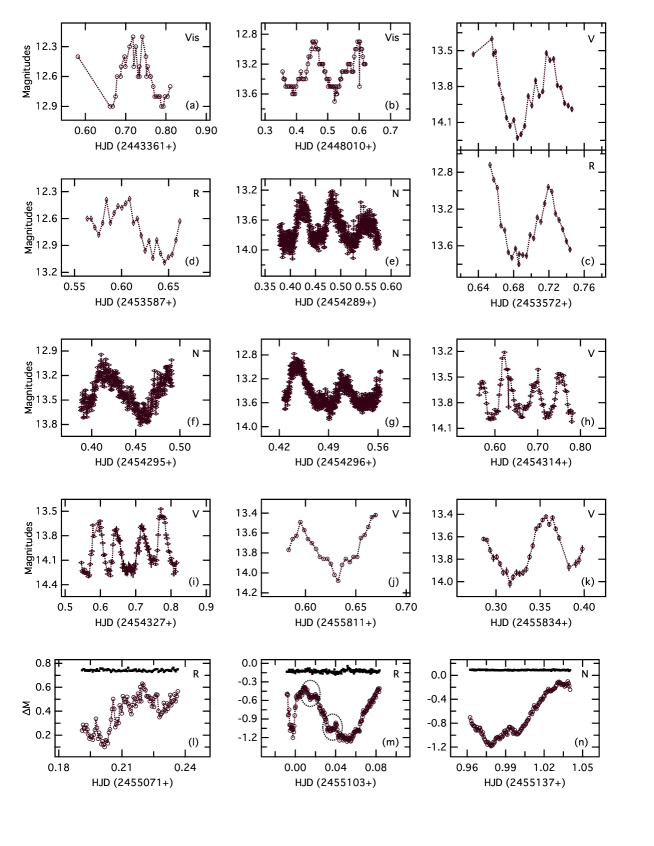
Figure 1: Fifteen high-state light curves of the polar AM Herculis spanning 1977 to 2011. The light curves in the normal, failed, and faint high states are marked by the open circles, vertical diamonds, and horizontal diamonds, respectively. The photometric filter used is given in the top right of each plot. N and V refer to white light and visual observations, respectively.

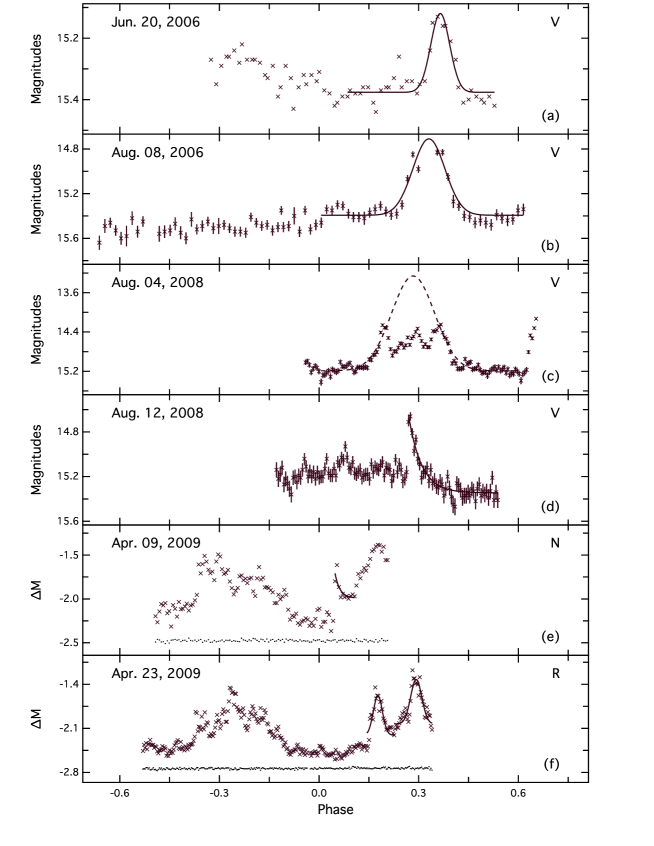
Figure 2: Six low-state light curves with seven transient events are shown in time order from top to bottom. The solid lines denote the best-fitting curves for the really complete events. The dashed line in plot (c) denotes an assumed ”disrupted” huge V-band flare event.

Figure 3: Parameter searches for e, $P_{3}$ and $\gamma$ are displayed from top to bottom. The search ranges for the three parameters are $0\sim 0.93$, $4831\sim 5831$ days, and $-1\sim 1(\times 10^{-10})$, respectively.

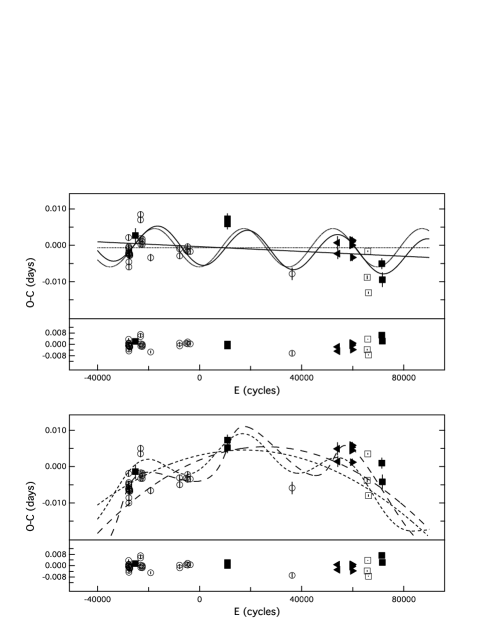
Figure 4: Upper panel shows the constant-plus-sinusoidal and linear-plus-sinusoidal fitting curves, while the lower panel shows the quadratic-plus-sinusoidal and quadratic-plus-LITE curves. Open circles, open squares, solid squares, and leftward and rightward solid triangles refer to the normal high-state data from the literature, our own photometry, the AAVSO data, and the data in the failed and faint high states, respectively.

Figure 5: Masses and separations of the third component in AM Herculis depending on its different orbital inclination are plotted with solid and dashed lines, corresponding to the left and right vertical axes, respectively.

Table 1: Details of the Photometry.

No.	Date	UTstart	Telescope	Instrument	Filter	ET	Durations
			m	CCD		s
1.	2009 Apr 09	18:10	1.0	Andor DW436 2K	N	60	0.70
2.	2009 Apr 23	19:19	0.6	Andor DW436 2K	R	25	0.92
3.	2009 Aug 27	16:33	0.85	PI MicroMAX 1024 BFT	R	30	0.36
4.	2009 Sep 28	11:47	0.6	Andor DW436 2K	R	30	0.71
5.	2009 Nov 02	11:06	1.0	Andor DW436 2K	N	40	0.61

Table 2: Minimum Light Timings for the Polar AM Herculis.

JD.Hel.	errors	type	method	wavelength	E (cycle)	$(O-C)^{\rm d}$	Ref.
2400000+
43014.712660		pri	pe	V	-27835	-.00215	(1)
43014.841268		pri	pe	V	-27834	-.00246	(1)
43015.745535		pri	pe	V	-27827	-.00069	(1)
43015.877313		pri	pe	V	-27826	+.00216	(1)
43026.4452		pri	pe	V	-27744	-.00197	(2,3)
43028.3807	.0003	pri	pe	V&R	-27729	-.00038	(2,11)
43031.728621		pri	pe	V	-27703	-.00457	(1)
43031.860554		pri	pe	V	-27702	-.00156	(1)
43032.6347		pri	pe	y&I	-27696	-.00098	(4)
43033.6610		pri	pe	I	-27688	-.00609	(4)
43062.5441		pri	pe	I&FI	-27464	-.00267	(4)
43062.802404		pri	pe	V	-27462	-.00222	(1)
43069.6354		pri	pe	I	-27409	-.00237	(4)
43083.5591		pri	pe	I	-27301	-.00280	(4)
43361.789	.002	pri	Vis	Vis	-25143	+.00264	(5)
43616.81305		pri	pe	V	-23165	+.00852	(3,6)
43616.94045		pri	pe	V	-23164	+.00699	(3,6)
43635.88762	.00060	pri	pe	690-740nm	-23017	+.00187	(7)
43636.78853	.00060	pri	pe	820-870nm	-23010	+.00029	(7)
43704.73386	.00060	pri	pe	800-835nm	-22483	+.00102	(7)
43704.86349	.00060	pri	pe	800-835nm	-22482	+.00172	(7)
43705.89342	.00059	pri	pe	750-780nm	-22474	+.00023	(7)
44133.0254	.0010	pri	pe	V	-19161	-.00339	(8,9)
45591.32259		pri	pe	V	-7850	-.00104	(3)
45600.34559		pri	pe	V	-7780	-.00294	(3)
45928.46670		pri	pe	V	-5235	-.00140	(3)
46000.27880		pri	pe	V	-4678	-.00171	(3)
46001.31151		pri	pe	V	-4670	-.00042	(3)
46132.55800		pri	pe	V	-3652	-.00175	(3)
48010.3894	.0015	pri	Vis	Vis	10913	+.00590	(5)
48010.5197	.0015	pri	Vis	Vis	10914	+.00728	(5)
51277.5182	.0017	pri	ccd	Unknown	36254	-.00788	(10)
53572.6876	.0018	pri	ccd	V&R	54056	+.00067	(5)
53587.6402	.0015	pri	ccd	R	54172	-.00231	(5)
54289.3938	.0001	pri	ccd	N/A	59615	+.00092	(5)
54289.5218	.0001	pri	ccd	N/A	59616	-.00005	(5)
54295.4540	.0001	pri	ccd	N/A	59662	+.00151	(5)
54296.4839	.0001	pri	ccd	N/A	59670	+.00008	(5)
54314.664	.001	pri	ccd	V	59811	+.00137	(5)
54327.681	.001	pri	ccd	V	59912	-.00336	(5)
55071.1983	.0005	pri	ccd	R	65679	-.00878	(11)
55103.0485	.0002	pri	ccd	R	65926	-.00161	(11)
55137.9796	.0003	pri	ccd	N	66197	-.01308	(11)
55811.6306	.0015	pri	ccd	V	71422	-.00506	(5)
55834.317	.002	pri	ccd	V	71598	-.00947	(5)

Note. —

Note. —

References. — (1) Szkody & Brownlee (1977); (2) Bailey et al. (1977); (3) Mazeh et al. (1986); (4) Olson (1977); (5)the AAVSO; (6) Szkody et al. (1980); (7) Young & Schneider (1979); (8) Bailey & Axon (1981); (9) Young et al. (1981); (10) Safar & Zejda (2002); (11) This paper.

Table 3: Least-squares Fittings for the O-C Diagram of AM Herculis.

Linear fitting	$\alpha=-1.34(\pm 0.10)\times 10^{-3}$	$\chi^{2}_{\rm\zeta}=70.8$
$O-C=\alpha+\beta E$	$\beta=9.68(\pm 0.17)\times 10^{-8}$	$\zeta=43$
		$\sigma=0^{\rm d}.0043$
Constant-plus-sinusoidal fitting	$\alpha=-6.80(\pm 2.30)\times 10^{-4}$	$\chi^{2}_{\rm\zeta}=39.1$
$O-C=\alpha+\kappa\sin[\omega E+\varphi]$	$\kappa=5.28(\pm 0.16)\times 10^{-3}$	$\zeta=41$
	$\omega=1.80(\pm 0.01)\times 10^{-4}$	$\sigma=0^{\rm d}.0034$
	$\varphi=4.74(\pm 0.03)$	$\lambda_{\rm F-test}=12.98$
		Significant level: 100%
Linear-plus-sinusoidal fitting	$\alpha=-3.80(\pm 2.50)\times 10^{-4}$
$O-C=\alpha+\beta E+\kappa\sin[\omega E+\varphi]$	$\beta=-3.31(\pm 0.79)\times 10^{-8}$	$\chi^{2}_{\rm\zeta}=39.0$
	$\kappa=5.12(\pm 0.14)\times 10^{-3}$	$\zeta=40$
	$\omega=1.78(\pm 0.02)\times 10^{-4}$	$\sigma=0^{\rm d}.0034$
	$\varphi=4.48(\pm 0.06)$	$\lambda_{\rm F-test}=8.57$
		Significant level: 99.98%
Quadratic-plus-sinusoidal fitting	$\alpha=3.12(\pm 0.52)\times 10^{-3}$
$O-C=\alpha+\beta E+\gamma E^{2}+\kappa\sin[\omega E+\varphi]$	$\beta=1.60(\pm 0.19)\times 10^{-7}$
	$\gamma=-4.56(\pm 0.64)\times 10^{-12}$	$\chi^{2}_{\rm\zeta}=37.5$
	$\kappa=4.52(\pm 0.38)\times 10^{-3}$	$\zeta=39$
	$\omega=1.56(\pm 0.04)\times 10^{-4}$	$\sigma=0^{\rm d}.0032$
	$\varphi=5.22(\pm 0.07)$	$\lambda_{\rm F-test}=8.38$
		Significant level: 99.99%
Quadratic-plus-LITE fitting	$\alpha=1.80(\pm 0.73)\times 10^{-3}$
$O-C=\alpha+\beta E+\gamma E^{2}+\tau_{\rm LITE}$	$\beta=2.84(\pm 0.30)\times 10^{-7}$
	$\gamma=-5.51(\pm 0.84)\times 10^{-12}$
	$\kappa=5.98(\pm 2.49)\times 10^{-3}$
	$P_{3}=5374^{\rm d}.04(\pm 68.07)$	$\chi^{2}_{\rm\zeta}=37.6$
	$e=0.47(\pm 0.21)$	$\zeta=37$
	$\Omega=0.28(\pm 0.55)$	$\sigma=0^{\rm d}.0033$
	$T_{0}=2448087.4(\pm 300.0)$	$\lambda_{\rm F-test}=1.96$
		Significant level: 90.39%

Figure 6: Required energy for driving the observed cyclical oscillation in the O-C diagram of AM Herculis, corresponding to different shell masses in the secondary star, are plotted as a solid line. The dotted line refers to the total radiant energy of a M5-type red dwarf over the whole oscillation period of $\sim$ 12.5 yr.

Table 4: Parameters of Low-state transient Events.

No.	Date	$F_{\rm 0}$	A	$p_{\rm 0}$	$\Gamma$	$\tau_{\rm flare}$	$\Psi$
		mag	mag	phase	phase	phase	min
1.	2006 Jun 20	15.376(7)	0.26(2)	0.365(3)	0.040(4)	-	32(3)
2.	2006 Aug 08	15.393(9)	0.68(3)	0.331(2)	0.069(3)	-	54(3)
3.	2008 Aug 04	15.189(9)	1.93(7)	0.2833(5)	0.092(2)	-	72(2)
4.	2008 Aug 12	15.35(1)	0.70(3)	0.269	-	0.039(4)	13(1)
5.	2009 Apr 09	-1.99(6)	0.28(8)	0.048	-	0.015(11)	3(2)
6.	2009 Apr 23	-2.21(6)	0.63(7)	0.177(1)	0.019(3)	-	15(2)
7.	2009 Apr 23	-2.03(4)	0.71(5)	0.293(1)	0.024(3)	-	19(2)

References

- Applegate (1992) Applegate, J. H. 1992, ApJ, 385, 621
- Araujo-Betancor et al. (2005) Araujo-Betancor, S., Gänsicke, B. T., & Long, K. S., et al. 2005, ApJ, 622, 589
- Bailey & Axon (1981) Bailey, J., & Axon, D. J. 1981, MNRAS, 194, 187
- Bailey et al. (1991) Bailey, J., Ferrario, L., & Wickramasinghe, D. T. 1991, MNRAS, 251, 37
- Bailey et al. (1988) Bailey, J., Hough, J. H., & Wickramasinghe, D. T. 1988, MNRAS, 233, 395
- Bailey et al. (1977) Bailey, J. A., Mason, K. O., & Parkes, G. E. 1977, MNRAS, 180, 35
- Beuermann et al. (2011) Beuermann, K., et al. 2011, A&A, 526, 53
- Bonnet-Bidaud et al. (2000) Bonnet-Bidaud, J. M., et al. 2000, A&A, 354, 1003
- Campbell (1985) Campbell, C. G. 1985, MNRAS, 215, 509
- Campbell et al. (2008) Campbell, R. K., Harrison, T. E., & Kafka, S. 2008, ApJ, 683, 409
- Cox (2000) Cox, A. N. 2000, Allen’s Astrophysical Quantities (4th ed.; New York; Springer)
- Crosa et al. (1981) Crosa, L., Szkody, P., Stokes, G., Swank, J., & Wallerstein, G. 1981, ApJ, 247, 984
- Cumming (2002) Cumming, A. 2002, MNRAS, 333, 589
- Dai & Qian (2010a) Dai, Z. B., & Qian, S. B. 2010a, PASJ, 62, 965
- Dai & Qian (2010b) Dai, Z. B., & Qian, S. B. 2010b, New Astronomy, 15, 380
- Dai et al. (2010) Dai, Z. B., Qian, S. B., Fernández Lajús, E., & Baume, G. L. 2010, MNRAS, 409, 1195
- Devor et al. (2008) Devor, J., et al. 2008, ApJ, 687, 1253
- Gänsicke et al. (1995) Gänsicke, B. T., Beuermann, K., & de Martino, D. 1995, A&A, 303, 127
- Gänsicke et al. (2001) Gänsicke, B. T., Fischer, A., Silvotti, R., & de Martino, D. 2001, A&A, 372, 557
- Gänsicke et al. (2006) Gänsicke, B. T., Long, K. S., Barstow, M. A., & Hubeny, I. 2006, ApJ, 639, 1039
- Goździewski et al. (2012) Goździewski, K., et al. 2012, MNRAS, 425, 930
- Hall (1989) Hall, D. S. 1989, SSRv, 50, 219
- Hearn & Richardson (1977) Hearn, D. R., & Richardson, J. A. 1977, ApJ, 213, L115
- Heise & Verbunt (1988) Heise, J., & Verbunt, F. 1988, A&A, 189, 112
- Henden & Honeycutt (1995) Henden, A. A., & Honeycutt, R. K. 1995, PASP, 107, 324
- Hessman et al. (2000) Hessman, F. V., Gänsicke, B. T., & Mattei, J. A. 2000, A&A, 361, 952
- Howell et al. (2001) Howell, S. B., Nelson, L. A., & Rappaport, S. 2001, ApJ, 550, 897
- Howell et al. (2006b) Howell, S. B., Walter, F. M., Harrison, T. E., & Huber, M. E. 2006b, ApJ, 652, 709
- Hutchings et al. (2002) Hutchings, J. B., Fullerton, A. W., Cowley, A. P., & Schmidtke, P. C. 2002, AJ, 123, 2841
- Irwin (1952) Irwin, J. B. 1952, ApJ, 116, 211
- Kafka & Hoard (2009) Kafka, S., & Hoard, D. W. 2009, PASP, 121, 1352
- Kafka et al. (2005a) Kafka, S., Honeycutt, R. K., Howell, S. B., & Harrison, T. E. 2005a, AJ, 130, 2852
- Kafka et al. (2007) Kafka, S., Howell, S. B., Honeycutt, R. K., & Robertson, J. W. 2007, AJ, 133, 1645
- Kafka et al. (2005b) Kafka, S., Robertson, J., Honeycutt, R. K., & Howell, S. B. 2005b, AJ, 129, 2411
- Kalomeni & Yakut (2008) Kalomeni, B., & Yakut, K. 2008, AJ, 136, 2367
- Knigge et al. (2012) Knigge, C. K., Baraffe, I., & Patterson, J. 2012, ApJS, 194, 28
- Kolb & Ritter (1992) Kolb, U., & Ritter, H. 1992, A&A, 254, 213
- Kozhevnikova et al. (2006) Kozhevnikova, A. V., Alekseev, I. Y., Heckert, P. A., & Kozhevnikov, V. P. 2006, IBVS, 5723, 1
- Kozhevnikova et al. (2004) Kozhevnikova, A. V., Kozhevnikov, V. P., Zakharova, P. E., Polushina, T. S., & Svechnikov, M. A. 2004, ARep, 48, 751
- Lanza (2005) Lanza, A. F. 2005, MNRAS, 364, 238
- Lanza (2006) Lanza, A. F. 2006, MNRAS, 369, 1779
- Lanza (1999) Lanza, A. F., & Rodonò, M. 1999, A&A, 349, 887
- Li et al. (1994) Li, J., Wu, K., & Wickramasinghe, D. T. 1994, MNRAS, 268. 61
- Litchfield & King (1990) Litchfield, S. J., & King, A. R. 1990, MNRAS, 247, 200
- Livio & Pringle (1994) Livio, M., & Pringle, J. E. 1994, ApJ, 427, 956
- Mason et al. (2008) Mason, E., Howell, S. B., Barman, T., Szkody, P., & Wickramasinghe, D. 2008, A&A, 490, 279
- Mayer (1990) Mayer, P. 1990, BAICz, 41, 231
- Mazeh et al. (1986) Mazeh, T., Kieboom, K., & Heise, J. 1986, MNRAS, 221, 513
- Mochnacki (1984) Mochnacki, S. W. 1984, ApJS, 55, 551
- Morales et al. (2010) Morales, J. C., Gallardo, J., Ribas, I., Jordi, C., Baraffe, I., & Chabrier, G. 2010, ApJ, 718, 502
- Nelder & Mead (1965) Nelder, J. A., & Mead, R. 1965, Computer Journal, 7, 308
- Nelson & Caton (2007) Nelson, T. E., & Caton, D. B. 2007, IBVS, 5789, 1
- Olson (1977) Olson, E. C. 1977, ApJ, 215, 166
- Paczyński (1971) Paczyński, B. 1971, ARA&A, 9, 183
- Paczyński & Sienkiewicz (1983) Paczyński, B., & Sienkiewicz, R. 1983, ApJ, 268, 825
- Pandel & Córdova (2002) Pandel, D., & Córdova, F. A. 2002, MNRAS, 336, 1049
- Pandel & Córdova (2005) Pandel, D., & Córdova, F. A. 2005, ApJ, 620, 416
- Potter et al. (2011) Potter, S. B., et al. 2011, MNRAS, 416, 2202
- Priedhorsky & Krzeminski (1978) Priedhorsky, W. C., & Krzeminski, W. 1978, ApJ, 219, 597
- Priedhorsky et al. (1978a) Priedhorsky, W. C., Krzeminski, W., & Tapia, S. 1978a, ApJ, 229, 542
- Priedhorsky et al. (1978b) Priedhorsky, W. C., Matthews, K., Neugebauer, G., Werner, M., & Krzeminski, W. 1978b, ApJ, 226, 397
- Pringle (1975) Pringle, J. E. 1975, MNRAS, 170, 633
- Qian et al. (2010) Qian, S.-B., Liao, W.-P., Zhu, L.-Y., & Dai, Z.-B. 2010, ApJ, 708, L66
- Qian et al. (2011) Qian, S.-B., et al. 2011, MNRAS, 414, L16
- Qian et al. (2012) Qian, S.-B., et al. 2012, MNRAS, 423, 3646
- Ramsay et al. (2004) Ramsay, G., Cropper, M., Wu, K., Mason, K. O., Córdova, F. A., & Priedhorsky, W. 2004, MNRAS, 350 1373
- Rappaport et al. (1983) Rappaport, S., Verbunt, F., & Joss, P. C. 1983, ApJ, 275, 713
- Robinson et al. (1981) Robinson, E. L., Barker, E. S., Cochran, A. L., Cochran, W. D., & Nather, R. E. 1981, ApJ, 251, 611
- Safar & Zejda (2002) Safar, J., & Zejda, M. 2002, IBVS, 5263, 1
- Schmidt et al. (1983) Schmidt, G. D., Stockman, H. S., & Grandi, S. A. 1983, ApJ, 271, 735
- Schwope et al. (1993) Schwope, A. D., Beuermann, K., Jordan, S., & Thomas, H.-C. 1993, A&A, 278, 487
- Schwope et al. (2001) Schwope, A. D., Schwarz, R., Sirk, M., & Howell, S. B. 2001, A&A, 375, 419
- Shafter et al. (1985) Shafter, A., Szkody, P., Liebert, J., Penning, W. R., Bond, H. E., & Grauer, A. D. 1985, ApJ, 290, 707
- Shakhovskoy et al. (1993) Shakhovskoy, N. M., Alexeev, I. Y., Andronov, I. L., & Kolesnikov, S. V. 1993, Ann. Israeli Phys. Soc., 10, 237
- Shao & Li (2012) Shao, Y., & Li, X.-D. 2012, ApJ, 745, 165
- Soberman et al. (1997) Soberman, G. E., Phinney, E. S., & van den Heuvel, E. P. J. 1997, A&A, 327, 620
- Southwell et al. (1995) Southwell, K. A., Still, M. D., Connon, S. R., & Martin, J. S. 1995, A&A, 302, 90
- Spruit & Ritter (1983) Spruit, H. C., & Ritter, H. 1983, A&A, 124, 267
- Stehle et al. (1996) Stehle, R., Ritter, H., & Kolb, U. 1996, MNRAS, 279, 581
- Szkody & Brownlee (1977) Szkody, P., & Brownlee, D. E. 1977, ApJ, 212, L113
- Szkody et al. (1980) Szkody, P., Cordova, F. A., Tuohy, I. R., Stockman, H. S., Angel, J. R. P., & Wisniewski, W. 1980, ApJ, 241, 1070
- Tapia (1977) Tapia, S. 1977, ApJ, 212, L125
- Terada et al. (2010) Terada, Y., Ishida, M., Bamba, A., Mukai, K., Hayashi, T., & Harayama, A. 2010, ApJ, 721, 1908
- Torres et al. (2010) Torres, G., Andersen, J., & Giménez, A. 2010, A&AR, 18, 67
- Townsley & Bildsten (2003) Townsley, D. M., & Bildsten, L. 2003, ApJ, 596, L227
- Vida et al. (2009) Vida, K., Oláh, K., Kövári, Z., Korhonen, H., Bartus, J., Hurta, Zs., & Posztobányi, K. 2009, A&A, 504, 1021
- Warner (1995) Warner, B. 1995, Cataclysmic Variable Stars (1st ed.; Cambridge: Cambridge Univ. Press)
- Webbink & Wickramasinghe (2002) Webbink, R. F., & Wickramasinghe, D. T. 2002, MNRAS, 335, 1
- Wickramasinghe & Martin (1985) Wickramasinghe, D. T., & Martin, B. 1985, MNRAS, 212, 353
- Wickramasinghe & Wu (1994) Wickramasinghe, D. T., & Wu, K. 1994, MNRAS, 266 L1
- Wu & Kiss (2008) Wu, K., & Kiss, L. L. 2008, A&A, 433, 439
- Young & Schneider (1979) Young, P., & Schneider, D. P. 1979, ApJ, 230, 502
- Young et al. (1981) Young, P., Schneider, D. P., & Shectman, S. A. 1981, ApJ, 245, 1043
- Zeilik et al. (1982) Zeilik, M., Elston, R., & Henson, G. 1982, IBVS, 2200, 1
- Zhang et al. (2010) Zhang, L.-Y., Zhang, X.-L., & Zhu, Z.-Z. 2010, New Astronomy, 15, 362