Kelvin-Helmholtz instability of a coronal streamer

Abstract

The shear-flow-driven instability can play an important role in energy transfer processes in coronal plasma. We present for the first time the observation of a kink-like oscillation of a streamer probably caused by the streaming kink-mode Kelvin-Helmholtz instability. The wave-like behavior of the streamer was observed by Large Angle and Spectrometric Coronagraph Experiment (LASCO) C2 and C3 aboard SOlar and Heliospheric Observatory (SOHO). The observed wave had a period of about 70 to 80 minutes, and its wavelength increased from $2\;R_{\odot}$ to $3\;R_{\odot}$ in about 1.5 hours. The phase speeds of its crests and troughs decreased from $406\pm 20$ to $356\pm 31\mathrm{kms^{-1}}$ during the event. Within the same heliocentric range, the wave amplitude also appeared to increase with time. We attribute the phenomena to the MHD Kelvin-Helmholtz instability which occur at a neutral sheet in a fluid wake. The free energy driving the instability is supplied by the sheared flow and sheared magnetic field across the streamer plane. The plasma properties of the local environment of the streamer were estimated from the phase speed and instability threshold criteria.

1 Introduction

The Kelvin-Helmholtz instability (KHI) driven by a shear of the flow velocity, has been observed in various astrophysical environments. In the solar atmosphere, Berger et al. (2010) and Ryutova et al. (2010) discovered it in a prominence from Hinode Solar Optical Telescope observations. Foullon et al. (2011) and Möstl et al. (2013) found that it could develop at the flank of a fast coronal mass ejection. Ofman & Thompson (2011) identified a vortex-shaped feature caused by the KHI on the boundary of a dimming area during the eruption of an active region. It has been shown by Chandrasekhar (1961) that the presence of a magnetic field tangential to the boundary surface and directed along the flow stabilizes the hydrodynamic KHI. For a symmetric shear layer, the instability can only grow if the the velocity jump across the boundary between the two uniform regions exceeds twice the Alfvén velocity on either side.

The instability growth is modified when the field and density profiles across the boundary are asymmetric or if the shear layer has a finite width. Instability calculations and simulations have been performed to model the magnetospheric current sheet, astrophysical jets and streamer sheets in the solar corona. The model adopted for these cases were 2D and 3D force-free or pressure balanced current sheets with a jet or a wake layer centered at the current sheet (Lee et al., 1988; Wang et al., 1988; Dahlburg et al., 1998; Einaudi, 1999; Dahlburg et al., 2001; Zaliznyak et al., 2003). Owing to Galilean invariance, the wake, a layer of reduced speed embedded in a uniform background flow, is equivalent to the jet case for otherwise identical plasma parameters and produces the same instability growth rates but shifted phase speeds (Einaudi et al., 1999). More recently, 2.5 D and 3 D simulations were performed to shed more light on the velocity and magnetic shear driven instabilities in the nonlinear regimes (Bettarini et al., 2006, 2009).

From all these studies, three different modes could be distinguished during the initial phase of the instability. For low Alfvénic Mach numbers below about two, the instability is strongly influenced by the magnetic field and shows plasmoid formation as a result of the tearing mode instability (or resistive varicose mode) (e.g., Einaudi et al., 1999). For Alfvénic Mach numbers above about two, the hydrodynamic behavior overwhelms the magnetohydrodynamic evolution. A symmetric and an asymmetric oscillatory mode evolve in such a situation termed kink (or sinuous) mode and sausage (or ideal varicose) mode.

Using the linear theory, Lee et al. (1988) derived analytical expressions for the growth rates and phase speeds of the three modes of a jet assuming a four layer model each with constant plasma parameters. They found that the kink mode dominates over the sausage mode when the value of $\beta$ (ratio of thermal to magnetic pressure) in the ambient plasma exceeds unity. This value of $\beta$ is, however, linked to other equilibrium parameters of the current sheet by the requirement to maintain the net pressure balance, e.g., the ratio of the density between the current sheet and its ambient plasma. In an accompanying paper, Wang et al. (1988) applied the wake model to the heliospheric current sheet and considered the influence of difference between the width of the velocity shear layer and the width of the current sheet on the growth rate. Numerical simulations of the current carrying wake with various plasma parameters suggest that the kink mode often dominates for the large $\beta$ parameters considered, except for long wavelengths of the perturbations (Dahlburg et al., 1998, 2001; Zaliznyak et al., 2003). Even though the instability growth rate decreases steadily with increasing sonic Mach number, i.e., with decreasing $\beta$, the simulations do not show a drastic threshold for $\beta$ or for the sonic Mach number like is exists for the Alfvénic Mach number.

The quasi 2D current plane at the tip of a helmet streamer seems to become particularly close to the model geometry adopted in the above simulations. However, contrary to the ease with which the kink mode is excited in the simulations, it is not observed as frequently. Indeed, SOHO/LASCO observations show the almost continuous ejection of plasmoids from the tip of helmet streamers, (e.g., Sheeley et al., 1997). They were interpreted as the development of the tearing-type reconnection to a nonlinear varicose (sausage-like) fluid instability discussed above (Einaudi et al., 1999, 2001). On the other hand, the equivalent kink-like instability along a streamer has to the knowledge of the authors not been observed.

In this paper we report the rare observation of kink-like oscillations in the current sheet of a coronal streamer. On June 3, 2011 a narrow streamer was emerging from behind the occulter of SOHO/LASCO C2 and C3 which after about 7:30 exhibited a clear oscillating behavior.

A wave-like motion of a streamer was also observed by Chen et al. (2010) which the authors claim to have been excited by the eruption of a fast coronal mass ejection (CME) nearby. In their observations, the wave was excited impulsively and steadily decayed afterwards. In the case of the streamer on June 3 reported here, no CME occurred close to the streamer, neither in time nor in space. Also, the wave amplitude in this event stayed constant for hours or even slightly increased with time. We therefore attribute this oscillation to an instability rather than to an impulsive excitation. To our knowledge it is the first observation of a streamer wave which was probably caused by the streaming kink instability. In Section 2, the observations of the streamer wave by the LASCO coronagraph and the retrieving of the wave shape are described. In Section 3, we compare the potential of the streaming kink instability and other competing MHD modes of the KHI as a source for this wave. In the last section, the obtained results will be summarized and discussed.

2 Observations and data reduction

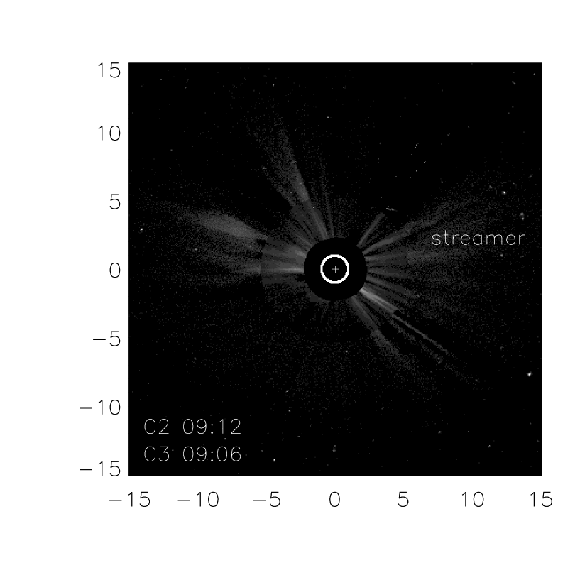
Figure 1: The oscillating streamer observed by C2 at 09:12 UT and observed by C3 at 09:06 UT. The white circle indicates the solar limb, and the plus sign represents the Sun center. A movie showing the evolution of the oscillating steamer is available online. The units are in solar radius.

The oscillating feature was observed by the LASCO (Brueckner et al., 1995) C2 and C3 coronagraphs aboard SOHO. LASCO C2 has a FOV from 2 to 6 R_⊙, C3 from 3.7 to $30\;R_{\odot}$. The wave-like motion of the streamer first appeared in the C2 field of view at a distance 3 to $4\;R_{\odot}$ at 05:48 UT on June 3, 2011. The wave which developed then propagated almost radially to a distance of about $11\;R_{\odot}$ at 10:30 UT. At larger distances, the phenomenon becomes impossible to observe due to the low signal to noise. A movie showing the streamer wave can be found in the online material. The end of the wave-like motion was accompanied by a disruptive eruption beginning around 13:25 UT. In Figure 1, a snapshot of the oscillation is presented. The streamer with the wave-like feature is located in the first quadrant of the image plane and is rooted at a latitude around 27.5^∘.

From the LASCO images, the streaming feature appears as a white-light jet (Wang et al., 1998; Feng et al., 2012). Usually, a jet can be traced down to its footpoints at the solar surface. However, AIA/SDO did not observe any possible source for the jet at lower altitude. Moreover, an elongated structure existed at the same position for many hours before the appearance of the wave. An alternative possibility is the leakage of plasma from the cusped magnetic field lines above a helmet streamer. The cusp is a hot region at the streamer top with low magnetic field strength and the magnetic boundary concavely bent outwards. In this region the plasma $\beta$ may easily have values above unity. Thus the magnetic field confinement can be considered marginal and the streamer plasma may occasionally leak out of the cusp region to feed the slow solar wind. It is generally observed that the cusp altitude is below 2 to $2.5\;R_{\odot}$, very close to the inner boundary of the LASCO C2 FOV (Chen et al., 2010). In EUV observations, due to the relatively low density of the helmet streamer plasma and the restricted field of view, it is usually difficult to see the dome part of a streamer. For that reason, AIA was probably not able to see the lower helmet counterpart associated with the observed streamer.

To clarify the spatial context of this event, we show an EUV image observed at $\lambda=28.4$ nm by the ahead spacecraft of Solar TErrestrial RElations Observatory (STEREO, Kaiser et al., 2008) in the upper panel of Figure 2. At the time of observation, STEREO A was located about 90 degrees west of the Sun-Earth line and looks almost vertically down onto the longitude of the streamer. Two coronal holes, one above and one below the streamer latitude are indicated.

The lower panel of Figure 2 shows the field lines from a PFSS model emerging from a $20^{\circ}$ wide longitude range around the limb and from latitudes of $27.5\pm 30^{\circ}$. The field extrapolation was produced from a synodic magnetogram observed by the Helioseismic and Magnetic Imager (HMI; Schou et al., 2012) aboard Solar Dynamic Observatory (SDO) for Carrington rotation (CR) 2110. In this magnetogram, the limb longitude is intersected by two neutral lines which for a source surface height $r_{SS}<1.6R_{\odot}$ results in two current sheets above the limb. The southern sheet matches very closely the latitude of observed oscillating streamer. For larger $r_{SS}$, the two current sheets merge and the PFSS field beyond the source surface height becomes unipolar. In this case, the observed streamer would have to be interpreted as a pseudostreamer Wang et al. (2007). From the observations in Fig. 1, we can state that the source surface height $r_{SS}$ for the oscillating streamer must be well less than the LASCO C2 occulter radius of about 2.2 $R_{\odot}$. The fact that a value of $r_{SS}<1.6R_{\odot}$ produces a current sheet within a few degrees of the observed streamer latitude gives us confidence that the observed streamer is associated with a current sheet and the streamer bulge is confined to low altitudes.

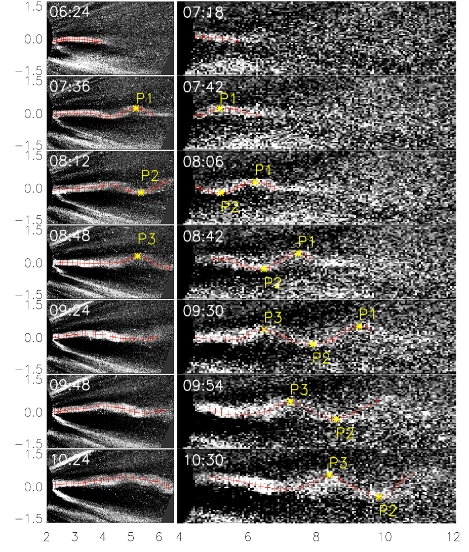
Figure 3: Some selection of the traced streamer in C2 and C3 images. The streamer was rotated clockwise by $27.5^{\circ}$ to be horizontally located. The traced streamer at different instances is delineated by red plus signs. The first crest is indicated by P1, the first trough by P2, and the second crest by P3. For the context of the streamer, a strip from $-1.5\;R_{\odot}$ to $1.5\;R_{\odot}$ in north-south direction, from $2\;R_{\odot}$ to $6.5\;R_{\odot}$ in east-west direction was cropped in C2 images. In C3 images, the range in the east-west direction is from $4\;R_{\odot}$ to $12\;R_{\odot}$.

In Figure 3, some selected image frames which zoom into the streamer wave are presented. To make the streamer structure more prominent, a pre-event image immediately before the streamer’s appearance was subtracted from the following sequence of C2 and C3 images, respectively. For a better visualization of the wave-like structure and its propagation, the streamer was rotated clockwise by 27.5^∘ to horizontal. The shape of the streamer axis was traced by hand and marked by red plus signs. In each frame, if applicable, the crest and trough are indicated in yellow. The first crest is enumerated by P1, the first trough by P2, and the second crest by P3. From the C2 observations, the streamer started to oscillate only above the distance of about $3\;R_{\odot}$ from the Sun center. After 08:12 UT, the streamer brightness intensified, which can be seen, e.g., from the large brightness gradient along the streamer near $4.6\;R_{\odot}$ at 09:24 UT. This also modified the shape of the streamer especially below the heliocentric distance of 5 to $6\;R_{\odot}$.

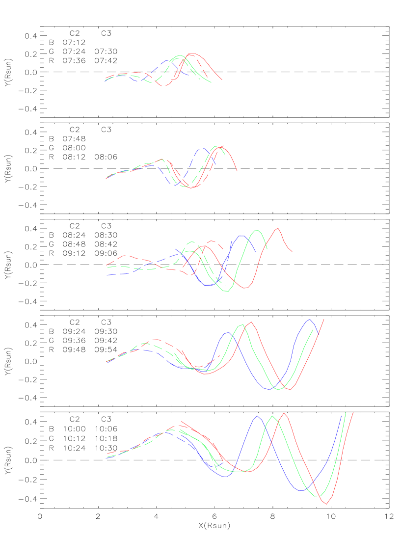
Figure 4: The traced streamer in all the frames observed from 07:12 UT to 10:30 UT by C2 and C3. The streamer within C2 FOV is indicated by long dashed lines, and within C3 FOV by solid lines. The streamer traced at different times are shown in red (R), green (G), and blue (B) color. Those with observational time by C2 and C3 within 6 minutes are displayed with the same color.

A complete dataset of the traced streamer axis from C2 and C3 images is displayed in Figure 4. The time cadences of the C2 and C3 images were both 12 minutes in general but occasionally had an observational gap of more than 12 minutes. The streamer traced in C2 is delineated with dashed lines, in C3 with solid lines. Streamer traces observed with a time difference of less than 6 minutes are drawn in the same color. Although after 08:12 UT, the full length of the streamer was traced out, we will neglect in the further analysis the segment behind the brightness intensification noted above.

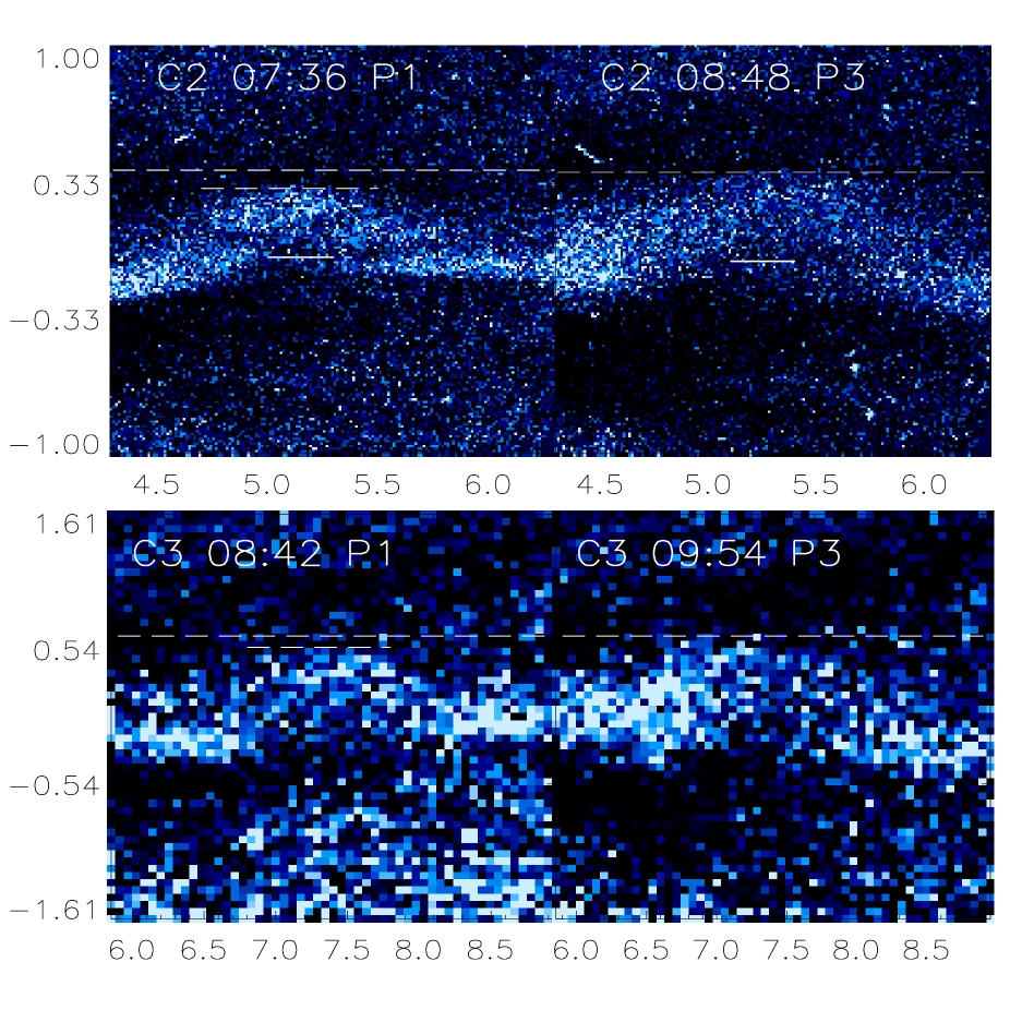
Figure 5: Segments of the streamer around the crests P1 and P3 at different heliocentric distances. Dashed lines mark the upper boundary of the crests P1 and P3, the solid bars indicate their lower boundary. The $X$ and $Y$ axes are in units of $R_{\odot}$.

The traced streamer positions in Figure 4 may be subject to some uncertainty. To investigate the amplitude variation with distance and time, the streamer segments around the first and second crests P1 and P3 are compared in Figure 5 after they propagated for somewhat more than an hour from the C2 field of view into C3. The upper dashed horizontal line in Figure 5 marks the peak of P3, the lower dashed line the peak of P1. It shows that the upper boundary of the crests P1 and P3 increased from 0.3 to $0.5\;R_{\odot}$ when they propagated to larger distances from about 5.2 to $7.5\;R_{\odot}$, which indicates the increase of their amplitudes with distance. If we use the two short solid lines as the lower boundary of the streamer segment around its peak at 07:36 UT and 08:48 UT, the amplitude, as calculated from half the average distance of the lower and upper boundaries, increases slightly from 0.14 to $0.17\;R_{\odot}$. It also increases slightly with time during our observations. Although these estimates of the amplitude increase are not very precise due to data noise, it is very unlikely that the streamer in our study experienced an amplitude decrease as it was observed by Chen et al. (2010). Therefore, we rule out that the wave-like behavior of the streamer in our observations was caused by an interaction of the streamer with a CME as reported in their paper.

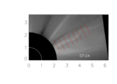
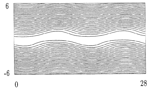
Figure 6: (Upper) A cut of the C2 image at 07:24 UT in which the streamer started to show clear oscillations. Eight short red lines mark the positions where the brightness distribution accross the streamer is measured. The $X$ and $Y$ axes are in units of $R_{\odot}$. (Lower) The magnetic field configuration of the streaming kink instability adopted from Figure 1 in Wang et al. (1988). The $X$ and $Y$ axes are in units of the half thickness of the current layer.

Since the brightness in LASCO C2 and C3 is caused by Thomson scattering of electrons in the corona, the observed coronagraph brightness is proportional to the column density along the line-of-sight. Moreover, we conclude form the fact that the streamer can distinctly be seen on the dark background sky and appears like a narrow ribbon that we observe the streamer more or less edge-on. We therefore assume that the observed column densities can serve as a proxy of the volume density along a profile normal to the streamer axis. In the upper panel of Figure 6, the eight red lines mark the profiles along which the brightness measurements were performed. Note that the pre-event image was not subtracted from this image. Instead, a monthly-minimal image was subtracted to remove the stray light and/or the F corona.

In Figure 7, we display the brightness distribution across the streamer on these eight profiles, extracted from the observation at 07:24 UT when the oscillation of the streamer started to become pronounced. Two dotted lines represent the maximum $\rho_{s}$ and the assumed background $\rho_{\infty}$ of the brightness. Obviously, the ratio $\rho_{s}/\rho_{\infty}$ declines approximately with heliocentric distance from $\rho_{s}/\rho_{\infty}\simeq 2$ to $\rho_{s}/\rho_{\infty}\simeq 1.5$ except at $r=4\;R_{\odot}$. The brightness distribution at $r=2.5\;R_{\odot}$ was contaminated by a bright structure in the south of the streamer. We therefore used for this heliocentric distance the background estimate from $r=2.8\;R_{\odot}$ instead. Interestingly, the streamer wave is discernible only at a distance beyond $r=3.5\;R_{\odot}$ when the density ratio has already settled to its lower bound of $\rho_{s}/\rho_{\infty}\simeq 1.5$. As another parameter, we can estimate from Figure 7 the width of the current sheet. For altitudes below $r=4\;R_{\odot}$ the streamer is well concentrated with a half-width of $\delta\simeq 0.2\;R_{\odot}$. Beyond $4\;R_{\odot}$ the streamer appears more diffusive probably due to decreasing signal-to-noise.

There are two major sources of uncertainties involved in the estimate of the density ratio. One is the unknown line-of-sight depth of the streamer. We assumed the density ratio to be equal the ratio of the observed column densities which implies an infinite streamer depth. If the real depth of the streamer is well less than $R_{\odot}$, we underestimate the density ratio. The other unknown is related to the background subtraction of the coronagraph image. To obtain an upper bound of the ratio, instead of the monthly-minimum background, a yearly-minimal image was utilized. The corresponding density ratios are indicated in the parentheses in each panel. Although the ratios increase slightly, the trend of decreasing ratio with distance is clear.

Based on the retrieved wave-like structure in Figure 4, we have estimated parameters which characterize the streamer wave. The heliocentric distance of the crests and troughs, P1, P2 and P3, is plotted in Figure 8 as a function of time. Applying linear fits to their space-time positions yields a phase speed for P1, P2 and P3 of $406\;\mathrm{kms^{-1}}$, $374\;\mathrm{kms^{-1}}$ and $356\;\mathrm{kms^{-1}}$, respectively. The decrease of the phase speed from P1 to P3 can be directly concluded from the slight divergence of the fit lines in Figure 8. As seen in Figure 3, at 08:06 UT the half wavelength $\overline{P1P2}$ was about $1\;R_{\odot}$; by 09:30 UT the half wavelength $\overline{P1P2}$ had enlarged to $1.5\;R_{\odot}$. The period of the wave was measured from the time interval between the first to the second crest, P1 and P3. We found about a period of 72 minutes at $r=5\;R_{\odot}$ and 84 minutes at $r=9\;R_{\odot}$.

The major uncertainty involved in the above analyses comes from the delineation of the streamer profile in the LASCO observations (Figure 3). Once the profiles are determined, tracking the crests and troughs of the profiles and fitting a linear function to their distance-time plots only contributes to a minor uncertainty. We assume that the uncertainty of the streamer identification corresponds to the half width $\delta$ of the streamer of about $\pm 0.2\;R_{\odot}$. This is also the uncertainty of the positions of the crests and troughs in Figure 8. The linear fits bearing such uncertainties produce a 1-sigma error of the three velocity estimates of 16, 9 and $24\;\mathrm{kms^{-1}}$.

3 The streaming kink instability

Analytical and MHD simulations have shown that streaming sausage, kink and tearing instabilities can occur in presence of sheared velocity and magnetic field systems. At the tip of a helmet streamer, the magnetic field has opposite directions on the two sides with a neutral sheet inside. The field strength inside the streamer is probably well below the value outside and the pressure deficit is compensated by an enhanced plasma density. The plasma velocity assumes a minimum in the neutral current sheet which can be considered the source of the slow solar wind and increases towards both sides where the dilute plasma is accelerated into the fast solar wind. Plasma blobs probably formed by the streaming sausage and tearing instabilities and convected away by the surrounding solar wind flow have been observed at the tip of the helmet streamer (e.g., Sheeley et al., 1997). So far however, kink mode waves have not been detected yet. In view of the amplitude increase of the wave-like structure we observe, we tend to believe that it is instability-driven. The increase of the perturbation is probably fed from the kinetic energy of the surrounding solar wind plasma.

A very robust threshold for the streaming kink and sausage instability found in many simulations concerns the velocity difference of the shear flow. In the simulation of Chen et al. (2009), an Alfvén speed of $20\;\mathrm{kms^{-1}}$ inside and of $75\;\mathrm{kms^{-1}}$ outside of the current sheet was assumed. With these parameters Chen et al. (2009) could excite both modes with a velocity difference for the shear flow of $100\;\mathrm{kms^{-1}}$ for the kink and about $150\;\mathrm{kms^{-1}}$ for the sausage mode.

If we take the measurements by the Ulysses space craft (McComas et al., 2008) as a typical estimate of the solar wind speed and its gradients, these threshold values for the velocity shear can be easily achieved. Note, however, that the Ulysses measurement were made beyond 1 AU where the solar wind has been accelerated to its asymptotic speed which probably has not yet been reached at 10 $\;R_{\odot}$. Also the Alfvén speed assumed by Chen et al. (2009) is relatively low. A typical value beyond $2\;R_{\odot}$ is $200\;\mathrm{kms^{-1}}$ (e.g., Warmuth and Mann, 2005). However, in cusp and streamer regions the field strength is probably reduced with respect to this average.

Lee et al. (1988) found from an analytic solution of a four-layer model that the kink mode dominates over the sausage mode when $\beta$ in the ambient plasma exceeds unity, or equivalently, $\rho_{s}/\rho_{\infty}$ is less than about 2. Their model consists of two layers of width $\delta$ with adjacent half spaces. The magnetic field is tangential to the boundaries and asymmetric to the central boundary. The flow is parallel to the magnetic field and symmetric with respect to the central boundary. Keeping the plasma temperature constant throughout, there are besides the temperature six parameters: magnetic field, flow speed and plasma density, each inside the inner layers and in the half space, which can be varied. The unperturbed pressure balance of the current sheet reduces the number of independent parameters by one.

In view of this number of model parameters, we have reexamined Lee et al.’s dispersion relation (eqs.(34) and (35) of Lee et al., 1988) in the parameter range we find most appropriate for our observations. We found above a half-width of the streamer of about $\delta\simeq 0.2\;R_{\odot}$ and a typical wave number of $k=2\pi/2.5\;R_{\odot}^{-1}$ for the wave structure which yields $k\delta=0.5$. Assuming the magnetic field in the streamer was half the outside value, the temperature was about 1 MK, and taking into account the pressure balance (equ.(10) in Lee et al., 1988)

$$\rho_{p}=\rho_{\infty}\left[\frac{T_{\infty}}{T_{p}}+\frac{V_{A\infty}^{2}}{2RT_{p}}\left(1-\frac{B_{p}^{2}}{B_{\infty}^{2}}\right)\right],$$

the observed $\rho_{s}/\rho_{\infty}=1.5$ results in $V_{A\infty}\approx 100\;\mathrm{kms^{-1}}$, and the plasma-$\beta$ then adjusts to values of 1.5 outside and 9 inside the streamer.

In Lee et al.’s (1988) work, large constant growth rates are obtained for $k\delta>2$ for the both kink and sausage mode. They are probably due to the sharp step-like gradients between the piece-wise constant model profiles assumed. Numerical simulations with more realistic profiles (e.g., Zaliznyak et al., 2003) yield maximum growth rates well below $k\delta\simeq 1$. From these dispersion relations it is found that the phase speed does not vary drastically with wave number and asymptotically in the limit $k\delta\rightarrow\infty$ becomes

$$V_{\phi}=V_{\infty}+\frac{\rho_{s}}{\rho_{s}+\rho_{\infty}}\Delta V_{s}$$

where $\rho_{\infty}$ and $V_{\infty}$ are the density and flow speed outside the streamer, $\rho_{s}$ and $V_{\infty}+\Delta V_{s}$ are the same parameters inside the streamer. Note that different from Lee et al. (1988), we here assume a wake model for the streamer so that $\Delta V_{s}$ is negative. In order to reach the observed phase velocities of $V_{\phi}\simeq 400\dots 350\;\mathrm{kms^{-1}}$, the choice of values for $V_{\infty}$ and $\Delta V_{s}$ is considerably constrained. The set of values for which we find a reasonable agreement with the observations is $V_{\infty}=500\;\mathrm{kms^{-1}}$ and $\Delta V_{s}=-150\;\mathrm{kms^{-1}}=-1.5V_{A\infty}$.

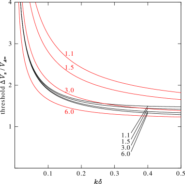
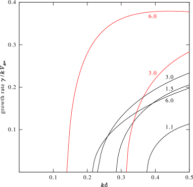
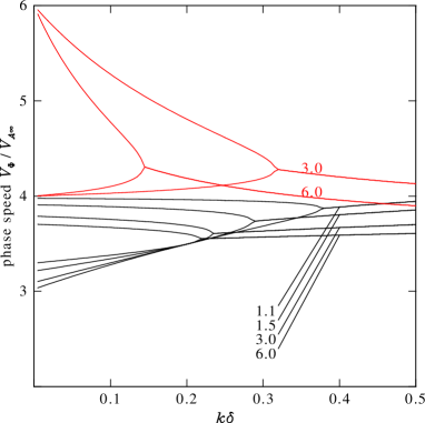
Figure 9: Normalized velocity shear threshold, growth rate and phase speed versus wave number for different density ratios $\rho_{s}/\rho_{\infty}$ from the dispersion equation for the kink(black) and sausage(red) mode of (Lee et al., 1988). The curves are labelled according to the density ratio $\rho_{s}/\rho_{\infty}$. For the ratios 1.5 and 1.1, the sausage mode is stable in the wavelength range shown. Growth rate and phase speed were calculated for $\Delta V_{s}=-1.5\;V_{A\infty}$. Other parameters are given in the text.

In Fig. 9 for different values of the density ratio $\rho_{s}/\rho_{\infty}$, we show the threshold values for $\Delta V_{s}$, growth rate and phase speed for $V_{\infty}=500\;\mathrm{kms^{-1}}$ and $\Delta V_{s}=-150\;\mathrm{kms^{-1}}$. From the threshold diagram we conclude that waves with $k\delta\simeq$ 0.3 to 0.5 can readily be excited by a velocity shear $\Delta V_{s}$ not much above $V_{A\infty}$. We have to keep in mind that the Alfvén velocity is reduced inside the streamer layer by a factor two. The adopted value of $|\Delta V_{s}|=1.5V_{A\infty}$ for the growth rate and phase speed below is just above the threshold. If the threshold is exceeded, the largest growth rates for the kink mode occur at $k\delta>0.5$ and are achieved for the density ratio $\rho_{s}/\rho_{\infty}$ between 1.5 and 3. For larger density ratios, the sausage mode grows faster. Concerning the observed density ratio about 1.5, the sausage mode is stable and has a zero growth rate. Therefore, only the kink mode was observed. For $k\delta$ much larger than 0.5, we believe that the analytical dispersion based on a model with sharp, step-like gradients overestimates the growth rate.

The phase speed of the kink mode for the observed density ratio around 1.5 and the observed wave number $k\delta\simeq 0.5$ is $V_{\phi}=3.8\;V_{A\infty}=380\;\mathrm{kms^{-1}}$. This comes again close to what we observed. Note that each unstable kink and sausage mode is a coalescence of an up- and downshifted propagating MHD boundary wave so that the phase speed splits for low wave numbers where the mode becomes stable. When unstable, the two waves merge to a pair with complex conjugate frequencies and a unique phase speed.

The growth rates rise quite steeply once the threshold is exceeded and a value of $\gamma=0.2kV_{A\inf}$ seems not unrealistic. However, we have to keep in mind that the instability occurs in an inhomogeneous environment with fixed boundary conditions on the sunward side of the streamer. At this side the wave amplitude can only have noise level. Under these conditions, the instability becomes convective instead of showing temporal growth.

The growth scale which we can expect is $V_{\phi}/\gamma=V_{\phi}/(0.2\,kV_{A\infty})$. With the parameters used in our model, $V_{\phi}=380\;\mathrm{kms^{-1}}$ and $V_{A\infty}=100\;\mathrm{kms^{-1}}$, we estimate the e-folding growth scale to $3.8/0.2\cdot\lambda/2\pi=3\lambda$. From the increase of the observed wave amplitude apparent from the streamer traces in Figure 4, this number does not seem unrealistic.

4 Conclusions and discussion

We present for the first time the observation of an oscillating streamer probably driven by the streaming kink instability, a mode of the MHD Kelvin-Helmholtz instability. The streamer presented a period of about 70 to 80 minutes, and its wavelength increased from 2 to $3\;R_{\odot}$ in about 1.5 hours. The phase speed of the oscillation varied from $406\pm 20$ to $356\pm 31\;\mathrm{kms^{-1}}$ for different crests and trough. These derived properties of the wave structure places constraints on the plasma environment in which the instability took place. We find a low Alfvén speed of about 100 $\mathrm{kms^{-1}}$ and a high flow speed of about 500 $\mathrm{kms^{-1}}$ outside the streamer. It also turns out that the flow speed within the streamer was 150 $\mathrm{kms^{-1}}$ lower.

In previous studies, oscillations of a streamer have been observed following interaction with a fast CME (Chen et al., 2010, 2011). The phenomenon was termed as a “streamer wave” by the authors. A distinct characteristic of their observation was the decrease of the oscillation amplitude with time (see their Figure 4) due to the convection of the energy with the outward propagation of the wave. In the event reported here, no CME was detected in the LASCO field of view. Also, the coronagraph observations by STEREO A and B did not show any CME activity close to the streamer. Another distinction from the previously reported oscillating streamer, within the same distance range, was the increasing amplitude of the wave with time. The streamer also displayed a pronounced increase in amplitude when it convected to larger heliocentric distances. This is evidence that the wave motion was excited by an instability.

Our assumptions are that the streamer is a 1D layer with plasma flow and magnetic field mutually parallel and normal to the layer gradient according to the model invoked by Lee et al. (1988). The plasma velocity is symmetrically distributed, the magnetic field varies asymmetrical and the plasma temperature is constant throughout. We do not distinguish between the widths of the velocity shear, the magnetic field shear, and the scale of the density variation. With these model assumptions we could reproduce many features of our observation.

In order to reproduce the observed phase speed we had to invoke a high flow speed and a low Alfvén speed outside of the streamer. Typically assumed values for slow solar wind in the distance range from 8 to $10\;R_{\odot}$ are $V_{A\infty}\simeq 200\;\mathrm{kms^{-1}}$ (Warmuth and Mann, 2005) and $V_{\infty}\simeq 200\;\mathrm{kms^{-1}}$ (e.g., Sheeley et al., 1997). The latter authors determined $V_{\infty}$ from the velocity of density fluctuations drifting off streamer tips. They also show that the speed of individual density blobs scatters enormously around the above quoted average and may reach more than $600\;\mathrm{kms^{-1}}$ in some cases. The value of $V_{\infty}=500\;\mathrm{kms^{-1}}$ which we conclude from our observations is therefore not unrealistic. Moreover, at the time of our observations, the streamer was sandwiched between two nearby coronal holes to the north and south of the streamer (see Figure 2). It does not seem impossible, that the fast solar wind from these coronal holes had some impact on the flow speed $V_{\infty}$ in the vicinity of the streamer.

In our analysis, we also had to assume a low Alfvén speed $V_{A\infty}$ to reproduce the observed phase speed of 350 to $400\;\mathrm{kms^{-1}}$. Our value $V_{A\infty}=100\;\mathrm{kms^{-1}}$ is low but still slightly higher than the value taken by Chen et al. (2009) in their simulations of a coronal streamer. Higher values for $V_{A\infty}$ require even larger flow speeds $V_{\infty}$ and also a larger velocity shear magnitude $|\Delta V_{s}|$ inside the streamer. From our estimates, $\Delta V_{s}=-1.5V_{A\infty}$ just exceeds the threshold condition. For a larger $\Delta V_{s}$ and also for density ratios $\rho_{s}/\rho_{\infty}>3$, the kink instability would be superseded by the sausage mode. We believe that these special conditions are the reason why the kink mode is only seldom observed with coronal streamers compared to the sausage mode. This alternative mode manifests itself in the formation of density fluctuations and plasmoids which are more commonly observed in coronal streamers.

The streamer is also special in that its cusp is probably lower than for conventional streamers. We have tried to construct the magnetic field near the streamer by a PFSS model. For mathematical reasons, these models envoke a spherical outer boundary at some distance $r_{SS}$ where the field becomes entirely radial. Typically, $r_{SS}$ is chosen between 2 and 2.5 $R_{\odot}$, but for the real coronal magnetic field, the streamer cusps do not need to have $r_{SS}$ at the same height. Modelling the field in the vicinity of the streamer we found that its current sheet is mapped into heliosphere at exactly the observed latitude if $r_{SS}$ is given a value of less than 1.6 $R_{\odot}$.

The alternative possiblity is a pseudostreamer configuration (Wang et al., 2007) for the observed oscillating streamer. In the case of the pseudostreamer, the initial magnetic field has the same direction in different layers. We have gone through the formula in Lee et al. (1988). to check how the dispersion equation and the shape of a streamer would change when the configuration of magnetic field varies from the case of helmet streamer to the case of pseudostreamer. Although the details of the derivation is beyond the scope of this paper and not presented here, surprisingly, we find that the dispersion equation and the related instability threshold, growth rate, phase speed, and the shape of the streamer do not change. The only difference between the resulting magnetic field is its direction. For helmet streamers, its direction is opposite on two sides of the streamer axis, whilst for pseudostreamers, the direction of magnetic field is the same.

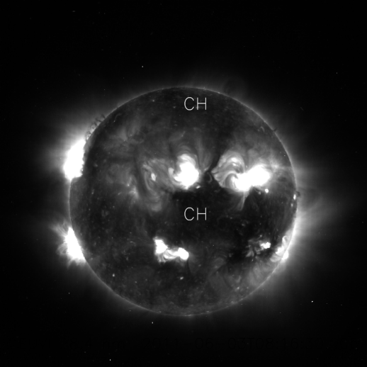
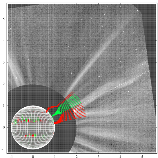
Figure 2: Upper panel: the EUV image observed at 28.4 nm by STEREO A/EUVI. On June 3 2011, STEREO A was located about 90-degree west of the Earth. Two coronal holes above and below the latitude of the wave-like feature are indicated. Lower panel: the extrapolated coronal field lines from HMI synoptic map for Carrington rotation 2110 using PFSS model. Red lines indicate inward open field lines, and green lines represent outward open field lines. The spherical source surface is set at $1.5\;R_{\odot}$.

Figure 7: The brightness distribution across the streamer at 07:24 UT along the short red lines in Figure 6 at different heliocentric distances. The distance and the corresponding ratio of the maximal to the background brightness is indicated in the upper position of each panel. Two different background models for the stray-light and F corona subtraction, that is the monthly minimum and the yearly minimum, are applied. The ratio using the yearly minimum background is indicated in the parentheses in each panel. Two parallel dotted lines represent the maximal and the background brightness. The distance along the $X$ axis is measured from the upper to lower positions on the short red line.

Figure 8: The distance-time plot of P1, P2, and P3. Linear fits indicated by solid lines are applied to derive their corresponding phase speeds, which are 406, 374 and $356\;\mathrm{kms^{-1}}$. The errorbars are the assumed $\delta=\pm 0.2\;R_{\odot}$ uncertainties. The propagation of this error to the phase speeds are indicated in the right corner as the 1-sigma uncertainty of the fitted slope.

References

- Berger et al. (2010) Berger, T. E., Slater, G., Hurlburt, N., et al. 2010, ApJ, 716, 1288
- Bettarini et al. (2006) Bettarini, L., Landi, S., Rappazzo, F. A., Velli, M., & Opher, M. 2006, A&A, 452, 321
- Bettarini et al. (2009) Bettarini, L., Landi, S., Velli, M., & Londrillo, P. 2009, Physics of Plasmas, 16, 062302
- Brueckner et al. (1995) Brueckner, G. E., Howard, R. A., Koomen, M. J., et al. 1995, Sol. Phys., 162, 357
- Chandrasekhar (1961) Chandrasekhar, S. 1961, International Series of Monographs on Physics, Oxford: Clarendon
- Chen et al. (2011) Chen, Y., Feng, S. W., Li, B., et al. 2011, ApJ, 728, 147
- Chen et al. (2009) Chen, Y., Li, X., Song, H. Q., et al. 2009, ApJ, 691, 1936
- Chen et al. (2010) Chen, Y., Song, H. Q., Li, B., et al. 2010, ApJ, 714, 644
- Dahlburg et al. (1998) Dahlburg, R. B., Boncinelli, P., & Einaudi, G. 1998, Physics of Plasmas, 5, 79
- Dahlburg et al. (2001) Dahlburg, R. B., R. Keppens, & Einaudi, G. 2001, Physics of Plasmas, 8, 1697
- Einaudi (1999) Einaudi, G. 1999, Plasma Physics and Controlled Fusion, 41, A293
- Einaudi et al. (1999) Einaudi, G., Boncinelli, P., Dahlburg, R. B., & Karpen, J. T. 1999, J. Geophys. Res., 104, 521
- Einaudi et al. (2001) Einaudi, G., Chibbaro, S., Dahlburg, R. B., & Velli, M. 2001, ApJ, 547, 1167
- Feng et al. (2012) Feng, L., Inhester, B., de Patoul, J., Wiegelmann, T., & Gan, W. Q. 2012, A&A, 538, A34
- Foullon et al. (2011) Foullon, C., Verwichte, E., Nakariakov, V. M., Nykyri, K., & Farrugia, C. J. 2011, ApJ, 729, L8
- Gary (2001) Gary, G. A. 2001, Sol. Phys., 203, 71
- Kaiser et al. (2008) Kaiser, M. L., Kucera, T. A., Davila, J. M., et al. 2008, Space Sci. Rev., 136, 5
- Lee et al. (1988) Lee, L. C., Wang, S., Wei, C. Q., & Tsurutani, B. T. 1988, J. Geophys. Res., 93, 7354
- McComas et al. (2008) McComas, D. J., Ebert, R. W., Elliott, H. A., et al. 2008, Geophys. Res. Lett., 35, 18103
- Möstl et al. (2013) Möstl, U. V., Temmer, M., & Veronig, A. M. 2013, ApJ, 766, L12
- Ofman & Thompson (2011) Ofman, L., & Thompson, B. J. 2011, ApJ, 734, L11
- Parker (1958) Parker, E. N. 1958, ApJ, 128, 664
- Ryutova et al. (2010) Ryutova, M., Berger, T., Frank, Z., Tarbell, T., & Title, A. 2010, Sol. Phys., 267, 75
- Schou et al. (2012) Schou, J., Scherrer, P. H., Bush, R. I., et al. 2012, Sol. Phys., 275, 229
- Sheeley et al. (1997) Sheeley, N. R., Jr., Wang, Y.-M., Hawley, S. H., et al. 1997, ApJ, 484, 472
- Wang et al. (1988) Wang, S., Lee, L. C., Wei, C. Q., & Akasofu, S.-I. 1988, Sol. Phys., 117, 157
- Wang et al. (1998) Wang, Y.-M., Sheeley, N. R., Jr., Socker, D. G., et al. 1998, ApJ, 508, 899
- Wang et al. (2007) Wang, Y.-M., Sheeley, N. R., Rich, N. B. 2007, ApJ, 658, 1340
- Warmuth and Mann (2005) Warmuth, A. Mann, G. 2005, Astronomy and Astrophysics 435, 1123
- Zaliznyak et al. (2003) Zaliznyak, Yu. R. Keppens, & Goedbloed, J. P. 2003, Physics of Plasmas, 10, 4478