Corrections to gauge theories in effective quantum gravity with a cutoff

Abstract

We calculate the lowest order quantum gravity contributions to QED beta function in an effective field theory picture with a momentum cutoff. We use a recently proposed 4 dimensional improved momentum cutoff that preserves gauge and Lorentz symmetries. We find that there is non-vanishing quadratic contribution to the photon 2-point function but that does not lead to the running of the original coupling after renormalization. We argue that gravity cannot turn gauge theories asymptotically free.

1 Introduction

The LHC experiments discovered a bosonic resonance consistent with the SM (Standard Model) Higgs boson with a mass approximately 126 GeV [1, 2]. This Higgs mass implies that the SM is renormalizable and might be valid up to the scale of the Planck mass [3, 4] and we live in a metastable world [5]. Only few evidences demand physics beyond the SM. The origin and properties of possible new physics motivated by dark matter and observed baryon asymmetry of the universe are still unknown. Considering the SM or its extensions valid up to the Planck scale gravitational corrections are present and can be estimated. As Einstein’s general relativity includes a dimensionful constant $\kappa$ with negative mass dimension ($\kappa^{2}=32\pi G_{\mathrm{N}}=1/M_{P}^{2}$), its perturbative quantization leads to a non-renormalizable theory, implying that the cutoff of the theory cannot be taken to infinity. Donoghue argued that assuming there is some yet unknown, well defined theory of quantum gravity that yields the observed general relativity as a low energy limit, the Einstein-Hilbert action can be used to calculate gravitational correction in the framework of effective field theories well below the Planck mass [6, 7].

The effective field theory treatment was recently used to study quantum corrections to gauge theories. Robinson and Wilczek claimed that quadratically divergent contribution to the Yang-Mills beta function is negative and points toward asymptotic freedom [10]. There were several controversial results about this statement in the literature. Pietrykowski showed in [11] that in the Maxwell-Einstein theory the result is gauge dependent. Toms repeated the calculation in the gauge choice independent background field method using dimensional regularization and has found no quadratically divergent gravity contribution to the beta function [12]. Diagrammatic calculation employing dimensional regularization and naive momentum cutoff [13] found vanishing quadratic contribution and the logarithmic divergences renormalize dimension-6 operators in agreement with the early results of Deser et al. [14]. Toms later applied proper time cutoff regularization and claimed that quadratic dependence on the energy remains in the QED one-loop effective action [15]. Analysis using the background field method employing the Vilkowsky-De Witt formalism [16, 17] and special loop regularization that respects Ward identities both found non-vanishing quadratic contributions to the beta function [16] but with sign opposite to [10, 15]. There are many various results, sometimes contradicting to each other and the physical reality of quadratic corrections to the gauge coupling was questioned [18, 19, 20]. The situation could be clarified using a cutoff calculation respecting the symmetries of the models and correctly interpreting the divergences appearing in the calculations.

Recently we developed a new improved momentum cutoff regularization which by construction respects the gauge and Lorentz symmetries of gauge theories at one loop level [21]. In this paper we apply it to the effective Maxwell-Einstein system to estimate the regularized gravitational corrections to the photon two point functions in the simplest possible model.

The paper is organized as follows. In section 2. the improved momentum cutoff is summarized, in section 3. the effective gravity contribution to quantum electrodynamics is calculated, then the renormalization is discussed. The paper is closed with conclusions and an appendix.

2 Improved momentum cutoff

A novel regularization of gauge theories is proposed in [21] based on 4 dimensional momentum cutoff to evaluate 1-loop divergent integrals. The idea was to construct a cutoff regularization which does not brake gauge symmetries and the necessary shift of the loop-momentum is allowed as no surface terms are generated. The loop calculation starts with Wick rotation, Feynman-parametrization and loop-momentum shift. Only the treatment of free Lorentz indices should be changed compared to the naive cutoff calculation.

We start with the observation that the contraction with $\eta_{\mu\nu}$ (tracing) does not necessarily commute with loop-integration in divergent cases. Therefore the substitution of

$$k_{\mu}k_{\nu}\rightarrow\frac{1}{4}\eta_{\mu\nu}k^{2}$$ (1)

is not valid under divergent integrals, where $k$ is the loop-momentum. The usual factor $1/4$ is the result of tracing both sides under a loop integral, e.g. changing the order of tracing and the integration. In the new approach the integrals with free Lorentz indices are defined using physical consistency conditions, such as gauge invariance or freedom of momentum routing. Based on the diagrammatical proof of gauge invariance it can be shown that the two conditions are related and both are in connection with the requirement of vanishing surface terms. It was proposed in [21] that instead of (1) the general identification of the cutoff regulated integrals in gauge theories

$$\int_{\Lambda\>reg}d^{4}l_{E}\frac{l_{E\mu}l_{E\nu}}{\left(l_{E}^{2}+m^{2}\right)^{n+1}}=\frac{1}{2n}\eta_{\mu\nu}\int_{\Lambda\>reg}d^{4}l_{E}\frac{1}{\left(l_{E}^{2}+m^{2}\right)^{n}},\ \ \ \ \ n=1,2,...$$ (2)

will satisfy the Ward-Takahashi identities and gauge invariance at 1-loop ($l{}_{E}$ is the shifted Euclidean loop-momentum). In case of divergent integrals it differs from (1), for non-divergent cases both substitutions give the same results at ${\cal O}(1/\Lambda^{2})$ (the difference is a vanishing surface term). It is shown in [21] that this definition is robust in gauge theories, differently organized calculations of the 1-loop functions agree with each other using (2) and disagree using (1). For four free indices the gauge invariance dictates ($n=2,3,...$)

$$\int_{\Lambda\>reg}d^{4}l_{E}\frac{l_{E\alpha}l_{E\beta}l_{E\mu}l_{E\rho}}{\left(l_{E}^{2}+m^{2}\right)^{n+1}}=\frac{1}{4n(n-1)}\int_{\Lambda\>reg}d^{4}l_{E}\frac{\eta_{\alpha\beta}\eta_{\mu\rho}+\eta_{\alpha\mu}\eta_{\beta\rho}+\eta_{\alpha\rho}\eta_{\beta\mu}}{\left(l_{E}^{2}+m^{2}\right)^{n-1}}.$$ (3)

For 6 and more free indices appropriate rules can be derived (or (2) can be used recursively for each allowed pair). Finally the scalar integrals are evaluated with a simple Euclidean momentum cutoff. The method was successfully applied to an effective model to estimate oblique corrections [22].

There are similar attempts to define a regularization that respects the original gauge and Lorentz symmetries of the Lagrangian but work in four spacetime dimensions usually with a cutoff [23, 24]. Some methods can separate the divergences of the theories and does not rely on a physical cutoff [25, 26, 27] or even could be independent of it [28]. For further literature see references in [21].

Under this modified cutoff regularization the terms with numerators proportional to the loop momentum are all defined by the possible tensor structures. Odd number of $l_{E}$’s give zero as usual, but the integral of even number of $l_{E}$ are defined by (2), (3) and similarly for more indices, this guarantees that the symmetries are not violated. The calculation is performed in 4 dimensions, the finite terms are equivalent with the results of dimensional regularization. The method identifies quadratic divergences while gauge and Lorentz symmetries are respected. We stress that the method treats differently momenta with free ($k_{\mu}k_{\nu}$) and contracted Lorentz indices ($k^{2}$), the order of tracing and performing the regulated integral cannot be changed similarly to dimensional regularization. The famous triangle anomaly can be unambiguously defined and presented in [29].

However even using dimensional regularization one is able to define cutoff results in agreement with the present method. In dimensional regularization singularities are identified as $1/\epsilon$ poles, power counting shows that these are the logarithmic divergences of the theory. Naively quadratic divergences are set to zero in the process, but already Veltman noticed that these divergences can be identified by calculating the poles in $d=2$. Careful calculation of the Veltman-Passarino 1-loop functions in dimensional regularization and with 4-momentum cutoff leads to the following identifications [21, 31, 32]

$$4\pi\mu^{2}\left(\frac{1}{\epsilon-1}+1\right) = \Lambda^{2},$$ (4)

$$\frac{1}{\epsilon}-\gamma_{E}+\ln\left(4\pi\mu^{2}\right)+1 = \ln\Lambda^{2}.$$ (5)

The finite terms are unambiguously defined

$$f_{{\rm finite}}=\lim_{\epsilon\rightarrow 0}\left[f(\epsilon)-R(0)\left(\frac{1}{\epsilon}-\gamma_{E}+\ln 4\pi+1\right)-R(1)\left(\frac{1}{\epsilon-1}+1\right)\right],$$ (6)

where $R(0)$,   $R(1)$ are the residues of the poles at $\epsilon=0,\,1$ respectively. Using (4), (5) and (6) at 1-loop the results of the improved cutoff can be reproduced using dimensional regularization without any ambiguous subtraction.

This novel momentum cutoff regularization was developed and used in gauge theories at one loop level and here it is applied to a simple system where quadratically divergent gravitational corrections could play a role.

3 Effective Maxwell-Einstein theory

The quantum corrections to the photon self energy are discussed in the Einstein-Maxwell theory

$$S=\int\mathrm{d}^{4}x\sqrt{-g}\left[\frac{2}{\kappa^{2}}R-\frac{1}{2}g^{\mu\nu}g^{\alpha\beta}F_{\mu\nu}F_{\alpha\beta}\right],$$ (7)

where $R$ is the Ricci scalar, $\kappa^{2}=32\pi G_{\mathrm{N}}$ and $F_{\mu\nu}$ denotes the $U(1)$ field strength tensor. Quantum effects are calculated in the weak field expansion around the flat Minkowski metric ($\eta_{\mu\nu}=(1,-1,-1,-1)$)

$$g_{\mu\nu}=\eta_{\mu\nu}+\kappa h_{\mu\nu}(x).$$ (8)

This is considered an exact relation, but the inverse of the metric contains higher order terms,

$$g^{\mu\nu}=\eta^{\mu\nu}-\kappa h^{\mu\nu}+\kappa^{2}h_{\alpha}^{\mu}h^{\nu\alpha}+\ldots\,,$$ (9)

in an effective treatment it can be truncated at the second order. The photon propagator is defined in Landau gauge and the graviton propagator in de Donder (harmonic) gauge, the condition is (with $h=h_{\alpha}^{\alpha}$)

$$\partial^{\nu}h_{\mu\nu}-\frac{1}{2}\partial_{\mu}h=0.$$ (10)

Expanding the Lagrangian up to second order in the graviton field the graviton propagator in $d$ dimensions is

$$G_{\alpha\beta\gamma\delta}^{G}(k)=i\frac{\frac{1}{2}\eta_{\alpha\gamma}\eta_{\beta\delta}+\frac{1}{2}\eta_{\alpha\delta}\eta_{\beta\gamma}-\frac{1}{d-2}\eta_{\alpha\beta}\eta_{\gamma\delta}}{k^{2}-i\epsilon}.$$ (11)

There are two relevant vertices involving two photons. The two photon-graviton vertex is

$$V_{\gamma\gamma G}(k_{1\mu},k_{2\nu},\alpha,\beta) \!=\! -i\frac{\kappa}{2}\left[\eta_{\alpha\beta}\left(k_{1\nu}k_{2\mu}-\eta_{\mu\nu}(k_{1}k_{2})\right)+\right.$$ (12)

$$\!\left.+Q_{\mu\nu,\alpha\beta}(k_{1}k_{2})+Q_{k_{1}k_{2},\alpha\beta}\eta_{\mu\nu}-Q_{\mu k_{2},\alpha\beta}k_{1\nu}-Q_{k_{1}\nu,\alpha\beta}k_{2\mu}\right],$$

and the two photon-two graviton vertex is even more complicated

$$V_{\gamma\gamma GG}(k_{1\mu},k_{2\nu},\alpha,\beta,\gamma,\delta) \!=\! -i\frac{\kappa^{2}}{4}\left[P_{\alpha\beta\gamma\delta}\left(k_{1\nu}k_{2\mu}-\eta_{\mu\nu}(k_{1}k_{2})\right)+U_{\mu\nu,\alpha\beta,\gamma\delta}(k_{1}k_{2})+\phantom{\kappa^{2}}\right.$$ (13)

$$\!+U_{k_{1}k_{2},\alpha\beta,\gamma\delta}\eta_{\mu\nu}-U_{\mu k_{2},\alpha\beta,\gamma\delta}k_{1\nu}-U_{k_{1}\nu,\alpha\beta,\gamma\delta}k_{2\mu}+$$

$$\!+Q_{\mu\nu,\alpha\beta}Q_{\gamma\delta,k_{1}k_{2}}+Q_{\mu\nu,\gamma\delta}Q_{\alpha\beta,k_{1}k_{2}}$$

$$\!\left.-Q_{k_{1}\nu,\alpha\beta}Q_{\mu k_{2},\gamma\delta}-Q_{\mu k_{2},\alpha\beta}Q_{k_{1}\nu,\gamma\delta}\phantom{\kappa^{2}}\right].$$

For the sake of simplicity we have defined

$$U_{\mu\nu,\alpha\beta,\gamma\delta}=\eta_{\mu\alpha}P_{\nu\beta,\gamma\delta}+\eta_{\mu\beta}P_{\alpha\nu,\gamma\delta}+\eta_{\mu\gamma}P_{\alpha\beta,\nu\delta}+\eta_{\mu\delta}P_{\alpha\beta,\gamma\nu},$$ (14)

$$P_{\alpha\beta,\mu\nu}=\eta_{\mu\alpha}\eta_{\nu\beta}+\eta_{\mu\beta}\eta_{\nu\alpha}-\eta_{\mu\nu}\eta_{\alpha\beta},$$ (15)

and finally

$$Q_{\alpha\beta,\mu\nu}=\eta_{\mu\alpha}\eta_{\nu\beta}+\eta_{\mu\beta}\eta_{\nu\alpha}.$$ (16)

There are two graphs contributing to the photon self energy (Fig. 1.) with two vertices (12) giving $\Pi^{(a)}$ and one 4-leg vertex (13) providing $\Pi^{(b)}$. We calculated the finite and divergent parts of the 2-point function with improved cutoff, naive 4-dimensional momentum cutoff and dimensional regularization. For comparison using the technique of dimensional regularization with different assumptions about treating the number of dimensions $d$ in the propagator and vertices various quadratically divergent cutoff results can be identified using (4).

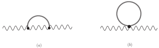
Figure 1: Feynman graphs with graviton lines contributing to the photon two point function.

The $\Lambda^{2}$ contributions of the two graphs with improved cutoff (I) do not cancel each other

$$\Pi_{\mu\nu}^{\mathrm{I}(a)}(p) = \frac{i}{16\pi^{2}}\kappa^{2}\left(p^{2}\eta_{\mu\nu}-p_{\mu}p_{\nu}\right)\left(-2\Lambda^{2}-\frac{1}{6}p^{2}\left(\ln\left(\frac{\Lambda^{2}}{p^{2}}\right)+\frac{2}{3}\right)\right),$$ (17)

$$\Pi_{\mu\nu}^{\mathrm{I}(b)}(p) = \frac{i}{16\pi^{2}}\kappa^{2}\left(p^{2}\eta_{\mu\nu}-p_{\mu}p_{\nu}\right)\left(\phantom{2}\frac{3}{2}\Lambda^{2}\right).$$ (18)

In the naive cutoff (N) calculation using (1) there is a cancellation of the $\Lambda^{2}$ terms, the finite term differs from the previous one and it is impressing that the result is transverse without any subtractions

$$\Pi_{\mu\nu}^{\mathrm{N}(a)}(p) = \frac{i}{16\pi^{2}}\kappa^{2}\left(p^{2}\eta_{\mu\nu}-p_{\mu}p_{\nu}\right)\left(-\frac{3}{2}\Lambda^{2}-\frac{1}{6}p^{2}\ln\left(\frac{\Lambda^{2}}{p^{2}}\right)-\frac{7}{36}p^{2}\right),$$ (19)

$$\Pi_{\mu\nu}^{\mathrm{N}(b)}(p) = \frac{i}{16\pi^{2}}\kappa^{2}\left(p^{2}\eta_{\mu\nu}-p_{\mu}p_{\nu}\right)\left(\phantom{-}\frac{3}{2}\Lambda^{2}\right).$$ (20)

In dimensional regularization (DR) the space-time dimension is continued in all terms originating from the gauge and gravitational part, too (e.g. $\eta_{\mu}^{\mu}=d=4-2\epsilon$). The result agrees with [13] (without the finite terms which are first given here)

$$\Pi_{\mu\nu}^{DR1(a)}(p) = \frac{i}{16\pi^{2}}\kappa^{2}\left(p^{2}\eta_{\mu\nu}-p_{\mu}p_{\nu}\right)\left(-\frac{1}{6}p^{2}\left(\frac{2}{\epsilon}+\ln\left(\frac{\mu^{2}}{p^{2}}\right)+\frac{1}{6}\right)\right),$$ (21)

$$\Pi_{\mu\nu}^{DR1(b)}(p) = 0,$$ (22)

where we have omitted the constants $-\gamma_{E}+\ln 4\pi$ beside $2/\epsilon$. In what follows the various results using the technique of dimensional regularization based on different assumptions are denoted by the superscript $DR1,\,DR2,\,DR3$ and the corresponding cutoff results by $\Lambda 1,\,\Lambda 2,\,\Lambda 3$.

Now with the help of the equations (4), (5) and (6) we can define a cutoff result based on the dimensional regularization one. In principle the dimension has to be modified in each terms where $d$ appears, also in the graviton propagator (11), though gravity is not a dynamical theory in $d=2$. Each graph is quadratically divergent, even $1/(\epsilon-1)^{2}$ type of singularities appear in single graphs, but they cancel in the sum of the graphs, like the $\frac{1}{\epsilon^{2}}$ terms in usual gauge theories (e.g. in QCD) at two loops.

$$\Pi_{\mu\nu}^{\mathrm{\Lambda 1}}(p)=\frac{i}{16\pi^{2}}\kappa^{2}\left(p^{2}\eta_{\mu\nu}-p_{\mu}p_{\nu}\right)\left(-\frac{1}{4}\Lambda^{2}-\frac{1}{6}p^{2}\left(\ln\left(\frac{\Lambda^{2}}{p^{2}}\right)-\frac{5}{6}\right)\right)$$ (23)

also quadratically divergent, but only the coefficient of the logarithmic term agrees with other results.

The result of the improved momentum cutoff can be reproduced applying dimensional regularization with care. The improved cutoff method works in four physical dimensions and special rules have to be applied only at the evaluation of the last tensor integrals. It is equivalent to setting $d=4$ in the Einstein-Maxwell theory, e.g. both in the graviton propagator and in the trace of the metric tensor. Dimensional regularization is then applied at the last step evaluating the tensor and scalar momentum integrals. We have found that $\Pi_{\mu\nu}^{\mathrm{DR2(b)}}=0$ and

$$\Pi_{\mu\nu}^{DR2}(p)=\frac{i}{16\pi^{2}}\kappa^{2}\left(p^{2}\eta_{\mu\nu}-p_{\mu}p_{\nu}\right)\left(-\frac{1}{6}p^{2}\left(\frac{2}{\epsilon}+\ln\left(\frac{\mu^{2}}{p^{2}}\right)+\frac{5}{3}\right)\right).$$ (24)

The corresponding cutoff result diverges quadratically and agrees with the improved cutoff calculation

$$\Pi_{\mu\nu}^{\mathrm{\Lambda 2}(a)}(p) = \frac{i}{16\pi^{2}}\kappa^{2}\left(p^{2}\eta_{\mu\nu}-p_{\mu}p_{\nu}\right)\left(-2\Lambda^{2}-\frac{1}{6}\left(p^{2}\ln\left(\frac{\Lambda^{2}}{p^{2}}\right)+\frac{2}{3}\right)\right),$$ (25)

$$\Pi_{\mu\nu}^{\mathrm{\Lambda 2}(b)}(p) = \frac{i}{16\pi^{2}}\kappa^{2}\left(p^{2}\eta_{\mu\nu}-p_{\mu}p_{\nu}\right)\left(\phantom{2}\frac{3}{2}\Lambda^{2}\right).$$ (26)

To find connection with existing, partially controversial literature, we have performed the calculation with weaker assumptions. First the term in the graviton propagator is set $\frac{1}{d-2}=\frac{1}{2}$ as is usually done in earlier results e.g. [19, 20]. The divergent part of the dimensional regularization result agrees with [13]. The contribution of the tadpole in Fig. 1b $\Pi^{\mathrm{DR3(b)}}$ vanishes, the sum is

$$\Pi_{\mu\nu}^{DR3}(p)=\frac{i}{16\pi^{2}}\kappa^{2}\left(p^{2}\eta_{\mu\nu}-p_{\mu}p_{\nu}\right)\left(-\frac{1}{6}p^{2}\left(\frac{2}{\epsilon}+\ln\left(\frac{\mu^{2}}{p^{2}}\right)+\frac{1}{6}\right)\right).$$ (27)

We can identify a cutoff result, Fig. 1b gives $\Pi_{\mu\nu}^{\mathrm{\Lambda 3(b)}}(p)\sim\frac{1}{2}\Lambda^{2}$, the only quadratically divergent term,

$$\Pi_{\mu\nu}^{\mathrm{\Lambda 3}}(p)=\frac{i}{16\pi^{2}}\kappa^{2}\left(p^{2}\eta_{\mu\nu}-p_{\mu}p_{\nu}\right)\left(\frac{1}{2}\Lambda^{2}-\frac{1}{6}p^{2}\left(\ln\left(\frac{\Lambda^{2}}{p^{2}}\right)-\frac{5}{6}\right)\right).$$ (28)

Notice that this result differs from (23) only in the coefficient of the first term, the change comes from the different treatment of the graviton propagator.

In principle a theory is completely defined via specifying the Lagrangian and the method of calculation e.g. fixing the regularization and the treatment of the divergent terms, though the physical quantities must be independent of the details. It is remarkable that the transverse structure of the photon propagator is not violated in any of the previous regularizations and the logarithmic term is universal and agrees with earlier results [13, 14]. The question is whether the $\Lambda^{2}$ terms contribute to the running of the gauge coupling, or not.

4 Quadratic divergences and renormalization

The 1-loop corrections to the 2-point function modify the bare Lagrangian, the divergences have to be removed by the counterterms. Consider the QED action with the convention [33]

$$L_{0}=-\frac{1}{4e_{0}^{2}}F_{\mu\nu}F^{\mu\nu}+\bar{\Psi}iD_{\mu}\gamma^{\mu}\Psi,\qquad D_{\mu}=\partial_{\mu}+iA_{\mu}.$$ (29)

The divergences calculated from the interaction (7) modify the bare Lagrangian

$$L=-\frac{1+a\kappa^{2}\Lambda^{2}}{4e_{0}^{2}}F_{\mu\nu}F^{\mu\nu}+a_{2}\ln\frac{\Lambda^{2}}{p^{2}}\left(D_{\mu}F^{\mu\nu}\right)^{2}+\left(\bar{\Psi}iD_{\mu}\gamma^{\mu}\Psi,\right),$$ (30)

where $p^{2}$ is the Euclidean momentum at which the 2-point function was calculated.

The divergent terms have to be canceled by the counterterms. New dimension-six term must be added to match the $p^{2}\ln\left(\frac{\Lambda^{2}}{p^{2}}\right)$ term,

$$L_{\mathrm{\mathrm{ct}}}=\frac{\delta Z_{1}}{4e_{0}^{2}}F_{\mu\nu}F^{\mu\nu}+\delta Z_{2}\left(D_{\mu}F^{\mu\nu}\right)^{2}.$$ (31)

In principle there are three possible dimension-six counterterms, two of them linearly independent and it turns out that the second term in (31) can cancel all divergences. The coefficient of the first term in (30) cannot be understood as defining a running coupling but it is compensated by a counterterm through a renormalization condition. It can be fixed either by the Coulomb potential or Thomson scattering at low energy identifying the usual electric charge as

$$\frac{e_{0}^{2}}{4\pi(1+a\kappa^{2}\Lambda^{2})}=\frac{e^{2}}{4\pi}\simeq\frac{1}{137}.$$ (32)

The quadratically divergent correction defines the relation between the bare charge $e_{0}(\Lambda)$ in a theory with the physical cutoff $\Lambda$ and the physical charge effective at low energies. After fixing the parameters of the theory (e.g. by a measurement at low energy) and using $e$ to calculate the predictions of the model the cutoff dependence completely disappears from the physical charge [19, 33]. The role of the quadratic correction is to define the relation(32) and to renormalize the bare coupling constant $e_{0}(\Lambda)$. ( and does not appear in the physical charge.)

The logarithmically divergent contribution on the other hand defines the renormalization of the higher dimensional operator $\left(D_{\mu}F^{\mu\nu}\right)^{2}$ and again not the running of the gauge coupling. After renormalization (at a point $p^{2}=\mu^{2}$) the logarithmic coefficient of the dim-6 term in(30) changes to $a_{2}\ln\frac{\Lambda^{2}}{p^{2}}-a_{2}\ln\frac{\Lambda^{2}}{\mu^{2}}=-a_{2}\ln\frac{p^{2}}{\mu^{2}}$ defining a would be running parameter. Furthermore note that[13, 18] this term can be removed by local field redefinition of $A_{\mu}$ up to higher dimensional operators

$$A_{\mu}\rightarrow A_{\mu}-c\nabla_{\nu}F_{\mu}^{\nu},$$ (33)

where $\nabla_{\mu}$ is the gravitational covariant derivative, as the new term is proportional to the tree level equation of motion $D_{\mu}F^{\mu\nu}=0$. Generally, all photon propagator corrections can be removed by appropriate field redefinition which are bilinear in $A_{\mu}$ even if they contain arbitrary number of derivatives, on-shell scattering processes are not influenced by the presence of such effective terms [34] .

5 Conclusions

We have calculated the gravitational corrections to the simplest, $U(1)$ gauge theory. This paper was motivated by the various, sometime controversial results in the literature. Our method was capable of identifying quadratically divergent contributions to the photon two point function, thanks to the construction in a gauge invariant way. To test our calculation we defined the cutoff dependence employing (4),(5) anddimensional regularization with various assumptions about treating the number of dimensions $d$. We observed that the 1-loop gravity corrections to the two point function in all but one cases contain $\Lambda^{2}$ divergence with the exception of the naive momentum cutoff which violates gauge symmetries usually. Here all the corrections are transverse and the logarithmic term universally agrees with the literature starting from Deser et al. [14].

The quadratically divergent corrections to the photon self-energy do not lead to the modification of the running of the gauge coupling. Robinson and Wilczek claimed that the $-a\kappa^{2}\Lambda^{2}$ correction could turn the beta function negative and make the Maxwell-Einstein theory asymptotically free. This statement and the calculation was criticized in the literature. We showed in this paper using explicit cutoff calculation that $\Lambda^{2}$ corrections do appear in the 2-point function, but those will define the renormalization connection between the cutoff dependent bare coupling and the physical coupling (32) and do not lead to a running coupling. Indeed the $\Lambda^{2}$ correction absorbed into the physical charge and does not appear in physical processes. Donoghue et al. argue in [19] that a universal, i.e. process independent running coupling constant cannot be defined in the effective theory of gravity independently of the applied regularization. They demonstrate that because of the crossing symmetry in theories (except the $\lambda\Phi^{4}$) even the sign of the quadratic running is ambiguous and a running coupling would be process dependent. Generally the logarithmically divergent corrections could define the renormalization of higher dimensional operators. It turns out that even these logarithmic correction can be removed by appropriate field redefinitions and do not contribute to on-shell scattering processes. We note that the authors in [20] showed using their 4-dimensional implicit regularization method that the quadratic terms are coming from ambiguous surface terms and as such are non-physical. Interestingly those surface terms vanish if we evaluate them with our improved cutoff.

Finally we point out that we have found gravity corrections to the two point function of the $U(1)$ gauge theory. Using a momentum cutoff the quadratically divergent contributions define the renormalization of the bare charge and thus using the physical charge the $\Lambda^{2}$ corrections do not appear in physical processes. On the other hand logarithmic corrections are universal but merely define the renormalization of a dimension six term in the Lagrangian, which term can be eliminated by local field redefinition. We conclude that gravity corrections do not lead to the modification of the usual running of gauge coupling and cannot point towards asymptotic freedom in the case of electromagnetism.

Appendix A The divergent integrals

The loop integrals are calculated as follows. First the loop momentum ($k$) integral is Wick rotated (to $k_{E}$), with Feynman parameter(s) the denominators are combined, then the order of Feynman parameter and the momentum integrals are changed. After that the loop momentum ($k_{E}\rightarrow l_{E}$) is shifted to have a spherically symmetric denominator.

In this appendix we present two divergent integrals calculated by the new regularization. $\Delta$ can be any loop momentum independent expression depending on the Feynman $x$ parameter, external momenta, masses, e.g. $\Delta(x,q_{i},m).$ The integration is understood for Euclidean momenta with absolute value below $\Lambda$.

The integral (34) is just given for comparison, it is calculated with a simple momentum cutoff. In (35) with the standard (1) substitution one would get a constant $-\frac{3}{2}$ instead of $-1$ [21].

$$\int_{\Lambda\,reg}\frac{d^{4}l_{E}}{i(2\pi)^{4}}\frac{1}{\left(l_{E}^{2}+\Delta^{2}\right)^{2}} \!\!=\!\! \frac{1}{(4\pi)^{2}}\left(\ln\left(\frac{\Lambda^{2}+\Delta^{2}}{\Delta^{2}}\right)+\frac{\Delta^{2}}{\Lambda^{2}+\Delta^{2}}-1\right).$$ (34)

$$\int_{\Lambda\,reg}\frac{d^{4}k}{i(2\pi)^{4}}\frac{l_{E\mu}l_{E\nu}}{\left(l_{E}^{2}+\Delta^{2}\right)^{3}} \!\!=\!\! \frac{1}{(4\pi)^{2}}\frac{g_{\mu\nu}}{4}\left(\ln\left(\frac{\Lambda^{2}+\Delta^{2}}{\Delta^{2}}\right)+\frac{\Delta^{2}}{\Lambda^{2}+\Delta^{2}}-1\right).$$ (35)

References

- [1] G. Aad et al. [ATLAS Collaboration], Phys. Lett. B 716 (2012) 1.
- [2] S. Chatrchyan et al. [CMS Collaboration], Phys. Lett. B 716 (2012) 30.
- [3] G. Degrassi, S. Di Vita, J. Elias-Miro, J. R. Espinosa, G. F. Giudice, G. Isidori and A. Strumia, JHEP 1208 (2012) 098.
- [4] F. Bezrukov, M. Y. Kalmykov, B. A. Kniehl and M. Shaposhnikov, JHEP 1210 (2012) 140.
- [5] D. Buttazzo, G. Degrassi, P. P. Giardino, G. F. Giudice, F. Sala, A. Salvio and A. Strumia, arXiv:1307.3536 [hep-ph].
- [6] J. F. Donoghue, Phys. Rev. D 50 (1994) 3874.
- [7] J. F. Donoghue, AIP Conf. Proc. 1483 (2012) 73.
- [8] G. ’t Hooft and M. J. G. Veltman, Nucl. Phys. B 44 (1972) 189.
- [9] J. Collins, Renormalization, Cambridge University Press, 1984.
- [10] S. P. Robinson and F. Wilczek, Phys. Rev. Lett. 96 (2006) 231601.
- [11] A. R. Pietrykowski, Phys. Rev. Lett. 98 (2007) 061801.
- [12] D. J. Toms, Phys. Rev. D 76 (2007) 045015.
- [13] D. Ebert, J. Plefka and A. Rodigast, Phys. Lett. B 660 (2008) 579.
- [14] S. Deser, H. -S. Tsao and P. van Nieuwenhuizen, Phys. Rev. D 10 (1974) 3337.
- [15] D. J. Toms, Nature 468 (2010) 56.
- [16] Y. Tang and Y. -L. Wu, Commun. Theor. Phys. 57 (2012) 629.
- [17] A. R. Pietrykowski, Phys. Rev. D 87 (2013) 024026.
- [18] J. Ellis and N. E. Mavromatos, Phys. Lett. B 711 (2012) 139.
- [19] M. M. Anber, J. F. Donoghue and M. El-Houssieny, Phys. Rev. D 83 (2011) 124003.
- [20] J. C. C. Felipe, L. C. T. Brito, M. Sampaio and M. C. Nemes, Phys. Lett. B 700 (2011).
- [21] G. Cynolter and E. Lendvai, Central Eur.J.Phys. 9 (2011) 1237.
- [22] G. Cynolter, E. Lendvai and G. Pócsik, Mod. Phys. Lett. A 24 (2009) 2331.
- [23] Y. Gu, J. Phys. A 39 (2006) 13575.
- [24] Y. L. Wu, Int. J. Mod. Phys. A 18 (2003) 5363.
- [25] O. A. Battistel and M. C. Nemes, Phys. Rev. D 59 (1999) 055010.
- [26] S. Arnone, T. R. Morris and O. J. Rosten, Eur. Phys. J. C 50 (2007) 467.
- [27] F. del Aguila and M. Perez-Victoria, Acta Phys. Polon. B 29 (1998) 2857.
- [28] R. Pittau, JHEP 1211 (2012) 151.
- [29] G. Cynolter and E. Lendvai, Mod. Phys. Lett. A 26 (2011) 1537.
- [30] M.J.G Veltman, Acta Phys. Polon. B12: (1981) 437.
- [31] K. Hagiwara, S. Ishihara, R. Szalapski and D. Zeppenfeld, Phys. Rev. D 48 (1993) 2182.
- [32] M. Harada and K. Yamawaki, Phys. Rev. D 64, 014023 (2001).
- [33] M. M. Anber and J. F. Donoghue, Phys. Rev. D 85 (2012) 104016.
- [34] A. A. Tseytlin, Phys. Lett. B 176 (1986) 92.