LA-UR-13-24956 BPHZ renormalization and its application
to non-commutative field theory

Abstract

In a recent work a modified BPHZ scheme has been introduced and applied to one-loop Feynman graphs in non-commutative $\phi^{4}$-theory. In the present paper, we first review the BPHZ method and then we apply the modified BPHZ scheme as well as Zimmermann’s forest formula to the sunrise graph, i.e. a typical higher-loop graph involving overlapping divergences. Furthermore, we show that the application of the modified BPHZ scheme to the IR-singularities appearing in non-planar graphs (UV/IR mixing problem) leads to the introduction of a $1/{p}^{\,2}$ term and thereby to a renormalizable model. Finally, we address the application of this approach to gauge field theories.

1 Introduction

In this work we continue the discussion of the BPHZ renormalization of non-commutative $\phi^{4}$-theory in four Euclidean dimensions initiated in reference [1] and we address in particular the issue of higher-loop graphs involving overlapping divergences. The theory under consideration is defined at the classical level by the action (e.g. see reference [2])

$$\Gamma^{(0)}[\phi]=\Gamma^{(0)}_{\text{free}}[\phi]+\Gamma^{(0)}_{\text{int}}[\phi]\equiv\frac{1}{2}\int d^{4}x\left(\partial^{\mu}\phi\star\partial_{\mu}\phi+m^{2}\,\phi\star\phi\right)\,+\,\frac{\lambda}{4!}\int d^{4}x\left(\phi\star\phi\star\phi\star\phi\right)\,.$$ (1)

From the definition of the Moyal star product,

$$\left(f\star g\right)(x):=\left({\rm e}^{\frac{{\rm i}}{2}\theta^{\mu\nu}\partial^{x}_{\mu}\partial^{y}_{\nu}}f(x)g(y)\right)\Big{|}_{x=y}\,,\qquad{\rm with}\ \;\theta^{\mu\nu}=-\theta^{\nu\mu}\ \;{\rm constant}\,,$$ (2)

it follows that

$$\Gamma^{(0)}[\phi]=\int d^{4}x\left[\frac{1}{2}(\partial^{\mu}\phi\,\partial_{\mu}\phi+m^{2}\phi^{2})+\frac{\lambda}{4!}\,(\phi\star\phi\star\phi)(x)\,\phi(x)\right]\,.$$ (3)

Introducing the Fourier components $\tilde{\phi}(k)$ of $\phi$ by $\phi(x)=\frac{1}{(2\pi)^{4}}\int d^{4}k\,{\rm e}^{{\rm i}kx}\tilde{\phi}(k)$, we find that the propagator in momentum space is given by

$$\tilde{\Delta}(k)=\frac{1}{k^{2}+m^{2}}\,,$$ (4)

and that the interaction term can be expressed in terms of the variables $\tilde{k}_{\mu}\equiv\theta_{\mu\nu}k^{\nu}$ by

$$\Gamma^{(0)}_{\text{int}}[\phi]=\frac{1}{4!}\int\!d^{4}k_{1}\ldots d^{4}k_{4}\,\tilde{\phi}(k_{1})\tilde{\phi}(k_{2})\tilde{\phi}(k_{3})\tilde{\phi}(k_{4})\,(2\pi)^{4}\,\delta^{(4)}(k_{1}+k_{2}+k_{3}+k_{4})\,\bar{\lambda}\,,$$

with

$$\bar{\lambda}\equiv\frac{\lambda}{3}\bigg{[}\cos\frac{k_{1}\tilde{k}_{2}}{2}\cos\frac{k_{3}\tilde{k}_{4}}{2}+\cos\frac{k_{1}\tilde{k}_{3}}{2}\cos\frac{k_{2}\tilde{k}_{4}}{2}+\cos\frac{k_{1}\tilde{k}_{4}}{2}\cos\frac{k_{2}\tilde{k}_{3}}{2}\bigg{]}\,.$$ (5)

Henceforth, in comparison to the commutative $\phi^{4}$-theory, the interaction vertex of the non-commutative $\phi^{4}$-theory is characterized by a modified coupling in momentum space ($\lambda$ becomes $\bar{\lambda}$).

The quantization of this model and the renormalization of related scalar field models has been discussed over the last fifteen years, see for instance reference [1] for a brief review and list of references. In the latter work it was pointed out that the usual BPHZ momentum space subtraction scheme (which consists of subtracting appropriate polynomials in the external momentum from the integrand of divergent integrals) cannot be applied in non-commutative theories, e.g. for an integral of the form

$$J(p)\equiv\int\!d^{4}k\,\frac{\cos(k\tilde{p})}{[(p+k)^{2}+m^{2}][k^{2}+m^{2}]}\,.$$ (6)

The problem is due to the phase factor $\cos(k\tilde{p})$ which is at the origin of the UV/IR mixing problem, i.e. the appearance of an IR-singularity for small values of the external momentum $p$. Therefore, a modified subtraction scheme was proposed in reference [1]: it consists of considering $p$ and $\tilde{p}$ as independent variables (though satisfying $p\tilde{p}=0$) when performing the subtraction, i.e. one subtracts from the integrand its Taylor series expansion with respect to the external momentum $p$ around $p=0$ up to the order of divergence of the graph, while maintaining the phase factors: thus, for the integral (6) one considers

$$J^{{\rm finite}}(p)\equiv\int\!d^{4}k\left(\frac{\cos(k\tilde{p})}{[(p+k)^{2}+m^{2}][k^{2}+m^{2}]}-\frac{\cos(k\tilde{p})}{[k^{2}+m^{2}]^{2}}\right)\,.$$ (7)

By proceeding in this way, the one-loop renormalization of the theory could be carried out for the so-called naïve $\phi^{4}$-theory described by the action (1) as well as for this action supplemented by a $1/p^{2}$-term which is known to overcome the UV/IR mixing problem while maintaining the translation invariance of the model [3].

Part of the present work concerns the application of the modified subtraction scheme to higher-loop graphs involving overlapping divergences. For concreteness, we will investigate in detail the sunrise graph as an example for a two-loop graph with overlapping divergences. To tackle this problem, we apply the so-called forest formula of Zimmermann [4] in the non-commutative setting using the modified subtraction scheme.

In this context, it is worthwhile recalling that an open problem in non-commutative field theories is that there exists no proof for the renormalizability of the proposed classical gauge field models. Indeed, the methods considered so far for the quantization of scalar field theories on non-commutative space (such as multi-scale analysis) cannot be applied, or at least not without some serious complications, to gauge field theories due to the fact that they break the gauge symmetry. This is a strong impetus for trying to generalize to the non-commutative setting the approach of BPHZ which does not require the introduction of a regularization and which has been proven to be a powerful tool for field theories with local symmetries on commutative space, e.g. see references [5, 6]. With this motivation in mind and in order to present a self-contained treatment of the sunrise-graph, we provide a short introduction to the BPHZ-approach to renormalization in Section 2 before treating the sunrise-graph of non-commutative $\phi^{4}$-theory in Section 3.3 and discussing IR-singularities in Section 3.1. We conclude with some comments on gauge theories and the issues to be addressed in future work.

2 BPHZ in a nutshell

In this section we present a sketch of the BPHZ (Bogoliubov, Parasiuk, Hepp, Zimmermann) method of renormalization in Euclidean $\mathds{R}^{4}$ which is based on some ideas put forward by Stueckelberg and Green [7, 8]. The original references are [9, 10, 11, 12, 13, 14][4][15] and the approach has been conveniently reformulated by Zimmermann [14, 4, 16], different aspects being discussed in references [17, 18, 19, 20, 21, 22, 23, 24, 25, 26, 27, 28, 29, 30, 31, 32].

2.1 Generalities

The BPHZ approach to the perturbative renormalization of field theory amounts to a proper definition of the quantum theory and essentially consists of three ingredients:

1. A subtraction scheme, i.e a systematic procedure for subtracting an overall ultraviolet divergence as well as subdivergences (i.e. divergences of subdiagrams) from any Feynman integral (1PI (one-particle-irreducible) graph or function) in order to get a finite (convergent) expression for this integral.

2. A proof of the locality of these subtractions, i.e. a proof that these subtractions correspond to the addition of local counterterms to the Lagrangian having the same form as those in the original Lagrangian (compatibility with additive renormalization).

3. A set of normalization conditions on the 1PI functions involving divergences in order to fix the physical parameters (masses, coupling constants, …) of the theory. These conditions can be achieved by the addition of finite counterterms to the Lagrangian.

If the initial Lagrangian has some rigid or local symmetries, these also have to be taken into account, i.e. the counterterms have to be invariant (and if a regularization is chosen for performing the subtractions, it has to respect the symmetries). A systematic method for implementing this program is provided by the method of algebraic renormalization [5, 6].

In the BPHZ approach, the subtraction of divergences can be performed by considering a particular regularization (such as dimensional regularization) or without using such a regularization (momentum space subtraction in the integrands of Feynman integrals). The latter approach allows to treat in particular field theories for which no invariant regulator is known.

In the BPHZ method, the systematic subtraction of subdivergences for a given graph is realized by Zimmermann’s forest formula which yields finite (i.e. renormalized) Feynman integrals. The fact that the latter formula represents a solution of the recursion relation for Bogoliubov’s $R$-operation allows to prove inductively the locality of the subtractions. Thus, the BPHZ approach to renormalization is equivalent to the familiar method based on counterterms. Different renormalization schemes are always related by a finite renormalization.

2.2 Subtraction operator

Suppose we have an integral $J_{\Gamma}$ corresponding to an amputated 1PI Feynman diagram $\Gamma$ which has an overall divergence, but no subdivergence. (The treatment of graphs containing divergent subgraphs will be addressed in Subsection 2.5.) An example [5] concerning the $\phi^{4}$-theory in Euclidean $\mathds{R}^{4}$ is given by the one-loop four-point 1PI graph (the so-called fish diagram depicted in Fig. 1) depending on the total incoming external momentum $p=p_{1}+p_{2}=p_{3}+p_{4}$:

$$J_{\Gamma}(p)\equiv\int\!d^{4}k\,\tilde{\Delta}(p+k)\,\tilde{\Delta}(-k)=\int\!d^{4}k\,\frac{1}{[(p+k)^{2}+m^{2}][k^{2}+m^{2}]}\equiv\int\!d^{4}k\,I_{\Gamma}(p,k)\,.$$ (8)

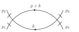
Figure 1: The fish diagram

This integral is logarithmically divergent, i.e. the superficial degree of divergence $\delta(\Gamma)$ of the graph $\Gamma$ vanishes. A finite part for such an integral satisfying $\delta(\Gamma)\geq 0$ can be extracted in different manners. Quite generally, for an integral $J_{\Gamma}(\underline{p})\equiv\int\!d^{4}k\,I_{\Gamma}(\underline{p},k)$ depending on the external momenta $\underline{p}\equiv(p_{1},\dots,p_{n})$ with $p_{1}+\dots+p_{n}=0$, the BPHZ momentum space subtraction is defined by

$$\framebox{\mbox{$\ J_{\Gamma}^{{\rm finite}}(\underline{p})\equiv\int\!d^{4}k\,\left[1-t_{\underline{p}}^{\delta(\Gamma)}\right]\,I_{\Gamma}(\underline{p},k)\ $}}\,,$$ (9)

where the Taylor expansion operator (acting on the integrand of the graph $\Gamma$) is given by

$$\left(t_{\underline{p}}^{N}I_{\Gamma}\right)(\underline{p},k)\equiv\sum_{l=0}^{N}\frac{1}{l!}\,p_{i_{1}}^{\mu_{1}}\cdots p_{i_{l}}^{\mu_{l}}\,\frac{\partial^{l}I_{\Gamma}}{\partial p_{i_{1}}^{\mu_{1}}\cdots\partial p_{i_{l}}^{\mu_{l}}}\big{(}\underline{p}=\underline{0},k\big{)}\,.$$ (10)

In particular, for a single external momentum, i.e. $\underline{p}=p$, one has

$$\left(t_{p}^{N}I_{\Gamma}\right)(p,k)=I_{\Gamma}(0,k)+p^{\mu}\,\frac{\partial I_{\Gamma}}{\partial p^{\mu}}\big{(}0,k\big{)}+\dots+\frac{1}{N!}\,p^{\mu_{1}}\cdots p^{\mu_{N}}\,\frac{\partial^{N}I_{\Gamma}}{\partial p^{\mu_{1}}\cdots\partial p^{\mu_{N}}}\big{(}0,k\big{)}\,.$$ (11)

Thus, for the integral (8), we obtain

$$J_{\Gamma}^{{\rm finite}}(p)\equiv\int\!d^{4}k\,[1-t_{p}^{0}]\,I_{\Gamma}(p,k) =\int\!d^{4}k\,[I_{\Gamma}(p,k)-I_{\Gamma}(0,k)]$$ (12)

$$=\int\!d^{4}k\,\left(\frac{1}{[(p+k)^{2}+m^{2}][k^{2}+m^{2}]}-\frac{1}{[k^{2}+m^{2}]^{2}}\right)\,,$$

which represents a convergent integral. In this respect, we note that $I_{\Gamma}(p,k)-I_{\Gamma}(0,k)=p^{\mu}\,\frac{\partial I_{\Gamma}}{\partial p^{\mu}}\big{(}0,k\big{)}+\cdots$ and that the differentiation with respect to $p^{\mu}$ lowers the degree of divergence of the propagator and thereby of the integral. For the logarithmically divergent integral (8), the first derivative already renders the integral UV-convergent:

$$\frac{\partial J_{\Gamma}}{\partial p^{\mu}}\big{(}p\big{)}=-\int\!d^{4}k\,\frac{2(p+k)_{\mu}}{[(p+k)^{2}+m^{2}]^{2}\,[k^{2}+m^{2}]}\sim\int\frac{dK\,K^{4}}{K^{6}}\sim K^{-1}\,.$$ (13)

In fact [5], the latter expression may be taken as the definition of the renormalized integral associated to $J_{\Gamma}(p)$; since it follows from (12) that $\frac{\partial J_{\Gamma}^{{\rm finite}}}{\partial p^{\mu}}(p)=\frac{\partial J_{\Gamma}}{\partial p^{\mu}}(p)$, we conclude that $J_{\Gamma}^{{\rm finite}}$ is only defined up to a real constant $d$. (Equivalently, we can argue that the Taylor series expansion of $[1-t_{p}^{0}]\,I_{\Gamma}(p,k)$ with respect to $p^{\mu}$ vanishes to order zero.) Henceforth, we have the freedom of considering

$$J_{\Gamma}^{{\rm finite}}(p)\leadsto J_{\Gamma}^{{\rm finite}}(p)+d\,,\qquad(d\in\mathds{R})\,.$$ (14)

From the fact that $J_{\Gamma}(p)$ represents the one-loop four-point function, one concludes that the addition (14) in momentum space amounts to adding to the Lagrangian a finite counterterm having the same form as the original interaction term:

$${\cal L}\leadsto{\cal L}+d\,\phi^{4}\,.$$ (15)

This counterterm originating from the one-loop subtraction, is of order $\hbar$.

Summarizing the considered example and coming back to the general case of an integral $J_{\Gamma}(p)\equiv\int\!d^{4}k\,I_{\Gamma}(p,k)$ with superficial degree of divergence $\delta(\Gamma)$, we can say the following. The operation $t_{p}^{\delta(\Gamma)}$ allows to extract from the integrand $I_{\Gamma}$ the divergent part of the integral $J_{\Gamma}$: this part is a polynomial in the external momenta whose order coincides with the degree of divergence $\delta(\Gamma)$ of the graph $\Gamma$. The operator

$$R_{\Gamma}\equiv 1-t_{p}^{\delta(\Gamma)}$$ (16)

which extracts a finite part from $J_{\Gamma}$ is Bogoliubov’s $R$-operation for the case of an integral having only an overall divergence (which we consider in this subsection). The renormalized integral associated to $J_{\Gamma}$ can be defined as its momentum space derivative of order $\delta(\Gamma)+1$ which represents a convergent integral. The extraction of a finite part from $J_{\Gamma}(p)$ by means of Bogoliubov’s $R$-operation yields the expression $J_{\Gamma}^{{\rm finite}}(p)$ which is only determined up to a polynomial in $p$ of degree $\delta(\Gamma)$:

$$J_{\Gamma}^{{\rm finite}}(p)\leadsto J_{\Gamma}^{{\rm finite}}(p)+\sum_{l=0}^{\delta(\Gamma)}\frac{1}{l!}\,d_{\mu_{1}\dots\mu_{l}}\,p^{\mu_{1}}\cdots p^{\mu_{l}}\,.$$ (17)

In configuration space the latter polynomial in $p$ corresponds to finite local counterterms involving $\partial^{\mu_{1}}\phi,\dots,\partial^{\mu_{l}}\phi$.

It is instructive [5] to investigate the one-loop two-point 1PI graph of the $\phi^{4}$-theory (the so-called tadpole graph) from this viewpoint since it does not depend on the external momentum and is quadratically divergent (i.e. $\delta(\Gamma)=2$): up to a constant factor, it is given by

$$J_{\Gamma}=\int\frac{d^{4}k}{k^{2}+m^{2}}\equiv\int\!d^{4}k\,I_{\Gamma}(p,k)\,.$$ (18)

Application of the BPHZ subtraction scheme yields a vanishing result:

$$J_{\Gamma}^{{\rm finite}}\equiv\int\!d^{4}k\,[1-t_{p}^{2}]\,I_{\Gamma}(p,k)=\int\!d^{4}k\,[I_{\Gamma}(p,k)-I_{\Gamma}(0,k)]=0\,.$$ (19)

However, as argued above, this expression is determined up to a quadratic polynomial in $p$. Taking into account Lorentz invariance, the latter polynomial reduces to $a+cp^{2}$ and amounts to adding to the Lagrangian finite counterterms $a\phi^{2}+c(\partial^{\mu}\phi)(\partial_{\mu}\phi)$ i.e. terms having the same form as the original kinetic and mass terms. The finite constants $a,\,c,\,d$ can be used to adjust the two-point and four-point functions to given normalization conditions.

While the described subtraction procedure has the advantage of not using a particular regularization, for the $\phi^{4}$-theory one may as well consider such a regularization, e.g. dimensional regularization involving the complex parameter $\varepsilon\equiv\frac{4-D}{2}$, where $D$ denotes the space(-time) dimension (which eventually approaches 4). A regularized divergent integral is then given by a Laurent series: $J_{\Gamma}(\varepsilon)=\sum_{n=-N}^{\infty}a_{n}\varepsilon^{n}$ with $N$ being the number of loops in $\Gamma$. The renormalization prescription now consists of subtracting the negative powers in the Laurent series and subsequently removing the regulator, i.e. the formula $J_{\Gamma}^{{\rm finite}}=R_{\Gamma}J_{\Gamma}$ means

$$J_{\Gamma}^{{\rm finite}} =\lim_{\varepsilon\to 0}\left[1-t^{\delta(\Gamma)}\right]J_{\Gamma}(\varepsilon)\equiv\lim_{\varepsilon\to 0}\left[J_{\Gamma}(\varepsilon)-J_{\Gamma}^{{\rm divergent}}(\varepsilon)\right]$$

$$=\lim_{\varepsilon\to 0}\,\sum_{n=0}^{\infty}a_{n}\varepsilon^{n}=a_{0}\,.$$ (20)

The ambiguity in extracting a finite part by different methods corresponds to a finite renormalization.

Before dealing with the systematic subtraction of divergences of subgraphs, we look at the zoology of the latter graphs [16].

2.3 Subgraphs and forests

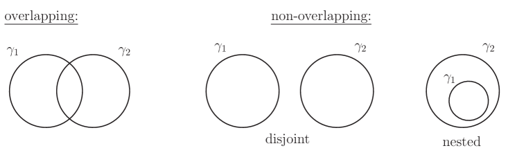
Figure 2: Types of subgraphs

For a given graph $\Gamma$, a $1PI$ subgraph $\gamma\subset\Gamma$ may be superficially divergent, i.e. its superficial degree of divergence $\delta(\gamma)$ satisfies $\delta(\gamma)\geq 0$: this subgraph is then called a renormalization part of $\Gamma$.

For a given graph $\Gamma$, we may have different types of subgraphs $\gamma$: There may be overlapping graphs and non-overlapping ones, and among the latter we can distinguish the disjunct and the nested ones. This situation is best summarized [16] by Fig. 2.

More precisely, consider two subgraphs $\gamma_{1}$ and $\gamma_{2}$. If $\gamma_{1}$ is completely included in $\gamma_{2}$ as a subgraph ($\gamma_{1}\subset\gamma_{2}$), then $\gamma_{1}$ is said to be nested in $\gamma_{2}$ and $\gamma_{2}$ is called a nested graph. The subgraphs $\gamma_{1}$ and $\gamma_{2}$ are said to be disjunct $(\gamma_{1}\cap\gamma_{2}=\emptyset)$ if they have no line or vertex in common. The subgraphs $\gamma_{1}$ and $\gamma_{2}$ are referred to as non-overlapping if one of the following conditions is satisfied:

$$\gamma_{1} \subset\gamma_{2}\,,\quad\gamma_{2}\subset\gamma_{1}\,,\quad\gamma_{1}\cap\gamma_{2}=\emptyset\,.$$ (21)

Otherwise these subgraphs are called overlapping. In the latter case, the diagrams have some common internal lines and vertices, and their union is referred to as the overlapping diagram; the divergence resulting from such a diagram is called the overlapping divergence. Due to their very nature, the elimination of such divergences requires two different subtractions. This fact represents a serious problem (the infamous “overlap problem”) for a recursive proof of the renormalizability for a given theory if one uses a method (like Dyson’s original counterterm method) in which all subgraphs, including the overlapping ones, have to be taken into account. As we will see in Section 2.5, the BPHZ method (and more precisely the forest formula) circumvents these problems since it only requires to deal with non-overlapping subgraphs.

For a graph $\Gamma$, one can introduce different sets of subgraphs $\gamma\subset\Gamma$ where $\gamma$ may be the full graph $\Gamma$ or the empty graph $\emptyset$. These sets are generically referred to as forests and in our overview we do not discuss the classification of forests.

The unrenormalized integrand corresponding to the graph $\Gamma$ can be decomposed with respect to the one of a subgraph $\gamma\subset\Gamma$ according to

$$I_{\Gamma}(p,k)=I_{\Gamma/\gamma}I_{\gamma}(p^{\gamma},k^{\gamma})\,.$$ (22)

Here the so-called reduced diagram $\Gamma/\gamma$ is obtained from $\Gamma$ by contracting $\gamma$ to a point. Moreover, the internal and external momenta $k^{\gamma}$ and $p^{\gamma}$ of the subgraph $\gamma$ have to be chosen to be consistent with the ones parameterizing the graph $\Gamma$ and with the energy-momentum conservation at the external vertices of the subgraph. This choice can be formalized by the introduction of the so-called substitution operator $S_{\gamma}$ [4] whose action is best illustrated by considering the example of the subgraph $\gamma_{1}$ of the sunrise graph $\Gamma$, as we will do in the following subsection.

2.4 Example: subgraphs of the sunrise graph

As an example of a graph with overlapping divergences we consider the case of the sunrise graph in $\phi^{4}$-theory which is depicted in Fig. 3.

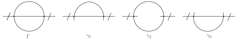
Figure 3: Sunrise graph $\Gamma$ and subgraphs $\gamma_{i}$

$\Gamma$ represents the full sunrise graph with $\delta(\Gamma)=2$, whereas the $\gamma_{i}$ are the non-trivial subgraphs all of which satisfy $\delta(\gamma_{i})=0$.

Let us make [16, 22] the assignment of momenta for the sunrise graph shown in Fig. 4.

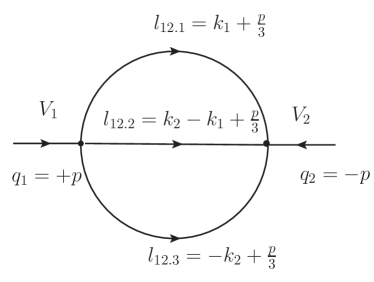
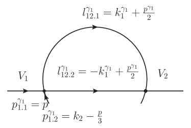
Figure 4: Sunrise graph $\Gamma$ and subgraph $\gamma_{1}$ with momenta

Here, $l_{12.i}$ with $i\in\{1,2,3\}$ denotes the different momenta flowing from vertex $V_{1}$ to vertex $V_{2}$. For the subgraph $\gamma_{1}$ one chooses the assignment of momenta shown in Fig. 4 (the external momenta $p_{1.1}^{\gamma_{1}}$ and $p_{1.2}^{\gamma_{1}}$ at the vertex $V_{1}$ of the subgraph $\gamma_{1}$ being determined by the corresponding momenta of the graph $\Gamma$). The values of the internal momenta of the subgraph $\gamma_{1}$ are determined by looking at vertex $V_{1}$ and by comparing with the momenta in graph $\Gamma$:

$$p^{\gamma_{1}}\equiv p_{1.1}^{\gamma_{1}}+p_{1.2}^{\gamma_{1}}\stackrel{{\scriptstyle!}}{{=}}p+\left(k_{2}-\frac{p}{3}\right)=k_{2}+\frac{2p}{3}\,,$$

$$k_{1}^{\gamma_{1}}+\frac{p^{\gamma_{1}}}{2}\stackrel{{\scriptstyle!}}{{=}}k_{1}+\frac{p}{3}\,.$$ (23)

By combining these two relations we get

$$k_{1}^{\gamma_{1}}+\frac{1}{2}\left(k_{2}+\frac{2p}{3}\right)\stackrel{{\scriptstyle!}}{{=}}k_{1}+\frac{p}{3}\,,$$ (24)

i.e. in summary

$$p^{\gamma_{1}} =k_{2}+\frac{2p}{3}\,,\qquad k_{1}^{\gamma_{1}}=k_{1}-\frac{k_{2}}{2}\,.$$ (25)

We note that this assignment of momenta is consistent with the one of the “horizontal” line of the graphs $\Gamma$ and $\gamma_{1}$:

$$\frac{p^{\gamma_{1}}}{2}-k^{\gamma_{1}}_{1}=\frac{k_{2}}{2}+\frac{p}{3}-k_{1}+\frac{k_{2}}{2}=k_{2}-k_{1}+\frac{p}{3}.$$ (26)

This illustrates how the assignment of momenta (or equivalently the action of the substitution operator) works. We note that the reduced diagram ${\Gamma/\gamma_{1}}$ is the tadpole graph with loop momentum $-k_{2}+\frac{p}{3}$ so that the corresponding integrand is given by $I_{\Gamma/\gamma_{1}}=\tilde{\Delta}(-k_{2}+\frac{p}{3})$ where $\tilde{\Delta}$ denotes the momentum space propagator (4). For later reference, we spell out the analog of $k_{1}^{\gamma_{1}}$ in (25) for the subgraphs $\gamma_{2}$ and $\gamma_{3}$, respectively:

$$k_{2}^{\gamma_{2}}=\frac{1}{2}(k_{1}+k_{2})\,,\qquad k_{3}^{\gamma_{3}}=-k_{2}+\frac{1}{2}\,k_{1}\,.$$ (27)

2.5 Subtraction of subdivergences: Forest formula

Suppose the Feynman graph $\Gamma$ contains one or several renormalization parts $\gamma$ with $\gamma\neq\Gamma$. To simplify the notation, the Taylor expansion operator for the graph $\gamma$, which is defined as in equation (10) and which picks out a potentially divergent part of $\gamma$, is written for short as $t_{\gamma}$.

A finite Feynman integral can be obtained for the graph $\Gamma$ by subtracting all divergences of the integral from its integrand $I_{\Gamma}$: this is achieved by applying the subtraction operator $1-t_{\gamma}$ for all renormalization parts $\gamma$, i.e. Bogoliubov’s $R$-operation (16) now acts on $I_{\Gamma}$ according to

$$\framebox{\mbox{$\ R_{\Gamma}I_{\Gamma}\equiv(1-t_{\Gamma})\Big{(}\prod_{\gamma\in{\cal F}}(1-t_{\gamma})\Big{)}I_{\Gamma}\ $}}\,.$$ (28)

Here, the subtraction $1-t_{\Gamma}$ allows to eliminate an overall divergence from the graph $\Gamma$: if none is present, the action of $t_{\Gamma}$ gives zero. The set (“forest”) $\mathcal{F}$ consists of all renormalization parts $\gamma$ with $\gamma\neq\Gamma$ and it is understood that the subtractions are performed from inside out, i.e. for nested subgraphs $\gamma\subset\gamma^{\prime}$, the subtraction $1-t_{\gamma}$ is performed before $1-t_{{\gamma}^{\prime}}$. The procedure (28) is an algorithmic method which can always be applied to eliminate potentially divergent contributions from a given graph and to obtain thereby absolutely convergent Feynman integrals (Weinberg’s power counting theorem).

An important result established on general grounds by Bergère and Zuber [34] is that overlapping subgraphs can be discarded from formula (28). More precisely, suppose $\gamma_{1}$ and $\gamma_{2}$ are overlapping renormalization parts of $\Gamma$; then, one has

$$(1-t_{{\gamma}_{12}})t_{\gamma_{1}}t_{\gamma_{2}}=0\,,$$ (29)

where ${\gamma}_{12}$ is a suitable renormalization part of $\Gamma$ which contains both $\gamma_{1}$ and $\gamma_{2}$ as subgraphs. More generally, relation (29) holds if the product $t_{\gamma_{1}}t_{\gamma_{2}}$ involves more factors corresponding to overlapping renormalization parts. In the approach to renormalization based on counterterms, the result (29) means that the overlapping divergences (which can lead to non-local counterterms) are always eliminated by lower order counterterms (see references [28, 29] for some explicit calculations) and therefore do not require the introduction of specific counterterms (which would correspond to a non-vanishing subtraction $(1-t_{{\gamma}_{12}})t_{\gamma_{1}}t_{\gamma_{2}}$).

As a simple example, assume that $\Gamma=\gamma_{1}\cup\gamma_{2}$ where $\gamma_{1}$ and $\gamma_{2}$ are overlapping subgraphs of the divergent graph $\Gamma$. Then, relation (29) yields $(1-t_{\Gamma})t_{{\gamma}_{1}}t_{{\gamma}_{2}}=0$ so that expression (28) can be rewritten as

$$R_{\Gamma}I_{\Gamma} \equiv(1-t_{\Gamma})(1-t_{\gamma_{1}})(1-t_{\gamma_{2}})I_{\Gamma}=(1-t_{\Gamma})(1-t_{\gamma_{1}}-t_{\gamma_{2}})I_{\Gamma}\,.$$ (30)

Quite generally, if we substitute equation (29) and its generalizations involving more factors $t_{\gamma_{i}}$ (corresponding to overlapping subgraphs $\gamma_{i}$) into relation (28), we conclude that

$$\framebox{\mbox{$\ R_{\Gamma}I_{\Gamma}=(1-t_{\Gamma})\sum_{\alpha}\Big{(}\prod_{\gamma\in{\cal F}_{\alpha}}(-t_{\gamma})\Big{)}I_{\Gamma}\ $}}\,.$$ (31)

Here, the index $\alpha\in\{0,1,\dots\}$ labels all sets (forests) ${\cal F}_{\alpha}$ of renormalization parts $\gamma\subset\Gamma,\,\gamma\neq\Gamma$, each of these sets containing only non-overlapping subgraphs. Moreover, one also takes into account the empty forest ${\cal F}_{0}\equiv\{\emptyset\}$ given by the empty set for which one sets $-t_{\emptyset}\equiv 1$. Relation (31) is referred to as Zimmermann’s forest formula (for Bogoliubov’s $R$-operation).

In example (30) one has ${\cal F}_{0}=\{\emptyset\},\,{\cal F}_{1}=\{\gamma_{1}\},\,{\cal F}_{2}=\{\gamma_{2}\}$. Similarly for the sunrise graph in $\phi^{4}$-theory, we have ${\cal F}_{0}=\{\emptyset\}$ and ${\cal F}_{i}=\{\gamma_{i}\}$ for $i=1,2,3$ so that the forest formula for the sunrise graph reads

$$R_{\Gamma}I_{\Gamma}=(1-t_{\Gamma})\;\Big{(}1+\sum_{i=1}^{3}(-t_{\gamma_{i}})\Big{)}I_{\Gamma}\,.$$ (32)

The subtraction operator $t_{\gamma_{i}}$ only affects the subgraph $\gamma_{i}$ of $\Gamma$ and $t_{\gamma_{i}}I_{\gamma_{i}}$ amounts to picking out the divergent part of $\gamma_{i}$ (i.e. generating the local counterterm which allows to subtract the divergence due to $\gamma_{i}$). Thus, the effect of $t_{\gamma_{i}}$ on $I_{\Gamma}$ is to contract the subgraph $\gamma_{i}$ to a point (thereby yielding the reduced graph $\Gamma/\gamma_{i}$) and to pick out the divergent part of $\gamma_{i}$:

$$t_{\gamma_{i}}I_{\Gamma}=I_{\Gamma/\gamma_{i}}\;t_{\gamma_{i}}I_{\gamma_{i}}\,.$$ (33)

Henceforth, the forest formula for the sunrise graph reads [22]

$$R_{\Gamma}I_{\Gamma} =(1-t_{\Gamma})\;\Big{(}I_{\Gamma}-\sum_{i=1}^{3}I_{\Gamma/\gamma_{i}}\,t_{\gamma_{i}}I_{\gamma_{i}}\Big{)}$$

$$=I_{\Gamma}-t_{\Gamma}I_{\Gamma}-\sum_{i=1}^{3}I_{\Gamma/\gamma_{i}}\,t_{\gamma_{i}}I_{\gamma_{i}}+\sum_{i=1}^{3}t_{\Gamma}\,\big{(}I_{\Gamma/\gamma_{i}}\,t_{\gamma_{i}}I_{\gamma_{i}}\big{)}\,,$$ (34)

where the implementation of the substitution operator $S_{\gamma_{i}}$ for the subgraphs $\gamma_{i}$ (discussed in Subsections 2.3 and 2.4) is self-understood.

To conclude, we come back to the general case and introduce the subtraction operator $\bar{R}_{\Gamma}$ for the subdivergences of the graph $\Gamma$ by

$$R_{\Gamma}I_{\Gamma}\equiv(1-t_{\Gamma})\bar{R}_{\Gamma}I_{\Gamma}\,.$$ (35)

According to Eqn. (31), the forest formula for $\bar{R}_{\Gamma}$ then reads

$$\framebox{\mbox{$\ \bar{R}_{\Gamma}I_{\Gamma}=\sum_{\alpha}\Big{(}\prod_{\gamma\in{\cal F}_{\alpha}}(-t_{\gamma})\Big{)}I_{\Gamma}\ $}}\,,$$ (36)

where $\alpha\in\{0,1,\dots\}$ labels all forests ${\cal F}_{\alpha}$ which contain only non-overlapping subgraphs.

2.6 Recursion relation for Bogoliubov’s operator

It can be shown [4] that the operator $\bar{R}_{\Gamma}$ satisfies the BPHZ recursion relation

$$\framebox{\mbox{$\ \bar{R}_{\Gamma}I_{\Gamma}=\sum_{\Psi}\Big{(}\prod_{\gamma\in{\Psi}}(-t_{\gamma})\bar{R}_{\gamma}\Big{)}I_{\Gamma}\ $}}\,,$$ (37)

or, equivalently

$$\bar{R}_{\Gamma}I_{\Gamma} =\sum_{\Psi}I_{\Gamma/\Psi}\prod_{\gamma\in{\Psi}}(-t_{\gamma})\bar{R}_{\gamma}I_{\gamma}\,,$$ (38)

where $\Psi$ labels all possible sets of the form

$$\Psi=\{\gamma\,/\,\gamma=\mbox{disjoint renormalization part of $\Gamma$}\}\,,$$

including the case $\Psi=\{\emptyset\}$. Before explaining the passage from (37) to (38), we emphasize two points. The recursion relation determines the operator $\bar{R}_{\Gamma}$ recursively in terms of the operators $\bar{R}_{\gamma}$ corresponding to lower order graphs $\gamma$. The recursion relation only involves disjoint subgraphs while the forest formula refers to non-overlapping subgraphs, i.e. to both disjoint and nested subgraphs.

Let us now explain the expression on the right hand side of Eqn. (38). For a set $\{\gamma_{1},\ldots,\gamma_{n}\}$ of mutually disjoint renormalization parts of the graph $\Gamma$, one defines the reduced diagram ${\Gamma/\{\gamma_{1},\ldots,\gamma_{n}\}}$ by contracting each $\gamma_{i}$ to a point. For disjoint subgraphs $\gamma_{1},\gamma_{2}$ of $\Gamma$, the order of $t_{\gamma_{1}}$ and $t_{\gamma_{2}}$ does not matter and we have

$$t_{\gamma_{1}}t_{\gamma_{2}}I_{\Gamma}=I_{\Gamma/\{\gamma_{1},\gamma_{2}\}}(t_{\gamma_{1}}I_{\gamma_{1}})(t_{\gamma_{2}}I_{\gamma_{2}})\,,$$ (39)

and

$$\Big{(}(t_{\gamma_{1}}\bar{R}_{\gamma_{1}})(t_{\gamma_{2}}\bar{R}_{\gamma_{2}})\Big{)}I_{\Gamma}=I_{\Gamma/\{\gamma_{1},\gamma_{2}\}}(t_{\gamma_{1}}\bar{R}_{\gamma_{1}}I_{\gamma_{1}})(t_{\gamma_{2}}\bar{R}_{\gamma_{2}}I_{\gamma_{2}})\,,$$ (40)

which explains the equivalence between Equations (37) and (38). By contrast, for nested subgraphs $\gamma_{1}\subset\gamma_{2}$, we have to apply $t_{\gamma_{1}}$ first and Eqn. (33) yields

$$t_{\gamma_{2}}t_{\gamma_{1}}I_{\Gamma}=I_{\Gamma/\gamma_{2}}\,t_{\gamma_{2}}\Big{(}I_{\gamma_{2}/\gamma_{1}}(t_{\gamma_{1}}I_{\gamma_{1}})\Big{)}\,.$$ (41)

The fact that the forest formula (36) solves the recursion relation (37) can easily be checked for the example (30): in this case, $\Psi=\{\emptyset\}$ or $\Psi=\{\gamma_{1}\}$ or $\Psi=\{\gamma_{2}\}$, hence (38) states that

$$\bar{R}_{\Gamma}I_{\Gamma}=I_{\Gamma}-I_{\Gamma/\gamma_{1}}t_{\gamma_{1}}(\bar{R}_{\gamma_{1}}I_{\gamma_{1}})-I_{\Gamma/\gamma_{2}}t_{\gamma_{2}}(\bar{R}_{\gamma_{2}}I_{\gamma_{2}})\,.$$ (42)

Since $\gamma_{1}$ does not contain any subdivergences, the action of the operator $\bar{R}_{\gamma_{1}}$ (which eliminates all subdivergences from the graph ${\gamma_{1}}$) on $I_{\gamma_{1}}$ is trivial, i.e. $\bar{R}_{\gamma_{1}}I_{\gamma_{1}}=I_{\gamma_{1}}$ (and similarly $\bar{R}_{\gamma_{2}}I_{\gamma_{2}}=I_{\gamma_{2}}$), hence

$$\bar{R}_{\Gamma}I_{\Gamma}=I_{\Gamma}-I_{\Gamma/\gamma_{1}}\,t_{\gamma_{1}}I_{\gamma_{1}}-I_{\Gamma/\gamma_{2}}\,t_{\gamma_{2}}I_{\gamma_{2}}=(1-t_{\gamma_{1}}-t_{\gamma_{2}})I_{\Gamma}\,,$$ (43)

so that

$$R_{\Gamma}I_{\Gamma}\equiv(1-t_{\Gamma})\bar{R}_{\Gamma}I_{\Gamma}=(1-t_{\Gamma})(1-t_{\gamma_{1}}-t_{\gamma_{2}})I_{\Gamma}\,,$$ (44)

i.e. the forest formula (30) for the example under consideration.

2.7 Example: Renormalization of the sunrise graph

The sunrise graph involves two interaction vertices, i.e. a factor ${\lambda}^{2}$. The unrenormalized sunrise graph is described by the integral

$$J_{\Gamma}(p) \equiv\int d^{4}k_{1}\int d^{4}k_{2}\,I_{\Gamma}(p,k_{1},k_{2})\,,$$ (45)

where the integrand is a product of propagators (4) – see Fig. 4 :

$$I_{\Gamma}(p,k_{1},k_{2}) \equiv\tilde{\Delta}\big{(}\frac{p}{3}+k_{1}\big{)}\,\tilde{\Delta}\big{(}\frac{p}{3}+k_{2}-k_{1}\big{)}\,\tilde{\Delta}\big{(}\frac{p}{3}-k_{2}\big{)}\,.$$ (46)

(In expression (45), we suppressed the numerical prefactor involving $\lambda^{2}$.) The renormalized sunrise graph is now given by

$$J^{{\rm finite}}_{\Gamma}(p) =\int d^{4}k_{1}\int d^{4}k_{2}\,\big{(}R_{\Gamma}I_{\Gamma}\big{)}(p,k_{1},k_{2})\,,\quad$$

$$\textrm{with}\quad R_{\Gamma}I_{\Gamma} \equiv(1-t_{\Gamma})\,\bar{R}_{\Gamma}I_{\Gamma}=(1-t_{p}^{2})\,\bar{R}_{\Gamma}I_{\Gamma}\,,$$ (47)

where $\bar{R}_{\Gamma}I_{\Gamma}$ is determined by the forest formula for the sunrise graph, i.e. Eqn. (2.5):

$$\big{(}\bar{R}_{\Gamma}I_{\Gamma}\big{)}(p,k_{1},k_{2}) =\tilde{\Delta}\big{(}\frac{p}{3}+k_{1}\big{)}\,\tilde{\Delta}\big{(}\frac{p}{3}+\!k_{2}\!-\!k_{1}\big{)}\,\tilde{\Delta}\big{(}\frac{p}{3}-k_{2}\big{)}-\tilde{\Delta}\big{(}\frac{p}{3}-k_{2}\big{)}\,\left[\tilde{\Delta}\big{(}k_{1}-\frac{k_{2}}{2}\big{)}\right]^{2}$$

$$\quad-\tilde{\Delta}\big{(}\frac{p}{3}+\!k_{2}\!-\!k_{1}\big{)}\,\left[\tilde{\Delta}\big{(}\frac{k_{1}}{2}+\frac{k_{2}}{2}\big{)}\right]^{2}-\tilde{\Delta}(\frac{p}{3}+k_{1})\,\left[\tilde{\Delta}(k_{2}\!-\!\frac{k_{1}}{2})\right]^{2}.$$ (48)

To evaluate the integral $\int d^{4}k_{1}\int d^{4}k_{2}\,\big{(}\bar{R}_{\Gamma}I_{\Gamma}\big{)}(p,k_{1},k_{2})$, one substitutes Schwinger’s parametric representation for the propagators,

$$\tilde{\Delta}(q_{i})\equiv\frac{1}{q_{i}^{2}+m^{2}}=\int\limits_{0}^{\infty}d\alpha_{i}\,{\rm e}^{-\alpha_{i}(q_{i}^{2}+m^{2})}\,,$$ (49)

so that the integration over $\vec{k}\equiv(k_{1},k_{2})\in\mathds{R}^{8}$ yields integrals of Gaussian type,

$$\int d^{8}k\,{\rm e}^{-\langle\vec{k},A\vec{k}\,\rangle-\langle\vec{b},\vec{k}\,\rangle}={\rm e}^{\langle\vec{b},A^{-1}\vec{b}\,\rangle}\,\left(\frac{\pi}{\sqrt{{\rm det}\,A}}\right)^{4}\,.$$

Thus, one finds that

$$J^{{\rm finite}}_{\Gamma}(p) =\pi^{4}\int\limits_{0}^{\infty}d\alpha_{1}\int\limits_{0}^{\infty}d\alpha_{2}\int\limits_{0}^{\infty}d\alpha_{3}\,{\rm e}^{-(\alpha_{1}+\alpha_{2}+\alpha_{3})m^{2}}(1-t_{p}^{2})\,\Bigg{\{}\frac{{\rm e}^{-\beta\,p^{2}}}{(\alpha_{1}\alpha_{2}+\alpha_{2}\alpha_{3}+\alpha_{1}\alpha_{3})^{2}}$$

$$\hskip 110.96556pt-\frac{1}{\alpha_{1}^{2}(\alpha_{2}+\alpha_{3})^{2}}-\frac{1}{\alpha_{2}^{2}(\alpha_{1}+\alpha_{3})^{2}}-\frac{1}{\alpha_{3}^{2}(\alpha_{1}+\alpha_{2})^{2}}\Bigg{\}}\,,$$ (50)

where $\beta\equiv\frac{\alpha_{1}\alpha_{2}\alpha_{3}}{\alpha_{1}\alpha_{2}+\alpha_{2}\alpha_{3}+\alpha_{1}\alpha_{3}}$. Finally, from

$$-\frac{1}{2}\,p^{\mu}p^{\nu}\,\left.\frac{\partial^{2}{\rm e}^{-\beta\,p^{2}}}{\partial p^{\mu}\partial p^{\nu}}\right|_{p=0}=\,\beta\,p^{2}\,,$$

we conclude that the renormalized sunrise graph is given by

$$J^{{\rm finite}}_{\Gamma}(p) =\pi^{4}\,\int\limits_{0}^{\infty}d\alpha_{1}\int\limits_{0}^{\infty}d\alpha_{2}\int\limits_{0}^{\infty}d\alpha_{3}\,\frac{{\rm e}^{-(\alpha_{1}+\alpha_{2}+\alpha_{3})m^{2}}}{(\alpha_{1}\alpha_{2}+\alpha_{2}\alpha_{3}+\alpha_{1}\alpha_{3})^{2}}\left\{{\rm e}^{-\beta\,p^{2}}-(1-\beta p^{2})\right\}\,.$$ (51)

2.8 Relationship to additive (and multiplicative) renormalization

Let us investigate how the subtractions performed for the sunrise graph $\Gamma$ affect the initial Lagrangian of the $\phi^{4}$-theory [32]. For the quadratically divergent graph $\Gamma$ we expand the integrand $I\equiv I_{\Gamma}$ in a Taylor series with respect to the external momentum $p$ around $p=0$:

$$I(p,k_{1},k_{2}) =\big{(}t_{p}^{2}I\big{)}(p,k_{1},k_{2})+R(p,k_{1},k_{2})\,.$$ (52)

Here, $t_{p}^{2}$ denotes as before the Taylor series expansion operator up to order $2$ in $p$, and the remainder term $R$ decays strong enough with respect to $k_{1}$ and $k_{2}$ that it yields a finite contribution to the Feynman integral $\int d^{4}k_{1}\int d^{4}k_{1}\,I(p,k_{1},k_{2})$. By explicitly spelling out the terms of order $0,1$ and $2$ in $p^{\mu}$ which make up the expansion

$$\big{(}t_{p}^{2}I\big{)}(p,k_{1},k_{2})=t_{p}^{2}\Big{(}\tilde{\Delta}\big{(}\frac{p}{3}+k_{1}\big{)}\,\tilde{\Delta}\big{(}\frac{p}{3}+\!k_{2}\!-\!k_{1}\big{)}\,\tilde{\Delta}\big{(}\frac{p}{3}-k_{2}\big{)}\Big{)}\,,$$ (53)

one notes that these terms yield a quadratic, linear and logarithmic divergence in the Feynman integral, respectively. To handle these divergences, we introduce a cut-off $\Lambda>0$ in momentum space and a smooth test function $(k_{1},k_{2})\mapsto f(k_{1},k_{2})$ of compact support (i.e. $f\in{\cal D}(\mathds{R}^{8})$) satisfying $f(0,0)=1$. To regularize the integrand $I$, we now smear out with the function $f_{\Lambda}$ defined by

$$f_{\Lambda}(k_{1},k_{2})\equiv f\Big{(}\frac{k_{1}}{\Lambda},\frac{k_{2}}{\Lambda}\Big{)}\,,$$ (54)

which tends to $1$ as the cut-off $\Lambda$ goes to infinity, i.e. we consider the regularized integral

$$J_{\Lambda}(p) \equiv\int d^{4}k_{1}\int d^{4}k_{1}\,f_{\Lambda}(k_{1},k_{2})\,I(p,k_{1},k_{2})$$

$$=a(\Lambda)+b_{\mu}(\Lambda)\,p^{\mu}+c_{\mu\nu}(\Lambda)\,p^{\mu}p^{\nu}+R(p,\Lambda)\,.$$ (55)

For $\Lambda\to\infty$, we have $a(\Lambda)\propto\Lambda^{2},\,b_{\mu}(\Lambda)\propto\Lambda$ and $c_{\mu\nu}(\Lambda)\propto\ln\Lambda$, while $R(p,\Lambda)$ yields a regular function $R(p)$.

The freedom in the choice of the test function $f$ can be exploited to achieve $b_{\mu}=0$ and $c_{\mu\nu}(\Lambda)=c(\Lambda)\delta_{\mu\nu}$. The subtraction of the divergent part $t_{p}^{2}I$ from the integrand $I$, which was considered in the BPHZ approach, therefore amounts to adding to the momentum space action the counterterm

$$\frac{1}{2}\int\frac{d^{4}p}{(2\pi)^{4}}\,\big{(}a+c\,p^{2}\big{)}\tilde{\phi}^{2}=\frac{1}{2}\int d^{4}x\,\Big{(}c\,\partial^{\mu}\phi\partial_{\mu}\phi+a\phi^{2}\Big{)}\,,$$ (56)

i.e. we have a local counterterm for the (quadratic part of the) Lagrangian which has the same form as the initial action (“additive renormalization”).

Up to the considered order of perturbation theory, the (quadratic part of the) redefined Lagrangian thus has the form

$${\cal L}_{\rm ren}=\frac{1}{2}\,\big{(}1+c(\Lambda)\big{)}\partial^{\mu}\phi\partial_{\mu}\phi+\frac{1}{2}\,\big{(}m^{2}+a(\Lambda)\big{)}\phi^{2}\,.$$ (57)

With

$$Z(\Lambda)\equiv 1+c(\Lambda)\,,\quad\phi_{\rm ren}\equiv\sqrt{Z(\Lambda)}\,\phi\,,\quad m_{\rm ren}^{2}\equiv\big{(}m^{2}+a(\Lambda)\big{)}\,Z(\Lambda)^{-1}\,,$$ (58)

we have (“multiplicative renormalization”)

$${\cal L}_{\rm ren}=\frac{1}{2}\,\partial^{\mu}\phi_{\rm ren}\partial_{\mu}\phi_{\rm ren}+\frac{1}{2}\,m_{\rm ren}^{2}\phi_{\rm ren}^{2}\,.$$ (59)

After the renormalizations have been performed, it is still possible to add finite ($\Lambda$-independent) terms to $a(\Lambda)$ and $c(\Lambda)$: these finite renormalizations have been encountered in Subsection 2.2 as the ambiguity of extracting the finite part $J_{\Gamma}^{{\rm finite}}(p)$ from the quadratically divergent integral $J_{\Gamma}(p)$.

As we noted in Subsection 2.2, the subtraction (12) for the logarithmically divergent fish diagram (8) leads to the addition of a local counterterm of the form $d(\Lambda)\phi^{4}$ to the Lagrangian, i.e. a contribution of the same form as the interaction term $\frac{\lambda}{4!}\,\phi^{4}$ which is present in the initial Lagrangian.

For the comparison with (and relationship to) other approaches to renormalization, we refer to the work [36, 37].

2.9 Locality of subtractions and renormalizability

The application of the forest formula to each graph $\Gamma$ allows to render all Feynman integrals convergent. The second step of the BPHZ renormalization procedure consists of showing that the performed subtractions are equivalent to the addition of local counterterms to the Lagrangian. The consideration of the forest formula is not judicious for establishing this equivalence since it does not explicitly refer to the different orders of perturbation theory [28]. As discussed in Subsection 2.6, the forest formula solves the BPHZ recursion relation, and the latter relates the subtractions performed at different orders of perturbation theory so that this relation can be used to establish locality of the renormalization process. In fact, whatever the graph or subgraph $\Gamma$ to which the recursion relation (37) or (38) is applied to, it relates $\bar{R}_{\Gamma}$ to $\bar{R}_{\gamma}$ for subgraphs $\gamma$ and thereby different orders of perturbation theory. Accordingly, if one can show that the field theoretic model under consideration is renormalizable at one-loop order (i.e. the BPHZ subtraction for divergent one-loop graphs can be implemented by the addition of a local counterterm), then the locality of the counterterms at two-loop order follows from the recursion relation for the two-loop subgraphs $\Gamma(2)$ of a given graph $\Gamma$:

$$\bar{R}_{\Gamma(2)}I_{\Gamma(2)} =\sum_{\Psi(1)}I_{\Gamma(2)/\Psi(1)}\prod_{\gamma(1)\in{\Psi(1)}}\big{(}-t_{\gamma(1)}\big{)}\,I_{\gamma(1)}\,,$$ (60)

where $\Psi(1)$ labels the sets of disjoint one-loop renormalization parts and where we used the fact that $\bar{R}_{\gamma(1)}I_{\gamma(1)}=I_{\gamma(1)}$. By virtue of (60) all one-loop subdivergences are eliminated in the two-loop subgraphs $\Gamma(2)$. By proceeding along the same lines for higher order subgraphs of $\Gamma$ and applying the operator $(1-t_{\Gamma})$ in the end to subtract a possible overall divergence of $\Gamma$, one establishes the locality of counterterms and thereby shows the equivalence of the BPHZ approach to renormalization to the method based on adding counterterms to the Lagrangian.

2.10 Case of massless fields ($s$-trick)

In view of the treatment of gauge fields we comment on the $\phi^{4}$-theory for a massless field. In this case, potential IR problems appear. For instance, the integral (8) corresponding to the fish diagram then reduces to $\int\!d^{4}k\,\frac{1}{k^{2}(p+k)^{2}}$: this integral admits an IR-divergence for $p=0$ which is precisely the value for which the BPHZ subtraction is performed. Thus, in the case of massless fields, the standard BPHZ subtraction scheme considered for discarding UV-divergences may introduce some artificial IR-singularities [18, 19, 20, 21, 15]. The remedy consists of making the subtraction either for a non-zero value of $p$ or for a non-zero value of the mass. Following Lowenstein et al. [18, 19, 20, 21, 15] one generally adopts the latter procedure for its simplicity. More precisely, one introduces a mass factor $M_{s}\equiv(1-s)M$, which involves an auxiliary mass $M$ and a real auxiliary variable $s$ (the “softness parameter”), in the effective Lagrangian and thereby in all internal propagators:

$$\frac{1}{k^{2}}\;\leadsto\;\frac{1}{k^{2}+M_{s}^{2}}\,,\qquad{\rm with}\ \;M_{s}=(1-s)M\,.$$ (61)

Then, one applies the Taylor expansion operator $t_{p,s}^{\delta(\Gamma)}$ around both $p=0$ and $s=0$, while setting $s=1$ at the end of the calculation (the whole procedure being sometimes referred to as $s$-trick). The possible IR-divergences due to the vanishing mass of the physical fields (external zero mass lines of Feynman graphs) have to be dealt with appropriately.

Thus, for a logarithmically divergent integral like $J_{\Gamma}(p)=\int\!d^{4}k\,\frac{1}{k^{2}(p+k)^{2}}\equiv\int\!d^{4}k\,I_{\Gamma}(p,k)$, the BPHZL subtraction amounts to considering the following expression (according to Eqns. (9),(11) and the previous arguments)

$$J_{\Gamma}^{{\rm finite}}(p) \equiv\lim_{s\to 1}\int\!d^{4}k\,\left[1-t_{p,s}^{0}\right]\,I_{\Gamma}(p,k,s)=\lim_{s\to 1}\int\!d^{4}k\,\left[I_{\Gamma}(p,k,s)-I_{\Gamma}(0,k,0)\right]$$

$$=\int\!d^{4}k\,\left(\frac{1}{k^{2}(p+k)^{2}}-\frac{1}{(k^{2}+M^{2})^{2}}\right)\,.$$ (62)

Accordingly, the subtraction term involves a mass so that it is not IR-divergent despite the fact that it involves a vanishing external momentum.

After substituting Schwinger’s parametrization of the propagators into the integral (62) and performing the resulting Gaussian integrals over the four vector $k$ (see for instance appendix of reference [38]), one obtains the expression

$$\frac{1}{\pi^{2}}\,J_{\Gamma}^{{\rm finite}}(p) =\int_{0}^{\infty}\frac{d\lambda}{\lambda}\,\bigg{\{}\int_{0}^{1}\,d\xi\,{{\rm e}}^{-\lambda\xi(1-\xi)p^{2}}-{{\rm e}}^{-\lambda M^{2}}\bigg{\}}\,,$$ (63)

The original UV-divergence of $\Gamma$ now manifests itself by a problematic behavior of the two $\lambda$-integrals for small values of the parameter $\lambda$. These integrals can be regularized [29] by multiplying the integrands by an exponential cut-off factor ${{\rm e}}^{-\varepsilon/\lambda}$ and considering the limit $\varepsilon\to 0$ for the resulting integral. Proceeding along these lines one finds

$$\frac{1}{\pi^{2}}\,J_{\Gamma}^{{\rm finite}}(p) =\ln\left(\frac{M^{2}}{p^{2}}\right)+2\,,$$ (64)

i.e. a result which has the same form as the one obtained by expanding the BPHZ-renormalized fish diagram of the massive $\phi^{4}$-theory [5] for small values of the mass $m$:

$$J_{\Gamma}^{{\rm finite}}(p;m) \propto\sqrt{\frac{p^{2}+4m^{2}}{p^{2}}}\,\ln{\left[\frac{\sqrt{p^{2}+4m^{2}}-\sqrt{p^{2}}}{\sqrt{p^{2}+4m^{2}}+\sqrt{p^{2}}}\right]}+2\approx\ln\left(\frac{m^{2}}{p^{2}}\right)+2\,.$$ (65)

The $M$-dependent one-loop result (64) for the four-point function is absorbed by choosing an appropriate $M$-dependent coefficient $d$ (i.e. counterterm $d\,\phi^{4}$) which is adjusted in such a way that the Green functions satisfy normalization conditions that do not depend on the auxiliary mass $M$ [19]. Thereby, the final theory does not depend on the auxiliary mass $M$ and describes a well defined massless quantum field theory. For further details, e.g. a discussion of the BPHZL-renormalization of the sunrise graph within the massless $\phi^{4}$-theory, we refer to the work [19] (in particular its conclusion).

2.11 Assessment

Let us summarize once more the salient features of the BPHZ scheme [25]. Following Zimmermann [16], the subtractions providing convergent integrals are directly applied to the integrands, hence no regulator has to be considered. Accordingly, this procedure exhibits the fact that the properties of the resulting quantum theory do not depend on a regulator or on the way it is introduced. Moreover, general mathematical theorems based on simple properties of Taylor series ensure that finite integrals can be constructed from divergent ones without explicitly investigating each Feynman diagram and its divergences. The BPHZ scheme is quite useful for discussing different issues of quantum theory like the operator product expansion [16, 17]. Following Lowenstein et al. [18, 19, 20, 21, 15] the BPHZ approach can be adapted to tackle massless fields though the subtractions are somewhat more complex in this case, in particular in the presence of gauge symmetries, e.g. see Ref. [39].

3 Non-commutative $\phi^{4}$-theory

We are now ready to turn to the non-commutative case and, after discussing general properties of the modified BPHZ approach introduced in reference [1], we study its application to the sunrise graph of non-commutative $\phi^{4}$-theory.

3.1 UV/IR mixing problem (Infrared singularities)

Before considering the BPHZ approach to the UV/IR mixing problem, it is useful to recall briefly the origin and nature of this problem [40].

In non-commutative field theories, the star product leads to the presence of phase factors in various Feynman graphs. In particular, the non-planar one-loop $2$-point function (non-planar tadpole graph) which is given, up to a numerical factor, by

$$\Pi_{\text{n-pl}}(\tilde{p})=\int\limits_{\mathds{R}^{4}}d^{4}k\,\frac{\cos(k\tilde{p})}{k^{2}+m^{2}}\,,$$ (66)

involves a phase factor of the form $\cos(k\tilde{p})$ where $p$ denotes the external momentum. For large values of $k$, the rapid oscillations of the phase factor have a damping effect upon integration; thus, for any $\tilde{p}\neq 0$, the function (66) is finite by contrast to the corresponding planar diagram which does not contain a phase factor,

$$\Pi_{\text{pl}}=\int\limits_{\mathds{R}^{4}}d^{4}k\,\frac{1}{k^{2}+m^{2}}\,,$$ (67)

and which is quadratically UV-divergent. Accordingly, the phase factor can be viewed as a regularization brought about the non-commutativity of space-time [40], i.e. an idea which is reminiscent of the historical arguments which led Heisenberg and Snyder to consider non-commutative space-time to overcome the problem of UV-divergences in quantum field theory [41, 42, 43, 44, 45]. However, the UV-divergent diagram (67) is still present in the theory and in addition the integral (66) is singular for small values of the external momentum (IR-divergent) [40, 46], the leading singularity being $1/{\tilde{p}}^{\,2}$:

$$\Pi_{\text{n-pl}}(\tilde{p}) =\frac{1}{(4\pi)^{2}}\bigg{[}\frac{4}{\tilde{p}^{\,2}}+m^{2}\ln(m^{2}\tilde{p}^{\,2})\bigg{]}+\mathcal{O}(1)\qquad{\rm for}\ \;\tilde{p}\ll 1\,.$$ (68)

To have a better understanding of this expansion, it is useful to first recall the cut-off regularization of the integral (67). In this respect, one substitutes Schwinger’s parametrization $(k^{2}+m^{2})^{-1}=\int_{0}^{\infty}d\alpha\,{\rm e}^{-\alpha(k^{2}+m^{2})}$ into (67) and performs the Gaussian integration over $k$ in order to obtain

$$\Pi_{\text{pl}}=\int_{0}^{\infty}\frac{d\alpha}{\alpha^{2}}\,{\rm e}^{-\alpha m^{2}}\,.$$ (69)

The UV-divergence of (67) now amounts to the singular behaviour of (69) for small values of $\alpha$. The divergence structure of this expression can be exhibited by cutting off the $\alpha$-integral at a lower limit $1/\Lambda^{2}$ (where $\Lambda\gg 1$ represents a momentum cut-off), expanding the exponential and carrying out the integration of the first few terms [29], or equivalently by cutting off the integrand by the introduction of an exponential factor ${\rm e}^{-(\Lambda^{2}\alpha)^{-1}}$:

$$\Pi_{\text{pl}} =\lim_{\Lambda\to\infty}\left(\Pi_{\text{pl}}\right)_{\rm reg}(\Lambda)\,,\qquad{\rm with}\ \;\left(\Pi_{\text{pl}}\right)_{\rm reg}(\Lambda)\equiv\int_{0}^{\infty}\frac{d\alpha}{\alpha^{2}}\,{\rm e}^{-\alpha m^{2}}\,{\rm e}^{-(\Lambda^{2}\alpha)^{-1}}\,.$$ (70)

The final result reflecting the quadratic UV-divergence of $\Pi_{\text{pl}}$ (and involving a subleading logarithmic divergence) reads

$$\left(\Pi_{\text{pl}}\right)_{\rm reg}(\Lambda)=\frac{1}{(4\pi)^{2}}\bigg{[}\Lambda^{2}-m^{2}\ln\frac{\Lambda^{2}}{m^{2}}\bigg{]}+\mathcal{O}(1)\qquad{\rm for}\ \;\Lambda\gg 1\,.$$ (71)

Let us now come back to the integral (66): substitution of Schwinger’s parametrization into this integral yields

$$\Pi_{\text{n-pl}}(\tilde{p})=\int_{0}^{\infty}\frac{d\alpha}{\alpha^{2}}\,{\rm e}^{-\alpha m^{2}}\,{\rm e}^{-\frac{\tilde{p}^{\,2}}{4\alpha}}\,,$$ (72)

i.e. the same integral as (70) with ${\Lambda^{2}}$ replaced by $\frac{4}{\tilde{p}^{\,2}}$, whence the expansion (68) [40, 46].

The non-planar one-loop $4$-point function involves an integral of the form (6) which can be discussed along the same lines: it is a function of $\tilde{p}$ (and of $p$) which is UV-finite, but involves a logarithmic IR-singularity (divergence for $\tilde{p}\to 0$), the latter reflecting the logarithmic UV-divergence of the corresponding planar diagram [29],

$$J_{\text{pl}}(p)=\lim_{\Lambda\to\infty}\left(J_{\text{pl}}\right)_{\rm reg}(p,\Lambda)\,,\quad{\rm with}\ \left(J_{\text{pl}}\right)_{\rm reg}(0,\Lambda)=\pi^{2}\bigg{[}\ln\frac{\Lambda^{2}}{m^{2}}-1\bigg{]}+\mathcal{O}(\frac{1}{\Lambda^{2}})\quad{\rm for}\ \;\Lambda\gg 1\,.$$

3.2 Modified BPHZ subtractions

As discussed in the previous subsection, the non-planar one-loop $n$-point function is UV-finite, but suffers from an IR-singularity which is tied to the UV-divergence of the corresponding planar diagram. Thus, for these non-planar graphs, our modified BPHZ subtraction amounts to an IR-subtraction rather than a UV-subtraction. When applying this subtraction to an integrand $I(p,\tilde{p},k)$, it is important to consider $p$ and $\tilde{p}$ as independent variables and to subtract the Taylor series expansion around $p=0$ (rather than $\tilde{p}=0$ which represents a divergence of the diagram):

$$I(p,\tilde{p},k)=I(0,\tilde{p},k)+p^{\mu}\,\frac{\partial I}{\partial p^{\mu}}(0,\tilde{p},k)+\dots\,.$$ (73)

For the subtracted non-planar one-loop $2$-point function, we get a vanishing result (as one also does for the planar, UV-divergent diagram by virtue of the standard BPHZ subtraction scheme, see Eqn. (19). For the subtracted non-planar one-loop $4$-point function (7), one obtains a result which is regular in $\tilde{p}$ [1]:

$$J^{{\rm finite}}(p) =-\pi^{2}\sqrt{1+\frac{4m^{2}}{p^{2}}}\,\ln{\left[\frac{\sqrt{p^{2}+4m^{2}}+\sqrt{p^{2}}}{\sqrt{p^{2}+4m^{2}}-\sqrt{p^{2}}}\right]}+2\pi^{2}+\mathcal{O}(\tilde{p}^{2})\,.$$ (74)

Finite renormalizations

Concerning the UV-divergent planar diagrams, we note that the cut-off regularization exhibits the UV-divergence as well as its degree (power of $\Lambda$), the latter determining also the degree of the polynomial in $p$ which is considered for the standard BPHZ subtraction, see equation (9). As discussed in Subsection 2.2 (see Eqn. (17)), the ambiguity involved in the standard BPHZ subtraction (corresponding to a finite renormalization) is a polynomial in $p$ whose order is the superficial degree of UV-divergence of the diagram under consideration.

A non-planar diagram and the regularized version of the corresponding planar diagram have the same form up to the replacement $\Lambda^{2}\leadsto 4/{\tilde{p}}^{\,2}$ – compare for instance equations (70) and (72). Hence one expects that the ambiguity involved in the modified BPHZ subtraction amounts to a polynomial in $1/\tilde{p}^{\,2}$ whose degree is determined by the degree of the IR-singularity of the non-planar graph. To confirm this expectation, we consider the expansion (73) for the modified BPHZ subtraction. The ambiguity is a polynomial in $p$ (with coefficients depending on the parameter $\tilde{p}^{\,2}$ which is considered as an independent variable), the degree of this polynomial coinciding with the degree of the IR-singularity of the non-planar graph. All coefficients of this polynomial must have the correct dimension – see the discussions following equations (19) and (55). For the non-planar tadpole graph, which has a quadratic IR-singularity, we thus get a term $A\,\phi^{2}$ (with $A$ having the dimension of a mass squared) and a term $(\partial^{\mu}\phi)(\partial_{\mu}\phi)$, but there is a further possibility involving $\tilde{p}^{\,2}$. In fact, the quantities $\theta^{\mu\nu}$ parameterizing non-commutative space have the dimension of length squared (${[\hat{x}^{\mu},\hat{x}^{\nu}]}={\rm i}\theta^{\mu\nu}\mathds{1}$) and thereby yield an extra term as ambiguity for the subtraction, namely $\tilde{\phi}\,({\tilde{p}}^{\,2})^{-1}\tilde{\phi}$, or in configuration space,

$$\phi\;\frac{{a^{\prime}}^{2}}{\widetilde{\square}}\,\phi\,,\qquad{\rm with}\ \;\widetilde{\square}\equiv\widetilde{\partial}^{\mu}\widetilde{\partial}_{\mu}=\theta^{\mu\mu^{\prime}}\theta_{\mu}^{\ \nu^{\prime}}\partial_{\mu^{\prime}}\partial_{\nu^{\prime}}\,,$$ (75)

where $a^{\prime}$ represents a real dimensionless constant. Such a non-local term is admissible in a translation invariant scalar field theory on non-commutative space [3, 1] and according to the familiar lines of renormalization theory, it must be included if it is not present in the initial Lagrangian. Actually [1], it is the only non-local counterterm which can appear in a translation invariant non-commutative scalar field model.

Renormalization of the theory

After including the term (75) into the Lagrangian, the propagator for the $\phi^{4}$-theory reads

$$G(k)= \;\frac{1}{k^{2}+m^{2}+\frac{a^{2}}{k^{2}}}\,.$$ (76)

It has a “damping” behaviour for vanishing momentum [3],

$$\lim\limits_{k\to 0}G(k)=0\,,$$ (77)

which allows to overcome potential IR-divergences in higher loop graphs. In fact, the IR-divergence of the non-planar tadpole graph $\Pi_{\text{n-pl}}(\tilde{p})$ becomes potentially problematic when this graph is inserted into a loop of another diagram (e.g. the non-planar tadpole graph itself), since the external momentum of the insertion then becomes the internal momentum $k$ over which one integrates : the divergence for $k\to 0$ then represents a potential problem for the renormalizability. However, the damping behaviour (77) allows to overcome this problem [3, 46] and indeed it has been proven to provide a renormalizable model [3].

3.3 Renormalization of the sunrise graph

We now demonstrate that our modified BPHZ scheme also works for graphs with overlapping divergences using the example of the sunrise graph.

The sunrise graph involves two interaction vertices of the form (5), i.e. a factor $\bar{\lambda}^{2}$. By expanding this factor and linearizing the squares of the involved trigonometric functions [47] and by using the assignments of momenta specified in Fig. 4 we get the result

$$\bar{\lambda}^{2} =\frac{\lambda^{2}}{9}\bigg{[}1+2\cos(k_{1}\tilde{p})+2\cos\!\left(k_{1}\tilde{k}_{2}+\tfrac{1}{3}(2k_{1}-k_{2})\tilde{p}\right)+\cos\!\left(k_{1}\tilde{k}_{2}+\tfrac{2}{3}(k_{2}-2k_{1})\tilde{p}\right)\bigg{]}$$

$$\equiv\frac{\lambda^{2}}{9}\big{[}1+f(\tilde{p},k_{1},k_{2})\big{]}\,.$$ (78)

Thus, the unrenormalized sunrise graph is described by the integral

$$J_{\Gamma}(p) \equiv\int d^{4}k_{1}\int d^{4}k_{2}\,[1+f(\tilde{p},k_{1},k_{2})]\,I_{\Gamma}(p,k_{1},k_{2})\,,$$ (79)

where the function $I_{\Gamma}$ is the product of propagators (46), and where we suppressed the numerical prefactor involving $\lambda^{2}$. According to our modified BPHZ subtraction scheme, the phase factor (which depends on $\tilde{p}$) is not affected by the subtraction, i.e. the renormalized sunrise graph is given by

$$J^{{\rm finite}}_{\Gamma}(p) =\int d^{4}k_{1}\int d^{4}k_{2}\,[1+f(\tilde{p},k_{1},k_{2})]\,\left(R_{\Gamma}I_{\Gamma}\right)(p,k_{1},k_{2})\,,$$ (80)

where the renormalized integrand is determined by the forest formula, see Eqns. (2.7)-(51).

Since the modulus of the phase factor $[1+f(\tilde{p},k_{1},k_{2})]$ in integral (79) is bounded above by $6$, the modulus of the integral (80) of non-commutative $\phi^{4}$-theory is bounded by the integral for the sunrise graph in commutative $\phi^{4}$-theory:

$$\left|J^{{\rm finite}}_{\Gamma}(p)\right| \leq 6\int d^{4}k_{1}\int d^{4}k_{2}\,\left|\left(R_{\Gamma}I_{\Gamma}\right)(p,k_{1},k_{2})\right|\,.$$ (81)

By virtue of equation (51), we therefore have

$$\left|J^{{\rm finite}}_{\Gamma}(p)\right| \leq\,6\pi^{4}\int\limits_{0}^{\infty}\!d\alpha_{1}\int\limits_{0}^{\infty}\!d\alpha_{2}\int\limits_{0}^{\infty}\!d\alpha_{3}\,\frac{{\rm e}^{-(\alpha_{1}+\alpha_{2}+\alpha_{3})m^{2}}}{(\alpha_{1}\alpha_{2}+\alpha_{2}\alpha_{3}+\alpha_{1}\alpha_{3})^{2}}\left|\left\{{\rm e}^{-\beta\,p^{2}}-(1-\beta p^{2})\right\}\right|.$$ (82)

4 Non-commutative gauge field theories

One of the motivations for generalizing the BPHZ approach to the non-commutative setting is to develop a tool for the renormalization of non-commutative gauge theories since the usual approaches such as multiscale analysis break gauge invariance, e.g. see reference [48] for a review. In the following, we indicate how the modified BPHZ method applies to gauge theories while deferring to a separate work a more complete treatment of the numerous technical details to be investigated.

The “naïve” gauge field action on non-commutative Euclidean space is given by

$$S_{\textrm{YM}}[A] =\frac{1}{4}\int\!d^{4}x\,F_{\mu\nu}\star F^{\mu\nu}\,,\quad{\rm with}\ \;F_{\mu\nu}\equiv\partial_{\mu}A_{\nu}-\partial_{\nu}A_{\mu}-{\rm i}g\left[A_{\mu}\stackrel{{\scriptstyle\star}}{{,}}A_{\nu}\right]\,.$$ (83)

This functional has to be gauge fixed and supplemented by an adequate ghost contribution. The resulting model is independent of the chosen gauge fixing and again exhibits UV/IR mixing, hence it is non-renormalizable (see e.g. [49] and references therein). Thus, the action has to be modified and, inspired by the results achieved for the scalar models, various approaches have been proposed in recent years [50, 51, 52, 46, 53, 54, 55] – see also the discussion [56] and references therein. However, so far none of these models could be proven to be renormalizable, in part due to the lack of a renormalization scheme which is compatible with both non-commutativity and gauge symmetry.

Let us take a closer look at the one-loop vacuum polarization while considering the Feynman gauge fixing. Three Feynman graphs contribute [56] and after symmetrization with respect to the indices $\mu,\nu$, their sum reads as follows for the naïve gauge field model:

$$\Pi_{\mu\nu}(p) =g^{2}\!\int\!\frac{d^{4}k}{(2\pi)^{4}}\frac{1\!-\!\cos(k\tilde{p})}{k^{2}(k+p)^{2}}\Big{[}8k_{\mu}k_{\nu}-2p_{\mu}p_{\nu}+4(p_{\mu}k_{\nu}+p_{\nu}k_{\mu})-\delta_{\mu\nu}(p^{2}+4k^{2}+10pk)\Big{]}.$$ (84)

By virtue of the change of variables $k\leadsto-(k+p)$ and the fact that $p\tilde{p}=0$ (which follows from the antisymmetry of $\theta^{\mu\nu}$), we get the relation

$$\int\!\frac{d^{4}k}{(2\pi)^{4}}\frac{1\!-\!\cos(k\tilde{p})}{k^{2}(k+p)^{2}}\,(p_{\mu}k_{\nu}+p_{\nu}k_{\mu})=-\int\!\frac{d^{4}k}{(2\pi)^{4}}\frac{1\!-\!\cos(k\tilde{p})}{k^{2}(k+p)^{2}}\,p_{\mu}p_{\nu}\,,$$ (85)

which implies that expression (84) takes the simpler form

$$\Pi_{\mu\nu}(p) =2g^{2}\!\int\!\frac{d^{4}k}{(2\pi)^{4}}\frac{1\!-\!\cos(k\tilde{p})}{k^{2}(k+p)^{2}}\Big{[}4k_{\mu}k_{\nu}-3p_{\mu}p_{\nu}+2\delta_{\mu\nu}(p^{2}-k^{2})\Big{]}$$

$$=:\int\!d^{4}k\,I_{\Gamma\mu\nu}(p,\tilde{p},k)\,.$$ (86)

The phase independent part (i.e. the one which does not involve the cosine) is superficially quadratically UV-divergent by power counting, however it is well known that gauge symmetry (i.e. the Ward identity $p^{\mu}\Pi_{\mu\nu}=0$) reduces this degree of divergence to a logarithmic one. On the other hand, the phase dependent contribution is UV-finite due to the regularizing effect of the cosine, but it develops a quadratic IR-singularity for $\tilde{p}\to 0$: we have

$$\Pi_{\mu\nu} =\frac{2g^{2}}{\pi^{2}}\frac{\tilde{p}_{\mu}\tilde{p}_{\nu}}{(\tilde{p}^{\,2})^{2}}\qquad{\rm for}\ \;\tilde{p}^{\,2}\ll 1\,.$$ (87)

This IR-divergence remains a quadratic one since it is compatible with the Ward identity $p^{\mu}\Pi_{\mu\nu}=0$ following from the gauge symmetry due to the fact that $p\tilde{p}=0$.

As discussed in Section 2.10, massless theories require additional regularization in the infrared regime. However, such a regularization is potentially problematic for gauge models since a regulator mass generically violates gauge invariance – see the discussion in Appendix A and references [21, 39]. In the commutative case, this issue is usually addressed by using dimensional regularization which however is not appropriate in the non-commutative setting, in particular due to the UV/IR mixing. Furthermore and more problematically, the IR-divergences of the type (87) arise from the UV-divergences (i.e. the infamous UV/IR mixing problem) and are at the origin of the non-renormalizability of the naïve gauge field model determined by the action (83). Therefore, we will consider a gauge field model with additional terms in the action [54] which provide a damping in the infrared regime for the gauge field propagator similar to the one for the scalar $1/p^{2}$ model of Gurau et al. [3]. Thus, the one-loop vacuum polarization in a Feynman-like gauge fixing becomes $\Pi^{(a)}_{\mu\nu}(p)\equiv\int\!d^{4}k\,I^{(a)}_{\Gamma\mu\nu}(p,\tilde{p},k)$ with

$$I^{(a)}_{\Gamma\mu\nu}(p,\tilde{p},k) \equiv\frac{2g^{2}}{(2\pi)^{4}}\,\frac{1-\cos(k\tilde{p})}{k^{2}+\frac{a^{2}}{k^{2}}}\;\frac{4k_{\mu}k_{\nu}-3p_{\mu}p_{\nu}+2\delta_{\mu\nu}(p^{2}-k^{2})}{(k+p)^{2}+\frac{a^{2}}{(k+p)^{2}}}\,.$$ (88)

According to Eqns. (9),(11) and (73), we have to evaluate

$$\int\!d^{4}k\,(t_{p}^{2}I^{(a)}_{\Gamma\mu\nu})(p,\tilde{p},k)=\int\!d^{4}k\,\bigg{(}I^{(a)}_{\Gamma\mu\nu}(0,\tilde{p},k)+p^{\rho}\,\frac{\partial I^{(a)}_{\Gamma\mu\nu}}{\partial p^{\rho}}(0,\tilde{p},k)+\frac{p^{\rho}p^{\sigma}}{2}\,\frac{\partial^{2}I^{(a)}_{\Gamma\mu\nu}}{\partial p^{\rho}\partial p^{\sigma}}(0,\tilde{p},k)\bigg{)}\,.$$ (89)

Taking into account the fact that the integral over an odd function of $k$ vanishes upon integration over symmetric intervals we find that

$$\Pi_{\mu\nu}^{(a)\textrm{finite}}(p) \equiv\int\!d^{4}k\left(1-t_{p}^{2}\right)I^{(a)}_{\Gamma\mu\nu}(p,\tilde{p},k)$$ (90)

$$={2g^{2}}\!\int\!\frac{d^{4}k}{(2\pi)^{4}}\,\frac{1\!-\!\cos(k\tilde{p})}{N}\,\Bigg{\{}\frac{4k_{\mu}k_{\nu}-2\delta_{\mu\nu}k^{2}}{N^{2}}\Bigg{[}p^{2}-\frac{a^{2}p^{2}}{\left(k^{2}\right)^{2}}+\frac{4(kp)^{2}}{N}\left(\frac{3a^{2}}{(k^{2})^{2}}\!-\!1\right)\!\!\Bigg{]}$$

$$\qquad\qquad+\left[4k_{\mu}k_{\nu}-3p_{\mu}p_{\nu}+2\delta_{\mu\nu}(p^{2}-k^{2})\right]\Bigg{[}\frac{1}{(k\!+\!p)^{2}+\frac{a^{2}}{(k+p)^{2}}}-\frac{1}{N}\!\Bigg{]}\Bigg{\}}\,,$$

where we introduced the abbreviation

$$N :=k^{2}+\frac{a^{2}}{k^{2}}\,.$$ (91)

The integral (90) may eventually be carried out further by using the decomposition [38, 59]

$$\left(k^{2}+\frac{a^{2}}{k^{2}}\right)^{-1} =\frac{1}{2}\sum_{\zeta=\pm 1}\frac{1}{k^{2}+{\rm i}a\zeta}\,.$$ (92)

However, the main point is that expression (90) represents a UV- and IR-finite result.

5 Conclusion

By considering the sunrise graph as a prototype example, we have shown that the modified BPHZ scheme put forward in reference [1] works for higher loop graphs involving overlapping divergences and that its application is unambiguous. Furthermore, we have addressed the UV/IR mixing problem in this approach and shown that the modified BPHZ scheme yields well defined results. According to the familiar rules of renormalization theory, this scheme implies the introduction of a non-local term into the action. The nature of this non-locality is precisely the one allowed (and induced) by the star product. The resulting Lagrangian has previously been shown to define a renormalizable theory by application of multiscale analysis [3]. The application of the modified BPHZ scheme to non-commutative gauge field theories looks promising, but a more complete treatment requires further investigations.

Acknowledgements

D.N. Blaschke is a recipient of an APART fellowship of the Austrian Academy of Sciences, and is also grateful for the hospitality of the theory division of LANL and its partial financial support. F. Gieres wishes the express his gratitude to S. Theisen for valuable discussions. M. Schweda thanks C. Becchi for useful comments.

Appendix A Appendix

The purpose of this appendix is to illustrate problems arising for the one-loop polarization (86) associated to the naïve non-commutative gauge field model (83) when applying the $s$-trick described in Section 2.10. Thus, we introduce a mass term involving an auxiliary mass $M$ and an auxiliary variable $s$ in all internal propagators,

$$\frac{1}{k^{2}}\;\leadsto\;\frac{1}{k^{2}+M_{s}^{2}}\,,\qquad{\rm with}\ \;M_{s}\equiv(1-s)M\,,$$ (93)

and apply the Taylor expansion operator $t_{p,s}^{\delta(\Gamma)}$ around both $p=0$ and $s=0$, while setting $s=1$ at the end of the calculation so as to discard artificial IR-problems.

For the quadratically divergent integral (86) we have

$$\int\!d^{4}k\,(t_{p,s}^{2}I_{\Gamma\mu\nu})(p,\tilde{p},k,s)$$

$$=\int\!d^{4}k\,\bigg{(}I_{\Gamma\mu\nu}(0,\tilde{p},k,0)+\cdots+\frac{p^{\rho}p^{\sigma}}{2}\,\frac{\partial^{2}I_{\Gamma\mu\nu}}{\partial p^{\rho}\partial p^{\sigma}}(0,\tilde{p},k,0)+\frac{s^{2}}{2}\,\frac{\partial^{2}I_{\Gamma\mu\nu}}{\partial s^{2}}(0,\tilde{p},k,0)\bigg{)}$$

$$={2g^{2}}\!\int\!\frac{d^{4}k}{(2\pi)^{4}}\frac{1\!-\!\cos(k\tilde{p})}{(k^{2}+M^{2})^{2}}\bigg{\{}4k_{\mu}k_{\nu}-3p_{\mu}p_{\nu}+2\delta_{\mu\nu}(p^{2}-k^{2})$$

$$\qquad\qquad\qquad\qquad+2\,\frac{2{k_{\mu}k_{\nu}}-\delta_{\mu\nu}k^{2}}{k^{2}+M^{2}}\,\left[4\,\frac{(pk)^{2}+3s^{2}M^{4}}{k^{2}+M^{2}}+2s(2-s)M^{2}-p^{2}\right]\bigg{\}}\,,$$ (94)

where we took into account the fact that the integral over an odd function of $k$ vanishes upon integration over symmetric intervals. Thus, the finite part of the vacuum polarization reads

$$\Pi_{\mu\nu}^{\textrm{finite}}(p)=\lim_{s\to 1}\int\!d^{4}k\left(1-t_{p,s}^{2}\right)I_{\Gamma\mu\nu}(p,\tilde{p},k,s)$$

$$={2g^{2}}\lim_{s\to 1}\int\!\frac{d^{4}k}{(2\pi)^{4}}{[1\!-\!\cos(k\tilde{p})]}\bigg{\{}\!\!-2\,\frac{2{k_{\mu}k_{\nu}}-\delta_{\mu\nu}k^{2}}{(k^{2}+M^{2})^{3}}\left[4\,\frac{(pk)^{2}+3s^{2}M^{4}}{k^{2}+M^{2}}+2s(2-s)M^{2}-p^{2}\right]$$

$$\quad\quad+\left[4k_{\mu}k_{\nu}-3p_{\mu}p_{\nu}+2\delta_{\mu\nu}(p^{2}-k^{2})\right]\left[\frac{1}{(k^{2}+M_{s}^{2})\left((k+p)^{2}+M_{s}^{2}\right)}-\frac{1}{\left(k^{2}+M^{2}\right)^{2}}\right]\bigg{\}}\,.$$ (95)

Evaluation of the resulting integral using Schwinger’s parametrization leads to an expression whose planar part is UV-finite, and whose non-planar part involves modified Bessel functions of the second kind. Expansion of the latter around small values of $\tilde{p}^{2}$ enables us to perform the final parametric integral (i.e. the integral over the Schwinger parameter $\xi$ already considered in (63)). After an expansion around small mass $M$ we finally get

$$\Pi_{\mu\nu}^{\textrm{finite}}(p) =\frac{g^{2}M^{2}}{96\pi^{2}}\Big{\{}2p^{2}\tilde{p}_{\mu}\tilde{p}_{\nu}\left[\log\left(\tfrac{1}{4}M^{2}\tilde{p}^{2}\right)+2\gamma_{E}-1\right]$$

$$\quad\qquad+5\tilde{p}^{2}(p_{\mu}p_{\nu}-p^{2}\delta_{\mu\nu})\left[\log\left(\tfrac{1}{4}M^{2}\tilde{p}^{2}\right)+2\gamma_{E}-2\right]$$

$$\quad\qquad+p^{2}\tilde{p}^{2}\delta_{\mu\nu}\left[1-2\gamma_{E}-\log\left(\tfrac{1}{4}M^{2}\tilde{p}^{2}\right)\right]\Big{\}}$$

$$\quad-\frac{g^{2}p^{2}\tilde{p}^{2}}{4800\pi^{2}}(p_{\mu}p_{\nu}-p^{2}\delta_{\mu\nu})\left[45\log\left(\tfrac{1}{4}p^{2}\tilde{p}^{2}\right)+90\gamma_{E}-163\right]$$

$$\quad-\frac{g^{2}\left(p^{2}\right)^{2}}{7200\pi^{2}}\tilde{p}_{\mu}\tilde{p}_{\nu}\left[15\log\left(\tfrac{1}{4}p^{2}\tilde{p}^{2}\right)+30\gamma_{E}-46\right]+\mathcal{O}{\left((\tilde{p}^{2})^{2},M^{4}\right)}\,.$$ (96)

The mass dependent parts are not transversal, but the limit $M\to 0$ exists,

$$\lim_{M\to 0}\Pi_{\mu\nu}^{\textrm{finite}}(p) =-\frac{g^{2}p^{2}\tilde{p}^{2}}{4800\pi^{2}}(p_{\mu}p_{\nu}-p^{2}\delta_{\mu\nu})\left[45\log\left(\tfrac{1}{4}p^{2}\tilde{p}^{2}\right)+90\gamma_{E}-163\right]$$

$$\quad-\frac{g^{2}\left(p^{2}\right)^{2}}{7200\pi^{2}}\tilde{p}_{\mu}\tilde{p}_{\nu}\left[15\log\left(\tfrac{1}{4}p^{2}\tilde{p}^{2}\right)+30\gamma_{E}-46\right]+\mathcal{O}{\left((\tilde{p}^{2})^{2}\right)}\,,$$ (97)

and this expression is indeed transversal. These results show already at one-loop level, that the introduction of a regulator mass explicitly breaks gauge invariance and violates Slavnov-Taylor identities such as the transversality of the vacuum polarization, see also [39] and references therein. In our specific example, the limit $M\to 0$ exists and restores gauge symmetry, but this need not be the case for other graphs. Fortunately, as discussed in Section 4, we do not have to consider an infrared regularization using an auxiliary mass for the non-commutative gauge field model of Ref. [54].

References

- [1] D. N. Blaschke, T. Garschall, F. Gieres, F. Heindl, M. Schweda and M. Wohlgenannt, On the Renormalization of Non-Commutative Field Theories, Eur. Phys. J. C73 (2013) 2262, [arXiv:1207.5494].
- [2] R. J. Szabo, Quantum field theory on noncommutative spaces, Phys. Rept. 378 (2003) 207–299, [arXiv:hep-th/0109162].
- [3] R. Gurau, J. Magnen, V. Rivasseau and A. Tanasa, A translation-invariant renormalizable non-commutative scalar model, Commun. Math. Phys. 287 (2009) 275–290, [arXiv:0802.0791].
- [4] W. Zimmermann, Convergence of Bogoliubov’s Method of Renormalization in Momentum Space, Comm. Math. Phys. 15 (1969) 208–234.
- [5] O. Piguet and S. P. Sorella, Algebraic renormalization: Perturbative renormalization, symmetries and anomalies, Lect. Notes Phys. M28 (1995) 1–134.
- [6] A. Boresch, S. Emery, O. Moritsch, M. Schweda, T. Sommer and H. Zerrouki, Applications of Noncovariant Gauges in the Algebraic Renormalization Procedure, Singapore: World Scientific, 1998.
- [7] E. C. G. Stueckelberg and T. A. Green, Elimination des constantes arbitraires dans la théorie relativiste des quanta, Helv. Phys. Acta 24 (1951) 153-174.
- [8] A. S. Wightman, Orientation, in Renormalization Theory, Proc. of the NATO Advanced Study Institute, Erice 1975, eds. G. Velo and A. Wightman, (D. Reidel, 1976).
- [9] N. N. Bogoliubov and D. V. Shirkov, Probleme der Quantentheorie der Felder: I. Die Streumatrix, Fortschr. Phys. 3 (1955) 439–495.
- [10] N. N. Bogoliubov and D. V. Shirkov, Probleme der Quantentheorie der Felder: II. Beseitigung der Divergenzen aus der Streumatrix, Fortschr. Phys. 4 (1956) 438–517.
- [11] N. Bogoliubov and O. Parasiuk, Über die Multiplikation der Kausalfunktionen in der Quantentheorie der Felder, Acta Math. 97 (1957) 227–266.
- [12] N. N. Bogoliubov and D. V. Shirkov, Introduction to the Theory of Quantized Fields, John Wiley and Sons Inc., 1980.
- [13] K. Hepp, Proof of the Bogolyubov-Parasiuk theorem on renormalization, Commun. Math. Phys. 2 (1966) 301–326.
- [14] W. Zimmermann, Local field equation for -coupling in renormalized perturbation theory, Commun. Math. Phys. 6 (1967) 161–188.
- [15] J. H. Lowenstein, Convergence theorems for renormalized Feynman integrals with zero-mass propagators, Commun. Math. Phys. 47 (1976) 53–68.
- [16] W. Zimmermann, Local operator products and renormalization in quantum field theory, in Lectures on Elementary Particles and Quantum Field Theory, Proc. 1970 Brandeis Summer Institute in Theor. Phys., eds. S. Deser, M. Grisaru and H. Pendleton, MIT Press.
- [17] W. Zimmermann, Composite operators in the perturbation theory of renormalizable interactions, Annals Phys. 77 (1973) 536–569.
- [18] J. Lowenstein, M. Weinstein and W. Zimmermann, Formulation of Abelian gauge theories without regulators, Phys. Rev. D10 (1974) 1854-1871.
- [19] J. H. Lowenstein and W. Zimmermann, On the formulation of theories with zero-mass propagators, Nucl. Phys. B86 (1975) 77-103.
- [20] J. H. Lowenstein, BPHZ Renormalization, in Renormalization Theory, Proc. of the NATO Advanced Study Institute, Erice 1975, eds. G. Velo and A. Wightman, (D. Reidel, 1976).
- [21] J. H. Lowenstein, Auxiliary Mass Formulation of the Pure Yang-Mills Model, Nucl. Phys. B96 (1975) 189.
- [22] M. Schweda, J. Weigl and P. Gaigg, Renormalization Effects, Riv. Nuovo Cim. 5N5 (1982) 1–54.
- [23] C. Itzykson and J.-B. Zuber, Quantum Field Theory, NY: Dover Publications Inc., Dover edition, 2005.
- [24] E. B. Manoukian, Renormalization, Academic Press (Pure and Applied Mathematics), 1983.
- [25] J. C. Collins, Renormalization: An Introduction to Renormalization, the Renormalization Group and the Operator-Product Expansion, Cambridge University Press (Cambridge Monographs on Mathematical Physics), 1986.
- [26] O. I. Zavyalov, Renormalized quantum field theory, Kluwer, Dordrecht, 1990, Mathematics and its applications 21, Soviet series.
- [27] V. A. Smirnov, Renormalization and Asymptotic Expansions, Birkhäuser (Progress in Mathematical Physics), 1991.
- [28] T. Muta, Foundations of quantum chromodynamics. Second edition, World Sci. Lect. Notes Phys. 57 (1998) 1–409.
- [29] A. Das, Quantum Field Theory, World Scientific (2008).
- [30] J. C. Collins, Renormalization: General theory in Encyclopedia of Mathematical Physics, pp. 399 – 407, J.-P. Francoise, G. L. Naber and T. S. Tsun eds., Oxford: Academic Press, [arXiv:hep-th/0602121].
-
[31]
K. Sibold, Störungstheoretische Renormierung, Quantisierung von
Eichtheorien,
URL http://www.physik.uni-leipzig.de/~sibold/qftskriptum.pdf, Lecture notes University of Leipzig. -
[32]
K. Fredenhagen, Quantenfeldtheorie,
URL http://unith.desy.de/sites/site_unith/content/e20/e72/e180/e6%1334/e65025/SkriptQFT06.pdf, Lecture notes University of Hamburg. - [33] F. J. Dyson, The matrix in quantum electrodynamics, Phys. Rev. 75 (1949) 1736–1755.
- [34] M. Bergère and J.-B. Zuber, Renormalization of feynman amplitudes and parametric integral representation, Commun. Math. Phys. 35 (1974) 113–140.
- [35] O. I. Zav’yalov and B. M. Stepanov, Asymptotics of diverging Feynman diagrams, Sov. J. Nucl. Phys. 1 (1965) 658.
- [36] M. Sampaio, A. Baeta Scarpelli, B. Hiller, A. Brizola, M. Nemes and S. Gobira, Comparing implicit, differential, dimensional and BPHZ renormalization, Phys. Rev. D65 (2002) 125023, [arXiv:hep-th/0203261].
- [37] S. Falk, R. Häußling and F. Scheck, Renormalization in Quantum Field Theory: An Improved Rigorous Method, J. Phys. A: Math. Theor. 43 (2010) 035401, [arXiv:0901.2252].
- [38] D. N. Blaschke, F. Gieres, E. Kronberger, T. Reis, M. Schweda and R. I. P. Sedmik, Quantum Corrections for Translation-Invariant Renormalizable Non-Commutative Theory, JHEP 11 (2008) 074, [arXiv:0807.3270].
- [39] P. A. Grassi, Algebraic renormalization of Yang-Mills theory with background field method, Nucl. Phys. B462 (1996) 524–550.
- [40] S. Minwalla, M. Van Raamsdonk and N. Seiberg, Noncommutative perturbative dynamics, JHEP 02 (2000) 020, [arXiv:hep-th/9912072].
- [41] W. Heisenberg, Letter to R. Peierls (1930), in Wolfgang Pauli, Scientific Correspondence, Vol. II, p.15, Ed. K. von Meyenn (Springer Verlag 1985) .
- [42] W. Pauli, Letter to R. J. Oppenheimer (1946), in Wolfgang Pauli, Scientific Correspondence, Vol. III, p.380, Ed. K. von Meyenn (Springer Verlag 1993) .
- [43] H. S. Snyder, Quantized space-time, Phys. Rev. 71 (1947) 38–41.
- [44] H. S. Snyder, The Electromagnetic Field in Quantized Space-Time, Phys. Rev. 72 (1947) 68.
- [45] C. N. Yang, On quantized space-time, Phys. Rev. 72 (1947) 874.
- [46] D. N. Blaschke, F. Gieres, E. Kronberger, M. Schweda and M. Wohlgenannt, Translation-invariant models for non-commutative gauge fields, J. Phys. A: Math. Theor. 41 (2008) 252002, [arXiv:0804.1914].
- [47] A. Micu and M. M. Sheikh Jabbari, Noncommutative theory at two loops, JHEP 01 (2001) 025, [arXiv:hep-th/0008057].
- [48] V. Rivasseau, Non-commutative renormalization, in Quantum Spaces — Poincaré Seminar 2007, B. Duplantier and V. Rivasseau eds., Birkhäuser Verlag, [arXiv:0705.0705].
- [49] D. N. Blaschke, E. Kronberger, R. I. P. Sedmik and M. Wohlgenannt, Gauge Theories on Deformed Spaces, SIGMA 6 (2010) 062, [arXiv:1004.2127].
- [50] H. Grosse and M. Wohlgenannt, Induced gauge theory on a noncommutative space, Eur. Phys. J. C52 (2007) 435–450, [arXiv:hep-th/0703169].
- [51] A. de Goursac, J.-C. Wallet and R. Wulkenhaar, Noncommutative induced gauge theory, Eur. Phys. J. C51 (2007) 977–987, [arXiv:hep-th/0703075].
- [52] D. N. Blaschke, H. Grosse and M. Schweda, Non-Commutative Gauge Theory on with Oscillator Term and BRST Symmetry, Europhys. Lett. 79 (2007) 61002, [arXiv:0705.4205].
- [53] L. C. Q. Vilar, O. S. Ventura, D. G. Tedesco and V. E. R. Lemes, On the Renormalizability of Noncommutative Gauge Theory — an Algebraic Approach, J. Phys. A: Math. Theor. 43 (2010) 135401, [arXiv:0902.2956].
- [54] D. N. Blaschke, A. Rofner, R. I. P. Sedmik and M. Wohlgenannt, On Non-Commutative Gauge Models and Renormalizability, J. Phys. A: Math. Theor. 43 (2010) 425401, [arXiv:0912.2634].
- [55] D. N. Blaschke, A New Approach to Non-Commutative Gauge Fields, EPL 91 (2010) 11001, [arXiv:1005.1578].
- [56] D. N. Blaschke, H. Grosse and J.-C. Wallet, Slavnov-Taylor identities, non-commutative gauge theories and infrared divergences, JHEP 06 (2013) 038, [arXiv:1302.2903].
- [57] A. Quadri, Higher order nonsymmetric counterterms in pure Yang-Mills theory, J. Phys. G: Nucl. Part. Phys. 30 (2004) 677, [arXiv:hep-th/0309133].
- [58] P. M. Lavrov and O. Lechtenfeld, Gribov horizon beyond the Landau gauge, Phys. Lett. B 725 (2013) 386–388, [arXiv:1305.2931].
- [59] D. N. Blaschke, A. Rofner, M. Schweda and R. I. P. Sedmik, One-Loop Calculations for a Translation Invariant Non-Commutative Gauge Model, Eur. Phys. J. C62 (2009) 433, [arXiv:0901.1681].