Quantum and thermal fluctuations in bosonic Josephson junctions

Abstract

We use the Bose-Hubbard Hamiltonian to study quantum fluctuations in canonical equilibrium ensembles of bosonic Josephson junctions at relatively high temperatures, comparing the results for finite particle numbers to the classical limit that is attained as $N$ approaches infinity. We consider both attractive and repulsive atom-atom interactions, with especial focus on the behavior near the $T=0$ quantum phase transition that occurs, for large enough $N$, when attractive interactions surpass a critical level. Differences between Bose-Hubbard results for small $N$ and those of the classical limit are quite small even when $N\sim 100$, with deviations from the limit diminishing as $1/N$.

I Introduction

Bosonic Josephson junctions (BJJ) provide a versatile setup for exploring correlated quantum many-body states, such as pseudo-spin squeezed states and Schrödinger’s cat-like states Mil97 ; Smerzi97 ; cirac98 ; jav99 ; raghavan99 ; LE01 ; jame05 ; mueller06 ; ours10 ; mom10 . Moreover, the relations between fully quantal, semiclassical and classical models of BJJ provide insights into phenomena such as dynamical quantum tunneling or quantum chaos grae08 ; vardi13 .

Schematically, a bosonic Josephson junction consists of an ultracold atomic cloud in which (i) idealized atoms can populate only two single-particle modes, or levels (ii) atoms can hop independently from one level to the other, and (iii) atoms interact with each other only locally (through contact-like atom-atom interactions). The main differences between existing experimental realizations stem from the nature of the two levels. In “external” Josephson junctions, the two levels are spatially separated modes albiez05 , whereas in “internal” Josephson junctions, the levels are spin degrees of freedom internal to the atoms zib10 ; see the recent Ref. gross12 for a comprehensive tutorial. To a good approximation, the many-body Hamiltonian describing a BJJ can be written as a two-site Bose-Hubbard (BH) Hamiltonian Mil97 :

$$H_{BH} = -J(\hat{a}_{1}^{{\dagger}}\hat{a}_{2}+\hat{a}_{2}^{{\dagger}}\hat{a}_{1})$$ (1)

$$+ \frac{U}{2}(\hat{a}_{1}^{{\dagger}}\hat{a}_{1}^{{\dagger}}\hat{a}_{1}\hat{a}_{1}+\hat{a}_{2}^{{\dagger}}\hat{a}_{2}^{{\dagger}}\hat{a}_{2}\hat{a}_{2})\ .$$

with $[\hat{a}_{i},\hat{a}_{j}^{{\dagger}}]=\delta_{i\ j}$. The first term models “hopping” between levels $1$ and $2$, with strength given by the linear coupling energy $J$. The second term accounts for the interaction between the atoms. This many-body Hamiltonian can also be regarded as a particular case of the Lipkin-Meshkov-Glick model lipkin . Experiments confirm the ability of this Hamiltonian to describe the ground state of BJJ and to predict dynamics albiez05 ; esteve08 ; gross10 ; zib10 ; zibphd .

In these experiments one exercises some control over the three main parameters of $H_{BH}$: the atom number $N$, the linear coupling $J$ and the atom-atom interaction strength $U$. The strength of the atom-atom interaction is measured by the dimensionless parameter

$$\gamma\ =\ \frac{NU}{2J}\ .$$ (2)

There is an interesting quantum phase transition at $\gamma=-1$, beyond which the attractive atom-atom interactions cause a bifurcation in the ground state properties of the system in the semiclassical limit cirac98 ; ours10 ; ours11 . State-of-the-art experiments can deal with $N$ down to $\sim$ 300 zibphd , with $NJ$ varying by several orders of magnitude esteve08 and $U$ varying over a wide range zib10 including both attractive and repulsive atom-atom interactions. This vast freedom allows one, in principle, to study the stable formation of “cat” states under attractive interactions cirac98 ; ours10 ; ours11 and highly squeezed spin states under repulsive interactions kita .

To create such many-body states in a laboratory BJJ, especially external BJJs, one must manage the effects of temperatures $T>0$  albiez05 ; gross12 . For example, temperature effects still present experimental challenges against production of highly spin-squeezed states gross12 . At finite temperature $T>0$ the appropriate state to study is a canonical equilibrium ensemble in which a large number of eigenstates of the many-body system are significantly populated. The effects of temperature on the coherence of the Josephson junction have been studied both theoretically and experimentally in Ref. PS01 ; GO07 ; GS09 . Here, we shall assume values of $T$ that are comparable to the total energy in the BJJ, but low enough that the system remains bimodal to a good approximation (a condition which may or may not be fulfilled, depending on the actual implementation of the BJJ).

We have studied the effects of temperature in BJJs by numerical diagonalization of $H_{BH}$ for $N\sim 100$. When $(NJ)/(k_{B}T)\ll N$, the effect of temperature can be approximated by the classical ($N\to\infty$) theory of Gottlieb and Schumm GS09 , provided also that $|\gamma|\ll N$. We have found that the Gottlieb-Schumm (GS) predictions are remarkably close to the “exact” BH results both for attractive and repulsive interactions, even when $N$ is only $100$ or less.

The GS theorem asserts that the finite temperature equilibrium ensembles of the two-mode model $H_{BH}$ ressemble classical statistical mixtures of coherent quantum states GS09 . Coherent quantum states of $N$ two-mode bosons are in one-to-one correspondence with points on the Bloch sphere, see Eq. (6) below; coherent states can be mixed or averaged according to any measure on the Bloch sphere. As the number $N$ of bosons increases, the kinetic energy of a coherent state scales as $N$ and its potential energy scales as $N^{2}$. In a limit where $NJ/(k_{B}T)$ and $UN^{2}/(2k_{B}T)$ converge to finite limits $\delta$ and $\epsilon$ as $N\to\infty$, the canonical thermal $N$-boson ensembles converge towards the mixture of coherent states that has the following (unnormalized) density function on the Bloch sphere:

$${\cal P}(\theta,\phi) \propto {\rm exp}(\delta\sin\theta\cos\phi-\varepsilon\cos^{2}\theta/2)\,.$$ (3)

As shown in the appendix, this density function is the limit of the normalized Husimi distributions of the finite temperature equilibrium ensembles.

In Ref. GS09 the convergence of the finite temperature equilibrium ensembles to the mixture of coherent states was proved only in the following, rather limited, sense: that the expected values of $k$-particle observables, with $k$ remaining finite as $N\to\infty$, converge to the expectations with respect to the mixture (3) of coherent states. This kind of convergence is too weak to distinguish, for example, the entangled “NOON” state $\tfrac{1}{\sqrt{2}}|N,0\rangle+\tfrac{1}{\sqrt{2}}|0,N\rangle$ from the mixed density $\tfrac{1}{2}|N,0\rangle\!\langle N,0|+\tfrac{1}{2}|0,N\rangle\!\langle 0,N|$, for both of them have the same $k$-particle correlations if $k<N$.

As the GS theory is an essentially “classical” theory concerning an $N\rightarrow\infty$ limit, it does not describe the quantum fluctuations due to finite $N$. The finite-$N$ corrections to the classical theory are generally expected to be proportional to $1/N$ (see formula (8) below). The differences we observe between the Bose-Hubbard solutions and the classical predictions do appear to diminish as $1/N$ in a controlled fashion, i.e., without large coefficients, even for $N<100$.

The predictions of GS theory break down at temperatures of the order of the hopping energy, when only a few of the lowest eigenstates are sizeably occupied. For such low temperatures, and for strong repulsive atom-atom interactions, one may take a Bogoliubov theory approach as in Ref. ober06 , or use the $1/N$ model studied in Ref. malo13 , which yields similar results.

The rest of this article is organized as follows: First, in Sec. II we review the two-site BH Hamiltonian, coherent states of systems of two-mode bosons, and Husimi distributions of their states. In Sec. III we present our data showing effects of finite temperature. In Sec. IV we review the classical theory and compare its predictions to the exact BH results. Our conclusions are stated in Sec. V and a proof of the GS theorem is given in the appendix.

II The two-site Bose-Hubbard Hamiltonian

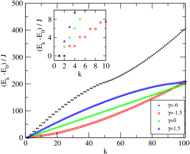
Figure 1: (Color online) Energy spectra for $N=100$ atoms and several values of $\gamma=-6,-1.5,0,1.5$. Only the excitation energies are plotted. The inset focuses in the lower eigenstates.

II.1 Spectral properties of the Bose-Hubbard Hamiltonian

The eigenfunctions and eigenvalues of the BH Hamiltonian (1) have been studied intensively Mil97 ; cirac98 ; jame05 ; vardi ; ST08 ; ours10 . For our subsequent discussion we only need to point out a couple of their properties. Figure 1 displays eigenvalues of $H_{BH}$ for several choices of $\gamma$. Note that, except for the appearance of quasi-doublets, the energy levels increase smoothly. Also, the figure exhibits, for $\gamma=\pm 1.5$, the symmetry in the spectral properties between repulsive (r) and attractive (a) interactions, $E_{k}^{(\rm r)}-E_{0}^{(\rm r)}=E_{N}^{(\rm a)}-E_{N-k}^{(\rm a)}$. The latter can be seen by noting that the BH Hamiltonians for attractive and repulsive interactions are related by a rotation around $\hat{J}_{y}$ of angle $\pi$ and an overall sign. The eigenstates for the repulsive and attractive case are also easily related by the same rotation.

II.2 Pseudo-spin formalism and coherent states

The state of a BJJ can be described by a large spin subject to a Hamiltonian that has both a linear and a non-linear term. As is customary LE01 , we introduce the “pseudo-spin” operators

$${\hat{J}}_{x} = \frac{1}{2}(\hat{a}_{1}^{{\dagger}}\hat{a}_{2}+\hat{a}_{2}^{{\dagger}}\hat{a}_{1})$$

$${\hat{J}}_{y} = \frac{1}{2i}(\hat{a}_{1}^{{\dagger}}\hat{a}_{2}-\hat{a}_{2}^{{\dagger}}\hat{a}_{1})$$

$${\hat{J}}_{z} = \frac{1}{2}(\hat{a}_{1}^{{\dagger}}\hat{a}_{1}-\hat{a}_{2}^{{\dagger}}\hat{a}_{2})$$ (4)

which satisfy the angular momentum commutation relations and

$${\hat{J}}_{x}^{2}+{\hat{J}}_{y}^{2}+{\hat{J}}_{z}^{2}=(N^{2}+2N)/4$$

on the $N$-boson space. In terms of these pseudo-spin operators,

$$H_{BH} = -2J{\hat{J}}_{x}+U{\hat{J}}_{z}^{2}+U\big{(}\tfrac{N^{2}}{4}-\tfrac{N}{2}\big{)}\ .$$ (5)

For any unit vector ${\bf u}=(u_{x},u_{y},u_{z})$, let

$${\hat{J}}_{\bf u}=u_{x}{\hat{J}}_{x}+u_{y}{\hat{J}}_{y}+u_{z}{\hat{J}}_{z}\ .$$

The eigenvectors of the pseudo-spin operators ${\hat{J}}_{\bf u}$ are the “coherent states” wherein all $N$ particles occupy the same mode husiref . Specifically, if $(\theta,\phi)$ are the spherical coordinates of a unit vector ${\bf u}$, so that

$$u_{x} = \sin\theta\cos\phi$$

$$u_{y} = \sin\theta\sin\phi$$

$$u_{z} = \cos\theta\ ,$$

then the coherent state $|\Psi_{\theta,\phi}^{N}\rangle$ defined by

$$|\Psi_{\theta,\phi}^{N}\rangle={1\over\sqrt{N!}}\left(\cos\theta/2\ a^{{\dagger}}_{1}+e^{i\phi}\sin\theta/2\ a^{{\dagger}}_{2}\right)^{N}|\O\rangle$$ (6)

is an eigenvector of ${\hat{J}}_{\bf u}$ with eigenvalue $N/2$.

Any pure state of $N$-bosons in a two-mode BJJ can be written as superposition of coherent states, for example by using the completeness relation husiref

$$\frac{1}{4\pi}\int_{0}^{\pi}\sin\theta d\theta\int_{0}^{2\pi}d\phi\ |\Psi_{\theta,\phi}^{N}\rangle\!\langle\Psi_{\theta,\phi}^{N}|\ =\frac{1}{N+1}$$ (7)

(note that $\sin\theta d\theta d\phi$ is the surface area element on the unit sphere). Though the coherent states form a complete set of $N$-particle states, they do not constitute an orthonormal basis; two coherent states are not orthogonal unless they correspond to antipodal points on the sphere.

We will also use the notation $(\hat{x},\hat{y},\hat{z})=\frac{2}{N}(\hat{J}_{x},\hat{J}_{y},\hat{J}_{z})$ for normalized pseudo-spin operators. The observable $\hat{z}$ is the population imbalance operator between the modes $\hat{a}_{1}^{{\dagger}}|\O\rangle$ and $\hat{a}_{2}^{{\dagger}}|\O\rangle$, normalized to have values between $-1$ and $+1$. The angular momentum commutation relations imply that

$$[\hat{x},\hat{y}]=\tfrac{2}{N}i\hat{z},\ \hbox{etc.,}\quad{\rm and}\;\hat{x}^{2}+\hat{y}^{2}+\hat{z}^{2}=1+\tfrac{2}{N}\ ,$$ (8)

which indicates that the average spin projections behave like classical observables in the limit $N\rightarrow\infty$.

II.3 Husimi distributions

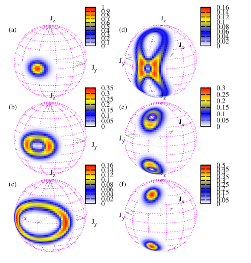
Figure 2: (Color online) Husimi distributions of some eigenvectors of the BH for $\gamma=1.5$. In panels (a), (b), (c), (d), (e), and (f), we plot the distributions corresponding to the states with index $k=0,2,10,90,98$, and 101, where $k=0$ is the ground state. $N=100$ particles.

When a state of a system of $N$ two-mode bosons is represented by a density matrix ${\hat{\rho}}$, the Husimi distribution, or Q representation, of that state is the function

$$P(\theta,\phi)=\langle\Psi_{\theta,\phi}^{N}|{\hat{\rho}}|\Psi_{\theta,\phi}^{N}\rangle$$ (9)

defined on the unit sphere lee84 ; mahmud05 .

The Husimi distribution of a pure state $|\Phi\rangle$ is just $\big{|}\langle\Psi_{\theta,\phi}^{N}|\Phi\rangle\big{|}^{2}$. For example, the Husimi distribution of the coherent state $|\Psi_{0,0}^{N}\rangle$ is $\big{|}\langle\Psi_{\theta,\phi}^{N}|\Psi_{0,0}^{N}\rangle\big{|}^{2}=\big{(}\cos^{2}(\theta/2)\big{)}^{N}$. The Husimi distribution of a coherent state $|\Psi_{\theta,\phi}^{N}\rangle$ is spread over the whole Bloch sphere, but as $N\rightarrow\infty$ the distribution becomes more and more concentrated about the point $(\theta,\phi)$.

Husimi distributions can help one visualize eigenstates of a Hamiltonian and see their connection to the classical orbits. Fig. 2 portrays the Husimi distribution of some eigenvectors of $H_{BH}$ for a characteristic repulsive interaction: $\gamma=1.5$. The ground state Husimi distribution in panel (a) is similar to that of the coherent state corresponding to the point $(\pi/2,0)$ on the Bloch sphere, but is somewhat flattened, reflecting the number-squeezing due to the repulsive interaction, as studied, e.g. in Ref. oursober . As the energy $E_{i}$ increases, the first Husimi distributions, graphed in panels (b) and (c), have the shape of elliptical rings of increasing size. Panels (e) and (f) show that the highest energy states have their Husimi distributions concentrated around the other classical stationary points of the Hamiltonian raghavan99 . Panel (d) shows the Husimi distribution before the transition to the highest energy states.

In this article, we are concerned with thermal equilibrium ensembles for $H_{BH}$, whose density matrices are the canonical ones. Thus, the Husimi distribution for the canonical ensemble of $N$ bosons at temperature $T$ is

$$P_{N,T}(\theta,\phi)\ =\ {\cal Z}^{-1}\ \sum_{i=0}^{N}e^{-E_{i}/k_{B}T}\big{|}\langle\Psi_{\theta,\phi}^{N}|\Phi_{i}\rangle\big{|}^{2}$$ (10)

where $|\Phi_{i}\rangle$ is the $i^{th}$ eigenstate of $H_{BH}$, with energy $E_{i}$, and

$${\cal Z}=\sum_{i=0}^{N}e^{-E_{i}/k_{B}T}$$

is the partition function. Note that the functions $\big{|}\langle\Psi_{\theta,\phi}^{N}|\Phi_{i}\rangle\big{|}^{2}$ appearing in (10) are the Husimi distributions of the eigenstates.

III Temperature effects

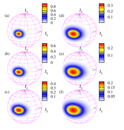
Figure 3: (Color online) Husimi distributions for $\gamma=1.5$ (repulsive interactions). From (a) to (f) the temperatures are $k_{B}T/(NJ)=0,0.25,0.5,0.75,1.,1.25$ and 1.5. $N=100$.

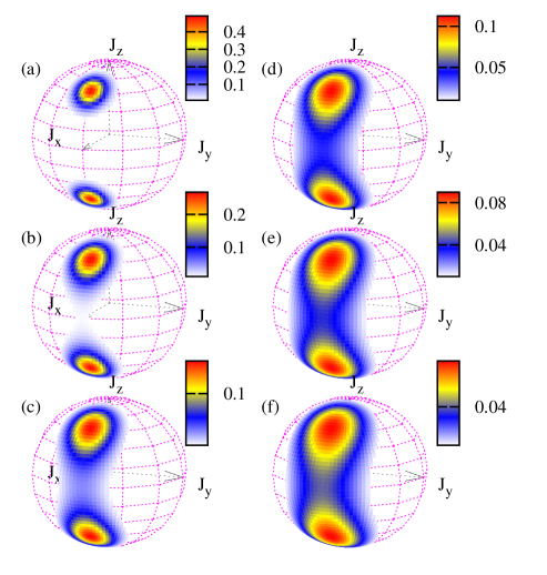
Figure 4: (Color online) Husimi distributions for $\gamma=-1.5$ (attractive interactions). From top to bottom and left to right the temperatures are $k_{B}T/(NJ)=0,0.25,0.5,0.75,1.,1.25$ and 1.5. $N=100$.

In this section we focus on the high temperature equilibrium behavior of BJJs in the Rabi-Josephson boundary regime GS09 where $|\gamma|\sim 1$. This regime can now be addressed experimentally in internal BJJs, where Feshbach resonances can be used to tune the interaction strength, and where the number of atoms is also relatively small (in the hundreds) zib10 . In the experiments reported in zibphd , for example, the number of atoms was around 300 and it was possible to control the value of $\gamma$ about $\gamma=-1$. We focus on the same regime of small $\gamma$ and relatively small $N$, but we consider relatively high temperatures $k_{B}T\sim NJ$. These temperatures are much higher than those relevant to the recent experiments just mentioned, where $k_{B}T\sim J$. Nevertheless, our exploration of the higher temperature behavior of the two-mode model should provide guidance for future experiments that may be performed in this regime.

To take a first look at the effect of higher temperatures in BJJs, we display the Husimi distributions of some of the canonical thermal equilibrium ensembles.

Figures 3 and 4 illustrate the change of the Husimi distributions of the canonical equilibrium ensembles as $T$ increases moderately. When $\gamma=+1.5$ one sees that the roughly elliptical shape remains, but covers a greater area on the Bloch sphere. The Husimi distributions for attractive interactions, shown in Fig. 4 for $\gamma=-1.5$, resemble the shapes of the Husimi distributions of the higher energy eigenstates for repulsive interactions, shown in panels (d)-(f) of Fig. 2. The reason for this is that the Husimi distribution of a thermal equilibrium distribution is a mixture of the Husimi distributions of the lower energy eigenstates (cf., formula (10)), and the Husimi distributions of low energy eigenstates for attractive interactions are identical to those of the corresponding high energy eigenstates for repulsive interactions, due to the spectral properties of the two-site Bose-Hubbard Hamiltonian mentioned in Sec. II.1.

We turn now to look at the behavior of the observables ${\hat{x}}$, ${\hat{y}}$, and ${\hat{z}}$. The average values $\langle{\hat{x}}\rangle$ and $\langle{\hat{z}}^{2}\rangle$ are of especial interest GO07 . They are used for quantifying spin-squeezing sore01 ; esteve08 ; gross12 and for noise thermometry ober06 ; noise_thermometer06 ; GS09 in BJJs.

The average $\alpha\equiv\langle\hat{x}\rangle$, called the coherence factor PS01 ; GO07 , is proportional to the mean fringe visibility in interference experiments. The coherence factor $\alpha$ is plotted in panels (b) and (d) of Figs. 5 and 6, respectively. We will consider the lower temperature ($k_{B}T\sim J$) behavior of the $\alpha$ in Sec. IV below.

The averages $\langle\hat{y}\rangle$ and $\langle\hat{z}\rangle$ are both equal to $0$ in the absence of any bias affecting ${\hat{J}}_{y}$ and ${\hat{J}}_{z}$. For this reason, $\langle\hat{y}^{2}\rangle$ and $\langle\hat{z}^{2}\rangle$ quantify the fluctuations of the observables ${\hat{y}}$ and ${\hat{z}}$ about their averages, and we shall accordingly use the notation $\Delta{\hat{y}}^{2}$ and $\Delta{\hat{z}}^{2}$ instead of $\langle\hat{y}^{2}\rangle$ and $\langle\hat{z}^{2}\rangle$. However, note that $\Delta{\hat{x}}^{2}=\langle{\hat{x}}^{2}\rangle-\langle{\hat{x}}\rangle^{2}$ is not the same as $\langle{\hat{x}}^{2}\rangle$ because $\langle{\hat{x}}\rangle\neq 0$.

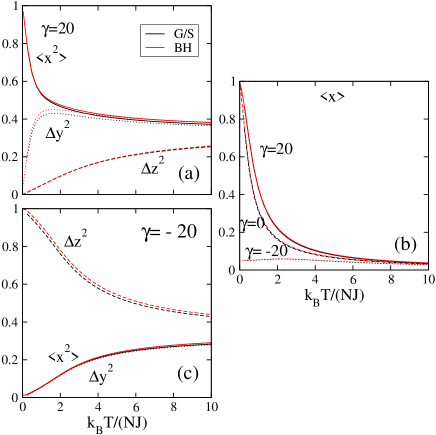
Figure 5: (Color online) Thermal averages for $\gamma=-20,0$ and $20$. Black lines show the prediction with the classical $N\to\infty$ approximation of Ref. GS09 while red ones are the BH results with $N=100$.

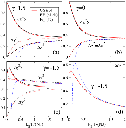
Figure 6: (Color online) Thermal averages for $\gamma=-1.5,0$ and $1.5$. Red lines are the prediction with the classical $N\to\infty$ approximation of Ref. GS09 while black ones are the BH results with $N=100$. The blue dot-dashed lines are the asymptotic GS predictions for large temperature given in (16) and (17).

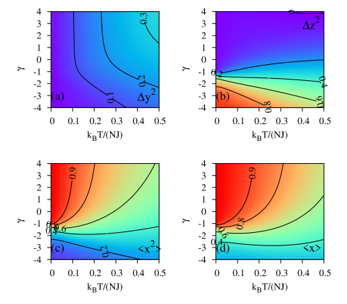
Figure 7: (Color online) Contour plots of $\Delta\hat{y}^{2}$, $\Delta\hat{z}^{2}$, $\langle\hat{x}^{2}\rangle$, and $\langle\hat{x}\rangle$ computed for Bose-Hubbard model with $N=100$, showing dependence on $T$ and $\gamma$.

To provide the overall picture, Fig. 7 displays the dependence of $\langle\hat{x}\rangle$, $\langle\hat{x}^{2}\rangle$, $\Delta\hat{y}^{2}$, and $\Delta\hat{z}^{2}$ on both $\gamma$ and $k_{B}T/(NJ)$. The figure is made for a fixed value of $N$, varying $\gamma$ and $T$. Note the abrupt change of behavior around $\gamma=-1$ and $T=0$. This reflects the bifurcation in the ground state properties there zib10 ; ours10 . For values of $\gamma<-1$ we have that $\langle\hat{x}^{2}\rangle$ and $\Delta\hat{y}^{2}$ remain small as $T$ increases, while $\Delta\hat{z}^{2}$ decreases from a value close to $1$ at $T=0$. On the other hand, for values of $\gamma>-1$, it is now $\langle\hat{x}^{2}\rangle$ that is close to 1 near $T=0$, while $\Delta\hat{y}^{2}$ and $\Delta\hat{z}^{2}$ are small.

Panels (a) and (c) of Figs. 5 and (a), (b) and (c) of 6 are plots of $\langle\hat{x}^{2}\rangle$, $\Delta\hat{y}^{2}$, and $\Delta\hat{z}^{2}$ for $\gamma=0,\pm 1.5$, and $\pm 20$. Note how quickly $\Delta{\hat{z}}^{2}$ drops with increasing $T$ when $\gamma=-1.5$ (panel (c) of Fig. 6). At zero temperature, $\Delta\hat{z}^{2}>0$ because the ground state is cat-like, but with a small increase in temperature $\Delta{\hat{z}}^{2}$ quickly drops 20% (with a concomitant increase in $\langle x^{2}\rangle$ and $\Delta{\hat{y}}^{2}$ due to the relation (8)).

IV Comparison with classical theory

In this section, we review the classical, i.e., $N\rightarrow\infty$, limit for the regime $k_{B}T\sim NJ$ and $|\gamma|\sim 1$. We shall see that the predictions of the classical theory are remarkably accurate even when $N$ is rather small.

IV.1 The classical theory

Following GS09 , we define dimensionless ratios which measure the tunneling and interaction energies with respect to the thermal energy, $k_{B}T$:

$$\delta=\frac{NJ}{k_{B}T}\qquad\hbox{and}\qquad\varepsilon=\frac{N^{2}U}{2k_{B}T}\ .$$

Note that $\gamma=\epsilon/\delta$. We prove in the appendix that the normalized Husimi distributions of the canonical equilibrium ensembles converge to a function proportional to

$$Q_{\delta,\epsilon}(\theta,\phi) = \exp(\delta\sin\theta\cos\phi-\varepsilon\cos^{2}\theta/2)$$ (11)

$$= \exp(\delta x-\varepsilon z^{2}/2)$$

in the limit $N\rightarrow\infty$ with $\delta$ and $\epsilon$ remaining constant.

According to the theorem stated in GS09 , canonical thermal ensemble averages of certain observables also converge in this limit. Let $O(\hat{x},\hat{y},\hat{z})$ denote any polynomial in the operators $\hat{x}$, $\hat{y}$, and $\hat{z}$, and let $\langle O(\hat{x},\hat{y},\hat{z})\rangle_{N,T}$ denote the canonical average value of the corresponding observable. Then $\langle O(\hat{x},\hat{y},\hat{z})\rangle_{N,T}$ tends to

$$\frac{1}{\cal N}\int_{S}e^{\delta x-\varepsilon z^{2}/2}\;O(x,y,z)\ dS$$ (12)

as $N\rightarrow\infty$ while $\delta$ and $\epsilon$ remain constant, where $dS$ denotes surface area measure on the unit sphere $S\ =\ \{(x,y,z):\ x^{2}+y^{2}+z^{2}=1\}$ and

$${\cal N}\ =\ \int_{S}e^{\delta x-\varepsilon z^{2}/2}dS\ .$$ (13)

The preceding theorem is also proved in the appendix, in a somewhat more general form. For the present, assuming that canonical equilibrium ensembles behave like statistical mixtures of coherent states when $N$ is large, let us explain where the weight function $\exp(\delta x-\varepsilon z^{2}/2)$ comes from:

In terms of the operators ${\hat{x}},{\hat{y}}$ and ${\hat{z}}$, the Hamiltonian reads

$$H_{BH}\ =\ -NJ{\hat{x}}+\tfrac{U}{4}N^{2}{\hat{z}}^{2}+U\big{(}\tfrac{N^{2}}{4}-\tfrac{N}{2}\big{)}\ .$$

The preceding Hamiltonian operator is considered as acting only upon the $N$-particle subspace of the boson Fock space. Accordingly, we drop the constant term and introduce $N$ explicitly into the notation for the Hamiltonian, defining

$$H_{N}\ =\ -NJ{\hat{x}}+\tfrac{U}{4}N^{2}{\hat{z}}^{2}\,.$$

In thermal equilibrium at temperature $T$, the statistical weight of the coherent state centered at the point $(\theta,\phi)$ in the Bloch sphere should be proportional to $\exp\big{(}-\tfrac{1}{k_{B}T}\langle\Psi_{\theta,\phi}^{N}|H_{N}|\Psi_{\theta,\phi}^{N}\rangle\big{)}$ because $\langle\Psi_{\theta,\phi}^{N}|H_{N}|\Psi_{\theta,\phi}^{N}\rangle$ is the energy of the coherent state. This equals

$$\exp\big{(}{\langle\Psi_{\theta,\phi}^{N}|\delta{\hat{x}}-\varepsilon{\hat{z}}^{2}/2|\Psi_{\theta,\phi}^{N}\rangle}\big{)}$$ (14)

since $-\tfrac{1}{k_{B}T}H_{N}=\delta\ {\hat{x}}-\varepsilon\ {\hat{z}}^{2}/2$. In the classical limit, (14) becomes $\exp(\delta x-\varepsilon z^{2}/2)$.

Using (12) one can compute expectations and variances of observables of interest. For example, one can calculate the coherence factor as follows. Defining $a\equiv\sqrt{1-x^{2}}$, the integral in (13) is

$${\cal N}\ =\ 2\int_{-1}^{1}\ e^{\delta x}\int_{-a}^{a}\ \frac{e^{-\varepsilon(a^{2}-y^{2})/2}}{\sqrt{a^{2}-y^{2}}}\ dy\ dx\ ,$$

where the factor $2$ takes into account the equal contributions of points with $z>0$ and $z<0$. Next, change $y=a\cos\xi$ so that $y\in(-a,a)$ implies that $\xi\in(0,\pi)$. Then,

$${\cal N}\ =\ \int_{-1}^{1}\ I_{0}\left(\tfrac{\varepsilon}{4}(1-x^{2})\right)\ e^{\delta x+\varepsilon x^{2}/4}\ dx\ .$$

Using the same changes of variable to rewrite the integral $\int xe^{\delta x-\varepsilon z^{2}/2}$, one arrives at the formula for the coherence factor given in Ref. GS09 :

$$\alpha_{\delta,\epsilon}\ =\ \frac{\int_{-1}^{1}\ x\ I_{0}\left(\frac{\varepsilon}{4}(1-x^{2})\right)\ e^{\delta x+\varepsilon x^{2}/4}\ dx}{\int_{-1}^{1}\ I_{0}\left(\frac{\varepsilon}{4}(1-x^{2})\right)\ e^{\delta x+\varepsilon x^{2}/4}\ dx}\ .$$ (15)

This formula for the coherence factor generalizes the one obtained in Ref. PS01 for the Josephson regime $\gamma\gg 1$.

When $k_{B}T$ is large compared to the energy parameters $NJ$ and $N^{2}U$, the dimensionless parameters $\delta$ and $\epsilon$ are small, and expected values as in (12) can be approximated by polynomials in $\delta$ and $\epsilon$. For example, using the formulas

$$\langle{\hat{x}}\rangle_{\delta,\epsilon} = \frac{\partial}{\partial\delta}\langle\log Q_{\delta,\epsilon}\rangle$$

$$\langle{\hat{z}^{2}}\rangle_{\delta,\epsilon} = -2\frac{\partial}{\partial\epsilon}\langle\log Q_{\delta,\epsilon}\rangle$$

and expanding the exponential $\exp(\delta x-\varepsilon z^{2}/2)$ in powers of $\delta$ and $\epsilon$, calculation shows that

$$\langle\hat{x}\rangle_{\delta,\epsilon} = \tfrac{1}{3}\delta+\tfrac{1}{45}\delta\epsilon$$ (16)

$$\langle\hat{z}^{2}\rangle_{\delta,\epsilon} = \tfrac{1}{3}-\tfrac{2}{45}\epsilon+\tfrac{2}{945}\epsilon^{2}-\tfrac{1}{45}\delta^{2}\,,$$ (17)

up to terms of third order in $\delta$ and $\epsilon$.

IV.2 Comparison of BH data to classical predictions

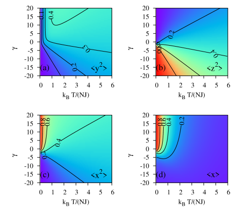
Figure 8: (Color online) Same description as Fig. 7 but computed with the GS approximation.

We now compare the results of our numerical solutions of the two-site Bose-Hubbard model for relatively small $N$ to the the predictions of the $N\rightarrow\infty$ limit discussed in the preceding paragraphs. In the following, “BH” refers to the Bose-Hubbard solutions for finite $N$ and “GS” or “classical” refers to the limit $N\rightarrow\infty$.

Figs. 5 and 6 show that the BH results are remarkably close to the classical predictions, both for attractive and repulsive interactions. Fig. 8 shows that the behavior around the transition at $\gamma=-1$ is well reproduced, as can be seen by comparing this figure with Fig. 7. This figure is similar to Fig. 7 but extends the range of parameters to higher $T$ and $|\gamma|$.

Fig. 6 compares the high temperature GS approximations (16) and (17) to the BH results. These simple approximations match the BH results quite well once $k_{B}T>NJ$.

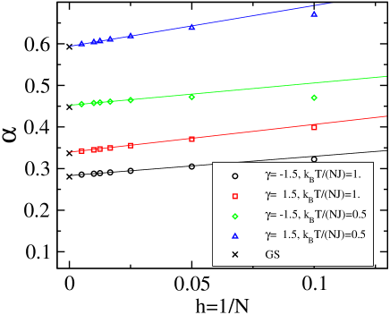
Figure 9: (Color online) Coherence factor $\alpha=\langle\hat{x}\rangle$ as a function of $1/N$ for two values of $k_{B}T/(NJ)=0.5$ and $=1$ and for two different values of $\gamma=\pm 1.5$. The thin lines are linear regression fits to the first three data points.

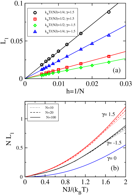
Figure 10: (Color online) (Top) Convergence of the BH Husimi distributions (18) to the classical limit (19) in terms of the averaged deviation (20). The solid lines are linear fits to the numerical results. (Bottom) Large temperature behavior of $NL_{1}$ for three different $N$ and $\gamma=0,\pm 1.5$. Note that we are plotting $NL_{1}$ against $\delta=NJ/k_{B}T$, not $J/k_{B}T$. The case $\gamma=0$ is computed with $N=100$.

Thus we see that the classical theory provides very good approximations even when $N\sim 100$. Deviations from the classical results at temperatures $k_{B}T\sim NJ$ are expected to be of order $1/N$. Fig. 9 shows how coherence factor converges to the GS prediction (15) as $1/N$ tends to $0$.

Finally, we look at how the Husimi distributions (10) converge to their classical limit (11). We normalize the Husimi distributions as is done in Ref. lee84 , making them probability density functions on the unit sphere. The normalized Husimi functions

$$\tilde{P}_{N,T}\ =\ \tfrac{N+1}{4\pi}P_{N,T}$$ (18)

with $P_{N,T}$ is as in (10), converge to

$$\tilde{Q}_{\delta,\epsilon}=\tfrac{1}{\cal N}Q_{\delta,\epsilon}$$ (19)

with $Q_{\delta,\epsilon}$ as in (11) and ${\cal N}$ as in (13). To see the rate of convergence we plot

$$L_{1}\ =\ \int_{S}\ \big{|}\tilde{P}_{N,T}-\tilde{Q}_{\delta,\epsilon}\big{|}\ dS$$ (20)

against $1/N$ in the top panel Fig. 10. The integrated absolute deviation $L_{1}$ appears proportional to $1/N$. The bottom panel of the same figure shows how the convergence rate depends on temperature. Plotting $NL_{1}$ against $NJ/k_{B}T$ indicates that $L_{1}\sim C(\gamma,T)/N$ with a small coefficient $C(\gamma,T)$ that decreases to $0$ as $T$ increases. In the non-interacting case $\gamma=0$, the Husimi distribution can be obtained exactly,

$$P_{N,T}^{\gamma=0}(\bar{\theta})={\xi-1\over\xi^{N+1}-1}\left({1+\xi+(\xi-1)\cos\bar{\theta}\over 2}\right)^{N}$$ (21)

with $\xi=e^{2\delta/N}$ and $\bar{\theta}$ the angle with respect to the $x$ axis. In this case, the $N\to\infty$ behavior of $NL_{1}$ can be shown to be quadratic in $\delta$, $NL_{1}=2/(9\sqrt{3})\delta^{2}+{\cal O}(\delta^{3})$.

IV.3 Lower temperatures

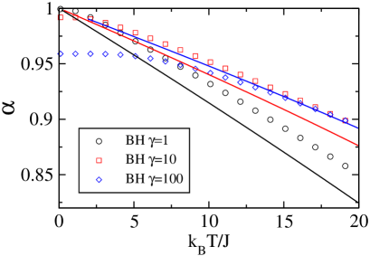
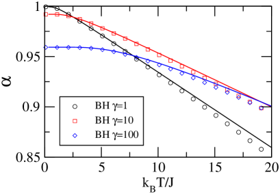
Figure 11: (Color online) Coherence factor of the system as a function of the temperature for several repulsive interactions, $\gamma=1,10$ and $100$, for $N=100$ atoms, focusing on the low temperature region where $k_{B}T\sim J$. The symbols represent the BH results, and the solid curves are obtained from eq. (15) in the top panel and eq. (22) in the bottom panel.

At temperatures $k_{B}T\sim J$, the number of eigenvectors contributing to the canonical equilibrium thermal ensemble is small, and the GS theory breaks down. As seen in the top panel of Fig. 11, the results of exact BH predict a sizable loss of coherence at low temperatures, whereas the GS formula (15) predicts full coherence as $T\rightarrow 0$.

Other approximations are available for this lower temperature regime ober06 ; malo13 . For repulsive atom-atom interactions, the $h=1/N$ expansion discussed in Ref. malo13 yields the following approximation of the coherence factor:

$$\alpha\ =\ {\cal A}-\frac{{\cal B}}{2}\left(\frac{N+1}{\tanh\beta F(N+1)}-\frac{1}{\tanh\beta F}-N\right)$$ (22)

with $\beta=1/k_{B}T$, $\;F=h\sqrt{\gamma+1-h}$, $\;{\cal B}=2h\frac{-\gamma/2-1+h}{\sqrt{\gamma+1-h}}$, and $\;{\cal A}=1+h+\tfrac{1}{2}{\cal B}$. The bottom panel of Fig. 11 shows that the incorporation of these $1/N$ effects produces very accurate results at $T\to 0$.

V Summary

We have studied effects of relatively high temperatures on bosonic Josephson junctions, focusing on both attractive and repulsive atom-atom interactions in the “Rabi-Josephson” boundary regime where $|\gamma|\sim 1$. Our study proceeded by solving the $N$-particle model Hamiltonian (a two-site Bose Hubbard model) for moderately small $N$ (around $100$) and comparing the results to the predictions of the “classical” limit attained as $N\rightarrow\infty$.

For temperatures much larger than the corresponding tunneling energy, the finite $N$ behavior (population imbalances and calculated Husimi distributions) is very close to the predictions of the classical limit, even for $N<100$. Differences between the “exact” finite-$N$ results and those of the classical limit appear to be proportional to $1/N$, with moderate correction coefficients.

The current study may contribute to an understanding of the way that higher temperatures wash out quantum effects expected at $T=0$. Our main conclusion is that, when the temperature in a bosonic Josephson junction is so high, quantum effects will only be seen if the number of particles is rather small.

Appendix A Proof of the convergence to the classical limit

In this appendix, we prove that the normalized Husimi distributions (18) converge to the classical limit (19), and then go on to prove the theorem of Ref. GS09 concerning canonical averages of $k$-particle correlations.

The Bose-Hubbard Hamiltonian on the $N$-boson space can be written

$$H_{N}\ =\ -J(\hat{a}_{1}^{{\dagger}}\hat{a}_{2}+\hat{a}_{2}^{{\dagger}}\hat{a}_{1})+\frac{U}{2}(\hat{a}_{1}^{{\dagger}}\hat{a}_{1}^{{\dagger}}\hat{a}_{1}\hat{a}_{1}+\hat{a}_{2}^{{\dagger}}\hat{a}_{2}^{{\dagger}}\hat{a}_{2}\hat{a}_{2})$$

$$= -\frac{J}{N}(\hat{a}_{1}^{{\dagger}}\hat{a}_{1}^{{\dagger}}\hat{a}_{1}\hat{a}_{2}+\hat{a}_{1}^{{\dagger}}\hat{a}_{2}^{{\dagger}}\hat{a}_{2}\hat{a}_{2}+\hat{a}_{2}^{{\dagger}}\hat{a}_{1}^{{\dagger}}\hat{a}_{1}\hat{a}_{1}+\hat{a}_{2}^{{\dagger}}\hat{a}_{2}^{{\dagger}}\hat{a}_{2}\hat{a}_{1})$$

$$+\ \frac{U}{2}(\hat{a}_{1}^{{\dagger}}\hat{a}_{1}^{{\dagger}}\hat{a}_{1}\hat{a}_{1}+\hat{a}_{2}^{{\dagger}}\hat{a}_{2}^{{\dagger}}\hat{a}_{2}\hat{a}_{2}).$$

In the preceding formula, operators like $\hat{a}_{1}^{{\dagger}}\hat{a}_{1}^{{\dagger}}\hat{a}_{1}\hat{a}_{2}$ are to be regarded as being restricted to the $N$-particle subspace, even though this is not indicated in the notation.

With the dimensionless parameters $\delta$ and $\epsilon$ defined in Sec. IV.1, we have $-\tfrac{1}{k_{B}T}H_{N}=\tfrac{1}{N^{2}}W_{N}$, where $W_{N}$ denotes the restriction of

$$W = \delta(\hat{a}_{1}^{{\dagger}}\hat{a}_{1}^{{\dagger}}\hat{a}_{1}\hat{a}_{2}+\hat{a}_{1}^{{\dagger}}\hat{a}_{2}^{{\dagger}}\hat{a}_{2}\hat{a}_{2}+\hat{a}_{2}^{{\dagger}}\hat{a}_{1}^{{\dagger}}\hat{a}_{1}\hat{a}_{1}+\hat{a}_{2}^{{\dagger}}\hat{a}_{2}^{{\dagger}}\hat{a}_{2}\hat{a}_{1})$$

$$-\epsilon(\hat{a}_{1}^{{\dagger}}\hat{a}_{1}^{{\dagger}}\hat{a}_{1}\hat{a}_{1}+\hat{a}_{2}^{{\dagger}}\hat{a}_{2}^{{\dagger}}\hat{a}_{2}\hat{a}_{2})$$

to the $N$-particle component of the boson Fock space. We are going to consider a limit where $N$ tends to infinity while $\delta$ and $\epsilon$ remain constant.

For each point on the Bloch sphere with spherical coordinates $(\theta,\phi)$, let

$$|\Psi_{\theta,\phi}\rangle\ =\ \big{(}\cos\tfrac{\theta}{2}\ a^{{\dagger}}_{1}+e^{i\phi}\sin\tfrac{\theta}{2}\ a^{{\dagger}}_{2}\big{)}|\O\rangle$$

denote the corresponding mode, and recall that $|\Psi_{\theta,\phi}^{N}\rangle$ denotes the coherent state of $N$ bosons in that mode (cf., formula (6)). Then, for any modes $|\chi_{1}\rangle,\ldots,|\chi_{n}\rangle$ and $|\chi^{\prime}_{1}\rangle,\ldots,|\chi^{\prime}_{n}\rangle$,

$$\big{\langle}\Psi_{\theta,\phi}^{N}\big{|}a^{\dagger}_{\chi_{1}}\cdots a^{\dagger}_{\chi_{n}}a_{\chi^{\prime}_{1}}\cdots a_{\chi^{\prime}_{n}}\Psi_{\theta,\phi}^{N}\big{\rangle}$$ (23)

$$= \ N^{(n)}\prod_{i=1}^{n}\langle\chi^{\prime}_{i}|\Psi_{\theta,\phi}\rangle\!\langle\Psi_{\theta,\phi}|\chi_{i}\rangle\ ,$$

where $N^{(n)}=\prod\limits_{m=0}^{n-1}(N-m)$. In particular, (23) implies that

$$\big{\langle}\Psi_{\theta,\phi}^{N}\big{|}W_{N}\Psi_{\theta,\phi}^{N}\big{\rangle}\ =\ N(N-1)(\delta x-\tfrac{1}{2}\epsilon z^{2}-\tfrac{1}{2}\epsilon)$$

with

$$x = \sin\theta\cos\phi$$

$$z = \cos\theta\ .$$

Let $\Xi$ denote a product of creators and annihilators which, when normally ordered, becomes

$$:\!\Xi\!:\ =\ a^{\dagger}_{\chi_{1}}\cdots a^{\dagger}_{\chi_{n}}a_{\chi^{\prime}_{1}}\cdots a_{\chi^{\prime}_{n}}.$$

Using the canonical commutation relations, formula (23) implies that

$$\lim\limits_{N\rightarrow\infty}\frac{1}{N^{n}}\big{\langle}\Psi_{\theta,\phi}^{N}\big{|}\Xi\Psi_{\theta,\phi}^{N}\big{\rangle}$$ (24)

$$= \lim\limits_{N\rightarrow\infty}\frac{1}{N^{n}}\big{\langle}\Psi_{\theta,\phi}^{N}\big{|}:\!\Xi\!:\Psi_{\theta,\phi}^{N}\big{\rangle}$$

$$= \prod_{i=1}^{n}\langle\chi^{\prime}_{i}|\Psi_{\theta,\phi}^{N}\rangle\!\langle\Psi_{\theta,\phi}^{N}|\chi_{i}\rangle\ .$$

Thus

$$\lim\limits_{N\rightarrow\infty}\frac{1}{N^{2j}}\big{\langle}\Psi_{\theta,\phi}^{N}\big{|}W_{N}^{j}\ \Psi_{\theta,\phi}^{N}\big{\rangle}$$

$$= \lim\limits_{N\rightarrow\infty}\frac{1}{N^{2j}}\big{\langle}\Psi_{\theta,\phi}^{N}\big{|}:\!W_{N}^{j}\!:\Psi_{\theta,\phi}^{N}\big{\rangle}\ =\ \left(\delta x-\tfrac{1}{2}\epsilon z-\tfrac{1}{2}\epsilon\right)^{j}$$

and therefore

$$\lim_{N\rightarrow\infty}\big{\langle}\Psi_{\theta,\phi}^{N}|e^{-H_{N}/k_{B}T}\Psi_{\theta,\phi}^{N}\big{\rangle}$$ (25)

$$= \lim_{N\rightarrow\infty}\big{\langle}\Psi_{\theta,\phi}^{N}|\exp(\tfrac{1}{N^{2}}W_{N})\Psi_{\theta,\phi}^{N}\big{\rangle}$$

$$= \sum_{j=0}^{\infty}\frac{1}{j!}\lim_{N\rightarrow\infty}\frac{1}{N^{2j}}\langle\Psi_{\theta,\phi}^{N}|W_{N}^{j}\Psi_{\theta,\phi}^{N}\rangle$$

$$= \exp\left(\delta x-\tfrac{\epsilon}{2}z^{2}-\tfrac{\epsilon}{2}\right)\,.$$

The Husimi distribution $P_{N,T}(\theta,\phi)$ defined in (10) is proportional to $\big{\langle}\Psi_{\theta,\phi}^{N}|e^{-H_{N}/k_{B}T}\Psi_{\theta,\phi}^{N}\big{\rangle}$. Its normalized version $\tilde{P}_{N,T}$ defined in formula (18) integrates to $1$. It follows from (25) that $\tilde{P}_{N,T}$ converges to $\tilde{Q}_{\delta,\epsilon}$ of formula (19) in the limit considered.

We now proceed to derive the theorem of Gottlieb and Schumm concerning canonical averages of $k$-particle correlations. This is the result that is paraphrased near the beginning of Section IV.1, but we prove it here in a slightly more general form, equivalent Theorem 1 of GS09 for the case of $M=2$ modes. That is, we prove the following:

Theorem 1

Let

$$X\ =\ a^{\dagger}_{\chi_{1}}\cdots a^{\dagger}_{\chi_{k}}a_{\chi^{\prime}_{1}}\cdots a_{\chi^{\prime}_{k}}$$

be a simple $k$-body operator. Then, in the limit where $N$ tends to infinity while $\delta$ and $\epsilon$ remain constant,

$$\lim_{N\rightarrow\infty}\frac{1}{N^{k}}\big{\langle}X\big{\rangle}_{N,T}$$

$$= \frac{1}{{\cal N}}\int_{S}dS\ \prod_{i=1}^{k}\langle\chi^{\prime}_{i}|\Psi_{\theta,\phi}\rangle\!\langle\Psi_{\theta,\phi}|\chi_{i}\rangle\ e^{\delta x-\tfrac{\epsilon}{2}z^{2}}\ ,$$

where ${\cal N}$ is the normalizing constant (13).

Proof:   As in formula (24), we have

$$\lim\limits_{N\rightarrow\infty}\frac{1}{N^{2j+k}}\big{\langle}\Psi_{\theta,\phi}^{N}\big{|}W_{N}^{j}X\ \Psi_{\theta,\phi}^{N}\big{\rangle}$$

$$= \lim\limits_{N\rightarrow\infty}\frac{1}{N^{2j+k}}\big{\langle}\Psi_{\theta,\phi}^{N}\big{|}:\!W_{N}^{j}X\!:\Psi_{\theta,\phi}^{N}\big{\rangle}$$

$$= \prod_{i=1}^{k}\langle\chi^{\prime}_{i}|\Psi_{\theta,\phi}^{N}\rangle\!\langle\Psi_{\theta,\phi}^{N}|\chi_{i}\rangle\left(\delta x-\tfrac{1}{2}\epsilon z^{2}-\tfrac{1}{2}\epsilon\right)^{j}.$$

Using the preceding formula and the completeness relation (7), i.e., the fact that

$$\frac{N+1}{4\pi}\int_{S}dS\big{|}\Psi_{\theta,\phi}^{N}\big{\rangle}\!\big{\langle}\Psi_{\theta,\phi}^{N}\big{|}$$

is the identity operator on the $N$-boson Hilbert space, we get

$$\lim_{N\rightarrow\infty}\frac{1}{N^{2j+k+1}}\hbox{Tr}(W_{N}^{j}X)$$

$$= \frac{1}{4\pi}\lim_{N\rightarrow\infty}\frac{N+1}{N^{2j+k+1}}\hbox{Tr}\left[W_{N}^{j}X\int_{S}dS\big{|}\Psi_{\theta,\phi}^{N}\big{\rangle}\!\big{\langle}\Psi_{\theta,\phi}^{N}\big{|}\right]$$

$$= \frac{1}{4\pi}\lim_{N\rightarrow\infty}\frac{1}{N^{2j+k}}\int_{S}dS\big{\langle}\Psi_{\theta,\phi}^{N}\big{|}W_{N}^{j}X\ \Psi_{\theta,\phi}^{N}\big{\rangle}$$

$$= \frac{1}{4\pi}\int_{S}dS\prod_{i=1}^{k}\langle\chi^{\prime}_{i}|\Psi_{\theta,\phi}^{N}\rangle\!\langle\Psi_{\theta,\phi}^{N}|\chi_{i}\rangle\left(\delta x-\tfrac{1}{2}\epsilon\ z^{2}-\tfrac{1}{2}\epsilon\right)^{j}$$

and therefore

$$\lim\limits_{N\rightarrow\infty}\frac{1}{N^{k+1}}\hbox{Tr}\big{[}e^{-H_{N}/k_{B}T}X\big{]}$$

$$= \lim_{N\rightarrow\infty}\frac{1}{N^{k+1}}\hbox{Tr}\Big{[}\exp(\tfrac{1}{N^{2}}W_{N})X\Big{]}$$

$$= \sum_{j=0}^{\infty}\frac{1}{j!}\lim_{N\rightarrow\infty}\frac{1}{N^{2j+k+1}}\hbox{Tr}(W_{N}^{j}X)$$

$$= \frac{e^{-\tfrac{\epsilon}{2}}}{4\pi}\int_{S}dS\ \prod_{i=1}^{k}\langle\chi^{\prime}_{i}|\Psi_{\theta,\phi}\rangle\!\langle\Psi_{\theta,\phi}|\chi_{i}\rangle\ e^{\delta x-\tfrac{\epsilon}{2}z^{2}}.$$

In particular,

$$\lim\limits_{N\rightarrow\infty}\frac{1}{N}\hbox{Tr}\big{[}e^{-H_{N}/k_{B}T}\big{]}\ =\ \frac{e^{-\tfrac{\epsilon}{2}}}{4\pi}\int_{S}dS\ e^{\delta x-\tfrac{\epsilon}{2}z^{2}}.$$

The two preceding limits imply that

$$\lim_{N\rightarrow\infty}\frac{1}{N^{k}}\big{\langle}a^{\dagger}_{\chi_{1}}\cdots a^{\dagger}_{\chi_{k}}a_{\chi^{\prime}_{1}}\cdots a_{\chi^{\prime}_{k}}\big{\rangle}_{N,T}$$

$$= \lim_{N\rightarrow\infty}\frac{1}{N^{k}}\frac{\hbox{Tr}\big{[}e^{-H_{N}/k_{B}T}X\big{]}}{\hbox{Tr}\big{[}e^{-H_{N}/k_{B}T}\big{]}}$$

$$= \frac{\lim\limits_{N\rightarrow\infty}\tfrac{1}{N^{k+1}}\hbox{Tr}\big{[}e^{-H_{N}/k_{B}T}X\big{]}}{\lim\limits_{N\rightarrow\infty}\tfrac{1}{N}\hbox{Tr}\big{[}e^{-H_{N}/k_{B}T}\big{]}}$$

$$= \frac{1}{{\cal N}}\int_{S}dS\ \prod_{i=1}^{k}\langle\chi^{\prime}_{i}|\Psi_{\theta,\phi}\rangle\!\langle\Psi_{\theta,\phi}|\chi_{i}\rangle e^{\delta x-\tfrac{\epsilon}{2}z^{2}}.$$

References

- (1) G.J. Milburn, J. Corney, E. M. Wright, and D. F. Walls, Phys. Rev. A 55, 4318 (1997).
- (2) A. Smerzi, S. Fantoni, S. Giovanazzi, and S. R. Shenoy, Phys. Rev. Lett. 79, 4950 (1997).
- (3) J. I. Cirac, M. Lewenstein, K. Molmer, and P. Zoller, Phys. Rev. A 57, 1208 (1998).
- (4) J. Javanainen M. Y. Ivanov Phys. Rev. A 60, 2351 (1999).
- (5) S. Raghavan, A. Smerzi, S. Fantoni, and S. R. Shenoy Phys. Rev. A 59, 620 (1999).
- (6) A. J. Leggett, Rev. Mod. Phys. 73, 307 (2001).
- (7) M. Jääskeläinen, and P. Meystre, Phys. Rev. A 71, 043603 (2005); Phys. Rev. A 73, 013602 (2006).
- (8) E. J. Mueller, T-L. Ho, M. Ueda, and G. Baym, Phys. Rev. A 74, 033612 (2006).
- (9) B. Juliá-Díaz, D. Dagnino, M. Lewenstein, J. Martorell, and A. Polls, Phys. Rev. A 81, 023615 (2010).
- (10) C. Ottaviani, V. Ahufinger, R. Corbalán, J. Mompart, Phys. Rev. A 81, 043621 (2010).
- (11) M. P. Strzys, E. M. Graefe and H. J. Korsch, New J. Phys. 10, 013024 (2008).
- (12) C. Khripkov, D. Cohen, A. Vardi, Phys. Rev. E 87, 012910 (2013).
- (13) M. Albiez, R. Gati, J. Fölling, S. Hunsmann, M. Cristiani, and M.K. Oberthaler, Phys. Rev. Lett. 95, 010402 (2005).
- (14) T. Zibold, E. Nicklas, C. Gross, and M. K. Oberthaler, Phys. Rev. Lett. 105, 204101 (2010).
- (15) C. Gross, J. Phys. B: At. Mol. Opt. Phys. 45, 103001 (2012).
- (16) H.J. Lipkin, N. Meshkov, and A.J. Glick, Nucl. Phys. 62, 188 (1965).
- (17) J. Esteve, C. Gross, A. Weller, S. Giovanazzi, and M. K. Oberthaler, Nature 455, 1216, (2008).
- (18) C. Gross, T. Zibold, E. Nicklas, J. Estève, and M. K. Oberthaler, Nature 464, 1165 (2010).
- (19) T. Zibold, PhD-Thesis: “Classical Bifurcation and Entanglement Generation in an Internal Bosonic Josephson Junction”, U. Heidelberg (2012).
- (20) B. Juliá-Díaz, J. Martorell, A. Polls, Phys. Rev. A 81, 063625 (2010).
- (21) M. Kitagawa, and M. Ueda, Phys. Rev. A 47, 5138 (1993).
- (22) J. R. Anglin, and, A. Vardi, Phys. Rev. A 64, 013605 (2001); A. Vardi, and J. R. Anglin, Phys. Rev. Lett. 86, 568 (2001).
- (23) L. Pitaevskii and S. Stringari, Phys. Rev. Lett. 87, 180402 (2001).
- (24) R. Gati and M.K. Oberthaler, J. Phys. B: At. Mol. Opt. Phys. 40, R61 (2007).
- (25) A.D. Gottlieb and T. Schumm, Phys. Rev. A 79, 063601 (2009)
- (26) R. Gati, B. Hemmerling, J. Fölling, M. Albiez, and M. K. Oberthaler Phys. Rev. Lett. 96, 130404 (2006).
- (27) B. Juliá-Díaz, J. Martorell, and A. Polls, Spontaneous symmetry breaking, self-trapping and Josephson oscillations, Progress in optical science and photonics, ed. B. Malomed, Springer (2013).
- (28) F. T. Arecchi, E. Courtens, R. Gilmore, and H. Thomas. Phys. Rev. A 6, 2211 (1972).
- (29) C.T. Lee, Phys. Rev. A 30 3308 - 3310
- (30) K. W. Mahmud, H. Perry, and W. P. Reinhardt, Phys. Rev. A 71, 023615 (2005).
- (31) B. Juliá-Díaz, T. Zibold, M. K. Oberthaler, M. Mele-Messeguer, J. Martorell, A. Polls, Phys. Rev. A 86, 023615 (2012).
- (32) A. S. Sørensen, L. M. Duan, J. I. Cirac, and P. Zoller, Nature 409, 63 (2001).
- (33) R. Gati, J. Esteve, Hemmerling, T. B. Ottenstein, J. Appmeier, A. Weller and. M K Oberthaler, New J. Phys. 8, 189 (2006).
- (34) V. S. Shchesnovich, and M. Trippenbach, Phys. Rev. A 78, 023611, (2008).