A new method of identifying self-similarity in isotropic turbulence

Abstract

In order to analyse results for structure functions, $S_{n}(r)$, we propose plotting the ratio $|S_{n}(r)/S_{3}(r)|$ against the separation $r$. This method differs from the extended self-similarity (ESS) technique, which plots $S_{n}(r)$ against $S_{3}(r)$, where $S_{3}(r)\sim r$. Using this method in conjunction with pseudospectral evaluation of structure functions, for the particular case of $S_{2}(r)$ we obtain the new result that the exponent $\zeta_{2}$ decreases as the Taylor-Reynolds number increases, with $\zeta_{2}\to 0.67\pm 0.02$ as $R_{\lambda}\to\infty$. This supports the idea of finite-viscosity corrections to the K41 prediction for $S_{2}$, and is the opposite of the result obtained by ESS.

In this Letter we revisit an old, but unresolved, issue in turbulence: the controversy that continues to surround the Kolmogorov theory (or K41) Kolmogorov (1941a, b). This controversy began with the publication in 1962 of Kolmogorov’s ‘refinement of previous hypotheses’, which gave a role to the intermittency of the dissipation rate Kolmogorov (1962). From this beginning, the search for ‘intermittency corrections’ has grown into a veritable industry over the years: for a general discussion, see the book Frisch (1995) and the review Boffetta et al. (2008). The term ‘intermittency corrections’ is rather tendentious, as no relationship has ever been demonstrated between intermittency, which is a property of a single realization, and the ensemble-averaged energy fluxes which underlie K41, and it is now increasingly replaced by ‘anomalous exponents’. It has also been observed by Kraichnan and others Kraichnan (1974); Saffman (1977); Sreenivasan (1999); Qian (2000), that the title of K62 is misleading. It in fact represents a profoundly different view of the underlying physics of turbulence, as compared to K41. For this reason alone it is important to resolve this controversy.

While this search has been a dominant theme in turbulence for many decades, at the same time there has been a small but significant number of theoretical papers exploring the effect of finite Reynolds numbers on the Kolmogorov exponents Effinger and Grossmann (1987); Barenblatt and Chorin (1998); Qian (2000); Gamard and George (1999); Lundgren (2002). All of these papers have something to say; but the last one is perhaps the most compelling, as it appears to offer a rigorous proof of the validity of K41 in the limit of infinite Reynolds number.

The controversy surrounding K41 basically amounts to: ‘intermittency corrections’ versus ‘finite Reynolds number effects’. The former are expected to increase with increasing Reynolds number, the latter to decrease. In time, direct numerical simulation (DNS) should establish the nature of high-Reynolds-number asymptotics, and so decide between the two. In the meantime, one would like to find some way of extracting the ‘signature’ of this information from current simulations.

As is well known, one way of doing this is by ESS. Our purpose here is to propose an alternative to ESS, in which we rely on a long-established technique in experimental physics, where the effective experimental error can be reduced by plotting the ratio of two dependent variables: see Chapter 3 in Bevington and Robinson (2003). Of course this does not work in all cases, but only where the quantities are positively correlated. We have verified that this is the case here and we will discuss these secondary aspects in a more extensive paper which we intend to submit as a regular article in due course. For the present, therefore, our proposal is that one should plot the ratio $|S_{n}(r)/S_{3}(r)|$ against the separation $r$. However, here we do this only for the case $n=2$, since K41 Kolmogorov (1941a, b) involves only $S_{2}$ and $S_{3}$, which are connected through energy conservation.

The study of turbulence structure functions (e.g. see van Atta and Chen (1970); Anselmet et al. (1984)) was transformed in the mid-1990s by the introduction of ESS by Benzi and co-workers Benzi et al. (1993, 1995). Their method of plotting results for $S_{n}(r)$ against $S_{3}(r)$, rather than against the separation $r$, showed extended regions of apparent scaling behaviour even at low-to-moderate values of the Reynolds number, and was widely taken up by others e.g. Fukayama et al. (2000); Stolovitzky et al. (1993); Meneveau (1996); Grossmann et al. (1997); Sain et al. (1998). A key feature of this work was the implication that corrections to the exponents of structure functions increase with increasing Reynolds number, which suggests that intermittency is the dominant effect.

The longitudinal structure functions are defined as

$$S_{n}(r)=\left\langle\delta u^{n}_{L}(r)\right\rangle\ ,$$ (1)

where the (longitudinal) velocity increment is given by

$$\delta u_{L}(r)=\Big{[}\boldsymbol{\mathbf{u}}(\boldsymbol{\mathbf{x}}+\boldsymbol{\mathbf{r}},t)-\boldsymbol{\mathbf{u}}(\boldsymbol{\mathbf{x}},t)\Big{]}\cdot\boldsymbol{\mathbf{\hat{r}}}\ .$$ (2)

Integration of the Kármán-Howarth equation (KHE) leads, in the limit of infinite Reynolds number, to the Kolmogorov ‘4/5’ law, $S_{3}(r)=-(4/5)\varepsilon r$. If the $S_{n}$, for $n\geq 4$, exhibit a range of power-law behaviour, then; in general, and solely on dimensional grounds, the structure functions of order $n$ are expected to take the form

$$S_{n}(r)=C_{n}(\varepsilon r)^{n/3}\ .$$ (3)

Measurement of the structure functions has repeatedly found a deviation from the above dimensional prediction for the exponents. If the structure functions are taken to scale with exponents $\zeta_{n}$, thus:

$$S_{n}(r)\sim r^{\zeta_{n}}\ ,$$ (4)

then it has been found Anselmet et al. (1984); Benzi et al. (1995) that the difference $\Delta_{n}=\lvert n/3-\zeta_{n}\rvert$ is non-zero and increases with order $n$. Exponents $\zeta_{n}$ which differ from $n/3$ are often referred to as anomalous exponents Benzi et al. (1995).

In order to study the behaviour of the exponents $\zeta_{n}$, it is usual to make a log-log plot of $S_{n}$ against $r$, and measure the local slope:

$$\zeta_{n}(r)=\frac{d\log{S_{n}(r)}}{d\log{r}}\ .$$ (5)

Following Fukayama et al Fukayama et al. (2000), the presence of a plateau when any $\zeta_{n}(r)$ is plotted against $r$ indicates a constant exponent, and hence a scaling region. Yet, it is not until comparatively high Reynolds numbers are attained that such a plateau is found. Instead, as seen in Fig. 1 (symbols), even for the relatively large value of Reynolds number, $R_{\lambda}=177$, a scaling region cannot be identified. (We note that Grossmann et al Grossmann et al. (1997) have argued that a minimum value of $R_{\lambda}\sim 500$ is needed for satisfactory direct measurement of local scaling exponents.)

Figure 1: Comparison of the local-slope exponents $\zeta_{n}(r)$ (symbols) for $n=2,4,6$ with the ESS exponents $\Sigma_{n}(r)$ (lines). Both sets of exponents were calculated from the real-space velocity field and are presented here for $R_{\lambda}=177$. The separation, $r$, has been scaled on the dissipation scale, $\eta=(\nu_{0}^{3}/\varepsilon)^{1/4}$.

The introduction of ESS relied on the fact that $S_{3}$ scales with $\zeta_{3}=1$ in the inertial range. Benzi et al Benzi et al. (1993) argued that

$$S_{n}(r)\sim[S_{3}(r)]^{\zeta^{*}_{n}}\ ,\quad\textrm{with}\quad\zeta^{*}_{n}=\zeta_{n}/\zeta_{3}\ .$$ (6)

$\zeta^{*}_{n}$ should then be equivalent to $\zeta_{n}$ in the scaling region.

A practical difficulty led to a further step. The statistical convergence of odd-order structure functions is significantly slower than that for even-orders, due to the delicate balance of positive and negative values involved in the former Fukayama et al. (2000). To overcome this, generalized structure functions have been introduced Benzi et al. (1993) (see also Stolovitzky et al. (1993); Fukayama et al. (2000)),

$$G_{n}(r)=\left\langle\lvert\delta u_{L}(r)\rvert^{n}\right\rangle\sim r^{\zeta^{\prime}_{n}},$$ (7)

with scaling exponents $\zeta^{\prime}_{n}$. The fact that $S_{3}\sim r$ in the inertial range does not rigorously imply that $G_{3}\sim r$ in the same range. But, by plotting $G_{3}(r)$ against $\lvert S_{3}(r)\rvert$, Benzi et al Benzi et al. (1995) showed that, for $R_{\lambda}=225$ – 800, the third-order exponents satisfied $\zeta^{\prime}_{3}\simeq 1.006\zeta_{3}$. Hence, it is now generally assumed that $\zeta^{\prime}_{n}$ and $\zeta_{n}$ are equal (although, Fig. 2 in Belin, Tabeling and Willaime Belin et al. (1996) implies some discrepancy at the largest length scales, and the authors note that the various exponents need not be the same). Thus, by extension, $G_{3}$ with $\zeta^{\prime}_{3}=1$, leads to

$$G_{n}(r)\sim[G_{3}(r)]^{\Sigma_{n}},\quad\textrm{with}\quad\Sigma_{n}=\zeta^{\prime}_{n}/\zeta^{\prime}_{3}\ .$$ (8)

Benzi et al Benzi et al. (1993) found that plotting their results on this basis gave a larger scaling region. This extended well into the dissipative lengthscales and allowed exponents to be more easily extracted from the data. Also, Grossmann et al Grossmann et al. (1997) state that the use of generalized structure functions is essential to take full advantage of ESS.

There is however an alternative to the use of generalized structure functions. This is the pseudospectral method. In using this for some of our work, we followed the example of Qian Qian (1997, 1999) and Tchoufag et al Tchoufag et al. (2012), who obtained $S_{2}$ and $S_{3}$ from the energy and energy transfer spectra, respectively, by means of exact quadratures.

The organization of our own work in this Letter is now as follows. We illustrate ESS, using results from our own simulations. We also show that our results for ESS agree closely with those of other investigations Benzi et al. (1995); Fukayama et al. (2000). We obtained these particular results in the usual way by direct convolution sums, using a statistical ensemble, and the generalized structure functions. We next investigated our new method, for six Reynolds numbers spanning the range $101.3\leq R_{\lambda}\leq 335.2$. To do this we employed the pseudospectral method Qian (1997, 1999); Tchoufag et al. (2012).

We begin by illustrating the use of ESS in Fig. 1, where we have plotted the ESS exponents $\Sigma_{n}$, for $n=2$, 4 and 6, as lines. They may be compared to the corresponding values of $\zeta_{n}$, plotted as symbols. The difference between the two sets of results is obvious. The plots of $\zeta_{n}$ show no sign of scaling behaviour. In complete contrast, the plots of $\Sigma_{n}$ against $r$ consist almost entirely of plateaux, even extending well into the dissipation range, where there would be no expectation of power-law behaviour.

It should also be noted, that we divided each exponent by the relevant $n/3$ in order to conveniently put the two sets of results on the same graph. Bearing this in mind, we see that, as $r\to 0$, the exponents $\zeta_{n}(r)\to n$ while $\Sigma_{n}(r)\to n/3$. This K41-type behaviour of the $\Sigma_{n}$ (which is not expected for values of $r$ in the dissipation range) arises because of the behaviour of the $\zeta_{n}$ at small $r$, in itself a consequence of the regularity of the velocity field. As was pointed out by Barenblatt et al Barenblatt et al. (1999), who described it as an artefact, this had been recognized from the outset by Benzi et al Benzi et al. (1993).

We used a standard pseudospectral DNS for a periodic box of side $L_{\textrm{box}}=2\pi$, with full dealiasing performed by truncation according to the 2/3 rule. For each Reynolds number studied, we used the same initial spectrum ($k^{4}$ for the low-$k$ modes) and input rate $\varepsilon_{W}$. Stationarity was maintained using negative damping, with $\boldsymbol{\mathbf{f}}(\boldsymbol{\mathbf{k}},t)=(\varepsilon_{W}/2E_{f})\boldsymbol{\mathbf{u}}(\boldsymbol{\mathbf{k}},t)$ for modes with $\lvert\boldsymbol{\mathbf{k}}\rvert<k_{f}=2.5$, where $E_{f}$ is the total energy contained in the forced band. The only initial condition changed was the value assigned to the (kinematic) viscosity, $\nu_{0}$. An ensemble of $M$ realizations was generated by sampling the velocity every half a large-eddy turnover time, $L/U$. The simulations are summarized in Table 1, and our ESS results are plotted in Fig. 1 for $R_{\lambda}=177$, and later in Fig. 3.

$R_{\lambda}$	$\nu_{0}$	$N$	$\varepsilon$	$U$	$L/L_{\text{box}}$	$k_{\text{max}}\eta$	$M$
42.5	0.01	128	0.094	0.581	0.23	2.34	101
64.2	0.005	128	0.099	0.607	0.21	1.37	101
101.3	0.002	256	0.099	0.607	0.19	1.41	101
113.3	0.0018	256	0.100	0.626	0.20	1.31
176.9	0.00072	512	0.102	0.626	0.19	1.31	15
203.7	0.0005	512	0.099	0.608	0.18	1.01
276.2	0.0003	1024	0.100	0.626	0.18	1.38
335.2	0.0002	1024	0.102	0.626	0.18	1.01

Table 1: A summary of the numerical simulations which have been performed. The ensemble size, $M$, is given for those runs for which the ESS method has been performed.

In order to examine our new proposal, we used the six runs listed in Table 1 with Reynolds numbers in the range $101.3\leq R_{\lambda}\leq 335.2$, in conjunction with the pseudospectral method. The second- and third-order structure functions were found from the energy and transfer spectra, respectively, $E(k)$ and $T(k)$, using Fourier transforms: See Monin and Yaglom Monin and Yaglom (1975), equations (12.75) and (12.141^′′′). This spectral approach has the consequence that we are now evaluating the conventional structure functions, as defined by equations (1) and (2), rather than the generalized structure functions, $G_{n}(r)$, as commonly used (including by us) for ESS.

Pseudospectral calculations of the structure functions were carried out for $R_{\lambda}=101$ and 177 (and found to be comparable to the calculations in real space); and for the further values of the Reynolds numbers of 113, 204, 276 and 335, which were used in Figures 2 and 3.

We now arrive at the main point of this Letter, which is to introduce a new local-scaling exponent $\Gamma_{n}$, which can be used instead to determine the $\zeta_{n}$. We work with $S_{n}(r)$ and consider the quantity $\lvert S_{n}(r)/S_{3}(r)\rvert$. In this procedure, the exponent $\Gamma_{n}$ is defined by

$$\left\lvert\frac{S_{n}(r)}{S_{3}(r)}\right\rvert\sim r^{\Gamma_{n}}\ ,\qquad\text{where}\qquad\Gamma_{n}=\zeta_{n}-\zeta_{3}\ .$$ (9)

This idea is tested, for the case $n=2$, in Fig. 2. The dimensionless quantity $U\lvert S_{2}(r)/S_{3}(r)\rvert$, where $U$ is the rms velocity, is plotted against $r/\eta$, for three values of $R_{\lambda}$. Note that, since K41 predicts $\Gamma_{2}=-1/3$, we have plotted a compensated form, in which we multiply the ratio by $(r/\eta)^{1/3}$, such that K41 scaling would correspond to a plateau. From the figure, we can see a trend towards K41 scaling as the Reynolds number is increased.

Figure 2: Compensated ratio $(r/\eta)^{1/3}U\lvert S_{2}(r)/S_{3}(r)\rvert$ plotted against $r$, scaled on the dissipation scale, $\eta$. K41 scaling would correspond to a plateau. Arrows indicate $\lambda/\eta$, while the vertical dotted lines show the region used to fit each exponent.

Note that this figure also illustrates the ranges used to find values for our new exponent $\Gamma_{2}$, for the following cases. $\Gamma_{2}$ was fitted to the ranges $\lambda<r<c\lambda$, with $c=2.0,2.5$ and 3.0 for $R_{\lambda}=101,177$ and 335, respectively.

It should be emphasised that with both methods it is necessary to take $\zeta_{3}=1$ in the inertial range, in order to obtain the inertial-range value of either $\Sigma_{2}=\zeta_{2}$ (by ESS) or $\Gamma_{2}=\zeta_{2}-1$ (our new method). For this reason, we plot $\Gamma_{2}+1$, rather than $\Gamma_{2}$ in Fig. 3. From a comparison of Figs. 1 and 2, an obvious difference between our proposed method and ESS is apparent as $r\to 0$. This is readily understood in terms of the regularity condition for the velocity field, which leads to $S_{n}(r)\sim r^{n}$ as $r\to 0$ Stolovitzky et al. (1993); Sirovich et al. (1994). This yields $\Gamma_{n}(r)+1\to n-2$, whereas ESS gives $\zeta^{*}_{n}(r)\to n/3$.

Figure 3 summarizes the comparison between our results for our new method of determining the second-order exponent and those based on ESS (our own and others Benzi et al. (1995); Fukayama et al. (2000)) or on direct measurement Gotoh et al. (2002), in terms of their overall dependence on the Taylor-Reynolds number. In order to establish the form of the dependence of the exponents on Reynolds number, we fitted curves to the data points using the nonlinear-least-squares Marquardt-Levenberg algorithm, with the error quoted being one standard error. First we fitted a curve $\Gamma_{2}+1=A+BR_{\lambda}^{p}$, to find the asymptotic value $A=0.67\pm 0.02$. Then we fitted the curve $\Sigma_{2}=C+DR_{\lambda}^{q}$, using our data and that of Fukayama et al Fukayama et al. (2000). Evidently the two fitted curves show very different trends, with results for $\Sigma_{2}$ increasing with increasing Reynolds number, whereas $\zeta_{2}=\Gamma_{2}+1$ decreases and approaches 2/3 as $R_{\lambda}$ increases.

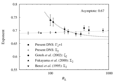
Figure 3: Dependence of our new exponent $\zeta_{2}=\Gamma_{2}+1$ on Reynolds number, compared to other measured exponents: Fukayama et al Fukayama et al. (2000), Gotoh et al Gotoh et al. (2002) and Benzi et al Benzi et al. (1995). The horizontal line indicates the K41 value of 2/3. The dashed line indicates the fit to $\Gamma_{2}+1$, while the dash-dot line shows a fit to $\Sigma_{2}$ using our results and those of Fukayama et al Fukayama et al. (2000).

As we have said, the point at issue is essentially ‘intermittency corrections versus finite Reynolds number effects’. The former has received much more attention; but, in recent years, there has been a growing interest in studying finite Reynolds number effects, experimentally and by DNS, for the case of $S_{3}$: see Tchoufag et al. (2012); Gotoh et al. (2002); Antonia and Burattini (2006) and references therein. (Although we note that in this case the emphasis is on the prefactor rather than the exponent.)

Our new result that $\zeta_{2}=\Gamma_{2}+1\to 2/3$ may be the first indication that anomalous values of $\zeta_{2}$ are due to finite Reynolds number effects. Previously it was suggested by Barenblatt et al that ESS could be interpreted in this way Barenblatt et al. (1999), but this was disputed by Benzi et al Benzi et al. (1999).

There is much remaining to be understood about these matters and we suggest that our new method of analysing data can help. It should, of course, be noted that our use of $S_{3}$ (as evaluated by pseudospectral methods) rather than $G_{3}$ (as used with ESS), may also be a factor in our new result. In an extended account of this work (now in preparation) we will give a full explanation of the motivation and the circumstances under which it can be expected to work. As a matter of interest, we conclude by noting that our analysis can also provide a motivation for ESS and may lead to an understanding of the relationship between the two methods. It is also the case that the pseudospectral method could be used for the general study of higher-order structure functions, but this awaits the derivation of the requisite Fourier transforms.

The authors would like to thank Matthew Salewski, who read a first draft and made many helpful suggestions. SY and AB were funded by the STFC.

References

- Kolmogorov (1941a) A. N. Kolmogorov, C. R. Acad. Sci. URSS 30, 301 (1941a).
- Kolmogorov (1941b) A. N. Kolmogorov, C. R. Acad. Sci. URSS 32, 16 (1941b).
- Kolmogorov (1962) A. N. Kolmogorov, J. Fluid Mech. 13, 82 (1962).
- Frisch (1995) U. Frisch, Turbulence: the legacy of A. N. Kolmogorov (Cambridge University Press, 1995).
- Boffetta et al. (2008) G. Boffetta, A. Mazzino, and A. Vulpiani, J. Phys. A: Math. Theor. 41, 363001 (2008).
- Kraichnan (1974) R. H. Kraichnan, J. Fluid Mech. 62, 305 (1974).
- Saffman (1977) P. G. Saffman, in Structure and Mechanisms of Turbulence II, edited by H. Fiedler (Springer-Verlag, 1977), vol. 76 of Lecture Notes in Physics, pp. 273–306.
- Sreenivasan (1999) K. R. Sreenivasan, Rev. Mod. Phys. 71, S383 (1999).
- Qian (2000) J. Qian, Physical Review Letters 84, 646 (2000).
- Effinger and Grossmann (1987) H. Effinger and S. Grossmann, Z. Phys. B 66, 289 (1987).
- Barenblatt and Chorin (1998) G. I. Barenblatt and A. J. Chorin, SIAM Rev. 40, 265 (1998).
- Gamard and George (1999) S. Gamard and W. K. George, Flow, turbulence and combustion 63, 443 (1999).
- Lundgren (2002) T. S. Lundgren, Phys. Fluids 14, 638 (2002).
- Bevington and Robinson (2003) P. R. Bevington and D. K. Robinson, Data Reduction and Error Analysis for the Physical Sciences (McGraw-Hill, 2003), 3rd ed.
- van Atta and Chen (1970) C. W. van Atta and W. Y. Chen, J. Fluid Mech. 44, 145 (1970).
- Anselmet et al. (1984) F. Anselmet, Y. Gagne, E. J. Hopfinger, and R. A. Antonia, J. Fluid Mech. 140, 63 (1984).
- Benzi et al. (1993) R. Benzi, S. Ciliberto, R. Tripiccione, C. Baudet, F. Massaioli, and S. Succi, Phys. Rev. E 48, R29 (1993).
- Benzi et al. (1995) R. Benzi, S. Ciliberto, C. Baudet, and G. R. Chavarria, Physica D: Nonlinear Phenomena 80, 385 (1995).
- Fukayama et al. (2000) D. Fukayama, T. Oyamada, T. Nakano, T. Gotoh, and K. Yamamoto, J. Phys. Soc. Japan 69, 701 (2000).
- Stolovitzky et al. (1993) G. Stolovitzky, K. R. Sreenivasan, and A. Juneja, Phys. Rev. E 48, R3217 (1993).
- Meneveau (1996) C. Meneveau, Phys. Rev. E 54, 3657 (1996).
- Grossmann et al. (1997) S. Grossmann, D. Lohse, and A. Reeh, Phys. Rev. E 56, 5473 (1997).
- Sain et al. (1998) A. Sain, Manu, and R. Pandit, Phys. Rev. Lett. 81, 4377 (1998).
- Belin et al. (1996) F. Belin, P. Tabeling, and H. Willaime, Physica D 93, 52 (1996).
- Qian (1997) J. Qian, Physical Review E 55, 337 (1997).
- Qian (1999) J. Qian, Physical Review E 60, 3409 (1999).
- Tchoufag et al. (2012) J. Tchoufag, P. Sagaut, and C. Cambon, Phys. Fluids 24, 015107 (2012).
- Barenblatt et al. (1999) G. I. Barenblatt, A. J. Chorin, and V. M. Prostokishin, Physica D 127, 105 (1999).
- Monin and Yaglom (1975) A. S. Monin and A. M. Yaglom, Statistical Fluid Mechanics (MIT Press, 1975).
- Sirovich et al. (1994) L. Sirovich, L. Smith, and V. Yakhot, Phys. Rev. Lett. 72, 344 (1994).
- Gotoh et al. (2002) T. Gotoh, D. Fukayama, and T. Nakano, Phys. Fluids 14, 1065 (2002).
- Antonia and Burattini (2006) R. A. Antonia and P. Burattini, J. Fluid Mech. 550, 175 (2006).
- Benzi et al. (1999) R. Benzi, S. Ciliberto, C. Baudet, and G. Ruiz-Chavarria, Physica D 127, 111 (1999).