Analysis of the Taylor dissipation surrogate in forced isotropic turbulence

Abstract

From the energy balance in wavenumber space expressed by the Lin equation, we derive a new form for the local Karman-Howarth equation for forced isotropic turbulence in real space. This equation is then cast into a dimensionless form, from which a combined analytical and numerical study leads us to deduce a new model for the scale-independent nondimensional dissipation rate $C_{\varepsilon}$, which takes the form $C_{\varepsilon}=C_{\varepsilon,\infty}+C_{L}/R_{L}$, where the asymptotic value $C_{\varepsilon,\infty}$ can be evaluated from the third-order structure function. This is found to fit the numerical data with $C_{\varepsilon,\infty}=0.47\pm 0.01$ and $C_{L}=18.5\pm 1.3$. By considering $C_{\varepsilon}-C_{\varepsilon,\infty}$ on logarithmic scales, we show that $R_{L}^{-1}$ is indeed the correct Reynolds number behaviour. The model is compared to previous attempts in the literature, with encouraging agreement. The effects of the scale-dependence of the inertial and viscous terms due to finite forcing are then considered and shown to compensate one another, such that the model equation is applicable for systems subject to finite forcing. In addition, we also show that, contrary to the case of freely decaying turbulence, the characteristic decline in $C_{\varepsilon}$ with increasing Reynolds number is due to the increase in the surrogate expression $U^{3}/L$; the dissipation rate being maintained constant as a consequence of the fixed rate of forcing. A long-time non-turbulent stable state is found to exist for low Reynolds number numerical simulations which use negative damping as a means of energy injection.

I Introduction

In recent years there has been much interest in the fundamentals of turbulent dissipation. This interest has centred on the approximate expression for the dissipation rate $\varepsilon$ which was given by Taylor in 1935 Taylor (1935) as

$$\varepsilon=C_{\varepsilon}U^{3}/L,$$ (1)

where $U$ is the root-mean-square velocity and $L$ is the integral scale. Many workers in the field refer to equation (1) as the Taylor dissipation surrogate. However, others rearrange it to define the coefficient $C_{\varepsilon}$ as the nondimensional dissipation rate, thus:

$$C_{\varepsilon}=\frac{\varepsilon}{U^{3}/L}.$$ (2)

In 1953 Batchelor Batchelor (1971) presented evidence to suggest that the coefficient $C_{\varepsilon}$ tended to a constant value with increasing Reynolds number. In 1984 Sreenivasan Sreenivasan (1984) showed that in grid turbulence $C_{\varepsilon}$ became constant for Taylor-Reynolds numbers greater than about $50$. Later still, in 1998, he presented a survey of investigations of both forced and decaying turbulence Sreenivasan (1998), using direct numerical simulation (DNS), which established the now characteristic curve of $C_{\varepsilon}$ plotted against the Taylor-Reynolds number $R_{\lambda}$.

In his 1968 lecture notes Saffman (1968), Saffman made two comments about the expression that we have given here as equation (1). These were: “This result is fundamental to an understanding of turbulence and yet still lacks theoretical support” and “the possibility that $A$ (i.e. our $C_{\varepsilon}$) depends weakly on the Reynolds number can by no means be completely discounted”. More than forty years on, the question implicit in his second comment has been comprehensively answered by the survey papers of Sreenivasan Sreenivasan (1984, 1998), along with a great deal of subsequent work by others, some of which we have cited here. However, while some theoretical work has indicated an inverse proportionality between $C_{\varepsilon}$ and Reynolds number, this has been limited to low (i.e. non-turbulent) Reynolds numbers Sreenivasan (1984) or based on a mean-field approximation Lohse (1994) or restricted to providing an upper-bound Doering and Foias (2002). Hence his first comment is still valid today; and this lack of theoretical support remains one of the main impediments to the development of turbulence phenomenology and hence turbulence theory.

As we have seen before, an approach based on the dimensionless dissipation $C_{\varepsilon}$, the ratio of the dissipation to the surrogate expression $U^{3}/L$, can be a helpful way of looking at things McComb et al. (2010). In the present paper, we examine the behaviour of $C_{\varepsilon}$ with increasing Reynolds number by means of a simple model based on the Karman-Howarth equation and supported by direct numerical simulation (DNS). We find that this description captures the observed dependence of $C_{\varepsilon}$, thus providing a direct theoretical route from the Navier-Stokes equation to dissipation rate scaling. We begin with a description of our DNS, before presenting a theoretical analysis followed by numerical results.

II The numerical simulations

We used a pseudospectral DNS, with full dealiasing performed by truncation of the velocity field according to the two-thirds rule. Time advancement for the viscous term was performed exactly using an integrating factor, while the non-linear term used Heun’s method (second-order predictor-corrector). Each run was started from a Gaussian-distributed random field with a specified energy spectrum (which behaves as $k^{4}$ for the low-$k$ modes), and was allowed to a reach steady-state before measurements were made. A deterministic forcing scheme was employed, with the force $\boldsymbol{\mathbf{f}}$ given by

$$\boldsymbol{\mathbf{f}}(\boldsymbol{\mathbf{k}},t) =(\varepsilon_{W}/2E_{f})\boldsymbol{\mathbf{u}}(\boldsymbol{\mathbf{k}},t)\quad\text{for}\quad 0<\lvert\boldsymbol{\mathbf{k}}\rvert<k_{f};$$

$$=0\quad\textrm{otherwise},$$ (3)

where $\boldsymbol{\mathbf{u}}(\boldsymbol{\mathbf{k}},t)$ is the instantaneous velocity field (in wavenumber space). The highest forced wavenumber, $k_{f}$, was chosen to be $k_{f}=2.5$. As $E_{f}$ was the total energy contained in the forcing band, this ensured that the energy injection rate was $\varepsilon_{W}=\textrm{constant}$. It is worth noting that any method of energy injection employed in the numerical simulation of isotropic turbulence is not experimentally realisable. The present method of negative damping has also been used in other investigations Jiménez et al. (1993); Yamazaki et al. (2002); Kaneda et al. (2003); Kaneda and Ishihara (2006), albeit not necessarily such that $\varepsilon_{W}$ is maintained constant (although note the theoretical analysis of this type of forcing by Doering and Petrov Doering and Petrov (2005)), and we stress that at no point do we rely on the fact that the force is correlated with the velocity.

For each Reynolds number studied, we used the same initial spectrum and input rate $\varepsilon_{W}$. The only initial condition changed was the value assigned to the (kinematic) viscosity. Once the initial transient had passed the velocity field was sampled every half a large-eddy turnover time, $\tau=L/U$. The ensemble populated with these sampled realisations was used, in conjunction with the usual shell averaging, to calculate statistics. Simulations were run using lattices of size $64^{3},\ 128^{3},\ 256^{3},\ 512^{3}$ and $1024^{3}$, with corresponding Reynolds numbers ranging from $R_{\lambda}=8.40$ up to $335.2$. The smallest resolved wavenumber was $k_{\text{min}}=2\pi/L_{\text{box}}=1$ in all simulations, while the maximum wavenumber always satisfied $k_{\text{max}}\eta>1.0$, where $\eta$ is the Kolmogorov dissipation lengthscale. The integral scale, $L$, was found to lie between $0.34L_{\text{box}}$ and $0.18L_{\text{box}}$. Details of the individual runs are summarised in table 1.

$R_{\lambda}$	$\nu_{0}$	$N$	$\varepsilon$	$\sigma$	$U$	$L/L_{\text{box}}$	$k_{\text{max}}\eta$
8.40	0.09	64	0.085	0.011	0.435	0.34	6.09
9.91	0.07	64	0.081	0.014	0.440	0.32	5.10
13.9	0.05	64	0.086	0.014	0.485	0.31	3.91
24.7	0.02	64	0.092	0.011	0.523	0.24	1.93
41.8	0.01	512	0.097	0.010	0.581	0.22	9.57
42.5	0.01	128	0.094	0.015	0.581	0.23	2.34
44.0	0.009	128	0.096	0.009	0.587	0.22	2.15
48.0	0.008	128	0.096	0.013	0.586	0.22	1.96
49.6	0.007	128	0.098	0.011	0.579	0.20	1.77
60.8	0.005	512	0.098	0.009	0.589	0.20	5.68
64.2	0.005	128	0.099	0.011	0.607	0.21	1.37
89.4	0.0025	512	0.101	0.006	0.605	0.19	3.35
101.3	0.002	256	0.099	0.009	0.607	0.19	1.41
113.3	0.0018	256	0.100	0.008	0.626	0.20	1.31
153.4	0.001	512	0.098	0.011	0.626	0.20	1.70
176.9	0.00072	512	0.102	0.009	0.626	0.19	1.31
203.7	0.0005	512	0.099	0.008	0.608	0.18	1.01
276.2	0.0003	1024	0.100	0.009	0.626	0.18	1.38
335.2	0.0002	1024	0.102	0.008	0.626	0.18	1.01

Table 1: A summary of the main parameters for our numerical simulations. The values quoted for the dissipation rate $\varepsilon$ and its standard deviation $\sigma$, the total energy $E$ and the velocity-derivative skewness $S$, are ensemble- and shell-averaged mean values.

In addition, we note that all data fitting has been performed using an implementation of the nonlinear-least-squares Marquardt-Levenberg algorithm, with the error quoted being one standard error.

Figure 1: Variation of the dimensionless dissipation coefficient with Taylor-Reynolds number. Other investigations of forced turbulence are presented for comparison.

Our simulations have been well validated by means of extensive and detailed comparison with the results of other investigations. These include the Taylor-Green vortex Taylor and Green (1937); Brachet et al. (1983); measurements of the isotropy, Kolmogorov constant and velocity-derivative skewness; advection of a passive scalar; and a direct comparison with the freely-available pseudospectral code hit3d . These will be presented in another paper, but it can be seen from Fig. 1 that our results reproduce the characteristic behaviour for the plot of $C_{\varepsilon}$ against $R_{\lambda}$, and agree closely with other representative results in the literature Wang et al. (1996); Cao et al. (1999); Gotoh et al. (2002); Kaneda et al. (2003); Donzis et al. (2005). We note that the data presented for comparison was obtained using negative-damping (with variable $\varepsilon_{W}$) Kaneda et al. (2003), stochastic noise Gotoh et al. (2002); Donzis et al. (2005), or maintaining a $k^{-5/3}$ energy spectrum within the forced shells Wang et al. (1996); Cao et al. (1999). These methods for energy injection have been discussed in Bos et al. (2007).

III A Dimensionless Karman-Howarth equation for forced turbulence

The use of stirring forces with the energy equation in spectral space (i.e. with the Lin equation) is well established,

$$\frac{\partial E(k)}{\partial t}=T(k)-2\nu_{0}k^{2}+W(k)\ ,$$ (4)

where $\nu_{0}$ is the kinematic viscosity, $E(k)$ and $T(k)$ are the energy and transfer spectra, respectively, and $W(k)=4\pi k^{2}\langle\boldsymbol{\mathbf{u}}(-\boldsymbol{\mathbf{k}})\cdot\boldsymbol{\mathbf{f}}(\boldsymbol{\mathbf{k}})\rangle$ is the work spectrum of the stirring force, $\boldsymbol{\mathbf{f}}(\boldsymbol{\mathbf{k}})$. (See, for example, McComb (1990).) But this is not the case with the Karman-Howarth equation (KHE), which is its real-space equivalent. Accordingly, we obtain the equivalent KHE by Fourier transformation of the Lin equation (with forcing) as

$$-\frac{3}{2}\frac{\partial U^{2}}{\partial t}+\frac{3}{4}\frac{\partial S_{2}(r)}{\partial t} =-\frac{1}{4r^{4}}\frac{\partial}{\partial r}\Big{(}r^{4}S_{3}(r)\Big{)}$$ (5)

$$\qquad+\frac{3\nu_{0}}{2r^{4}}\frac{\partial}{\partial r}\left(r^{4}\frac{\partial S_{2}(r)}{\partial r}\right)-I(r)\ ,$$

where the longitudinal structure functions are defined as

$$S_{n}(r)=\left\langle\big{(}[\boldsymbol{\mathbf{u}}(\boldsymbol{\mathbf{x}}+\boldsymbol{\mathbf{r}})-\boldsymbol{\mathbf{u}}(\boldsymbol{\mathbf{x}})]\cdot\boldsymbol{\mathbf{\hat{r}}}\big{)}^{n}\right\rangle\ .$$ (6)

The input $I(r)$ is given in terms of $W(k)$, the work spectrum of the stirring forces, by

$$I(r) =3\int_{0}^{\infty}dk\ W(k)\ \left[\frac{\sin{kr}-kr\cos{kr}}{(kr)^{3}}\right]\ .$$ (7)

Here $I(r)$ is interpreted as the total energy injected into all scales $>r$. Note that we may make the connection between $W(k)$ and the injection rate for the numerical simulations by

$$I(0)=\int^{\infty}_{0}dk\,W(k)=\varepsilon_{W}\ ,$$ (8)

where the energy injection rate $\varepsilon_{W}$ is defined in (3).

If we were to apply (5) to freely-decaying turbulence, we would set the input term $I(r)$ equal to zero, to give:

$$-\frac{3}{2}\frac{\partial U^{2}}{\partial t}=-\frac{3}{4}\frac{\partial S_{2}}{\partial t}-\frac{1}{4r^{4}}\frac{\partial}{\partial r}\Big{(}r^{4}S_{3}\Big{)}+\frac{3\nu_{0}}{2r^{4}}\frac{\partial}{\partial r}\left(r^{4}\frac{\partial S_{2}}{\partial r}\right)\ .$$ (9)

Of course, for the case of free decay, we may also set $(3/2)\partial U^{2}/\partial t=-\varepsilon$, after which we obtain the form of the KHE which is familiar in the literature (e.g. see Monin and Yaglom (1975)). However, this can lead to problems if this substitution is retained for forced turbulence, for which it is not valid.

If, on the other hand, we are considering forced turbulence which has reached a stationary state, then we may set $\partial U^{2}/\partial t=\partial S_{2}/\partial t=0$, whereupon (5) reduces to the appropriate KHE for forced turbulence,

$$I(r)=-\frac{1}{4r^{4}}\frac{\partial}{\partial r}\Big{(}r^{4}S_{3}(r)\Big{)}+\frac{3\nu_{0}}{2r^{4}}\frac{\partial}{\partial r}\left(r^{4}\frac{\partial S_{2}(r)}{\partial r}\right)\ .$$ (10)

As an aside, we note that this form for the forced KHE has several important differences from other approaches which have appeared in the literature Sirovich et al. (1994); Gotoh et al. (2002). Previous approaches incorrectly retained the dissipation rate in the equation and essentially introduced an approximate ad hoc ‘correction’ in order to take account of the forcing. This is, for example, presented for the third-order structure function as

$$S_{3}(r)=-\frac{4\varepsilon r}{5}+Z(r)+6\nu_{0}\frac{\partial S_{2}}{\partial r}\ ,$$ (11)

where $Z(r)$ is the ad hoc correction Gotoh et al. (2002). In contrast, we note that the origin of $\varepsilon$ in the KHE was $\partial U^{2}/\partial t$, which is zero for a stationary system, and instead show how its role is now played by the energy input function, $I(r)$. Thus, in our approach, instead of equation (11), we have

$$S_{3}(r)=-\frac{4}{r^{4}}\int_{0}^{r}dy\ y^{4}I(y)+6\nu_{0}\frac{\partial S_{2}}{\partial r}\ ,$$ (12)

where $I(r)$ is calculated directly from the work spectrum, and is not approximated. Taking the limit $r\to 0$ in equation (7), for small scales we measure $I(r)=\varepsilon_{W}=\varepsilon$, and so recover the Kolmogorov form of the KHE equation Kolmogorov (1941).

Returning to our form of the forced KHE, equation (10), we now introduce the dimensionless structure functions $h_{n}(\rho)$ which are given by

$$S_{n}(r)=U^{n}h_{n}(\rho)\ ,$$ (13)

where $\rho=r/L$. Substitution into (10) leads to

$$-\frac{1}{4\rho^{4}}\frac{\partial}{\partial\rho}\Big{(}\rho^{4}h_{3}(\rho)\Big{)}\frac{U^{3}}{L}\equiv A_{3}(\rho|R_{L})\frac{U^{3}}{L}\ ;$$ (14)

$$\frac{3}{2\rho^{4}}\frac{\partial}{\partial\rho}\left(\rho^{4}\frac{\partial h_{2}(\rho)}{\partial\rho}\right)\frac{\nu_{0}U^{2}}{L^{2}}\equiv\frac{A_{2}(\rho|R_{L})}{R_{L}}\frac{U^{3}}{L}\ ,$$ (15)

with $R_{L}=UL/\nu_{0}$ the Reynolds number based on the integral scale. This introduces the coefficients $A_{3}$ and $A_{2}$, which are readily seen to be

$$A_{3}(\rho|R_{L}) =-\frac{1}{4\rho^{4}}\frac{\partial}{\partial\rho}\Big{(}\rho^{4}h_{3}(\rho)\Big{)}$$

$$A_{2}(\rho|R_{L}) =\frac{3}{2\rho^{4}}\frac{\partial}{\partial\rho}\left(\rho^{4}\frac{\partial h_{2}(\rho)}{\partial\rho}\right)\ .$$ (16)

Then, with some rearrangement, the forced KHE (10) takes the dimensionless form

$$I(\rho)\frac{L}{U^{3}}=A_{3}(\rho|R_{L})+\frac{A_{2}(\rho|R_{L})}{R_{L}}\ .$$ (17)

This simple scaling analysis has extracted the integral scale as the relevant lengthscale, and $R_{L}$ as the appropriate Reynolds number, for studying the behaviour of $C_{\varepsilon}$. This was noted by Batchelor Batchelor (1953), despite which it has become common practice to study $C_{\varepsilon}=C_{\varepsilon}(R_{\lambda})$, as demonstrated by Fig. 1.

The input term may be expressed as an amplitude and a dimensionless shape function,

$$I(\rho)=\varepsilon_{W}\phi(\rho)\ ,$$ (18)

where $\phi(\rho)$ contains all of the scale-dependent information and, as required by equation (8), satisfies $\phi(0)=1$.

III.1 The limit of $\delta(\boldsymbol{\mathbf{k}})$-forcing

Figure 2 illustrates the shape of $\phi(\rho)$ and shows the effect of varying the forcing band defined in equation (3), using data from our $R_{\lambda}=276$ run.

Figure 2: The dimensionless input shape function $\phi(\rho)$, as defined by equation (18). The effect of varying the forcing band, $0<k<k_{f}$, is illustrated, showing the limit of $\delta(\boldsymbol{\mathbf{k}})$-forcing. Presented for $R_{\lambda}=276$ data.

As we reduce the width of the forcing band, we approach the limit of $\delta$-function forcing in wavenumber space, corresponding to $\phi(\rho)=1\ \forall\rho$. This cannot be studied using DNS, since the zero mode is not coupled to any other mode (and indeed is symmetry-breaking). But, for theoretical convenience, we consider the limit analytically (or, alternatively, restrict our attention to scales for which $\phi(\rho)\simeq 1$) before addressing the complication added by scale dependence.

Now let us consider the dimensionless KHE for the case of $\delta(\mathbf{k})$-forcing, where $I(\rho)=\varepsilon_{W}=\varepsilon$. Equation (17) becomes

$$\frac{\varepsilon_{W}L}{U^{3}}=A_{3}(\rho|R_{L})+\frac{A_{2}(\rho|R_{L})}{R_{L}}\ ,$$ (19)

from which, since $\varepsilon=\varepsilon_{W}$ and using equation (2), we have

$$C_{\varepsilon}=A_{3}(\rho|R_{L})+\frac{A_{2}(\rho|R_{L})}{R_{L}}\ .$$ (20)

From the well known phenomenology associated with Kolmogorov’s inertial-range theories Kolmogorov (1941), as the Reynolds number tends to infinity, we know that we must have $A_{2}/R_{L}\to 0$ and $A_{3}\to C_{\varepsilon,\infty}\equiv\mbox{constant}$. Hence, this equation suggests the possibility of a simple model of the form

$$C_{\varepsilon}=C_{\varepsilon,\infty}+\frac{C_{L}}{R_{L}}\ ,$$ (21)

where $C_{\varepsilon,\infty}$ and $C_{L}$ are constants.

Equation (20) can also be rewritten as

$$\varepsilon=A_{3}(\rho|R_{L})\frac{U^{3}}{L}+A_{2}(\rho|R_{L})\frac{\nu_{0}U^{2}}{L^{2}}\ .$$ (22)

The first term on the RHS is essentially the Taylor surrogate, while the second term is a viscous correction. It has been shown McComb et al. (2010) that, for the case of decaying turbulence, the surrogate $U^{3}/L$ behaves more like a lumped-parameter representation for the maximum inertial transfer, $\varepsilon_{T}$, than the dissipation rate. The same is shown later for forced turbulence in Fig. 3, since the input rate (hence $\varepsilon$) is kept constant. Thus, the forced KHE is expressing the equivalence of the rate at which energy is transferred and dissipated (or injected) as $\nu_{0}\to 0$. At finite viscosity, there is a contribution to the dissipation rate which has not passed through the cascade. In terms of our model equation,

$$\varepsilon=C_{\varepsilon,\infty}\frac{U^{3}}{L}+\nu_{0}C_{L}\frac{U^{2}}{L^{2}}\to\varepsilon_{T}\qquad\text{as}\qquad\nu_{0}\to 0\ ,$$ (23)

where, from equation (16), the asymptotic value is given by the expression

$$C_{\varepsilon,\infty}=\lim_{\nu_{0}\to 0}A_{3}(\rho|R_{L})=-\frac{L}{U^{3}}\lim_{\nu_{0}\to 0}\frac{1}{4r^{4}}\frac{\partial}{\partial r}\left(r^{4}S_{3}(r)\right)\ .$$ (24)

III.2 Modelling the scale dependence of coefficients with an ad hoc profile function

We now address the fact that the coefficients $A_{3}(\rho)$ and $A_{2}(\rho)$ are not constants. They are separately scale-dependent; and, in general, may also have a parametric dependence on the Reynolds number.

To begin, we use $\varepsilon_{W}=\varepsilon$ to rewrite equation (18) as $I(\rho)L/U^{3}=C_{\varepsilon}\phi(\rho)$, such that equation (17) becomes

$$C_{\varepsilon}=\frac{A_{3}(\rho|R_{L})}{\phi(\rho)}+\frac{A_{2}(\rho|R_{L})}{R_{L}\phi(\rho)}\ .$$ (25)

However, the fact that the left hand side of (25) is constant with respect to the dimensionless scale $\rho=r/L$ means that the separate dependences on $\rho$ on the right hand side must cancel. In order to separate out the scale-dependent effects, we seek semi-empirical decompositions for $A_{3}(\rho)$ and $A_{2}(\rho)$ which satisfy the following conditions:

1. The $\rho$-dependence of the terms on the RHS of (25) must cancel, since the LHS is a constant;

2. As $\rho\to 0$, we have $A_{3}(\rho)/\phi(\rho)\to 0$ and so $A_{2}(\rho)/R_{L}\phi(\rho)\to C_{\varepsilon}(R_{L})$ (it is entirely viscous);

3. As $\rho\to\infty$, we have $A_{2}(\rho)\to 0$ and $A_{3}(\rho)/\phi(\rho)\to C_{\varepsilon}(R_{L})$ (it is entirely inertial);

4. As $R_{L}\to\infty$: $C_{\varepsilon}(R_{L})\to C_{\varepsilon,\infty}=\text{constant}$.

It is easily verified that these constraints are satisfied by the following expressions,

$$\frac{A_{3}(\rho|R_{L})}{\phi(\rho)} =C_{\varepsilon}\left[1-H(\rho)\right];\quad\text{and}$$ (26)

$$\frac{A_{2}(\rho|R_{L})}{R_{L}\phi(\rho)} =C_{\varepsilon}H(\rho)\ ,$$ (27)

where we have introduced an ad hoc profile function $H(\rho)$, which in general must satisfy the conditions:

$$\lim_{\rho\to 0}H(\rho)=1\quad\mbox{and}\quad\lim_{\rho\to\infty}H(\rho)=0.$$ (28)

The behaviour of the profile function at small and intermediate scales is also constrained by our knowledge of the structure functions. At small scales, the structure functions behave as $S_{n}\sim r^{n}$, which implies that $H(\rho)\simeq 1-a\rho^{2}$ for some $a$. For large enough Reynolds numbers, in the inertial range of scales $S_{2}\sim r^{\gamma}$ which leads to $H(\rho)\sim\rho^{\gamma-2}$, with $\gamma(R_{L})\to 2/3$ as $R_{L}$ is increased. Based on these additional constraints, we have chosen a suitable profile function to represent the scale dependence to be

$$H(\rho)=\left[1+\frac{a\rho^{2}}{1+b\rho^{\gamma}}\right]^{-1}\ ,$$ (29)

where $a$, $b$ and $\gamma$ are Reynolds number dependent and obtained by fitting to numerical results. We note that the actual values of these fit parameters do not affect our model (21) since the scale dependence cancels out.

IV Numerical results

Figure 3: Variation with Taylor-Reynolds number of the dissipation rate $\varepsilon$, maximum inertial transfer $\varepsilon_{T}$ and Taylor surrogate $U^{3}/L$. Values to the left of the dashed line should be treated with caution: see the discussion in Section IV regarding Fig. 4.

In Fig. 3 we show separately the behaviour of the dissipation rate $\varepsilon$, the maximum inertial flux $\varepsilon_{T}$ and the Taylor surrogate $U^{3}/L$, where each of these quantities was scaled on the constant injection rate $\varepsilon_{W}$. This is the basis of our first observation. We see that the decrease of $C_{\varepsilon}$, with increasing Reynolds number, is caused by the increasing value of the surrogate in the denominator, rather than by decay of the dissipation rate in the numerator, as this remains fixed at $\varepsilon=\varepsilon_{W}$. This is the exact opposite of the case for freely decaying turbulence, where the actual dissipation rate decreases with increasing Reynolds number, while the surrogate remains fairly constant McComb et al. (2010). The figure also shows how $U^{3}/L$ is a better lumped-parameter representation for $\varepsilon_{T}$ than $\varepsilon$ and that $\varepsilon/\varepsilon_{T}\to 1$ from above as the Reynolds number is increased, corresponding to the onset of an inertial range McComb (1990).

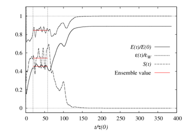
(a)

(b)

Figure 4: (a) Variation in time of the dissipation rate, total energy and skewness, $S$, for our lowest value of the Reynolds number, $R_{\lambda}=8.40$. The times usually associated with the steady state are indicated by vertical dotted lines, with the ensemble values highlighted. For $t>150\tau(0)$, we see a non-turbulent stable state. (b) Evolution of the energy spectrum from the ensemble averaged region through the transition to a stable, non-turbulent state. Error bars represent 3 standard deviations.

Note that all but the lowest two Reynolds number simulations conserved energy to within one standard deviation ($\sigma$) of the dissipation rate. However, runs with $R_{\lambda}<25$ (indicated by the vertical dashed line in Fig. 3) should be treated with caution. A significant deviation from $\varepsilon=\varepsilon_{W}$ in a stationary simulation is an indication that the simulation is yet to reach steady state. A simulation to determine the long-time properties of these low Reynolds number runs was performed, with interesting results. As shown in Fig. 4(a), after the time usually associated with the steady state (indicated by vertical dotted lines), the simulation developed into a stationary stable state. This non-turbulent state has zero skewness, and essentially involves only one excited wavenumber, $k=1$; see Fig. 4(b). The ensemble averaged energy spectrum has been calculated within the times indicated by vertical dotted lines in Fig. 4(a). Also plotted are the energy spectra at $t=90\tau(0),\ 150\tau(0)$ and $300\tau(0)$, corresponding to times within, towards the end of, and after the transition from pseudo-steady state to non-turbulent stable state, respectively. We see the development of a single-mode energy spectrum, with all the energy eventually being contained in the mode $k=1$.

This phenomenon has important consequences for the validity of all forced DNS results employing negative-damping, not just our own. It is currently unclear whether or not all Reynolds numbers will eventually develop into a stable, non-turbulent state, and one always measures a transient state masquerading as a steady state in which $\varepsilon$ fluctuates around a mean value which approaches $\varepsilon_{W}$ as Reynolds number is increased.

If instead this non-turbulent state is a low Reynolds number property, an alternative explanation for measuring $\varepsilon<\varepsilon_{W}$ involves the resolution of the large scales. It is becoming increasingly common to note that we do not only need to ensure that DNS is resolving the small, dissipative scales, but also the large, energy containing scales, such as $L$. It is possible that this apparent lack of conservation of energy is caused by $L/L_{\text{box}}$ too large.

Further investigation is clearly needed. Until such information is available, we follow the literature and continue to use our DNS data for $R_{\lambda}>25$. Despite simulations with lower Reynolds numbers being reported in the literature ($R_{\lambda}=8$ Donzis et al. (2005)) without energy conservation necessarily having been verified, our data corresponding to $R_{\lambda}<25$ will not be taken into account on the basis that, for whatever reason, the simulation did not conserve energy.

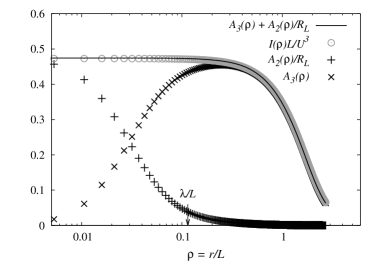
Figure 5: Dimensionless energy balance in the Karman-Howarth equation, as expressed by equation (17). $R_{\lambda}=276$. The Taylor microscale is labelled for comparison.

Figure 5 shows the balance of energy represented by the dimensionless equation given as (17). For small scales ($\rho<0.2$ for the case $R_{\lambda}=276$ shown) the input term satisfies $I(r)\simeq\varepsilon_{W}=\varepsilon$, as expected since such scales are not directly influenced by the forcing. We note that the second- and third-order structure functions may be obtained from the energy and transfer spectra, respectively, using

$$S_{2}(r) =4\int dk\ E(k)\ a(kr);$$

$$S_{3}(r) =12\int dk\ \frac{T(k)}{k^{2}}\frac{\partial a(kr)}{\partial r}\ ,$$ (30)

where the function $a(x)$ is:

$$a(x)=\frac{1}{3}-\frac{\sin{x}-x\cos{x}}{x^{3}},$$ (31)

with the derivatives of $a(kr)$ calculated analytically. This procedure was introduced by Qian Qian (1997, 1999) and more recently used by Tchoufag et al Tchoufag et al. (2012): the underlying transforms may be found in the book by Monin and Yaglom Monin and Yaglom (1975): equations (12.75) and (12.141^′′′). From these expressions, the non-linear and viscous terms, $A_{3}$ and $A_{2}$ given by equation (16), have been calculated using:

$$A_{3}(\rho) =-\frac{3L}{U^{3}}\int_{0}^{\infty}dk\ T(k)\left[\frac{\sin{kL\rho}-kL\rho\cos{kL\rho}}{(kL\rho)^{3}}\right]$$

$$A_{2}(\rho) =\frac{6\nu_{0}L}{U^{3}}\int_{0}^{\infty}dk\ k^{2}E(k)\left[\frac{\sin{kL\rho}-kL\rho\cos{kL\rho}}{(kL\rho)^{3}}\right].$$ (32)

In order to test our model for the dimensionless dissipation rate, we fitted an expression of the form (21), but with an arbitrary power-law dependence $R_{L}^{p}$, to data obtained with the present DNS, and it was found to agree very well, as shown in figure 6(a). The exponent was found to be $p=-1.00\pm 0.02$ and so supports the model equation, with the constants given by $C_{\varepsilon,\infty}=0.47\pm 0.01$ and $C_{L}=18.5\pm 1.3$.

A more graphic demonstration of this fact is given in Fig. 6(b). The standard procedure of using a log-log plot to identify power-law behaviour is unavailable in this case, due to the asymptotic constant. For this reason, we subtracted the estimated asymptotic value, and plotted $C_{\varepsilon}-C_{\varepsilon,\infty}$ against $R_{L}$ on logarithmic scales. This allowed us to identify power-law behaviour consistent with $R_{L}^{-1}$. We also tested the effect of varying our estimate of the value of the asymptote $C_{\varepsilon,\infty}$. It can be seen that the results were insensitive to this at the lower Reynolds numbers, where the $R_{L}^{-1}$ is being tested. At higher $R_{L}$, the viscous contribution represented by $C_{L}/R_{L}$ becomes negligible and instead we become strongly dependent on the actual value of $C_{\varepsilon,\infty}$.

(a)

(b)

Figure 6: (a) The expression given in equation (21) fitted to present DNS data. (b) Log-log plot of the present DNS results for $C_{\varepsilon}$ against Reynolds number, once the estimate of the asymptote is subtracted. The solid line represents a slope of $-1.00$. The effect of varying our estimate of the asymptote $C_{\varepsilon,\infty}$ is shown by the three symbols.

This model should be compared to other work in the literature. Sreenivasan Sreenivasan (1984) compared experimental decaying results to the expression for very low Reynolds numbers,

$$C_{\varepsilon}=\frac{15}{R_{\lambda}}\sqrt{\frac{\pi}{2}}\ .$$ (33)

This used the isotropic relation $\varepsilon=15\nu_{0}U^{2}/\lambda^{2}$ (where $\lambda$ is the Taylor microscale) and the approximation $L/\lambda\simeq(\pi/2)^{1/2}$ Batchelor (1953). Note that, while $15\sqrt{\pi/2}=18.8$, compared to $C_{L}=18.5$ found in the present analysis, this expression involves $R_{\lambda}$ rather than $R_{L}$.

Later, Lohse Lohse (1994) used ‘variable range mean-field theory’ to find an expression for the dimensionless dissipation coefficient by matching small $r$ and inertial range forms for the second-order structure function, and obtained

$$C_{\varepsilon} =C_{\varepsilon,\infty}\sqrt{1+\frac{5b^{3}}{4R_{\lambda}^{2}}}\ ,$$ (34)

where $b=S_{2}(r)/(\varepsilon r)^{2/3}$ such that $C_{\varepsilon,\infty}=(h_{2}(1)/b)^{3/2}$. At low Reynolds numbers, the author reported $C_{\varepsilon}=18/R_{L}$. The asymptotic value was calculated by Pearson, Krogstad and van der Water Pearson et al. (2002), who used $h_{2}(1)\simeq 1.25$ and $b\simeq 2.05$, to be $C_{\varepsilon,\infty}\simeq 0.48$.

In an alternative approach, Doering and Foias Doering and Foias (2002) used the longest lengthscale affected by forcing, $l$, to derive upper and lower bounds on $C_{\varepsilon}$,

$$\frac{4\pi^{2}}{\alpha^{2}Re}\leq C_{\varepsilon}\leq\left(\frac{a}{Re}+b\right)$$ (35)

for constants $a,b$, where $Re=Ul/\nu_{0}$ and $\alpha=L_{\text{box}}/l$. While the upper bound resembles the present model, it is important to note that where these authors have obtained an inequality we have an equality. Based on Doering and Foias, an $R_{\lambda}$ form for the upper bound $A\big{(}1+\sqrt{1+(B/R_{\lambda})^{2}}\big{)}$ was fitted to data by Donzis, Sreenivasan and Yeung Donzis et al. (2005), with $A\simeq 0.2$ and $B\simeq 92$ giving reasonable agreement, such that $C_{\varepsilon,\infty}\simeq 0.4$.

Later still, Bos, Shao and Bertoglio Bos et al. (2007) employed the idea of a finite cascade time to relate the expressions for $C_{\varepsilon}$ in forced and decaying turbulence. Using a model spectrum, they then derived a form for $C_{\varepsilon}$ and found the asymptotic value $C_{\varepsilon,\infty}=0.53$ with the Kolmogorov constant $C_{K}=1.5$. Note that when we used their formula, with the value $C_{K}=1.625$ instead, this led to $C_{\varepsilon,\infty}=0.47$, as found in the present work. With a simplified model spectrum, the authors then showed how their expression reduced to $C_{\varepsilon}=19/R_{L}$ for low Reynolds numbers (when $E(k)\sim k^{4}$ at low $k$) in agreement with $C_{L}=18.5$ found here (within one standard error).

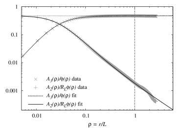
(a)

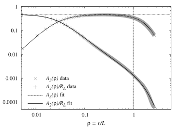
(b)

Figure 7: (a) The fit for $A_{2}(\rho)/R_{L}\phi(\rho)$, as given by equation (27), to present DNS data. This also determines $A_{3}(\rho)/\phi(\rho)$; see equation (26). The fit was performed for the region $\rho\leq 1$. (b) The equivalent fit for $A_{3}(\rho)$ and $A_{2}(\rho)/R_{L}$. In both parts, $C_{\varepsilon}$ is indicated by the horizontal dotted line.

The expression for $A_{2}(\rho)/R_{L}\phi(\rho)$ given by equation (27) was fitted to the present DNS data to find $a,\ b$ and $\gamma$. This also fixed the form for $A_{3}(\rho)/\phi(\rho)$, as given by equation (26). The fit was performed up to the integral scale, $\rho=1$, as shown in Fig. 7(a) by the vertical dash-dot line, above which the simulations become less well resolved. Clearly, agreement is excellent for $\rho<1$. Figure 7(b) then uses the measured function $\phi(\rho)$ to plot the equivalent fit to DNS data for $A_{3}$ and $A_{2}/R_{L}$. The scale dependence of $A_{2}$ and $A_{3}$ is, therefore, well modelled by our choice of profile function, $H(\rho)$. As a consequence, the scale dependence in equation (25) cancels out in such a way that $C_{\varepsilon}(R_{L})$ can still be modelled using equation (21), despite finite forcing introducing scale dependence $\phi(\rho)$ to the input term. One could therefore replace $C_{\varepsilon}$ in equations (26) and (27) with $\big{[}C_{\varepsilon,\infty}+C_{L}/R_{L}\big{]}$.

V Conclusions

We have presented a new form of the KHE for forced turbulence which differs from that commonly found in the literature. In deriving this equation from the Lin equation, we have obtained a scale-dependent energy input term (7). Our new form of the general KHE, equation (5), correctly reduces to the well-known form for decaying turbulence.

By scaling the forced KHE into a dimensionless form (17), we see that the appropriate Reynolds number for studying the variation of the dimensionless dissipation, $C_{\varepsilon}$, is that corresponding to the integral scale, $R_{L}$. In the limit of $\delta(\boldsymbol{\mathbf{k}})$-forcing, or for scales well below the influence of any forcing, the dimensionless equation suggests the simple model (21) for the balance of inertial and viscous contributions to the dimensionless dissipation rate. The new model has been fitted to the present DNS data with excellent agreement. It also shows that the behaviour of the dimensionless dissipation rate, as found experimentally, is entirely in accord with the Kolmogorov (K41) picture of turbulence and, in particular, with Kolmogorov’s derivation of his ‘$4/5$’ law Kolmogorov (1941), the one universally accepted result in turbulence.

The scale dependence of the inertial and viscous terms, $A_{3}$ and $A_{2}$, caused by finite forcing have been shown to compensate one another exactly (25), and as such have been modelled by a single profile function $H(\rho)$. The scale independence of equation (25) can then be used to motivate the application of the model given by equation (21) to general, finite forcing.

The authors thank Matthew Salewski for reading the manuscript and making a number of helpful comments. AB and SY were funded by the STFC. We thank one of the referees for drawing our attention to the statistically significant lack of energy conservation in simulations with $R_{\lambda}<25$ and also for pointing out the implications of the small-scale limit for the ad hoc profile function.

References

- Taylor (1935) G. I. Taylor, Proc. R. Soc., London, Ser. A 151, 421 (1935).
- Batchelor (1971) G. K. Batchelor, The theory of homogeneous turbulence (Cambridge University Press, Cambridge, 1971), 2nd ed.
- Sreenivasan (1984) K. R. Sreenivasan, Phys. Fluids 27, 1048 (1984).
- Sreenivasan (1998) K. R. Sreenivasan, Phys. Fluids 10, 528 (1998).
- Saffman (1968) P. G. Saffman, in Topics in nonlinear physics, edited by N. Zabusky (Springer-Verlag, 1968), pp. 485–614.
- Lohse (1994) D. Lohse, Phys. Rev. Lett. 73, 3223 (1994).
- Doering and Foias (2002) C. R. Doering and C. Foias, J. Fluid Mech. 467, 289 (2002).
- McComb et al. (2010) W. D. McComb, A. Berera, M. Salewski, and S. R. Yoffe, Phys. Fluids 22, 61704 (2010).
- Jiménez et al. (1993) J. Jiménez, A. A. Wray, P. G. Saffman, and R. S. Rogallo, J. Fluid Mech. 255, 65 (1993).
- Yamazaki et al. (2002) Y. Yamazaki, T. Ishihara, and Y. Kaneda, J. Phys. Soc. Jap. 71, 777 (2002).
- Kaneda et al. (2003) Y. Kaneda, T. Ishihara, M. Yokokawa, K. Itakura, and A. Uno, Phys. Fluids 15, L21 (2003).
- Kaneda and Ishihara (2006) Y. Kaneda and T. Ishihara, Journal of Turbulence 7, 1 (2006).
- Doering and Petrov (2005) C. R. Doering and N. P. Petrov, Progress in Turbulence 101, 11 (2005).
- Taylor and Green (1937) G. I. Taylor and A. Green, Proc. Roy. Soc. London A 158, 499 (1937).
- Brachet et al. (1983) M. E. Brachet, D. I. Meiron, S. A. Orszag, B. G. Nickel, R. H. Morf, and U. Frisch, J. Fluid Mech. 130, 411 (1983).
- Wang et al. (1996) L.-P. Wang, S. Chen, J. G. Brasseur, and J. C. Wyngaard, J. Fluid Mech. 309, 113 (1996).
- Cao et al. (1999) N. Cao, S. Chen, and G. D. Doolen, Phys. Fluids 11, 2235 (1999).
- Gotoh et al. (2002) T. Gotoh, D. Fukayama, and T. Nakano, Phys. Fluids 14, 1065 (2002).
- Donzis et al. (2005) D. A. Donzis, K. R. Sreenivasan, and P. K. Yeung, J. Fluid Mech. 532, 199 (2005).
- Bos et al. (2007) W. J. T. Bos, L. Shao, and J.-P. Bertoglio, Phys. Fluids 19, 45101 (2007).
- McComb (1990) W. D. McComb, The Physics of Fluid Turbulence (Oxford University Press, 1990).
- Monin and Yaglom (1975) A. S. Monin and A. M. Yaglom, Statistical Fluid Mechanics (MIT Press, 1975).
- Sirovich et al. (1994) L. Sirovich, L. Smith, and V. Yakhot, Phys. Rev. Lett. 72, 344 (1994).
- Kolmogorov (1941) A. N. Kolmogorov, C. R. Acad. Sci. URSS 32, 16 (1941).
- Batchelor (1953) G. K. Batchelor, The theory of homogeneous turbulence (Cambridge University Press, Cambridge, 1953), 1st ed.
- Qian (1997) J. Qian, Physical Review E 55, 337 (1997).
- Qian (1999) J. Qian, Physical Review E 60, 3409 (1999).
- Tchoufag et al. (2012) J. Tchoufag, P. Sagaut, and C. Cambon, Phys. Fluids 24, 015107 (2012).
- Pearson et al. (2002) B. R. Pearson, P. A. Krogstad, and de Water W. van, Phys. Fluids 14, 1288 (2002).