The core shift effect in the blazar 3C 454.3

Abstract

Opacity-driven shifts of the apparent VLBI core position with frequency (the “core shift” effect) probe physical conditions in the innermost parts of jets in active galactic nuclei. We present the first detailed investigation of this effect in the brightest $\gamma$-ray blazar 3C 454.3 using direct measurements from simultaneous 4.6–43 GHz VLBA observations, and a time lag analysis of 4.8–37 GHz lightcurves from the UMRAO, CrAO, and Metsähovi observations in 2007–2009. The results support the standard Königl model of jet physics in the VLBI core region. The distance of the core from the jet origin $r_{\mathrm{c}}(\nu)$, the core size $W(\nu)$, and the lightcurve time lag $\Delta T(\nu)$ all depend on the observing frequency $\nu$ as $r_{\mathrm{c}}(\nu)\propto W(\nu)\propto\Delta T(\nu)\propto\nu^{-1/k}$. The obtained range of $k=0.6-0.8$ is consistent with the synchrotron self-absorption being the dominating opacity mechanism in the jet. The similar frequency dependence of $r_{\mathrm{c}}(\nu)$ and $W(\nu)$ suggests that the external pressure gradient does not dictate the jet geometry in the cm-band core region. Assuming equipartition, the magnetic field strength scales with distance $r$ as $B=0.4(r/1\,pc)^{-0.8}$ G. The total kinetic power of electron/positron jet is about $10^{44}$ ergs s^-1.

1 Introduction

3C 454.3, also known as PKS B2251$+$158 ($\alpha_{\mathrm{J2000}}$=22:53:57.747940 $\delta_{\mathrm{J2000}}$=$+$16:08:53.56074; $z=0.859$ Jackson & Browne 1991) and nicknamed the “Crazy Diamond” by the AGILE team for its brightness and unpredictable behavior (Vercellone et al. 2010), is a prominent member of the blazar class of active galactic nuclei. Like other blazars, 3C 454.3 contains a relativistic plasma jet pointed close to our line of sight. As a result of relativistic beaming, synchrotron radiation from the jet dominates the blazar’s observed energy output from radio to infrared and optical bands (Marscher 1980). During a low flux density state, when the jet emission is weak, a prominent ultraviolet excess is observed which is attributed to thermal emission of the accretion disk (e.g., Smith et al. 1988, Villata et al. 2009, Raiteri et al. 2011). The bright X-ray to GeV emission of 3C 454.3 is likely due to inverse Compton scattering of photons from an external source (a broad-line region gas, accretion disk or dusty torus) by relativistic leptons in the jet (e.g., Dermer et al. 2009). In 2008–2010 3C 454.3 showed a spectacular series of GeV flares becoming the brightest object in the $\gamma$-ray sky (Abdo et al. 2009, Striani et al. 2010, Ackermann et al. 2010, Bonnoli et al. 2011, Abdo et al. 2011, Vercellone et al. 2011). The $\gamma$-ray flares were echoed in other bands (Villata et al. 2009, Sakamoto et al. 2009, Vercellone et al. 2010, Jorstad et al. 2010, Pacciani et al. 2010), but the corresponding optical flares were not exceptional for this blazar (Krajci et al. 2010). So far, the object was not detected in TeV band (Anderhub et al. 2009).

Radio observations with the Very Long Baseline Interferometry (VLBI) technique provide images of extragalactic jets with spatial resolution of an order of a parsec (e.g., Pearson 1996, Zensus 1997, Zensus et al. 2006, Lobanov 2010). The structure of most blazars, including 3C 454.3 (Fig. 1), is dominated by a bright, unresolved or barely-resolved feature called the core. The core has a flat or inverted radio spectrum, characteristic of optically-thick synchrotron emission (e.g., Kaiser 2006, Potter & Cotter 2012). shorter than any other jet structure. Evidence is growing that processes close to the VLBI core are responsible for the high-energy emission of blazars (e.g., Kovalev et al. 2009, Pushkarev et al. 2010, León-Tavares et al. 2011, Schinzel et al. 2012, Wehrle et al. 2012). The physical nature of the parsec-scale core is still being debated (Marscher 2006, 2008), however the most widely accepted interpretation is that the core is a surface in a continuous flow where the optical depth of jet’s synchrotron radiation $\tau_{\nu}\approx 1$ – “photosphere” (Readhead et al. 1979, Konigl 1981, Zensus et al. 1995).

The standard jet model (Blandford & Königl 1979, Konigl 1981) predicts that the apparent position of the photosphere (and, therefore, the VLBI core if the above interpretation is correct) depends on the observing frequency. This is known as the “core shift” effect and it was first observed by Marcaide & Shapiro (1984) in the quasar pair 1038$+$528 A, B and later in other sources by, among others, Zensus et al. (1995), Lobanov (1998), Paragi et al. (2000), Kovalev et al. (2008), O’Sullivan & Gabuzda (2009), Sokolovsky et al. (2011a), Hada et al. (2011), Algaba et al. (2012), and Pushkarev et al. (2012). Measurements of the frequency-dependent core position shift may provide important information about the physical conditions and structure of ultra compact blazar jets (Lobanov 1998, Hirotani 2005, O’Sullivan & Gabuzda 2009). Such observations may constrain the nature of the absorbing material: synchrotron self-absorption (SSA) within the jet plasma vs. free-free absorption in thermal plasma surrounding the jet. While SSA appears to be the dominating opacity mechanism in blazar jets (Sokolovsky et al. 2011a), free–free absorption is found in relativistic jet sources viewed at large angles to the line of sight: Cyg A (Bach et al. 2008) and NGC 1052 (Kadler et al. 2004).

The core shift effect has important consequences for ultra-high precision astrometry (Rioja et al. 2005, Porcas 2009), radio (VLBI) to optical (GAIA) reference frame alignment (Kovalev et al. 2008) and spacecraft navigation with VLBI. It should be taken into account when constructing VLBI spectral index (e.g., Marr et al. 2001, Kovalev et al. 2008) and Faraday rotation maps (e.g., Hovatta et al. 2012).

This paper presents the first detailed study of the core shift effect in the quasar 3C 454.3 using both multi-frequency VLBI results and single-dish lightcurves. Core shift parameter estimates obtained independently from VLBA images and single-dish lightcurves are compared for the 2008 activity period of 3C 454.3. Methods to measure the core shift are discussed in Sect. 2, observational data are described in Sect. 3, Sect. 4 presents the employed analysis techniques, the results are discussed in Sect. 5. Throughout this work we assume the $\Lambda$CDM cosmology with the following parameters: $H_{0}=71$ km s^-1 Mpc^-1, $\Omega_{\mathrm{m}}=0.27$, and $\Omega_{\Lambda}=0.73$ (see Komatsu et al. 2009), which corresponds to a luminosity distance of $D_{L}=5489$ Mpc, an angular size distance of $D_{A}=1588$ Mpc, and a linear scale of 7.7 pc mas^-1 at the source redshift. We use positively defined spectral index $\alpha=d\ln S/d\ln\nu$.

2 Methods to measure the apparent core shift

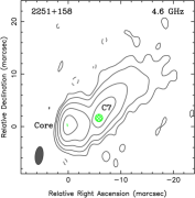
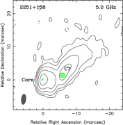
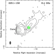
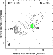
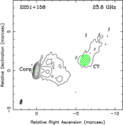
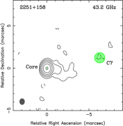
Figure 1: Naturally weighted total intensity CLEAN images of 3C 454.3. The image peaks are 3.3, 3.4, 6.3, 12.0, 15.8, 23.5 Jy/beam, for the 4.6, 5.0, 8.4, 15.4, 23.8, and 43.2 GHz frequencies, respectively. The contours starting at $6$ mJy/beam are plotted with a factor of 4 steps at all images. The beam is plotted in the lower left corner of each image at the half-power level. The 8.4 GHz image is almost identical to the 8.1 GHz one, which is not shown here. The observing epoch is 2 October 2008.

There is a number of ways to observe the core shift and related opacity-driven effects:

1. Direct apparent core position measurement through a phase-referencing experiment is the most obvious way to measure the core shift. In this method, the telescopes are switching between the target source and a nearby reference source (phase calibrator). The switching time is shorter than the coherence time, hence the calibrator’s phase solution can be applied to the target source. This allows one to preserve information about the target source position with respect to the phase calibrator. However, the method of measuring core shift using phase referencing has a few caveats. First, the reference source also experiences frequency-dependent position shift, sometimes even if the core is not the dominating feature of its structure (Sokolovsky et al. 2011b). Multiple reference sources could be used to overcome this problem (P. Voytsik et al., in prep.). Second, the technique is not free from ambiguities arising from modeling the source brightness distribution with a simplified model (typically, consisting of a few Gaussian emission components). This is true for the phase-referencing as well as for all the other VLBI-based core shift measurement techniques, because even if the absolute coordinate grid is established through the use of reference sources, the target source structure still has to be modeled to determine the position of its core. The phase-referencing method is also relatively expensive in terms of observing time.

2. The absolute position information is lost during the phase self-calibration procedure necessary for high-quality VLBI imaging. Therefore, it is not known a priori, how images at different frequencies should be aligned if phase-referencing is not applied. However, one may find a reference point in VLBI images that doesn’t change its position with frequency. In the absence of strong spectral index gradients, optically thin features in the jet may serve as such reference points. The core position may be measured with respect to an individual jet feature using a brightness distribution model (Kovalev et al. 2008, Sokolovsky et al. 2011a) or to a large jet section rich in structure by means of image cross-correlation (Croke & Gabuzda 2008, O’Sullivan & Gabuzda 2009, Algaba et al. 2012, Hovatta et al. 2012, Pushkarev et al. 2012). Both methods provide comparable results as was shown by Pushkarev et al. (2012).

3. The opacity effect also manifests itself as the core size increase at lower observing frequencies. For a conical jet, its cross-section size depends linearly on the distance from the cone apex (e.g., Fromm et al. 2011). In this case, the core size as a function of frequency should obey a power law with the same index, $-1/k$, as the core position shift versus frequency (Blandford & Königl 1979, Konigl 1981, Unwin et al. 1994, Jiang et al. 1998, Yang et al. 2008). If the jet is not conical, the dependencies of core size and core position shift on frequency will differ (resulting in different values of $k$). The core size measurements are rarely used to study opacity because this region is often unresolved by ground-based VLBI.

4. Opacity is the reason for time delay of lower frequency radio emission peaks with respect to the ones at higher frequencies (e.g., Marscher & Gear 1985, Valtaoja et al. 1992, Fromm et al. 2011). Radio flares are believed to be caused by disturbances traveling down the jet. The radio flare peak at a given frequency occurs around the time the disturbance passes the core at this frequency. Therefore, a time delay between radio lightcurves at different frequencies may be directly related to the core shift parameters measured with VLBI (Bach et al. 2006, Kudryavtseva et al. 2011). The opacity shift inferred from the time lags can be reconciled with the core shift measurements from VLBI observations under the following assumptions. The first one is that a flare at a given frequency $\nu_{\mathrm{obs}}$ has its peak quite near the jet location, where we observe the core at this frequency (i.e. where the optical depth $\tau_{\nu_{\mathrm{obs}}}=1$). The second assumption is that the jet Doppler factor is constant, i.e. the plasma flow speed and the jet viewing angle are constant, so we can link measured distance to time. If the flow is accelerated, the relation between time lags and measured core positions will not be linear.

5. A new method allowing one to simultaneously measure the frequency dependent core position shift and its size change using the radio intraday variability (IDV) caused by interstellar scintillation was proposed by Macquart et al. (2013). The position offset between the scintillating component (presumably, the core) at different frequencies is causing a time delay between the IDV lightcurves at these frequencies. This delay is stable on timescales much longer that the scintillation timescale and thus can be distinguished from the refractive effects of interstellar medium. The angular scale of the scintillating source at a given frequency is estimated from the IDV variability timescale and parameters of the scattering screen.

3 Observational data

3.1 Single epoch VLBI data

3C 454.3 was observed on 2 October 2008 with National Radio Astronomy Observatory (NRAO) Very Long Baseline Array (VLBA) simultaneously at seven frequencies ($4.6$, $5.0$, $8.1$, $8.4$, $15.4$, $23.8$, and $43.2$ GHz) in the framework of our survey of parsec-scale radio spectra of twenty $\gamma$-ray bright blazars (Sokolovsky et al. 2010a, b, Sokolovsky 2011). The observation was conducted with 16 on-source scans (each 4-7 minutes long depending on frequency) spread over 9 hours.

The data reduction was conducted in the standard manner using the AIPS package (Greisen 1990). A special procedure, similar to the one described by Sokolovsky et al. (2011a), was applied to improve amplitude calibration of the correlated flux density resulting in $\sim 5$% calibration accuracy at $4.6$–$15.4$ GHz range and $\sim 10$% accuracy at $23.8$ and $43.2$ GHz. The Difmap software (Shepherd 1997) was used for imaging and modeling the $uv$-data. Details of the employed calibration and analysis technique were discussed by Sokolovsky (2011).

Fig. 1 shows total intensity VLBA images of 3C 454.3. While at $4.6$ GHz the source shows a bright extended jet, at $43.2$ GHz its structure is dominated by the bright compact core. The spectra of the core and the jet component C7 are presented in Fig. 2. C7 is the only component that could be identified across all observing bands (its detection at $43.2$ GHz required data tapering). This component has a steep radio spectrum and, consequently, it is considered to be optically thin. Therefore C7 may serve as a reference feature for multi-frequency image alignment. Actually, its spectrum slightly deviates from the power law at low frequencies and can be fit with the theoretical spectrum of a uniform synchrotron-emitting cloud. Since C7 is more extended than the core, its spectrum may be artificially softened due to the $uv$-coverage related flux density losses at high frequencies. This, however, does not change the conclusion that C7 is optically thin in the studied frequency range. The core spectrum is highly inverted with the spectral slope $\alpha_{\mathrm{core}}=+0.9$ compatible with a partially optically thick synchrotron emission of a non-uniform source.

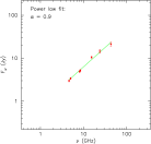
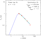
Figure 2: VLBA spectra of the core (left) and the reference jet component C7 (right) derived from $uv$-modeling. The observed spectra are compared to the power law (straight line in log-log scale) and uniform synchrotron cloud models.

3.2 Single-dish radio lightcurves from 4.8 to 37 GHz

Single-dish flux density monitoring observations of 3C 454.3 were obtained with the 26 m University of Michigan Radio Observatory (UMRAO) radio telescope at 4.8, 8.0 and 14.5 GHz, 14 m Metsähovi telescope at 22 and 37 GHz and the 22 m RT-22 radio telescope of Crimean Astrophysical Observatory (CrAO) at 22 and 37 GHz. The dataset and the corresponding observing techniques are presented and described by Vol’vach et al. (2011). The lightcurves of the 2008 flare are reproduced by us in Fig. 3. The flare duration is almost constant across all bands — slightly less than two years. One can see that the flare at lower frequencies is less prominent and delayed in time with respect to high frequencies with a time lag resulting from the synchrotron opacity (Shklovskii 1960, van der Laan 1966, Marscher & Gear 1985, Kudryavtseva et al. 2011) as discussed in Sect. 2 for the method 4.

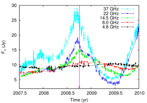
Figure 3: Radio lightcurves of the 2008 flare. The arrow marks the VLBA observation epoch.

4 Core shift analysis

We characterize the core shift effect using four different techniques of three methods as described in Sect. 2: VLBI core position shift measured with brightness distribution modeling and image cross-correlation (method 2), VLBI core size increase (method 3), and time-delay analysis of single-dish radio lightcurves (method 4).

4.1 Core position determined from modeling VLBA visibility data

Following Kovalev et al. (2008) and Sokolovsky et al. (2011a), we model jet emission at each frequency with a set of elliptical Gaussian components in the visibility ($uv$) plane. Fomalont (1999) formulas were applied to estimate position uncertainties of the model components. The well-isolated component C7 that could be identified across all the observing frequencies was chosen as the reference for determining the core position (Fig. 1). The distance, $\Delta r$, between the apparent core and C7 was measured at each frequency and fitted by $\Delta r=\frac{a}{\nu^{k}}+b$ law where $k=0.56\pm 0.22$ (Fig. 4, the best-fit values of coefficients $a$ and $b$ are presented in Table 1). The fact that C7 lies downstream of the region where the jet changes its direction from West to North-West should not affect the estimated value of $k$. Here and later the weighted non-linear least-square fitting is performed using the Levenberg–Marquardt algorithm (e.g, Press et al. 2002) and the reported parameter errors are the asymptotic standard errors obtained from the variance–covariance matrix after the final iteration.

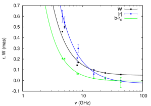
Figure 4: Measured values of the core shift ($|\vec{r}|$), core to C7 component separation ($r_{\mathrm{c}}$), and core width ($W$) as a function of $\nu$ compared to the corresponding $a\nu^{-1/k}+b$ fits (see Table 1).

4.2 Core position determined with 2D cross-correlation image analysis

3C 454.3 has a bright and extended parsec-scale jet rich in complex structures which make it well suited for image alignment with 2D cross-correlation. For each pair of adjacent frequencies in our observation we construct a pair of images convolved with the same beam (corresponding to the naturally weighted beam at the lower of the two frequencies). The pixel size is chosen as 1/20 of the minor axis of the restoring beam corresponding to the most optimistic positional accuracy expected for brightest image features. We have experimented with smaller pixel size but found no improvement in the image alignment accuracy.

A PDL-based program written by one of the authors (TS) was employed to perform the cross-correlation analysis. The same program was used by Hovatta et al. (2012) and Pushkarev et al. (2012). It allows a user to select an image region that contains complex structures expected to be optically thin above 5 GHz. We choose analysis regions containing most of the visible jet emission at each pair of images. The optically thick core region is excluded from the analysis. The process of manual region selection necessarily introduces a human bias in the process. In order to minimize this bias, we repeated each measurement multiple times selecting slightly different analysis regions. The obtained shifts were verified by visually examining the spectral index map constructed with the applied shift. The resulting map should not contain extreme spectral index values, especially near the edges of emitting regions (Marr et al. 2001, Kovalev et al. 2008, Hovatta et al. 2012). The difference in shifts obtained using different analysis regions, while the control spectral index map remained acceptable, were no greater than a few times 1/20 of the minor axis of the beam. We adopt this value as an indicator of the cross–correlation image alignment accuracy for a given frequency pair.

In order to test if the unmatched uv-coverage between the two frequencies has an impact on our results, for each pair of frequencies we repeated the analysis fixing the analyzed image areas and restricting the data to a common uv-range before convolving the images with the same beam. In all cases, the cross-correlation results differed by no more than one pixel from the ones obtained with the images having unmatched uv-coverage and convolved with the same beam. This confirms that restoring the two images with the same large beam effectively eliminates the effects of unmatched uv-coverage on cross-correlation analysis. We also correlated pairs of images restored with naturally-weighted beams after restricting the two data sets to the common uv-range. The two beams were not identical because, while the two data sets had the same uv-range, the uv-coverage within that range was slightly different. In that case, the cross-correlation results differed by up to 2 pixels from the ones obtained with images convolved with identical beams. Overall, the uncertainty of up to 2 pixels resulting from a choice of the analysis strategy (identical beams vs. different beams with matched uv-ranges) is no larger than the one introduced by a choice of an analyzed image area (a few pixels).

The cross–correlation method allows one to calculate a displacement, $\Delta\vec{r}_{12}$, between phase centers of images at two frequencies $\nu_{1}$ and $\nu_{2}$. When one knows $\Delta\vec{r}_{12}$, the core shift is calculated as $\Delta\vec{r}=\vec{r}_{1}+\Delta\vec{r}_{12}-\vec{r}_{2}$, where $\vec{r}_{1}$ and $\vec{r}_{2}$ are positions of the core relative to phase center at the two frequencies. Position of the core with respect to the phase center is measured by modeling the source structure in Difmap as in Sect. 4.1.

Pushkarev et al. (2012) reported the core shift of $0.159$ mas between 8 and 15 GHz measured with the VLBA for 3C 454.3 on 15 June 2006 using the same cross-correlation technique. This is close to the value obtained in our analysis (Table 1, Fig. 4).

It should be noted that for any given pair of frequencies, the value of core shift derived from the cross-correlation analysis, $|\vec{r}|$, is not the same as the difference in core separation from the jet component C7 derived from visibility model fitting (Sect. 4.1 and Table 1, column $r_{\mathrm{c}}$). The difference is clearly seen from comparing the $|\vec{r}|$ and $b$–$r_{\mathrm{c}}$ measurements and best-fit curves on Fig. 4. The reason is that the direction of $\vec{r}$ differs from the core – reference C7-component direction. However, if the angle between the two directions is constant, that will not affect estimation of the power-law coefficient $k$. The analysis using the cross-correlation method results in $k=0.68\pm 0.13$.

Table 1: Analysis results.

$\nu$	$|\vec{r}|$	$r_{\mathrm{c}}$	$W$	$\Delta T$
(GHz)	(mas)	(mas)	(mas)	(year)
43.2	$0.0$	$5.979\pm 0.046$	$0.055$	$\dots$
36.8	$\dots$	$\dots$	$\dots$	$0.0$
23.8	$0.02\pm 0.01$	$5.944\pm 0.013$	$0.071$	$\dots$
22.2	$\dots$	$\dots$	$\dots$	$0.04\pm 0.03$
15.4	$0.06\pm 0.04$	$5.936\pm 0.009$	$0.099$	$\dots$
14.5	$\dots$	$\dots$	$\dots$	$0.13\pm 0.03$
8.4	$0.30\pm 0.04$	$5.899\pm 0.007$	$0.169$	$\dots$
8.1	$0.21\pm 0.04$	$5.900\pm 0.008$	$0.143$	$\dots$
8.0	$\dots$	$\dots$	$\dots$	$0.39\pm 0.04$
5.0	$0.54\pm 0.06$	$5.756\pm 0.005$	$0.500$	$\dots$
4.8	$\dots$	$\dots$	$\dots$	$0.75\pm 0.07$
4.6	$0.60\pm 0.06$	$5.757\pm 0.004$	$0.456$	$\dots$
$a=$	$6.0\pm 2.6$	$-3.3\pm 3.0$	$4.6\pm 2.5$	$6.2\pm 1.4$
$b=$	$-0.03\pm 0.03$	$5.96\pm 0.04$	$0.05\pm 0.01$	$-0.06\pm 0.02$
$k=$	$0.68\pm 0.13$	$0.56\pm 0.22$	$0.60\pm 0.09$	$0.78\pm 0.08$

Column designation: Col. 1 – frequency, Col. 2 – core position shift from cross-correlation analysis, Col. 3 – core separation from the reference jet component C7, Col. 4 – core size on the half-power level, Col. 5 – lightcurve time delay with respect to the 36.8 GHz peak. The last three rows present the best values for coefficients in the $a\nu^{-1/k}+b$ fit to the data in the corresponding columns.

4.3 Core size as a function of frequency

We fitted the measured major axis of elliptical Gaussian core components versus frequency dependency with the function $W=a\nu^{-1/k}+b$ and obtained $k=0.60\pm 0.09$ (Table 1, Fig. 4), which is consistent with the values derived from the core position analysis above. The core size uncertainty estimated following Fomalont (1999) is unrealistically small at all frequencies due to the large core flux density. Therefore we do not report these error estimates in Table 1. Clearly, in this case, the error of the estimated core size is dominated by modeling uncertainties that are hard to quantify. At each frequency we check that the estimated core size is larger than the resolution limit computed following Lobanov (2005), Kovalev et al. (2005).

4.4 Time lag analysis of single-dish radio lightcurves

We analyze radio lightcurves of the 2008 flare (Fig. 3) to compare the results with our single-epoch multi-frequency VLBA observation obtained on 2 October 2008 around the time the flare peaks at 15 GHz. Following Peterson et al. (1998), we linearly interpolate the lightcurves to calculate the corresponding cross-correlation functions (CCF, Fig. 5). The comparison of this method with discrete CCF proposed by Edelson & Krolik (1988) results in a good agreement. The CCF is calculated between the lightcurves at 36.8 GHz and other frequencies. The time span of the flare is taken to be 2 years. For the 36.8 GHz lightcurve we set it to be 2007.5–2009.5. Time lags at low frequencies are non-negligible compared to the cross-correlation window width. Increasing the window width would cause the following 2009 flare, which rises at high frequencies, to be included in the analysis, which might affect results. Instead, we shift the two-year-wide analysis window for each frequency below 36.8 GHz. We compute CCF values for trial shifts in the range from 0 to 1 year. The shift that maximizes the CCF value is used to find the time lag between the lightcurves.

To estimate an error of the resulting time lag we used “FR-RSS” method described by Peterson et al. (1998) consisting of 1000 cycles of Monte Carlo flux density randomization together with modified bootstrapping, which allows us to account for estimated flux density measurement errors, errors due to data sampling and “outlier” points. We also add a normally-distributed random time shifts to the lightcurves within each simulation with a standard deviation equal to the mean separation between the observations. The cross-correlation peak distribution was obtained for 37 GHz with each frequency and the time lag error was estimated as the standard deviation of this distribution.

The time lags measured by us for the 2008 activity period (see Table 1) are in agreement with the values ($\Delta T_{\mathrm{37-22}}=0.03$ year and $\Delta T_{\mathrm{37-15}}=0.11$ year) obtained by Villata et al. (2007) for 2005–2007. See also Fig. 3 in Volvach et al. (2007). Pyatunina et al. (2007) report a wide range of time lags measured in 1990–2001 with typical values close to our results.

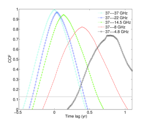
Figure 5: Cross-correlation function for the radio lightcurves.

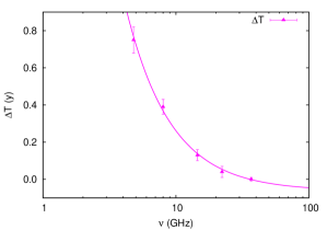
Figure 6: Measured values of the time lag, $\Delta T$, as a function of $\nu$ compared to the corresponding $a\nu^{-1/k}+b$ fit (see Table 1).

Fig. 6 illustrates the frequency dependence of the time delay with respect to the 37 GHz lightcurve. We perform a weighted nonlinear least-squares fit with the model $\Delta T=a\nu^{-1/k}+b$ which results in $k=0.78\pm 0.08$.

5 Discussion

The Konigl (1981) jet model assumes that magnetic field strength $B$ and particle density $N$ are declining with distance from the jet origin, $r$, according to the power law: $B=B_{1}(r/r_{1})^{-m}$, $N=N_{1}(r/r_{1})^{-n}$ (here $B_{1}$ and $N_{1}$ are values at $r=r_{1}=1$ pc from the jet base). The power law index $k$ in the relation of the core position, $r_{\mathrm{c}}$, and core size, $W$, change with frequency ($r_{\mathrm{c}}\propto W\propto\nu^{-1/k}$) depends on the magnetic field and particle density indexes $m$ and $n$ and the optically thin spectral index $\alpha$. If an equipartition fraction or jet power change along the jet, these changes will also affect the value of $k$ (Potter & Cotter 2013). To estimate $m$ and $n$ we consider two possible situations: 1) ambient medium pressure on the jet is negligible (Sec. 5.1) and 2) the external pressure is non-negligible and has a non-zero gradient along the jet (Sec. 5.3). For all calculations in this section we adopt $k=0.7\pm 0.1$.

5.1 Negligible ambient medium pressure

Assuming that the ambient medium pressure on the jet is negligible (the “free jet” assumption), we have

$$k=[(3-2\alpha)m+2n-2]/(5-2\alpha)$$ (1)

(Konigl 1981, Lobanov 1998), where $\alpha$ is the optically thin spectral index. The assumption of equipartition between the magnetic field and electron energy densities requires that

$$N_{1}(r/r_{1})^{-n}\gamma_{\mathrm{min}}m_{e}c^{2}=KB_{1}^{2}(r/r_{1})^{-2m}/8\pi,$$ (2)

therefore $n=2m$, where $m_{e}$ is the electron mass, $\gamma_{\mathrm{min}}$ is the minimal Lorentz-factor of emitting electrons, $K\approx 1/\ln(\gamma_{\mathrm{max}}/\gamma_{\mathrm{min}})\approx 0.1$ assuming optically thin spectral index $\alpha=-0.5$ and the maximum Lorentz-factor of emitting electrons $\gamma_{\mathrm{max}}=10^{4.34}\gamma_{\mathrm{min}}$ (Hirotani 2005).

If the jet flow speed is constant, the jet has a conical shape (constant opening angle) and the particle density $N\propto r^{-2}$ ($n=2$). In that case, the equipartition condition leads to $m=1$ and $k=1$ (for any $\alpha$). However, if jet flow speed and/or its opening angle are changing along the jet, other combinations of $m$, $n$, and $\alpha$ are possible that would satisfy the equipartition condition and result in $k\neq 1$. The values of $m$ and $n$ can be derived from (1) given the observed value of $k=0.7$ and assuming $\alpha=-0.5$: $m\simeq 0.8$, $n=2m=1.6$. We note that the result only weakly depends on the assumed value of $\alpha$.

The core position offset $\Delta r_{\mathrm{mas}}$ (expressed in milliarcseconds) between two frequencies $\nu_{1}$ and $\nu_{2}$ ($\nu_{1}<\nu_{2}$, GHz) may be expressed by the parameter (Lobanov 1998)

$$\Omega=4.85\cdot 10^{-9}\frac{\Delta r_{\mathrm{mas}}D_{\mathrm{L}}}{(1+z)^{2}}\left(\frac{\nu_{1}^{1/k}\nu_{2}^{1/k}}{\nu_{2}^{1/k}-\nu_{1}^{1/k}}\right),$$ (3)

where $D_{\mathrm{L}}$ is the luminosity distance in pc at the redshift $z$. Averaging over all the frequency pairs and excluding the close pairs 8.1/8.4 and 4.6/5.0 GHz we obtain $\Omega=43\pm 10$ pc GHz^1/k. Following O’Sullivan & Gabuzda (2009), we evaluate equation (43) from Hirotani (2005), assuming the equipartition condition (2), to estimate the magnetic field strength at 1 pc from the jet base:

$$B_{1}\approx 0.014\left(\frac{\Omega^{3k}(1+z)^{2}\ln{\gamma_{\mathrm{max}}/\gamma_{\mathrm{min}}}}{\delta^{2}\phi\sin^{3k-1}\theta}\right)^{1/4},$$ (4)

where $\theta$ is the jet viewing angle, $\phi$ is the jet half opening angle and $\delta\equiv[\Gamma(1-\beta\cos\theta)]^{-1}$ is the Doppler-factor.

Jorstad et al. (2010) measured a large variety of values of $\theta$, $\Gamma_{\mathrm{j}}$, and $\delta$ for three VLBI-components in 3C 454.3. They supposed that these components move along different sides of the jet (closer or farther from the line of sight). We adopt the average values measured by Jorstad et al. (2005): $\theta=1.3^{\circ}$, $\phi=0.8^{\circ}$, $\delta=24.6$, $\Gamma_{\mathrm{j}}=15.6$, the value of $k=0.7$ and $\ln(\gamma_{\mathrm{max}}/\gamma_{\mathrm{min}})=10$. Therefore we get $B_{1}=0.4\pm 0.2$ G. The estimated uncertainty is formally propagated from the adopted uncertainties of $k$ and $\Omega$. We note however, that the uncertainties of $\delta$, $\phi$, $\theta$ and $\ln(\gamma_{\mathrm{max}}/\gamma_{\mathrm{min}})$ also contribute to the total uncertainty. The obtained value of $B_{1}$ is close to the one estimated by Pushkarev et al. (2012) from 8–15 GHz core shift measurements with the assumption of $k=1$. Following Lobanov (1998) we estimate the core position at 43 GHz and, hence, the magnetic field in the 43 GHz core: $B_{\mathrm{43\,GHz~{}core}}=0.07\pm 0.04$ G. For the 15 GHz core: $B_{\mathrm{15\,GHz~{}core}}=0.02\pm 0.01$ G.

The de-projected distance of the core at a given frequency from the central engine may be estimated following Lobanov (1998), Hirotani (2005): $r_{\rm core}(\nu)=\frac{\Omega}{\sin\theta}\nu^{-1/k_{\rm r}}$. For the 43 GHz core, assuming the above value of $\theta$, $r_{\rm core}({\rm 43\,GHz})\sim 9$ pc. For the 15 GHz core, $r_{\rm core}({\rm 15\,GHz})\sim 38$ pc.

We can estimate the apparent jet half-opening angle by comparing core sizes and positions measured at different frequencies (Col. 4 and 2 in Table 1) as $\phi_{\mathrm{app}}\approx\Delta W/2\Delta r\approx 17^{\circ}$, which corresponds to the intrinsic half-opening angle $\phi=\phi_{\mathrm{app}}\sin\theta\approx 0.4^{\circ}$. This is two times smaller than the value used above. However our estimate is subject to uncertain modeling errors in W and we prefer to use the values of $\phi$ and $\theta$ obtained by Jorstad et al. (2005). If we use our value of $\phi$ instead, the magnetic field strength does not change within the estimated error.

5.2 Total jet power

The total jet power, often referred to as “kinetic luminosity”, can be computed within the equipartition assumption using equation (46) of Hirotani (2005). As input parameters for the computation we take the above values of $\theta$, $\phi$, $\delta$, and $\Gamma_{\mathrm{j}}$ determined by Jorstad et al. (2005), the measured values $k=0.7$, $\alpha=-0.5$ and assume constant $\Gamma_{\mathrm{j}}$ along the jet. The two critical assumptions are the minimum Lorentz factor of the emitting particles, $\gamma_{\mathrm{min}}=100$ (Hirotani 2005), and jet composition (electron/positron vs. electron/proton plasma). For an electron/positron jet, the total kinetic power is a few $\times 10^{44}$ ergs s^-1. For the same $\gamma_{\mathrm{min}}$, the electron/proton jet would be $m_{p+}/m_{e-}=1836.2$ times more powerful.

5.3 External pressure gradient

If the external pressure drops along the jet as $p\propto r^{-a}$, the jet will be constantly accelerating as $\Gamma_{\mathrm{j}}=\Gamma_{\mathrm{j\ast}}(r/r_{\ast})^{a/4}$, where $r$ is axial jet coordinate and values marked with $\ast$ are related to the point where jet becomes supersonic (Georganopoulos & Marscher 1996). For $r\gg r_{\ast}$ the jet cross-section $d\propto r^{a/4}$ (the observed core size $W\approx d$). The depicted situation is true in a hydrodynamically accelerating and adiabatic, steady-state jet. In this case, the core size dependence on the observing frequency ($W(\nu)\propto\nu^{-a/(4k)}$) differs from the one of the core position offset ($r\propto\nu^{-1/k}$) if $a\neq 4$.

The measured value of $k$ may be related to the pressure gradient $a$ (see Fig. 1 in Lobanov 1998) resulting in $a\simeq 2.2$. Hence the magnetic field and particle density power-law indexes become $m_{p}\approx 0.4$ and $n_{p}\approx 2.2$. However, the power law coefficients for $W(\nu)$ and $r(\nu)$ would differ by a factor of $a/4\simeq 0.55$ which contradicts the obtained values (Table 1). We conclude that the external pressure gradient is not a dominant factor in determining the jet geometry in the region of 43–4.6 GHz core of 3C 454.3.

5.4 Jet speed estimated from time lags and core shift

Assuming that a lightcurve peak at a given frequency, $\nu$, occurs when a plasma condensation (jet component) traveling down the jet passes the region of the core at that frequency, $r_{\nu}$, one can estimate the apparent projected speed of such a plasma condensation by comparing the lightcurve time delay, $\Delta T$, with the VLBI core position shift between a pair of frequencies, $\Delta r$: $\mu_{\mathrm{app}}=\Delta r/\Delta T\simeq 0.7$ mas/yr (the exact value depends on the choice of the frequency pair). This value is 2–8 times larger than $\mu_{\mathrm{app}}$ directly measured with VLBI by Lister et al. (2009) and Jorstad et al. (2010). One possible explanation for this discrepancy is that the 2008 flare might have been caused by an exceptionally fast jet component. This seems possible considering the wide distribution of individual component’s velocities observed with VLBI. On the other hand, the discrepancy may result from the limited applicability of the above assumption. If the peak flux density of the flaring component is declining while the flare develops and the component becomes optically thin at progressively lower frequencies (as expected for the adiabatic losses dominated stage of flare development, Marscher & Gear 1985), the lightcurve peak would occur earlier than the component reaches the position in the jet marked by the quiescent core at this frequency. This will result in an overestimated component velocity since the time lag between peaks will be smaller than the time it takes for the component to travel between the higher- and lower-frequency core positions. In principle, one could also suggest that VLBI does not always measure the apparent speed which represents the true plasma flow speed. A hint that this might be the case comes from comparing results of VLBA kinematics measurements in the inner jet of M87 at 2 cm (Kovalev et al. 2007) and 7 mm (Ly et al. 2007).

6 Summary

In the jet model of Blandford & Königl (1979) and Konigl (1981), synchrotron opacity manifests itself in the frequency-dependent position and size of the apparent VLBI core, as well as in the time delay between radio lightcurves obtained at different frequencies. We observe these effects in 3C 454.3 using 4.6–43 GHz VLBA images and 4.8–37 GHz lightcurves obtained with the 26 m UMRAO, 22 m CrAO, and 14 m Metsähovi telescopes in 2007–2009.

Our results support this model as an appropriate description of jet physics in the apparent parsec-scale core region. The distance of the core from the jet origin $r_{\mathrm{c}}(\nu)$, the core size $W(\nu)$, and the lightcurve time lag $\Delta T(\nu)$ all depend on the observing frequency $\nu$ as $r_{\mathrm{c}}(\nu)\propto W(\nu)\propto\Delta T(\nu)\propto\nu^{-1/k}$. We find the value of the coefficient to be in the range $k=$ 0.6–0.8, consistent with the synchrotron self-absorption being the dominating opacity mechanism in the jet of 3C 454.3, as opposed to free-free absorption found in relativistic jet sources viewed at large angles to the line of sight, e.g., Cyg A (Bach et al. 2008) and NGC 1052 (Kadler et al. 2004). Zamaninasab et al. (2013 A&A submitted) analyzed two epochs (2005-05-19 and 2009-09-22) of simultaneous multi-frequency (5–86 GHz) VLBA observations of 3C 454.3 and obtained the values of $k=0.9\pm 0.2$ and $k=0.8\pm 0.3$ for the 2005 and 2009 epochs, respectively. No difference between the frequency dependence of $r_{\mathrm{c}}(\nu)$ and $W(\nu)$ is observed which suggests that the external pressure is not significant for the jet geometry in the cm-band core region of 3C 454.3.

Assuming equipartition, we estimate the magnetic field strength 1 pc from the jet origin to be $B_{1}\sim 0.4$ G. It scales with distance from the central engine as $B=0.4(r/r_{1})^{-0.8}$ G. Within the equipartition assumption, the total kinetic power of the jet, assuming electron/positron composition and $\gamma_{\mathrm{min}}=100$, is a few $\times 10^{44}$ ergs s^-1. The electron/proton jet would be about two thousand times more powerful.

The remarkable agreement found between results obtained with different techniques both improves robustness of presented results and supports the lightcurve time lag measurements as an efficient tool to study characteristics of the opaque apparent base of AGN jets.

References

- Abdo et al. (2011) Abdo A. A. et al., 2011, ApJ, 733, L26
- Abdo et al. (2009) Abdo A. A. et al., 2009, ApJ, 699, 817
- Ackermann et al. (2010) Ackermann M. et al., 2010, ApJ, 721, 1383
- Algaba et al. (2012) Algaba J. C., Gabuzda D. C., Smith P. S., 2012, MNRAS, 420, 542
- Anderhub et al. (2009) Anderhub H. et al., 2009, A&A, 498, 83
- Bach et al. (2008) Bach U., Krichbaum T. P., Middelberg E., Alef W., Zensus A. J., 2008, in The role of VLBI in the Golden Age for Radio Astronomy
- Bach et al. (2006) Bach U. et al., 2006, A&A, 456, 105
- Blandford & Königl (1979) Blandford R. D., Königl A., 1979, ApJ, 232, 34
- Bonnoli et al. (2011) Bonnoli G., Ghisellini G., Foschini L., Tavecchio F., Ghirlanda G., 2011, MNRAS, 410, 368
- Croke & Gabuzda (2008) Croke S. M., Gabuzda D. C., 2008, MNRAS, 386, 619
- Dermer et al. (2009) Dermer C. D., Finke J. D., Krug H., Böttcher M., 2009, ApJ, 692, 32
- Edelson & Krolik (1988) Edelson R. A., Krolik J. H., 1988, ApJ, 333, 646
- Fomalont (1999) Fomalont E. B., 1999, in Astronomical Society of the Pacific Conference Series, Vol. 180, Synthesis Imaging in Radio Astronomy II, Taylor G. B., Carilli C. L., Perley R. A., eds., p. 301
- Fromm et al. (2011) Fromm C. M. et al., 2011, A&A, 531, A95
- Georganopoulos & Marscher (1996) Georganopoulos M., Marscher A. P., 1996, in Astronomical Society of the Pacific Conference Series, Vol. 110, Blazar Continuum Variability, Miller H. R., Webb J. R., Noble J. C., eds., p. 262
- Greisen (1990) Greisen E. W., 1990, in Acquisition, Processing and Archiving of Astronomical Images, G. Longo & G. Sedmak, ed., pp. 125–142
- Hada et al. (2011) Hada K., Doi A., Kino M., Nagai H., Hagiwara Y., Kawaguchi N., 2011, Nature, 477, 185
- Hirotani (2005) Hirotani K., 2005, ApJ, 619, 73
- Hovatta et al. (2012) Hovatta T., Lister M. L., Aller M. F., Aller H. D., Homan D. C., Kovalev Y. Y., Pushkarev A. B., Savolainen T., 2012, AJ, 144, 105
- Jackson & Browne (1991) Jackson N., Browne I. W. A., 1991, MNRAS, 250, 414
- Jiang et al. (1998) Jiang D. R., Cao X., Hong X., 1998, ApJ, 494, 139
- Jorstad et al. (2010) Jorstad S. G. et al., 2010, ApJ, 715, 362
- Jorstad et al. (2005) Jorstad S. G. et al., 2005, AJ, 130, 1418
- Kadler et al. (2004) Kadler M., Ros E., Lobanov A. P., Falcke H., Zensus J. A., 2004, A&A, 426, 481
- Kaiser (2006) Kaiser C. R., 2006, MNRAS, 367, 1083
- Komatsu et al. (2009) Komatsu E. et al., 2009, ApJS, 180, 330
- Konigl (1981) Konigl A., 1981, ApJ, 243, 700
- Kovalev et al. (2009) Kovalev Y. Y. et al., 2009, ApJ, 696, L17
- Kovalev et al. (2005) Kovalev Y. Y. et al., 2005, AJ, 130, 2473
- Kovalev et al. (2007) Kovalev Y. Y., Lister M. L., Homan D. C., Kellermann K. I., 2007, ApJ, 668, L27
- Kovalev et al. (2008) Kovalev Y. Y., Lobanov A. P., Pushkarev A. B., Zensus J. A., 2008, A&A, 483, 759
- Krajci et al. (2010) Krajci T., Sokolovsky K., Henden A., 2010, The Astronomer’s Telegram, 3047, 1
- Kudryavtseva et al. (2011) Kudryavtseva N. A., Gabuzda D. C., Aller M. F., Aller H. D., 2011, MNRAS, 415, 1631
- León-Tavares et al. (2011) León-Tavares J., Valtaoja E., Tornikoski M., Lähteenmäki A., Nieppola E., 2011, A&A, 532, A146
- Lister et al. (2009) Lister M. L. et al., 2009, AJ, 138, 1874
- Lobanov (1998) Lobanov A. P., 1998, A&A, 330, 79
- Lobanov (2005) Lobanov A. P., 2005, ArXiv:astro-ph/0503225
- Lobanov (2010) Lobanov A. P., 2010, ArXiv:1010.2856
- Ly et al. (2007) Ly C., Walker R. C., Junor W., 2007, ApJ, 660, 200
- Macquart et al. (2013) Macquart J.-P., Godfrey L. E. H., Bignall H. E., Hodgson J. A., 2013, ApJ, 765, 142
- Marcaide & Shapiro (1984) Marcaide J. M., Shapiro I. I., 1984, ApJ, 276, 56
- Marr et al. (2001) Marr J. M., Taylor G. B., Crawford, III F., 2001, ApJ, 550, 160
- Marscher (1980) Marscher A. P., 1980, ApJ, 235, 386
- Marscher (2006) Marscher A. P., 2006, in American Institute of Physics Conference Series, Vol. 856, Relativistic Jets: The Common Physics of AGN, Microquasars, and Gamma-Ray Bursts, P. A. Hughes & J. N. Bregman, ed., pp. 1–22
- Marscher (2008) Marscher A. P., 2008, in Astronomical Society of the Pacific Conference Series, Vol. 386, Extragalactic Jets: Theory and Observation from Radio to Gamma Ray, T. A. Rector & D. S. De Young, ed., p. 437
- Marscher & Gear (1985) Marscher A. P., Gear W. K., 1985, ApJ, 298, 114
- O’Sullivan & Gabuzda (2009) O’Sullivan S. P., Gabuzda D. C., 2009, MNRAS, 400, 26
- Pacciani et al. (2010) Pacciani L. et al., 2010, ApJ, 716, L170
- Paragi et al. (2000) Paragi Z., Fejes I., Frey S., 2000, in International VLBI Service for Geodesy and Astrometry 2000 General Meeting Proceedings, N. R. Vandenberg & K. D. Baver, ed., p. 342
- Pearson (1996) Pearson T. J., 1996, in Astronomical Society of the Pacific Conference Series, Vol. 100, Energy Transport in Radio Galaxies and Quasars, P. E. Hardee, A. H. Bridle, & J. A. Zensus, ed., p. 97
- Peterson et al. (1998) Peterson B. M., Wanders I., Horne K., Collier S., Alexander T., Kaspi S., Maoz D., 1998, PASP, 110, 660
- Porcas (2009) Porcas R. W., 2009, A&A, 505, L1
- Potter & Cotter (2012) Potter W. J., Cotter G., 2012, MNRAS, 423, 756
- Potter & Cotter (2013) Potter W. J., Cotter G., 2013, MNRAS, 431, 1840
- Press et al. (2002) Press W. H., Teukolsky S. A., Vetterling W. T., Flannery B. P., 2002, Numerical recipes in C++ : the art of scientific computing
- Pushkarev et al. (2012) Pushkarev A. B., Hovatta T., Kovalev Y. Y., Lister M. L., Lobanov A. P., Savolainen T., Zensus J. A., 2012, A&A, 545, A113
- Pushkarev et al. (2010) Pushkarev A. B., Kovalev Y. Y., Lister M. L., 2010, ApJ, 722, L7
- Pyatunina et al. (2007) Pyatunina T. B., Kudryavtseva N. A., Gabuzda D. C., Jorstad S. G., Aller M. F., Aller H. D., Teräsranta H., 2007, MNRAS, 381, 797
- Raiteri et al. (2011) Raiteri C. M. et al., 2011, A&A, 534, A87
- Readhead et al. (1979) Readhead A. C. S., Pearson T. J., Cohen M. H., Ewing M. S., Moffet A. T., 1979, ApJ, 231, 299
- Rioja et al. (2005) Rioja M. J., Dodson R., Porcas R. W., Suda H., Colomer F., 2005, ArXiv:astro-ph/0505475
- Sakamoto et al. (2009) Sakamoto T., D’Ammando F., Gehrels N., Kovalev Y. Y., Sokolovsky K., 2009, The Astronomer’s Telegram, 2329, 1
- Schinzel et al. (2012) Schinzel F. K., Lobanov A. P., Taylor G. B., Jorstad S. G., Marscher A. P., Zensus J. A., 2012, A&A, 537, A70
- Shepherd (1997) Shepherd M. C., 1997, in Astronomical Society of the Pacific Conference Series, Vol. 125, Astronomical Data Analysis Software and Systems VI, G. Hunt & H. Payne, ed., p. 77
- Shklovskii (1960) Shklovskii I. S., 1960, Soviet Ast., 4, 243
- Smith et al. (1988) Smith P. S., Elston R., Berriman G., Allen R. G., Balonek T. J., 1988, ApJ, 326, L39
- Sokolovsky (2011) Sokolovsky K., 2011, PhD thesis, Max-Planck-Institut für Radioastronomie
- Sokolovsky et al. (2010a) Sokolovsky K. V. et al., 2010a, ArXiv:1006.3084
- Sokolovsky et al. (2010b) Sokolovsky K. V., Kovalev Y. Y., Lobanov A. P., Savolainen T., Pushkarev A. B., Kadler M., 2010b, ArXiv:1001.2591
- Sokolovsky et al. (2011a) Sokolovsky K. V., Kovalev Y. Y., Pushkarev A. B., Lobanov A. P., 2011a, A&A, 532, A38
- Sokolovsky et al. (2011b) Sokolovsky K. V., Kovalev Y. Y., Pushkarev A. B., Mimica P., Perucho M., 2011b, A&A, 535, A24
- Striani et al. (2010) Striani E. et al., 2010, ApJ, 718, 455
- Unwin et al. (1994) Unwin S. C., Wehrle A. E., Urry C. M., Gilmore D. M., Barton E. J., Kjerulf B. C., Zensus J. A., Rabaca C. R., 1994, ApJ, 432, 103
- Valtaoja et al. (1992) Valtaoja E., Terasranta H., Urpo S., Nesterov N. S., Lainela M., Valtonen M., 1992, A&A, 254, 71
- van der Laan (1966) van der Laan H., 1966, Nature, 211, 1131
- Vercellone et al. (2010) Vercellone S. et al., 2010, ApJ, 712, 405
- Vercellone et al. (2011) Vercellone S. et al., 2011, ApJ, 736, L38
- Villata et al. (2007) Villata M. et al., 2007, A&A, 464, L5
- Villata et al. (2009) Villata M. et al., 2009, A&A, 504, L9
- Vol’vach et al. (2011) Vol’vach A. E. et al., 2011, Astronomy Reports, 55, 608
- Volvach et al. (2007) Volvach A. E., Volvach L. N., Larionov M. G., Aller H. D., Aller M. F., 2007, Astronomy Reports, 51, 450
- Wehrle et al. (2012) Wehrle A. E. et al., 2012, ApJ, 758, 72
- Yang et al. (2008) Yang J., Gurvits L. I., Frey S., Lobanov A. P., 2008, ArXiv:0811.2926
- Zensus (1997) Zensus J. A., 1997, ARA&A, 35, 607
- Zensus et al. (1995) Zensus J. A., Cohen M. H., Unwin S. C., 1995, ApJ, 443, 35
- Zensus et al. (2006) Zensus J. A., Krichbaum T. P., Britzen S., 2006, ArXiv:astro-ph/0610712